
Study on Urban Rainfall–Runoff Model under the Background of Inter-Basin Water Transfer

1
College of Urban and Environmental Sciences, Peking University, No. 5 Yiheyuan Road, Haidian District, Beijing 100871, China
2
School of Architecture, Tsinghua University, No. 30 Shuangqing Road, Haidian District, Beijing 100084, China
3
China Academy of Building Research, Beijing 100013, China
*
Author to whom correspondence should be addressed.
Water 2022, 14(17), 2660; https://doi.org/10.3390/w14172660
Submission received: 5 July 2022
/
Revised: 25 August 2022
/
Accepted: 25 August 2022
/
Published: 28 August 2022
(This article belongs to the Special Issue Advanced Hydrologic Modeling in Watershed Scales)
Abstract
:The imbalance of water supply and demand forces many cities to transfer water across basins, which changes the original “rainfall–runoff” relationship in urban basins. Long-term hydrological simulation of urban basins requires a tool that comprehensively considers the relationship of “rainfall–runoff” and the background of inter-basin water transfer. This paper combines the rainfall–runoff model, the GR3 model, with the background of inter-basin water transfer to simulate the hydrological process of Huangtaiqiao basin (321 km2) in Jinan city, Shandong Province, China for 18 consecutive years with a 1 h time step. Twenty-one flood simulation results of different scales over 18 years were selected for statistical analysis. By comparing the simulation results of the GR3 model and the measured process, the results were verified by multiple evaluation indicators (the Nash–Sutcliffe efficiency coefficient, water relative error, the relative error of flood peak flow, and difference of peak arrival time) at different time scales. It was found that the simulation results of the GR3 model after inter-basin water transfer were considered to be in good agreement with the measured data. This study proves the long-term impact of inter-basin water transfer on rainfall–runoff processes in an urban basin, and the GR3-ibwt model can better simulate the hydrological processes of urban basins, providing a new perspective and method.
1. Introduction
The distribution of global water resources is not balanced, and the demand for water in many regions far exceeds the amount of available water resources, leading to a break in the balance between the supply and demand of water resources [1,2,3,4]. This phenomenon is particularly obvious in China, where the uneven distribution of water resources in time and space makes the problem of water shortage in China’s regions increasingly serious [5,6,7]. Especially in urban areas, due to a large amount of industrial water, domestic water and other “urban water”, the amount of available water resources, which is not rich, becomes more scarce [8,9,10], forcing cities to exploit groundwater in large quantities [11,12,13,14], causing many problems [15,16,17]. In view of the above problems, inter-basin water transfer is an effective and direct method to solve the problems [18,19,20] and has been widely used in water-shortage areas around the world [21,22,23,24,25]. The South-to-North Water Diversion Project is a strategic project in China. Since it was fully completed in 2014, southern water has become the main source of water for more than 140 million people in more than 40 large and medium-sized cities such as Beijing and Tianjin [22,23,24,25].
As areas with a highly concentrated population, cities alleviate many problems, such as water resource shortages, through inter-basin water transfer projects on the one hand, while on the other hand, they are inevitably affected by other impacts brought by inter-basin water transfer [26], mainly manifested as changes in water quality [27] and river hydrological factors [26,28,29,30,31]. However, changes in hydrological elements such as river runoff and river water levels are related to urban flood control and drainage [32]. Urban floods occur frequently around the world and are highly harmful and destructive, affecting urban economic development and seriously threatening the life and property safety of urban residents [25,33,34]. Therefore, urban flood simulation has always been a research hotspot [35,36]. In the current context of inter-basin water transfer, many river basins are connected in series, and it has become a common phenomenon for cities to implement inter-basin water transfer [22]. Therefore, the impact of inter-basin water transfer on urban flood simulation has also become common. Essenfelder studied the flow contribution of inter-basin water transfer by incorporating machine learning techniques into basin hydrological models [23]. Woo et al. used a SWAT model to study the impact of inter-basin water transfer on water quality in the basin [24]. Bui et al. also used a SWAT model to study the impact of inter-basin water transfer on Lake Urmia in Iran and provided data support for the management of inter-basin water transfer [25]. However, few studies consider both the hydrological model and inter-basin water transfer, and only a few experts and scholars consider inter-basin water transfer using other tools. Safavi et al. used an artificial neural network (ANN) and a fuzzy inference system (FIS) to establish a model to simulate the river runoff of inter-basin water transfer cities [32]. Wang et al. used the MIKE series of hydrodynamic models to analyze the impact of inter-basin water transfer on flood control in water-receiving areas [33]. However, the water balance of urban basins is changed by inter-basin water transfer. The increased water volume of outer basins in urban basins means the water balance is no longer the same as in the relationship between rainfall, infiltration, evaporation, interception, and runoff in natural basins [37,38]. Although the rainfall–runoff model is an important tool for basin hydrological simulation [39,40], it is rarely used to study urban flood problems under the background of inter-basin water transfer, because inter-basin water transfer causes runoff and runoff in urban basins to no longer mirror the “rainfall–runoff” relationship in natural basins. As long as the problem of water balance in the basin is dealt with, the rainfall–runoff model is still the preferred choice for the hydrological simulation of a basin [41,42].
In this paper, the GR3 model, which has been proven to have good applicability in the Yangtze River basin, Yellow River basin, Heilongjiang River basin, Huaihe River basin, and other basins in China [43,44], is selected as the rainfall–runoff model for research. Xu et al. concluded that the simulation accuracy of the GR3 model and the Xinanjiang model, used in seven representative basins in China, is at the same level [44], while the Xinanjiang model has been widely used in China for decades [45,46,47]. At the same time, the distributed model requires a great deal of data and is very complex, but the simulation at the watershed outlet is not always better than the lumped (conceptual) model. Therefore, we chose the lumped (conceptual) GR3 model, which has fewer parameters, simple calibration, and can reduce the uncertainty of model parameters [48,49,50,51]. In order to study the impact of inter-basin water transfer on urban hydrological simulation, this paper chooses two scales, a long-time series and a single flood, to conduct hydrological simulation considering inter-basin water transfer and not considering inter-basin water transfer. This paper focuses on how to integrate the inter-basin water transfer into the GR3 model, using the GR3 model and the GR3 model combined with the inter-basin water transfer (hereinafter referred to as GR3-ibwt) to carry out multi-year (18 years) continuous hydrological simulations. Twenty-one flood simulation results of different scales over 18 years were selected for statistical analysis. Comparing the performance of the GR3 model and the GR3-ibwt model, we verified the simulation results on two scales of long-term series and single-flood processes, forming a new processing method. Section 2 outlines the materials and methods, Section 3 presents the results, Section 4 discusses these results, and Section 5 provides conclusions.
2. Materials and Methods
2.1. Study Area and Data Sources
In this study, the basin controlled by the Huangtaiqiao Hydrological Station in Jinan City (hereinafter referred to as the Huangtaiqiao basin) was selected as the study area. Jinan is also known as “Spring City”. There are many rivers and springs in the city, including The Yellow River, Xiaoqing River, Baotu Spring, Heihu Spring, and Pearl Spring, etc. [52], which are rich in water resources. Even so, Jinan still suffers from a severe water shortage. The average annual total water resources are 1.16 billion m3, and the per capita water resources are 210 m3, which is only 10% of China’s national standard and far lower than the global average of 1000 m³ [53,54]. The difference between the supply and demand of the available water resources is approximately 30% [54], which is a typical water-deficient city in northern China. The phenomenon of overexploitation of groundwater is serious, and the obstruction of spring water occurs from time to time [55]. Therefore, Jinan introduces approximately 600 million m³ of Yellow River water every year to supplement the water resource gap [56]. Since the completion of the eastern route of the South-to-North Water Diversion Project in 2013, Jinan has had to divert a large amount of water from the Yangtze River every year to supplement its water source [55]. A large number of water diversions from other basins have fully guaranteed the available water resources in Jinan, and groundwater exploitation has been effectively replaced [55,56]. However, the original water balance in the Huangtaiqiao basin was broken, and the runoff process of the Huangtaiqiao Hydrological Station was no longer a simple “rainfall–runoff” relationship. At the same time, Jinan is a city with frequent urban floods [57]. Due to the mountains in the south and the Yellow River in the north, the terrain is high in the south and low in the north, and the urban section of the Yellow River is an “above-ground river”. In addition, the annual precipitation is highly concentrated from June to September, which accounts for 70–80% of the annual precipitation. These factors cause frequent urban floods in Jinan [58]. On 18 July 2007, the “18 July” rainstorm in Jinan urban area had a maximum rainfall of 151 mm in one hour, which was the historical maximum since the meteorological records began in Jinan. The flood caused more than 30 deaths, more than 170 injuries, and direct economic losses of approximately 1.32 billion. RMB [59,60]. Jinan is not only a city with frequent floods [58], but also utilizes a large number of inter-basin water transfers [55,56]. Therefore, the Huangtaiqiao basin was selected as the study area to study the urban rainfall–runoff model under the background of inter-basin water transfer.
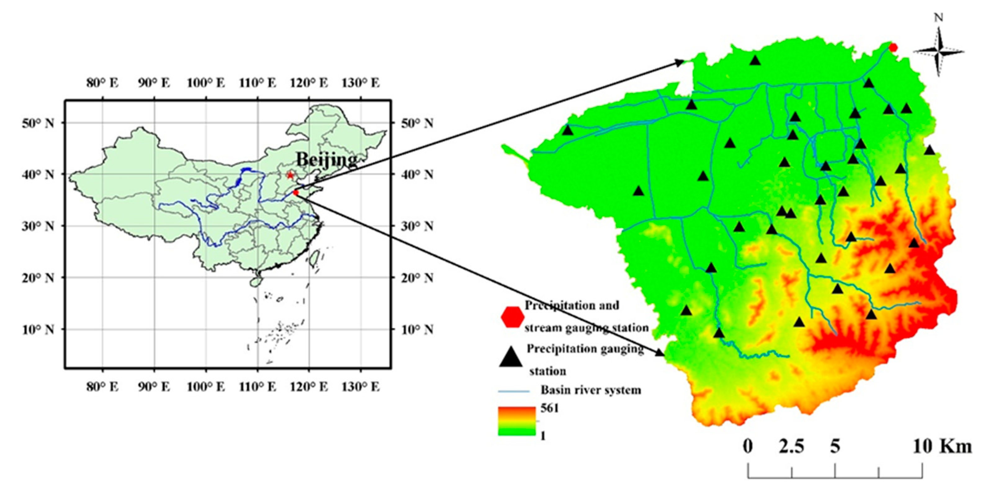
Jinan is located at the southeastern edge of North China Plain, with Mount Tai in the south and the Yellow River in the north. The terrain is high in the south and low in the north. The climate type is a temperate continental monsoon climate, and the annual average precipitation is 580–750 mm, accounting for 75% of the annual precipitation in the flood season [61]. Although the Yellow River passes through the northern part of the urban area of Jinan, Jinan does not belong to the Yellow River Basin but to the Xiaoqing River Basin, because the Jinan section of the Yellow River is an “overground river”, and the flood control dam is more than 20 m above the urban area [62]. Huangtaiqiao River basin is located in the main urban area of Jinan city, covering an area of 321 km2. Xiaoqing River is the only river flowing out of the basin and the final drainage channel of Jinan city. It originates from the northwest of Jinan city and eventually flows into the Bohai Sea. Huangtaiqiao Hydrology Station is the general control station of the Jinan urban area, located in the lower reaches of the Jinan urban section of Xiaoqing River, and the runoff of the urban river ultimately flows out through the Huangtaiqiao Hydrology Station [62]. Details of the study area are shown in Figure 1.
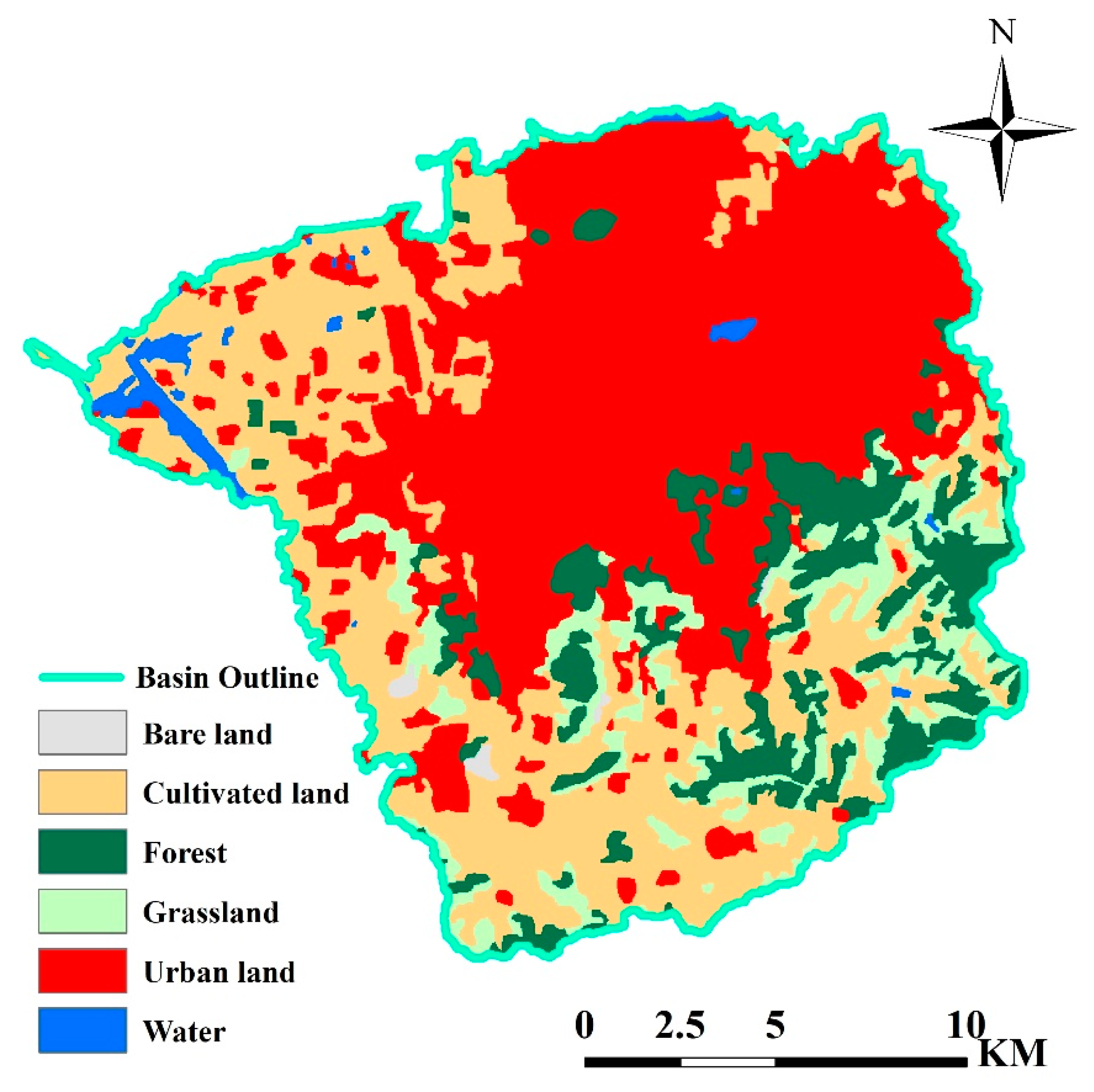
Data used in this study include rainfall, evaporation, runoff, DEM, land use, and inter-basin water transfer. Hydrological data (rainfall, evaporation, and runoff) were obtained from The Hydrological Bureau of Jinan City, including hourly precipitation data from 37 rainfall stations in the study area for 2000–2017, daily evaporation data from the study area for 2000–2017, and hourly runoff data from the Huangtaiqiao hydrological station for 2000–2017. FABDEM, from the University of Bristol (https://data.bris.ac.uk/data/dataset/ accessed on 12 May 2022), is the world’s first elevation model dataset that simultaneously removes trees and buildings [63]. The dataset is between 60° S and 80° N, and the resolution is 30 m. The land use data were obtained from 2015 Landsat remote sensing image data of Jinan city from China Geospatial Data Cloud (https://www.gscloud.cn/ accessed on 7 December 2021), with a resolution of 30 m. The data for the inter-basin water transfer are from the Hydrology Bureau of Jinan City, including data on the annual inter-basin water transfer amount and usage of inter-basin water transfer in Huangtaiqiao Basin from 2008 to 2017. The distribution of rainfall stations, hydrologic stations, and DEM in the study area is shown in Figure 1, and the land use distribution is shown in Figure 2. For the data on inter-basin water transfer, please refer to Supplementary material Table S1.
2.2. GR3
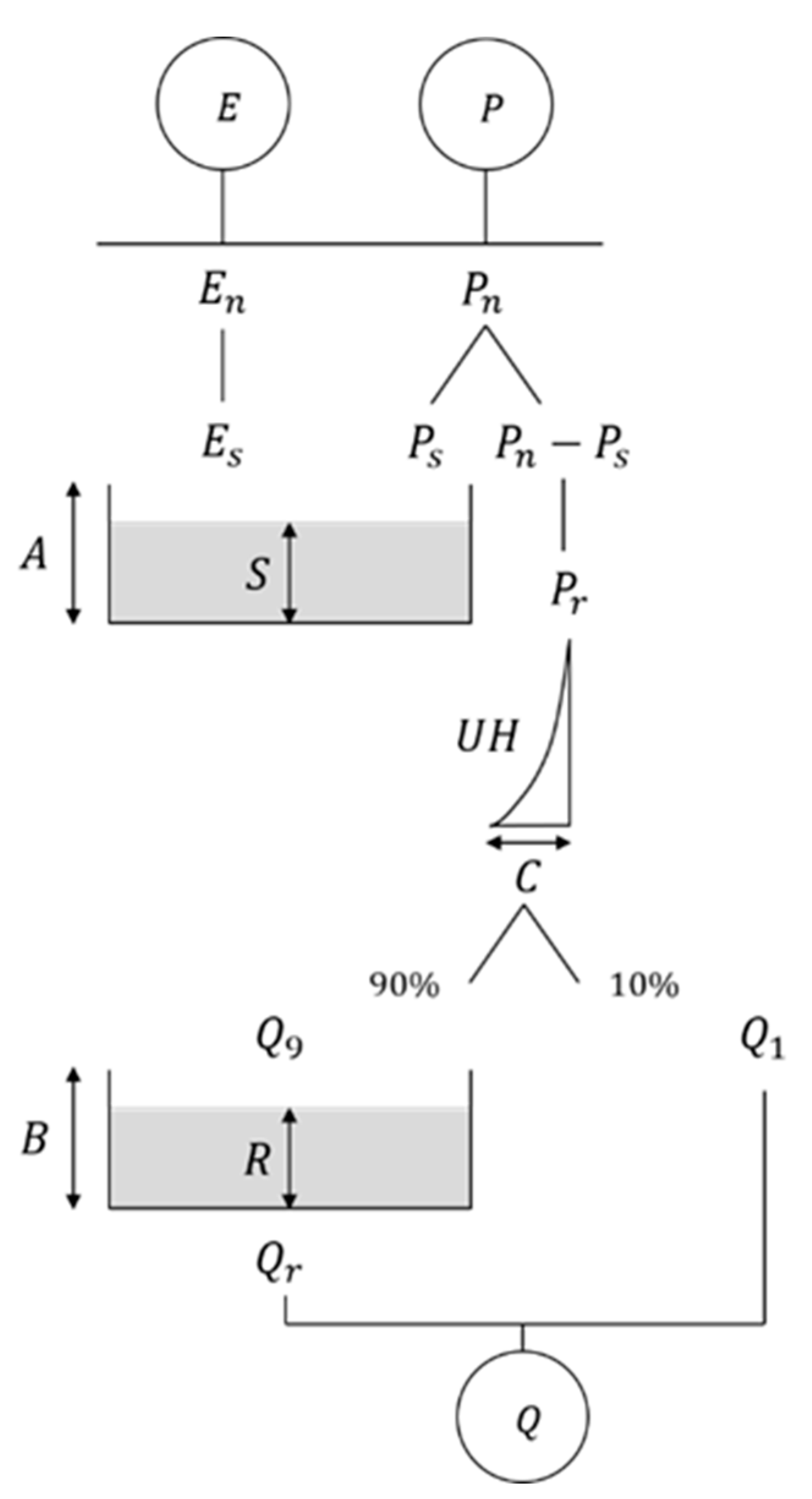
GR3 is a lumped conceptual rainfall–runoff model with three parameters. It is based on the storage, infiltration, migration, and evaporation of water in the soil, and uses empirical or semi-empirical mathematical expressions to describe the formation process of watershed runoff. The model is designed around the runoff generation tank and the runoff routing tank. The runoff generation tank reveals the storage process of soil water. The effective rainfall after deducting evaporation is calculated through the unit line of the slope after satisfying the soil water storage capacity. Part of it becomes direct runoff, and the other part enters the runoff routing tank, which is superimposed with the direct runoff after calculation. Then the outflow process is formed. The whole model is designed with three calculation units: Rainfall and evaporation calculation, runoff generation calculation, and runoff routing calculation, as shown in Figure 3.
The GR3 model contains three parameters to be optimized, namely A, B, and C (see Table 1 for details), which represent the maximum water depth of the runoff generation tank, the maximum water depth of the runoff routing tank, and the number of unit line periods, respectively. Automatic calibration can be achieved in the model. The 80% confidence interval in Table 1 is the statistical results obtained from large sample experiments in the United States, France, Australia, Ivory Coast, Brazil, and other places [64,65]. In addition, the GR3 model also includes six fixed parameters. These values are fixed after a large sample test [64,65].
2.3. Processing of Inter-Basin Water Transfer and Integration into GR3 Model
Due to data limitations, data from 2008 to 2017 were used in this study. According to the Hydrology Bureau of Jinan city, in 2000, Jinan city began to make extensive use of water transferred across the basin. Due to the lack of complete data [66] for the annual inter-basin water transfer volume from 2000 to 2007, we chose to use the minimum inter-basin water transfer data from 2008 to 2017. At the same time, we learned from the Hydrology Bureau of Jinan that all the water transferred across the basin is used for urban water in Jinan, and the daily water transferred in each water transfer cycle (every year) is average, and the water transferred is used for domestic water, industrial water, irrigation water, and river water replenishment. According to the data on inter-basin water transfer provided by The Hydrological Bureau of Jinan city (see Table 2 for details), domestic water takes up the largest proportion in these water transfer directions, and the average proportion of multi-year (water transfer cycle) reaches 37%, that is, 37% of the water transferred across basin every year (water transfer cycle) is transported to every household for urban residents. The multi-year average proportions of other water transfer destinations are 13% for irrigation, 21% for industrial use, and 29% for river replenishment.
In addition to irrigation water being directly used for agricultural irrigation and water replenishment directly into rivers, domestic water and industrial water are transported to households and factories through water distribution networks. Some of the water enters the river from the sewer, and some of the water is treated by the sewage treatment plant and then enters the river. As a result, in a short time scale (1 h), there is a certain lag between the introduction of inter-basin water transfer and the use of inter-basin water transfer. According to the Jinan Statistical Yearbook, the Jinan Water Resources Bulletin, and related studies [67,68,69], the average daily water consumption in the study area tends to be stable for many years. Therefore, in the long time scale used here (18 years), the lag between the introduction of inter-basin water transfer and the use of inter-basin water transfer has little impact on the study and is therefore ignored in this study. Some of the urban water is reused through recycling [70,71]. According to the Jinan Water Resources Bulletin, the average comprehensive water consumption rate in the study area for years is 70%, that is, 30% of the water has been reused. This study did not integrate this part of the reused water into the rainfall and runoff model. Since more specific industry water consumption rates were not found, the study no longer distinguished between them. Land use distribution can roughly reflect the destination distribution of inter-basin water transfer [67,68,69,72]. It can be seen from Figure 1 and Figure 2 that construction land, cultivated land, and river channels are widely distributed in the study area, so this study does not show special treatment for the destination distribution of inter-basin water transfer.
2.3.1. Downscaling of Inter-Basin Water Transfer
The section above points out that the daily water transfer volume is the average in the inter-basin water transfer cycle (every year). In order to unify the time scale of inter-basin water transfer data and hydrological data (precipitation, evaporation, and runoff), the annual water transfer volume is converted into an hourly water transfer volume through the following formula:
In the formula, is the hourly inter-basin water transfer volume ) and is the annual inter-basin water transfer volume ). Considering that the inter-basin water transfer volume should be integrated into the GR3 model and combined with the multi-year average comprehensive water consumption rate in the basin, the hourly inter-basin water transfer volume (m³) was converted into the hourly inter-basin water transfer depth (mm) by the following formula:
In the formula, is the hourly inter-basin water transfer depth ) is the multi-year average comprehensive water consumption rate (%), and is the basin area (. We allocate according to the proportion of water transfer purposes to obtain the hourly inter-basin water transfer depth for different purposes.
2.3.2. Integrating Inter-Basin Water Transfer into GR3
The hourly inter-basin water transfer depth for different purposes is calculated in Section 2.3.1. To integrate the inter-basin water transfer into the GR3 model, in addition to the data scale problem already solved in Section 2.3.1, two aspects should be considered, namely, the GR3 model structure and the use characteristics of water transfer for different purposes. From Section 2.2, it can be seen that the GR3 model includes three units: Rainfall and evaporation calculation, runoff generation calculation, and runoff routing calculation. While the inter-basin water transfer is integrated into the model, it is also necessary to analyze the use characteristics of water transfer for different purposes. As mentioned above, domestic water and industrial water are transported to each water-using unit through the water pipe network. After using the water, the water-using unit discharges it into the sewer, and then enters the river for routing. Therefore, the domestic and industrial water is integrated into the river routing part of the GR3 model and participate in the model calculation together with the amount of runoff generation (). Irrigation water is transported to farmland for irrigation through the water pipe network. During irrigation, irrigation water will undergo evaporation and infiltration, followed by runoff generation and routing. These processes are similar to the “rain–runoff” process in the natural state. Therefore, irrigation water is integrated into the rainfall and evaporation part of the GR3 model and participates in the model calculation together with the precipitation (). The river water replenishment directly flows into the river through the water pipe network, and then converges to the outlet of the basin through the river network. Therefore, the river water replenishment is integrated into the runoff routing part of the GR3 model and participates in the model calculation together with the amount of runoff generation (). The specific process is shown in Figure 4.
2.4. Model Setup and Data Processing
Continuous hydrological simulations for 18 years (2000–2017) were performed using the GR3 model and the GR3-ibwt model, respectively, with a time resolution of 1 h. Parameter calibration was performed using the minimum square error function (MSE). From the input side of the model, the time resolution of rainfall and runoff data in the hydrological data meets the simulation requirements; the evaporation data are daily evaporation, which needs to be processed to ensure the time resolution meets the simulation requirements. Evaporation changes more gradually over time than rainfall, so linear interpolation is performed on the daily evaporation data to meet the simulation requirements. From the perspective of the watershed distribution, the evaporation data obtained are the average data of the research area, so the evaporation data distribution is not processed; rainfall data come from all rainfall stations (including the Huangtaiqiao hydrological station). There are a large number (37) of rainfall stations in the study area, with uniform distribution, and the area of the study area is small (321 km2). Therefore, the average value of measured data from all rainfall stations is calculated as the input data of the model. The data processing of inter-basin water transfer is detailed in Section 2.3 and will not be repeated here.
In this study, the hydrological simulation data volume is large, the time series is long (18 years), and the time resolution is high (1 h). Compared with the daily-scale (1d) simulation, more flood information can be captured. The period of 2000–2003 was used as the model warm-up period, 2004–2010 was the model calibration period, and 2011–2017 was the model validation period. According to the observed flood peak flow, the floods in the study area are divided into three levels: Big floods (peak flow > 130 m3/s), medium floods (80 m3/s < peak flow < 130 m3/s), and small floods (peak flow < 80 m3/s). The simulation results of 21 floods of different sizes in the long-term series simulation results were selected for statistical analysis for the single-flood process test. The selected single-flood process is shown in Table 3.
2.5. Model Evaluation Methods
In this paper, the performance of the model is evaluated on two scales, a long time series (18 years) and a single-flood process. The Nash–Sutcliffe efficiency coefficient (NSE) and the water relative error (RE) are selected as the long-term simulation evaluation indicators [73,74]; the Nash–Sutcliffe efficiency coefficient (NSE), the relative error of water volume (RE), the relative error of flood peak flow (PE), and difference in peak arrival time (DPAT) were selected as evaluation indicators for single-flood process simulation [75]. The calculation formula of each index is as follows:
In the formula is the simulated discharge ) is the observed discharge () is the averaged observed discharge (), is the simulated peak discharge (), is the observed peak discharge (), is the arrival time of the simulated peak discharge , and is the arrival time of the observed peak discharge .
The resulting range of the Nash–Sutcliffe efficiency coefficient (NSE) is , whereby the closer it is to 1, the better the model simulation effect is. Generally, the model simulation effect is acceptable if it is above 0.5. The closer the relative error of water flow (RE) and flood peak flow (PE) are to 0, the better the simulation effect of the model will be. Generally, a range of indicates that the simulation effect of the model is acceptable [73,74,75].
3. Results
3.1. Long-Time Series Simulation Results
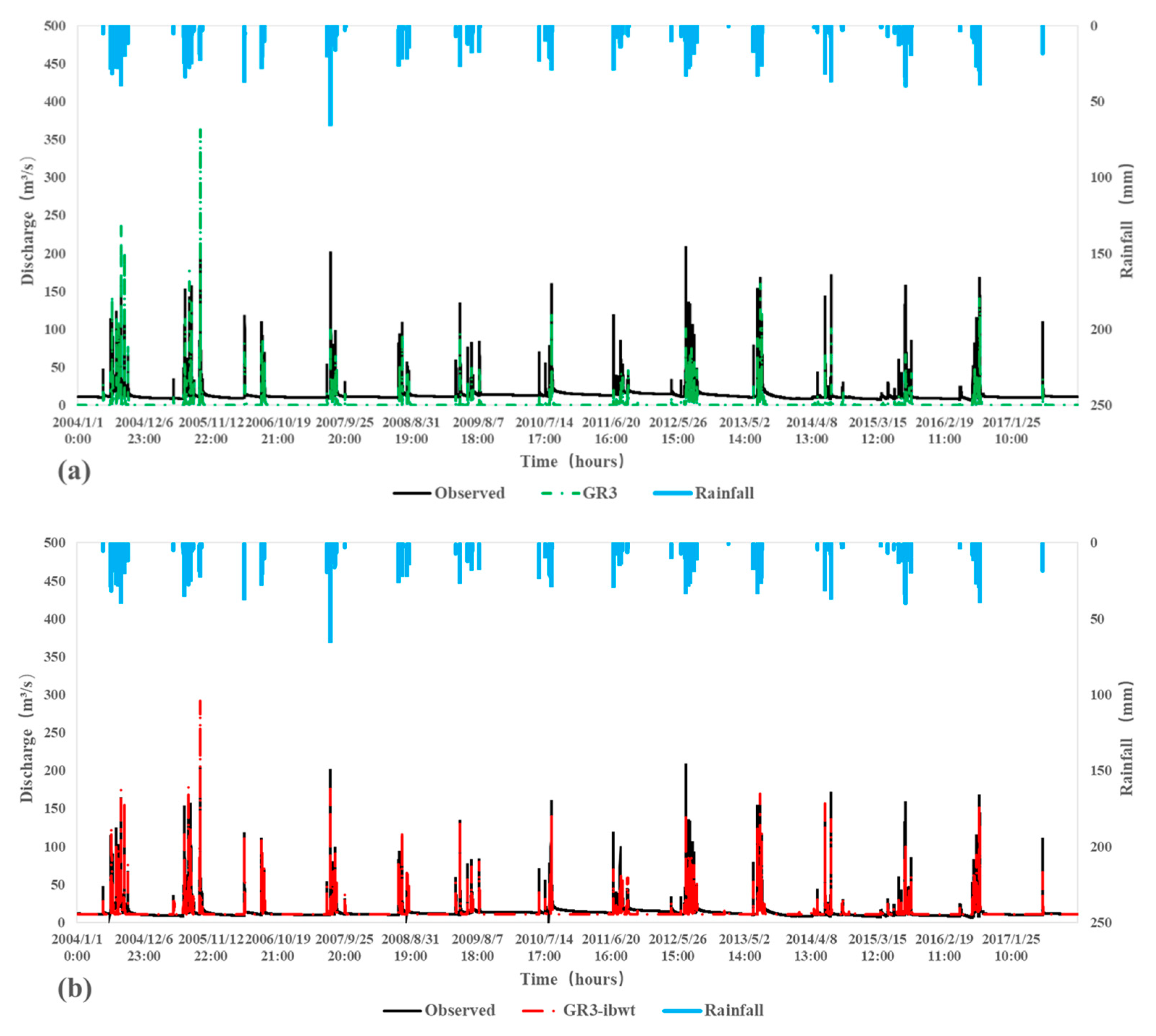
In this study, continuous hydrological simulations for 18 years (2000–2017) were performed using the GR3 model and the GR3-ibwt model, respectively, with a time resolution of 1 h. Among them, 2000–2003 is the model warm-up period, 2004–2010 is the model calibration period, and 2011–2017 is the model validation period. Excluding the warm-up period, the simulated runoff and the observed runoff at the outlet of the basin during the model calibration period and validation period are shown in Figure 5. It can be seen from the figure that compared with the observation process, the simulation results of the GR3 model are poor, and most of the simulated flood peaks are far away from the measured peaks. The simulated runoff in the drought period is close to 0, and the observed runoff is generally higher than the simulated runoff. The reason for this phenomenon is that the GR3 model is a rainfall–runoff model. Without considering the inter-basin water transfer, the model runoff is mainly related to the rainfall and evaporation of the basin [64,65]. When there is no rainfall, the runoff will not be generated. Due to the existence of inter-basin water transfer, the runoff can be observed at the outlet of the basin when no rainfall occurs. At the same time, long-term inter-basin water transfer has an impact on the nature of the underlying surface of the basin to a certain extent [76], which is mainly reflected in the change in soil moisture [45,77,78], which will affect the performance of the GR3 model and increase the error in runoff generation calculations. Compared with a single flood, the impact of cross-basin water transfer on the long-term series simulation is magnified. Therefore, this paper chooses to use long-term hydrological data for the simulation and selects the single-flood simulation results for statistical analysis. The purpose of this is to consider the long-term impact of inter-basin water transfer on the one hand, and on the other hand, the long-term series simulation will reduce the pseudo precision caused by direct single-flood simulation.
Compared with GR3, the simulated process of the GR3-ibwt model is closer to the observed process. From the flood peak simulation results, the GR3-ibwt model can simulate the flood peak flow well in most flood peaks, and only a few flood peaks have large simulation errors, which is greatly improved compared with the GR3 model simulation results. From the simulation results of the dry season, the simulation process of the GR3-ibwt model is almost identical to the observation process, which is a qualitative improvement compared with the simulation results of the GR3 model. It can be seen that when the inter-basin water transfer is considered, the study area achieved a water balance, and the urban basin with a high concentration of population is equivalent to a natural basin without human interference to a certain extent, and the simulation results of the rainfall–runoff model are generally better.
In order to further evaluate the performance of the model, the Nash–Sutcliffe efficiency coefficient (NSE) and the water relative error (RE) in the calibration and verification periods of the two hydrological simulations were calculated. The results are shown in Table 4, and the model parameters are shown in Table S2 of Supplementary Materials.
It can be seen that the Nash-Sutcliffe efficiency coefficient (NSE) of the GR3 model is far less than 0 in both the calibration period and the verification period, which is far from the lower limit of acceptability of 0.5, indicating that the simulation results are not credible. The relative error (RE) of water volume is below −0.85, which means that the simulated runoff is much smaller than the observed runoff, which is consistent with Figure 4. The Nash-Sutcliffe efficiency coefficients (NSE) of the GR3-ibwt model were 0.77 and 0.70 in the calibration period and validation period, respectively, and the model performance reached a good level [73,74,75]. Compared with the GR3 model, the Nash–Sutcliffe efficiency coefficients (NSE) increased by 178% and 142%, respectively. The water relative errors (RE) in the calibration period and validation period were −0.06 and −0.04, respectively, indicating that the simulated water volume of the GR3-ibwt model essentially reached a water balance with the actual observed water volume, and the water relative errors (RE) decreased by 94% and 96% compared with the GR3 model, respectively. Overall, the Nash–Sutcliffe efficiency coefficient (NSE) results of the GR3-ibwt model in the long-term series simulation essentially reached a good level, and the water balance was above 94%. Compared with the GR3 model, the results of the two indicators were significantly improved. From the perspective of a long time series, the hydrological simulation using the rainfall–runoff model without considering inter-basin water transfer is not in line with the actual situation, and the simulation results are greatly different from the measured process. Integrating the inter-basin water transfer into the rainfall–runoff model for hydrological simulation is closer to the actual situation, and the simulation results are relatively satisfactory.
3.2. Single Flood Simulation Results
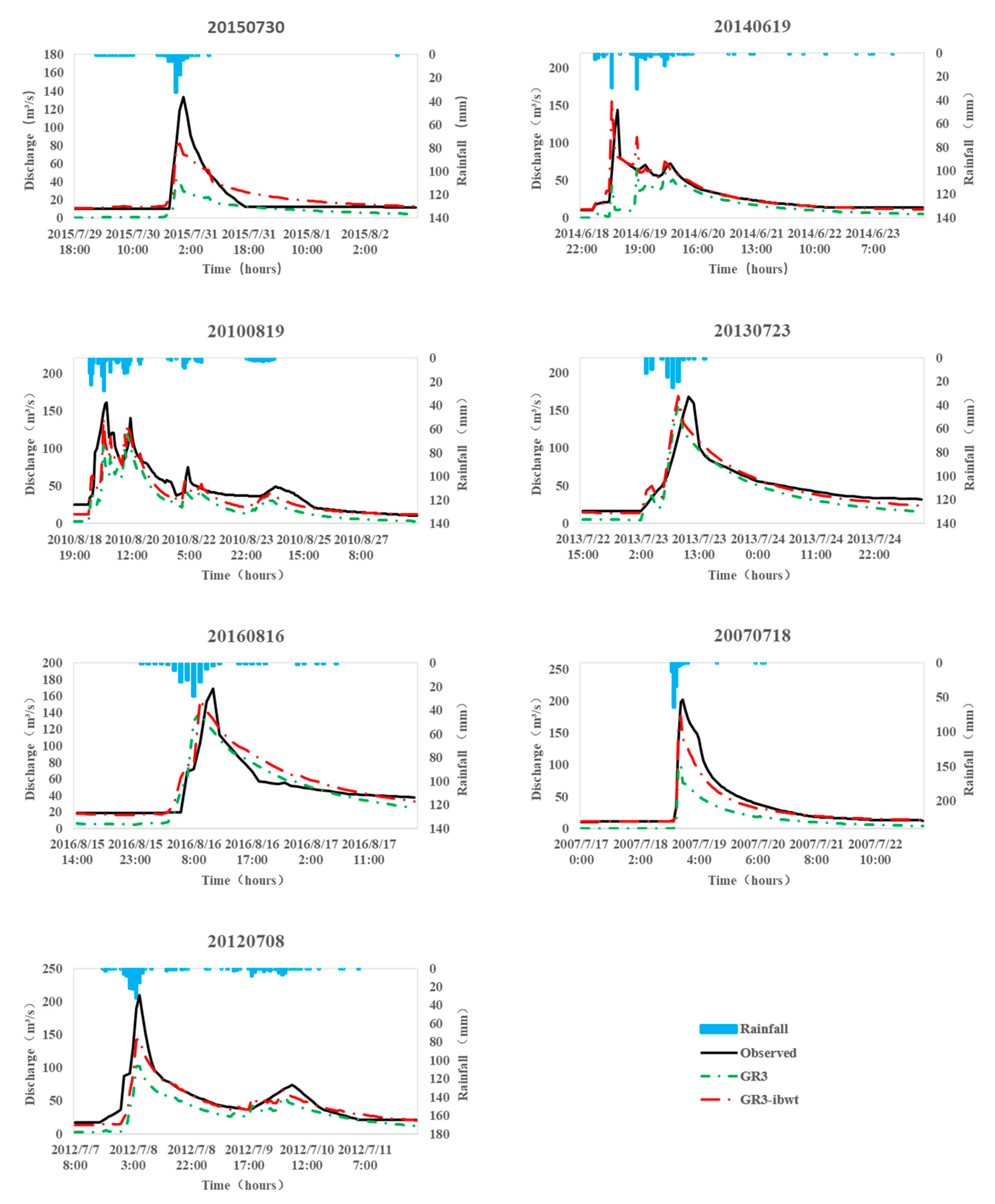
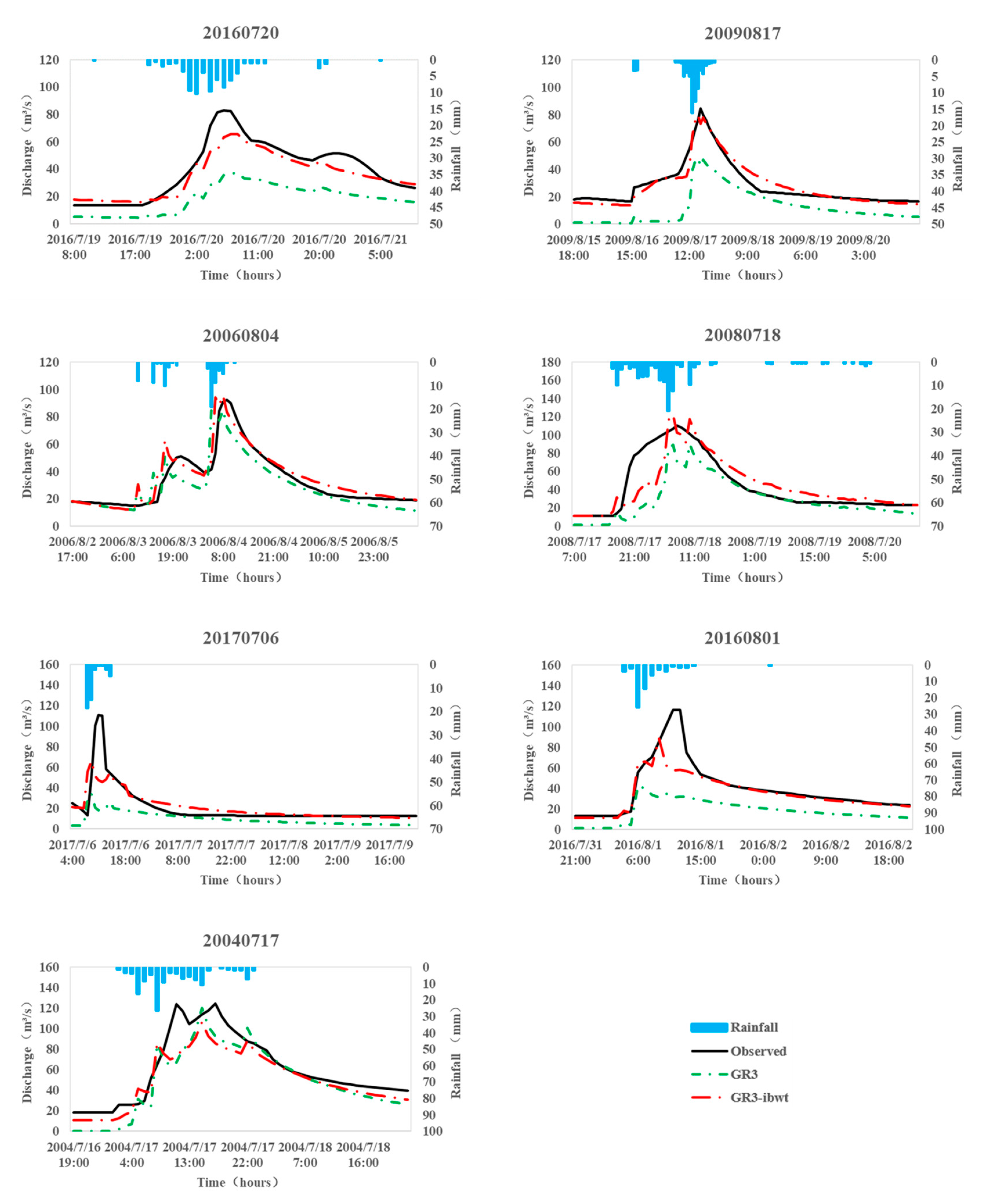
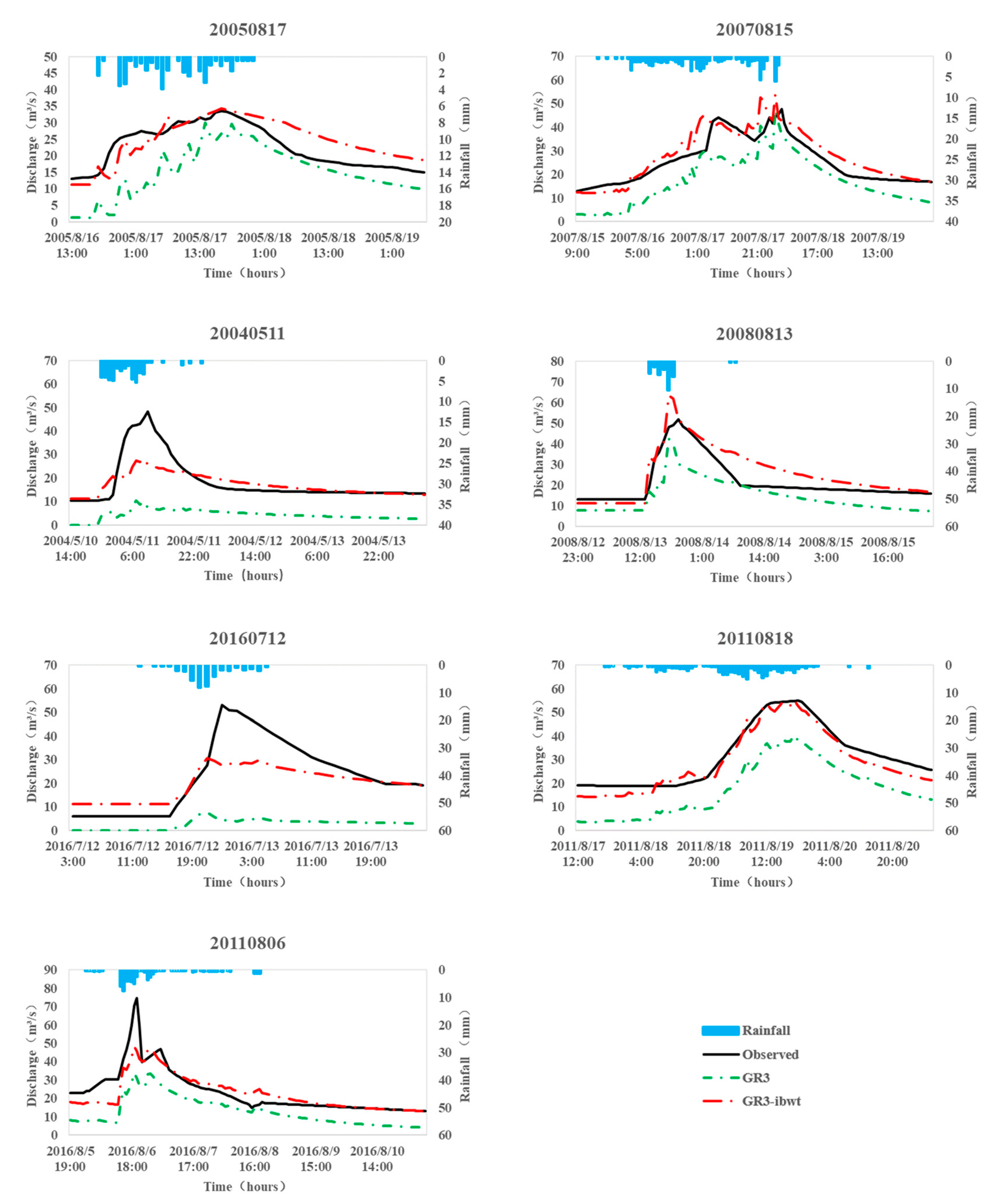
In order to reduce the pseudo precision brought by the direct simulation of a single flood, 21 flood simulation results of different scales in the long-term series (see Table 3 for details) were selected for statistical analysis. According to the observed flood peak flow, the flood in the study area is divided into three levels: Big floods (peak flow > 130 m3/s), medium floods (80 m3/s < peak flow < 130 m3/s), and small floods (peak flow < 80 m3/s). Figure 6, Figure 7 and Figure 8 show the simulated runoff of big, medium, and small floods and the observed runoff at the basin outlet, respectively.
It can be seen from Figure 6 that the GR3 model has a general performance in the simulation of big floods, with good performance only in 20100819, 20130723, and 20160816, and poor performance in the other four floods. The GR3-ibwt model has a good overall performance in the simulation of big floods, which is slightly better than the GR3 model in 20100819, 20130723, and 20160816. The performance of the other four floods is significantly improved compared with the GR3 model.
As can be seen from Figure 7, the GR3 model has poor overall performance in the simulation of medium floods, with good performance only in the flood of 20060804 and poor performance in the other six floods. The GR3-ibwt model has a general performance in the simulation of medium floods, with good performance in 20090817, 20060804, and 20080718, while the other floods have a general performance, which is greatly improved compared with the GR3 model.
As can be seen from Figure 8, the GR3 model has poor overall performance in the simulation of small floods, and the performance of each flood is not satisfactory. The GR3-ibwt model has a general overall performance in the simulation of small floods, with good performance in the three floods of 20050817, 20070815, and 20110818. Although the performance of other floods is average, it is greatly improved compared with the GR3 model.
To summarize, the GR3 model and the GR3-ibwt model have similar performances in the single-flood scale from the basin outlet flow process diagram, that is, the simulation results of big floods are better than those of medium and small floods.
In order to further evaluate the model performance, the Nash–Sutcliffe efficiency coefficient (NSE), water relative error (RE), the relative error of flood peak flow (PE), and difference of peak arrival time (DPAT) of each flood simulation for the GR3 model and the GR3-ibwt model were calculated, respectively. The results are shown in Table 5. As can be seen from Table 5, (1) for the simulation of flood peak flow, the GR3-ibwt model is better than the GR3 model on the whole and closer to the observed flow. (2) For the Nash–Sutcliffe efficiency coefficient (NSE), the overall performance of the GR3-ibwt model is better than the GR3 model, with two floods above 0.9, 14 floods above 0.7, all floods above 0.5, and the performance of large floods is better than medium and small floods. (3) For the relative error of water volume (RE), the overall performance of the GR3-ibwt model is better than that of the GR3 model, and the relative error of water volume in all floods is within 0.2. (4) For the relative error of flood peak flow (PE), the overall performance of the GR3-ibwt model is better than that of the GR3 model. There are 12 flood peak flow relative errors within 0.2, and the maximum flood peak flow relative error is 0.42 (two floods). (5) For the difference in peak arrival time (DPAT), the overall performance of the GR3-ibwt model is better than the GR3 model, and the maximum difference in peak arrival time in all flood events does not exceed 2 h.
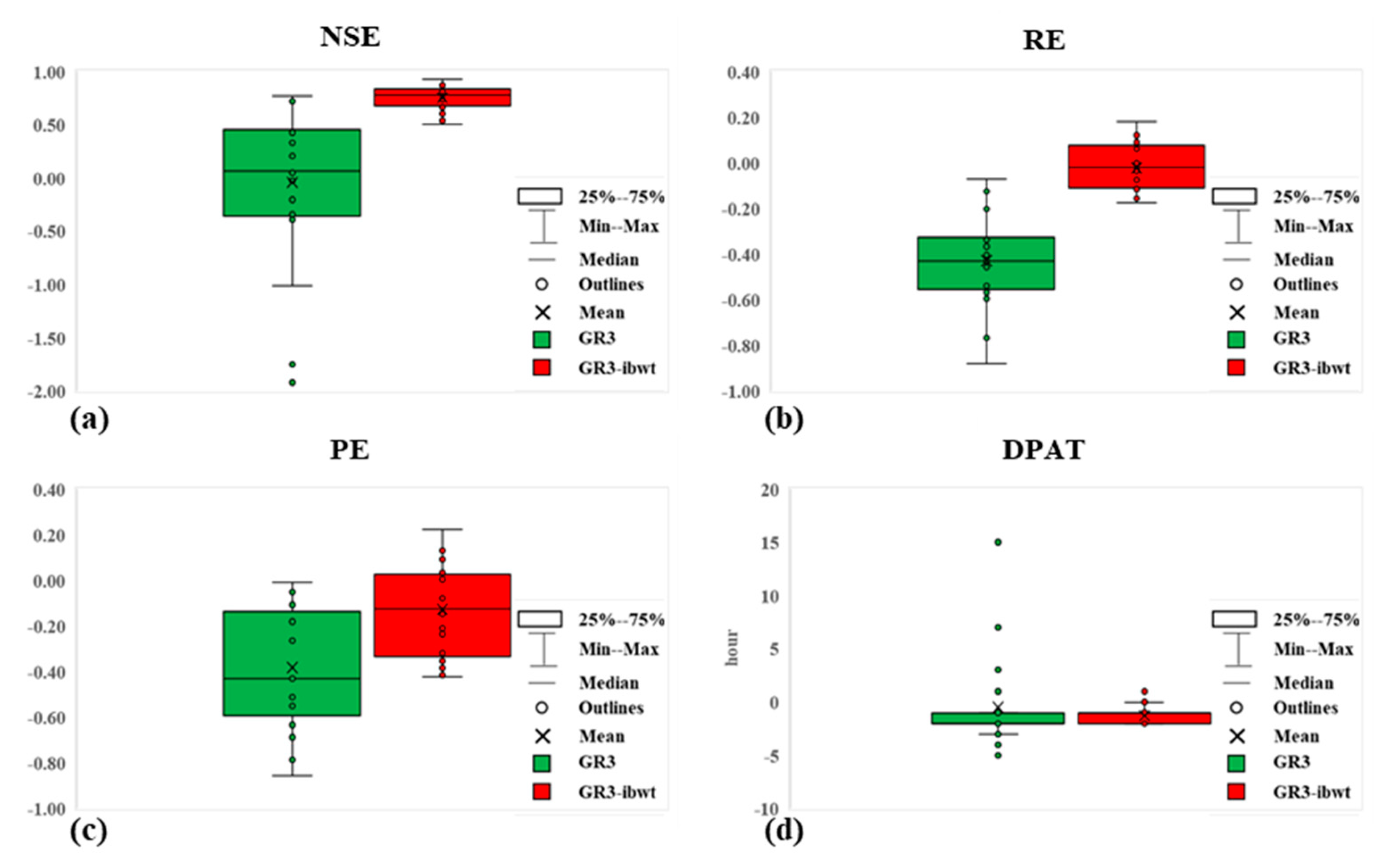
Statistical analysis was carried out on the four model evaluation indicators of all simulated flood events of the GR3 model and the GR3-ibwt model (See Figure 9 for details). As can be seen from Figure 9a, the Nash–Sutcliffe efficiency coefficient (NSE) of the GR3-ibwt model was greatly improved compared with the GR3 model, and the fluctuation range changed from [−1.01, 0.77] to [0.50, 0.92], and the median and mean increased from 0.07 and −0.04 to 0.78 and 0.75, respectively, and there was no abnormally low value. As can be seen from Figure 9b, the water relative error (RE) of the GR3-ibwt model was greatly reduced compared with the GR3 model, and the fluctuation range changed from [−0.88, −0.07] to [−0.18, 0.18]. Both the median and mean changed from −0.43 to −0.02. As can be seen from Figure 9c, the peak discharge relative error (PE) of the GR3-ibwt model is significantly lower than that of the GR3 model, and the fluctuation range changes from [−0.86, −0.01] to [−0.42, 0.22], while the median and mean changed from −0.43 and −0.38 to −0.13 and −0.13, respectively. As can be seen from Figure 9d, the difference in peak arrival time of the GR3-ibwt model is significantly lower than that of the GR3 model, and there are a large number of abnormal values in the different peak arrival times of the GR3 model. For the separate statistics of the model evaluation indicators of small, medium, and big floods, see Figures S1–S3 in the Supplementary Materials.
4. Discussion
In general, the GR3-ibwt model had better simulation results than the GR3 model in both long time series scale and single flood scale, and the results are relatively satisfactory. Specifically, for the simulation of the long time series, the Nash-Sutcliffe efficiency coefficient (NSE) of the GR3-ibwt model was increased by 178% and 142% in the calibration and validation periods, respectively, compared with the GR3 model. At the same time, the water relative error (RE) was reduced by 94% and 96% compared with the GR3 model during the calibration period and the validation period, respectively. Both model evaluation indicators prove that the GR3-ibwt model has good simulation performance on long time scales. The reason is that the GR3-ibwt model considers the inter-basin water transfer based on the GR3 model, and the rainfall–runoff simulation of the basin achieves a water balance and reduces the long-term impact of inter-basin water transfer on the hydrological effect of the basin.
For the simulation of the single-flood scale, the performance of the GR3-ibwt model is better than that of the GR3 model in four evaluation indicators: Nash–Sutcliffe efficiency coefficient (NSE), water relative error (RE), peak discharge relative error (PE), and difference of peak arrival time (DPAT). The simulation of big floods is better than that of medium and small floods. The reason is that in urban flood simulation, precipitation still plays a leading role [35,36], and big floods are less affected by other disturbances, which can be confirmed by the GR3 model’s overall simulation of big floods also performing better than that of medium and small floods. Regarding the time lag of the flood peak, we suggest this is because the properties of the underlying surface (such as soil water requirement) of the basin change under the action of inter-basin water transfer over a long period of time, which makes it less sensitive to the flood peak. The results prove that this is more consistent with reality.
Hydrological simulation of urban basins is very common at present, but the phenomenon of inter-basin water transfer is rarely considered. However, the phenomenon of inter-basin water transfer is now very common, especially in urban basins where water resources are scarce. Therefore, the fundamental difference between this paper and other studies in this field is that the factor of inter-basin water transfer is taken into account in the hydrological simulation. We chose Jinan, the capital of Shandong Province in China, as the study area, which is an important city in East China. At the same time, the data we used are real data provided by local departments rather than scenario analysis, so we believe that this study reflects reality to a certain extent, both in terms of representativeness of the study area and data reliability. The biggest limitation of this study is the acquisition of measured data. On the one hand, high-precision hydrological data are required, and on the other hand, inter-basin water transfer data within the same period are also required, while at the same time, different uses of inter-basin water transfer are required. Once these data are obtained, they can be processed and combined with different types of hydrological models for hydrological simulations.
This study attempts to integrate the inter-basin water transfer into the rainfall–runoff model, and the results are relatively satisfactory. Subsequent research can focus on the following aspects: (1) Conducting a more comprehensive analysis of inter-basin water transfer so that it can be better integrated into the rainfall–runoff model, such as further refinement of the temporal and spatial distribution of inter-basin water transfer, and more comprehensive analysis of the use of inter-basin water transfer. Furthermore, researchers should (2) perform hydrological simulations under the background of inter-basin water transfer in other urban basins with data support and compare this with hydrological simulation results that do not consider inter-basin water transfer. Moreover, (3) the GR3-ibwt model could be applied to urban water resource management, urban water landscape design, basin ecological protection, and other aspects. Lastly, (4) by coupling the GR3-ibwt model with the hydraulic model and replacing the runoff routing part of the GR3-ibwt model with the hydraulic model for the simulation, one can obtain more flood information that has more physical meaning.
5. Conclusions
In this study, a new urban hydrological simulation method was proposed. Based on the GR3 rainfall–runoff model, the inter-basin water transfer is processed and integrated into the GR3 model, and then the hydrological simulation is conducted. The study area is located in the Huangtaiqiao basin of Jinan City, Shandong Province, China. The simulation object is the hydrological data of the Huangtaiqiao basin from 2000 to 2017, with a time resolution of 1 h, and 21 flood simulation results of different scales were selected for statistical analysis. By comparing the simulated results of the GR3-ibwt model with those of the GR3 model and measured data, their performances on the Nash–Sutcliffe efficiency coefficient (NSE), water relative error (RE), peak discharge relative error (PE), and difference peak arrival time (DPAT) were evaluated on the two scales of a long time series (18 years) and a single flood (21 flood events). The following conclusions are drawn:
(1) The GR3-ibwt model performs well in the hydrological simulation of an urban basin, and the long-term series and single-flood simulation results are satisfactory. (2) We demonstrate that inter-basin water transfer has a long-term impact on the rainfall–runoff process of urban basins and provide a new perspective and method for long-term hydrological simulation of urban basins. We also (3) revealed the potential application of the GR3-ibwt model in urban water resource management, urban water landscape design, basin ecological protection, and other aspects. Lastly, we (4) suggested the necessity of and made recommendations for further research.
Supplementary Materials
The following supporting information can be downloaded at: https://www.mdpi.com/article/10.3390/w14172660/s1, Table S1. The volume of inter-basin water transfer in Huangtaiqiao basin; Table S2. The parameters of GR3 and GR3-ibwt; Figure S1. Box diagram of the measured and simulated discharge evaluation in small flood processes; Figure S2. Box diagram of the measured and simulated discharge evaluation in medium flood processes; Figure S3. Box diagram of the measured and simulated discharge evaluation in big flood processes.
Author Contributions
Conceptualization, J.Y. and C.X.; methodology, J.Y.; software, J.Y.; validation, J.Y. and C.X.; formal analysis, J.Y.; investigation, J.Y., C.X., X.N. and X.Z.; resources, J.Y.; data curation, J.Y.; writing—original draft preparation, J.Y.; writing—review and editing, C.X. and X.N.; visualization, J.Y.; supervision, J.Y.; project administration, J.Y. All authors have read and agreed to the published version of the manuscript.
Funding
This paper was funded by the Major Science and Technology Program for Water Pollution Control and treatment, China (Grant No. 2014ZX07203-008).
Institutional Review Board Statement
Not applicable.
Informed Consent Statement
Not applicable.
Data Availability Statement
Not applicable.
Acknowledgments
We acknowledge the continued support and generosity of Xiaoliu Yang from the College of Urban and Environmental Sciences, Peking University. This work was financially supported by the Major Science and Technology Program for Water Pollution Control and treatment, China (Grant No. 2014ZX07203-008).
Conflicts of Interest
The authors declare no conflict of interest. The funders had no role in the design of the study; in the collection, analyses, or interpretation of data; in the writing of the manuscript, or in the decision to publish the results.
References
- Schneider, R.L. Integrated, watershed-based management for sustainable water resources. Front. Earth Sci. China 2010, 4, 117–125. [Google Scholar]
- Oki, T.; Kanae, S. Global hydrological cycles and world water resources. Science 2006, 313, 1068–1072. [Google Scholar] [PubMed]
- Hashem, M.S.; Qi, X. Treated Wastewater Irrigation—A Review. Water 2021, 13, 1527. [Google Scholar]
- Wang, J.; Hou, B.; Jiang, D.; Xiao, W.; Wu, Y.; Zhao, Y.; Zhou, Y.; Guo, C.; Wang, G. Optimal Allocation of Water Resources Based on Water Supply Security. Water 2016, 8, 237. [Google Scholar]
- Dou, X. China’s inter-basin water management in the context of regional water shortage. Sustain. Water Resour. Manag. 2018, 4, 519–526. [Google Scholar]
- Li, T.; Qiu, S.; Mao, S.; Bao, R.; Deng, H. Evaluating Water Resource Accessibility in Southwest China. Water 2019, 11, 1708. [Google Scholar] [CrossRef]
- Geng, Q.; Liu, H.; He, X.; Tian, Z. Integrating Blue and Green Water to Identify Matching Characteristics of Agricultural Water and Land Resources in China. Water 2022, 14, 685. [Google Scholar]
- Di, D.; Wu, Z.; Guo, X.; Lv, C.; Wang, H. Value Stream Analysis and Emergy Evaluation of the Water Resource Eco-Economic System in the Yellow River Basin. Water 2019, 11, 710. [Google Scholar] [CrossRef]
- Song, P.; Wang, C.; Zhang, W.; Liu, W.; Sun, J.; Wang, X.; Lei, X.; Wang, H. Urban Multi-Source Water Supply in China: Variation Tendency, Modeling Methods and Challenges. Water 2020, 12, 1199. [Google Scholar]
- Hattingh, J.; Maree, G.A.; Ashton, P.J.; Leaner, J.J.; Rascher, J.; Turton, A.R. Introduction to ecosystem governance: Focusing on Africa. Water Policy 2007, 9, 5–10. [Google Scholar]
- Su, D.; Zhang, Q.H.; Ngo, H.H.; Dzakpasu, M.; Guo, W.S.; Wang, X.C. Development of a water cycle management approach to Sponge City construction in Xi’an, China. Sci. Total Environ. 2019, 685, 490–496. [Google Scholar] [PubMed]
- Sun, W.; Ren, J.M. Development and Utilization Status in the Basin of Shiyang River and Water Quality Evaluation. Appl. Mech. Mater. 2012, 212, 482–486. [Google Scholar] [CrossRef]
- Ni, L.; Fan, M.; Qu, S.; Zheng, Q. Based on GMS management of shallow groundwater resource in Ningjin, China. IOP Conf. Ser. Earth Environ. Science 2019, 237, 32063. [Google Scholar] [CrossRef]
- Li, F.; Yan, W.; Zhao, Y.; Jiang, R. The regulation and management of water resources in groundwater over-extraction area based on ET. Theor. Appl. Climatol. 2021, 146, 57–69. [Google Scholar]
- Jia, X.; O’Connor, D.; Hou, D.; Jin, Y.; Li, G.; Zheng, C.; Ok, Y.S.; Tsang, D.C.W.; Luo, J. Groundwater depletion and contamination: Spatial distribution of groundwater resources sustainability in China. Sci. Total Environ. 2019, 672, 551–562. [Google Scholar]
- Wang, H.; Wang, Y.; Jiao, X.; Qian, G. Risk management of land subsidence in Shanghai. Desalin. Water Treat. 2014, 52, 1122–1129. [Google Scholar]
- Fan, Y.; Lu, W.; Miao, T.; Li, J.; Lin, J. Multiobjective optimization of the groundwater exploitation layout in coastal areas based on multiple surrogate models. Environ. Sci. Pollut. R 2020, 27, 19561–19576. [Google Scholar]
- Bozorg-Haddad, O.; Abutalebi, M.; Chu, X.; Loáiciga, H.A. Assessment of potential of intraregional conflicts by developing a transferability index for inter-basin water transfers, and their impacts on the water resources. Environ. Monit. Assess 2019, 192, 40. [Google Scholar] [PubMed]
- Zhang, C.; Wang, G.; Peng, Y.; Tang, G.; Liang, G. A Negotiation-Based Multi-Objective, Multi-Party Decision-Making Model for Inter-Basin Water Transfer Scheme Optimization. Water Resour. Manag. 2012, 26, 4029–4038. [Google Scholar]
- Wang, Q.; Zhou, H.; Liang, G.; Xu, H. Optimal Operation of Bidirectional Inter-Basin Water Transfer-Supply System. Water Resour. Manag. 2015, 29, 3037–3054. [Google Scholar] [CrossRef]
- Wang, Q.W.; Sun, R.R.; Guo, W.P. Study on Three-Dimensional Visual Simulation for Inter-Basin Water Transfer Project. Appl. Mech. Mater. 2013, 256, 2523–2527. [Google Scholar] [CrossRef]
- Zhang, L.; Li, S.; Loáiciga, H.A.; Zhuang, Y.; Du, Y. Opportunities and challenges of interbasin water transfers: A literature review with bibliometric analysis. Scientometrics 2015, 105, 279–294. [Google Scholar]
- Essenfelder, A.H.; Giupponi, C. A coupled hydrologic-machine learning modelling framework to support hydrologic modelling in river basins under Interbasin Water Transfer regimes. Environ. Modell. Softw. 2020, 131, 104779. [Google Scholar]
- Woo, S.; Kim, S.; Lee, J.; Kim, S.; Kim, Y. Evaluating the impact of interbasin water transfer on water quality in the recipient river basin with SWAT. Sci. Total Environ. 2021, 776, 145984. [Google Scholar] [PubMed]
- Tien Bui, D.; Talebpour Asl, D.; Ghanavati, E.; Al-Ansari, N.; Khezri, S.; Chapi, K.; Amini, A.; Thai Pham, B. Effects of Inter-Basin Water Transfer on Water Flow Condition of Destination Basin. Sustainability 2020, 12, 338. [Google Scholar] [CrossRef]
- Cao, Y.; Chang, J.; Huang, Q.; Chen, X.; Chen, Y. Study of Discharge Model in South-to-North Water Diversion Middle Route Project Based on Radial Basis Function Neural Network. MATEC Web Conf. 2016, 68, 14011. [Google Scholar] [CrossRef]
- Zhang, Y.; Li, G. Influence of south-to-north water diversion on major cones of depression in North China Plain. Environ. Earth Sci. 2014, 71, 3845–3853. [Google Scholar] [CrossRef]
- Guo, Y.C.; Li, J.F.; Li, J.L. Agent Construction System Application and Improvement Discussion in the South-to-North Water Diversion Project. Appl. Mech. Mater. 2012, 105, 1096–1099. [Google Scholar] [CrossRef]
- Arthington, A.H.; Pusey, B.J. Flow restoration and protection in Australian rivers. River Res. Appl. 2003, 19, 377–395. [Google Scholar]
- Qin, G.; Liu, J.; Wang, T.; Xu, S.; Su, G. An Integrated Methodology to Analyze the Total Nitrogen Accumulation in a Drinking Water Reservoir Based on the SWAT Model Driven by CMADS: A Case Study of the Biliuhe Reservoir in Northeast China. Water 2018, 10, 1535. [Google Scholar]
- Clark, W.A.; Wang, G.A. Conflicting Attitudes Toward Inter-basin Water Transfers in Bulgaria. Water Int. 2003, 28, 79–89. [Google Scholar] [CrossRef]
- Safavi, H.R.; Golmohammadi, M.H.; Sandoval-Solis, S. Expert knowledge based modeling for integrated water resources planning and management in the Zayandehrud River Basin. J. Hydrol. 2015, 528, 773–789. [Google Scholar] [CrossRef]
- Wang, K.; Wang, Z.; Liu, K.; Cheng, L.; Wang, L.; Ye, A. Impacts of the eastern route of the South-to-North Water Diversion Project emergency operation on flooding and drainage in water-receiving areas: An empirical case in China. Nat. Hazard Earth Sys. 2019, 19, 555–570. [Google Scholar] [CrossRef]
- Du, J.; Qian, L.; Rui, H.; Zuo, T.; Zheng, D.; Xu, Y.; Xu, C.Y. Assessing the effects of urbanization on annual runoff and flood events using an integrated hydrological modeling system for Qinhuai River basin, China. J Hydrol 2012, 464, 127–139. [Google Scholar] [CrossRef]
- Pour, S.H.; Wahab, A.K.A.; Shahid, S.; Asaduzzaman, M.; Dewan, A. Low impact development techniques to mitigate the impacts of climate-change-induced urban floods: Current trends, issues and challenges. Sustain. Cities Soc. 2020, 62, 102373. [Google Scholar] [CrossRef]
- Yin, J.; Yu, D.; Yin, Z.; Liu, M.; He, Q. Evaluating the impact and risk of pluvial flash flood on intra-urban road network: A case study in the city center of Shanghai, China. J. Hydrol. 2016, 537, 138–145. [Google Scholar] [CrossRef] [Green Version]
- Hammond, M.J.; Chen, A.S.; Djordjević, S.; Butler, D.; Mark, O. Urban flood impact assessment: A state-of-the-art review. Urban Water J. 2015, 12, 14–29. [Google Scholar] [CrossRef]
- Hu, C.; Liu, C.; Yao, Y.; Wu, Q.; Ma, B.; Jian, S. Evaluation of the Impact of Rainfall Inputs on Urban Rainfall Models: A Systematic Review. Water 2020, 12, 2484. [Google Scholar] [CrossRef]
- Bulti, D.T.; Abebe, B.G. A review of flood modeling methods for urban pluvial flood application. Modeling Earth Syst. Environ. 2020, 6, 1293–1302. [Google Scholar] [CrossRef]
- Jillo, A.Y.; Demissie, S.S.; Viglione, A.; Asfaw, D.H.; Sivapalan, M. Characterization of regional variability of seasonal water balance within Omo-Ghibe River Basin, Ethiopia. Hydrol. Sci. J. 2017, 62, 1200–1215. [Google Scholar] [CrossRef]
- Ismaiylov, G.K.; Fedorov, V.M. Year to year variations in water balance components in the Volga Basin and their interaction. Water Resour. 2008, 35, 247–263. [Google Scholar] [CrossRef]
- Chen, H.; Xu, C.; Guo, S. Comparison and evaluation of multiple GCMs, statistical downscaling and hydrological models in the study of climate change impacts on runoff. J. Hydrol. 2012, 434, 36–45. [Google Scholar] [CrossRef]
- Razavi, T.; Coulibaly, P. Streamflow Prediction in Ungauged Basins: Review of Regionalization Methods. J. Hydrol. Eng. 2013, 18, 958–975. [Google Scholar] [CrossRef]
- Hromadka, T.V., II; Whitley, R.J. Approximating Rainfall-Runoff Modelling Response Using a Stochastic Integral Equation. Hydrol. Process. 1996, 10, 1003–1019. [Google Scholar] [CrossRef]
- Lee, M.; Kang, N.; Joo, H.; Kim, H.S.; Kim, S.; Lee, J. Hydrological Modeling Approach Using Radar-Rainfall Ensemble and Multi-Runoff-Model Blending Technique. Water 2019, 11, 850. [Google Scholar] [CrossRef]
- Chen, H.; Yang, X. A Three-parameter Hydrological Model and Its Application in China. J. China Hydrol. 2015, 35, 17–21. [Google Scholar]
- Xu, S.; Yang, X. Comparison between GR3 Model and Xin’anjiang Model in Application for Watersheds in China. J. China Hydrol. 2015, 35, 7–13. [Google Scholar]
- Hu, C.; Guo, S.; Xiong, L.; Peng, D. A modified Xinanjiang model and its application in northern China. Hydrol. Res. 2005, 36, 175–192. [Google Scholar] [CrossRef]
- Ren-Jun, Z. The Xinanjiang model applied in China. J. Hydrol. 1992, 135, 371–381. [Google Scholar] [CrossRef]
- Liu, J.; Chen, X.; Zhang, J.; Flury, M. Coupling the Xinanjiang model to a kinematic flow model based on digital drainage networks for flood forecasting. Hydrol. Process. 2009, 23, 1337–1348. [Google Scholar] [CrossRef]
- Zhuo, L.; Han, D. Misrepresentation and amendment of soil moisture in conceptual hydrological modelling. J. Hydrol. 2016, 535, 637–651. [Google Scholar] [CrossRef]
- Tran, Q.Q.; De Niel, J.; Willems, P. Spatially Distributed Conceptual Hydrological Model Building: A Generic Top-Down Approach Starting from Lumped Models. Water Resour. Res. 2018, 54, 8064–8085. [Google Scholar] [CrossRef]
- Guo, W.; Wang, C.; Ma, T.; Zeng, X.; Yang, H. A distributed Grid-Xinanjiang model with integration of subgrid variability of soil storage capacity. Water Sci. Eng. 2016, 9, 97–105. [Google Scholar] [CrossRef]
- Guo, W.; Wang, C.; Zeng, X.; Ma, T.; Yang, H. Subgrid Parameterization of the Soil Moisture Storage Capacity for a Distributed Rainfall-Runoff Model. Water 2015, 7, 2691–2706. [Google Scholar] [CrossRef]
- Zhang, Z.; Liu, Y.; Zhang, F.; Zhang, L. Study on dynamic relationship of spring water in Jinan spring area based on gray relational analysis. IOP Conf. Ser. Earth Environ. Sci. 2018, 128, 12068. [Google Scholar] [CrossRef]
- Wang, L.; Chen, C. Carrying Capacity Assessment of Water Environment in Jinan. Enuivonmental Sci. Technol. 2011, 34, 199–202. [Google Scholar]
- Wu, Y.; Ma, Z.; Li, X.; Sun, L.; Sun, S.; Jia, R. Assessment of water resources carrying capacity based on fuzzy comprehensive evaluation–Case study of Jinan, China. Water Supply 2020, 21, 513–524.59. [Google Scholar] [CrossRef]
- Li, Y.; Xiong, W.; Zhang, W.; Wang, C.; Wang, P. Life cycle assessment of water supply alternatives in water-receiving areas of the South-to-North Water Diversion Project in China. Water Res. 2016, 89, 9–19. [Google Scholar] [CrossRef] [PubMed]
- Li, C.; Wang, Y.; Zhou, B. The Yellow River:A key of Eco-City Construction in Jian City in New Century. Bull. Soil Water Conserv. 2004, 24, 68–71, 78. [Google Scholar]
- Cheng, T.; Xu, Z.; Hong, S.; Song, S.; Zhou, J.G. Flood Risk Zoning by Using 2D Hydrodynamic Modeling: A Case Study in Jinan City. Math Probl. Eng. 2017, 2017, 5659197. [Google Scholar] [CrossRef] [Green Version]
- Zhao, Y.; Xia, J.; Xu, Z.; Zou, L.; Qiao, Y.; Li, P. Impact of Urban Expansion on Rain Island Effect in Jinan City, North China. Remote Sens. 2021, 13, 2989. [Google Scholar] [CrossRef]
- Xu, J.; Bi, B.; Shen, Y. Analysis on Mesoscale Mechanism of Heavy Rainstorm in Jinan on 18 July 2007. Plateau Meteorol. 2010, 29, 1218–1229. [Google Scholar]
- Chang, X.; Xu, Z.; Zhao, G.; Cheng, T.; Song, S. Spatial and temporal variations of precipitation during 1979–2015 in Jinan City, China. J. Water Clim. Change 2017, 9, 540–554. [Google Scholar] [CrossRef]
- Wang, C.X.; Liu, L.Y. Empirical Research on the Impact to City Climate Caused by Urbanization–A Case of Jinan City. Appl. Mech. Mater. 2013, 295, 2669–2674. [Google Scholar] [CrossRef]
- Xu, Q.Y.; Wang, W.P.; Deng, H.Y. Study on Ecological Effect of Urban Landscape Water in Jinan, Shandong Province. Appl. Mech. Mater. 2014, 675, 826–829. [Google Scholar] [CrossRef]
- Hawker, L.; Uhe, P.; Paulo, L.; Sosa, J.; Savage, J.; Sampson, C.; Neal, J. A 30 m global map of elevation with forests and buildings removed. Environ Res Lett 2022, 17, 24016. [Google Scholar] [CrossRef]
- Perrin, C.; Michel, C.; Andréassian, V. Improvement of a parsimonious model for streamflow simulation. J. Hydrol. 2003, 279, 275–289. [Google Scholar] [CrossRef]
- Edijatno; Nascimento, N.D.; Yang, X.L.; Makhlouf, Z.; Michel, C. GR3J: A daily watershed model with three free parameters. Hydrolog. Sci. J. 1999, 44, 263–277. [Google Scholar] [CrossRef]
- Borchani, H.; Chaouachi, M.; Ben Amor, N. Learning causal Bayesian networks from incomplete observational data and interventions. In Proceedings of the 9th European Conference on Symbolic and Quantitative Approaches to Reasoning with Uncertainty, Hammamet, Tunisia, 31 October–2 November 2007; Mellouli, K., Ed.; 2007; Volume 4724, p. 17. [Google Scholar]
- Li, Y.; Ma, B.; Peng, X. Research on Hydraulic Factors of Water Conveyance Buried Culvert in Jinan Urban Section of Eastern Route of South-North Water Diversion. China Water Wastewater 2014, 30, 58–61. [Google Scholar]
- Dong, N.; Tian, A.; Jiang, F. A Study on Strategy for Sustainable Use of Water Resources in Jinan City. Shanghai Environ. Sci. 2010, 29, 169–173. [Google Scholar]
- Liu, Y.; Zhang, Z.; Zhang, F.; Liu, B. Coupling Correlation Measure and Prospect Forecast of Water Resources Environment and Economic Development in Jinan. J. Yangtze River Sci. Res. Inst. 2020, 37, 28–33. [Google Scholar]
- Gu, J.; Liu, H.; Wang, S.; Zhang, M.; Liu, Y. An innovative anaerobic MBR-reverse osmosis-ion exchange process for energy-efficient reclamation of municipal wastewater to NEWater-like product water. J. Clean Prod. 2019, 230, 1287–1293. [Google Scholar] [CrossRef]
- Villamar, C.; Vera-Puerto, I.; Rivera, D.; De la Hoz, F. Reuse and Recycling of Livestock and Municipal Wastewater in Chilean Agriculture: A Preliminary Assessment. Water 2018, 10, 817. [Google Scholar] [CrossRef]
- Ren, Y.; Su, X.; He, Y.; Wang, X.; Ouyang, Z. Urban water resource utilization efficiency and its influencing factors in ecogeographic regions of China. Acta Ecol. Sin. 2020, 40, 6459–6471. [Google Scholar]
- Knoben, W.; Freer, J.E.; Woods, R.A. Technical note: Inherent benchmark or not? Comparing Nash-Sutcliffe and Kling-Gupta efficiency scores. Hydrol. Earth Syst. Sc. 2019, 23, 4323–4331. [Google Scholar] [CrossRef] [Green Version]
- Nash, J.E.; Sutcliffe, I.V. River flow forecasting through conceptual models. J. Hydrol. 1970, 10, 282–290. [Google Scholar] [CrossRef]
- Wang, Y.; Yang, X. A Coupled Hydrologic-Hydraulic Model (XAJ-HiPIMS) for Flood Simulation. Water 2020, 12, 1288. [Google Scholar] [CrossRef]
Figure 1.
Map of the Huangtaiqiao basin.

Figure 2.
Land use of the Huangtaiqiao basin.

Figure 3.
The framework of GR3 model.

Figure 4.
Flow chart of inter-basin water transfer processing and integration into GR3.

Figure 5.
Time history of discharge at the outlet gauging station in long time series. (a): GR3 vs. observed; (b): GR3-ibwt vs. observed.
Figure 5.
Time history of discharge at the outlet gauging station in long time series. (a): GR3 vs. observed; (b): GR3-ibwt vs. observed.

Figure 6.
Time history of discharge at the outlet gauging station in big flood processes.

Figure 7.
Time history of discharge at the outlet gauging station in medium flood processes.

Figure 8.
Time history of discharge at the outlet gauging station in small flood processes.

Figure 9.
Box diagram of the measured and simulated discharge evaluation in flood processes. (a) is the box diagram of NSE; (b) is the box diagram of RE; (c) is the box diagram of PE; (d) is the box diagram of DPAT.
Figure 9.
Box diagram of the measured and simulated discharge evaluation in flood processes. (a) is the box diagram of NSE; (b) is the box diagram of RE; (c) is the box diagram of PE; (d) is the box diagram of DPAT.


Table 1.
GR3 model parameters needed to be calibrated.
| Parameters | Units | Physical Meaning | 80% Confidence Interval |
|---|---|---|---|
| A | mm | Maximum water depth of the runoff generation tank | (100, 1500) |
| B | mm | Maximum water depth of the runoff routing tank | (20, 600) |
| C | The length of time period in model calculation | The number of unit line periods | (1.1, 2.9) |
Table 2.
The average proportion of multi-year use of inter-basin water transfer.
| Use of Inter-Basin Water Transfer | Domestic Water | Irrigation Water | Industrial Water | Channel Filling Water |
|---|---|---|---|---|
| Multiyear average (%) | 37 | 13 | 21 | 29 |
Table 3.
The 21 typical flood processes (FPs).
| Flood Process | Rainfall Depth (mm) | Peak Flow (m3/s) | The Size of the Flood |
|---|---|---|---|
| 20050817 | 37.63 | 33.60 | Small |
| 20070815 | 77.83 | 47.75 | |
| 20040511 | 43.84 | 48.30 | |
| 20080813 | 31.63 | 51.60 | |
| 20160712 | 39.82 | 53.00 | |
| 20110818 | 82.23 | 54.90 | |
| 20160806 | 54.99 | 74.60 | |
| 20160720 | 76.11 | 82.96 | Medium |
| 20090817 | 70.02 | 84.70 | |
| 20060804 | 71.00 | 92.50 | |
| 20080718 | 117.08 | 110.00 | |
| 20170706 | 42.00 | 111.00 | |
| 20160801 | 62.95 | 116.17 | |
| 20040717 | 124.34 | 124.69 | |
| 20150730 | 76.30 | 133.62 | Big |
| 20140619 | 119.28 | 144.00 | |
| 20100819 | 248.83 | 161.00 | |
| 20130723 | 88.40 | 168.50 | |
| 20160816 | 96.79 | 169.00 | |
| 20070718 | 126.39 | 202.00 | |
| 20120708 | 179.33 | 209.67 |
Table 4.
The statistical analysis of the measured and simulated discharge in long time series.
| Model | 2004–2010 (Calibration) | 2011–2017 (Validation) | ||
|---|---|---|---|---|
| NSE | RE | NSE | RE | |
| GR3 | −0.98 | −0.86 | −1.67 | −0.90 |
| GR3-ibwt | 0.77 | −0.06 | 0.70 | −0.04 |
Table 5.
The statistical analysis of the measured and simulated discharge in flood processes.
| FP NO. | Peak Discharge (m³/s) | NSE | RE | PE | DPAT (hour) | ||||||
|---|---|---|---|---|---|---|---|---|---|---|---|
| O | H | C | H | C | H | C | H | C | H | C | |
| 20050817(S) | 33.60 | 29.97 | 34.24 | −1.01 | 0.50 | −0.33 | 0.09 | −0.11 | 0.02 | −3 | 0 |
| 20070815(S) | 47.75 | 47.33 | 53.92 | 0.07 | 0.76 | −0.32 | 0.10 | −0.01 | 0.13 | −2 | −2 |
| 20040511(S) | 48.30 | 10.25 | 28.17 | −1.92 | 0.54 | −0.77 | −0.07 | −0.79 | −0.42 | −3 | −1 |
| 20080813(S) | 51.60 | 42.38 | 63.17 | 0.33 | 0.66 | −0.34 | 0.18 | −0.18 | 0.22 | −2 | −2 |
| 20160712(S) | 53.00 | 7.58 | 30.53 | −1.75 | 0.60 | −0.88 | −0.14 | −0.86 | −0.42 | −2 | −2 |
| 20110818(S) | 54.90 | 40.36 | 55.15 | −0.34 | 0.92 | −0.45 | −0.07 | −0.26 | 0.00 | −1 | −1 |
| 20160806(S) | 74.60 | 33.77 | 48.33 | −0.17 | 0.74 | −0.46 | −0.03 | −0.55 | −0.35 | −1 | −1 |
| 20160720(M) | 82.95 | 37.17 | 65.49 | −0.37 | 0.84 | −0.54 | −0.11 | −0.55 | −0.21 | 1 | 1 |
| 20090817(M) | 84.70 | 48.31 | 79.82 | −0.39 | 0.92 | −0.57 | 0.00 | −0.43 | −0.06 | −1 | −1 |
| 20060804(M) | 92.50 | 88.11 | 95.55 | 0.73 | 0.87 | −0.12 | 0.06 | −0.05 | 0.03 | −4 | −1 |
| 20080718(M) | 110.00 | 90.10 | 122.44 | 0.37 | 0.71 | −0.33 | 0.01 | −0.18 | 0.11 | 3 | −1 |
| 20170706(M) | 111.00 | 34.62 | 66.37 | −0.02 | 0.58 | −0.53 | 0.01 | −0.69 | −0.40 | −2 | −2 |
| 20160801(M) | 116.17 | 42.51 | 88.80 | −0.20 | 0.70 | −0.54 | −0.12 | −0.63 | −0.24 | −5 | −2 |
| 20040717(M) | 124.69 | 120.18 | 106.26 | 0.72 | 0.78 | −0.19 | −0.16 | −0.04 | −0.15 | −2 | −2 |
| 20150730(B) | 133.62 | 43.56 | 82.28 | 0.21 | 0.78 | −0.59 | 0.09 | −0.67 | −0.38 | −2 | −1 |
| 20140619(B) | 144.00 | 65.62 | 157.14 | 0.05 | 0.75 | −0.43 | 0.01 | −0.54 | 0.09 | 7 | −2 |
| 20100819(B) | 161.00 | 118.77 | 140.55 | 0.46 | 0.78 | −0.40 | −0.18 | −0.26 | −0.13 | 15 | −2 |
| 20130723(B) | 168.50 | 159.56 | 169.43 | 0.74 | 0.83 | −0.20 | −0.02 | −0.05 | 0.01 | −2 | −2 |
| 20160816(B) | 169.00 | 140.91 | 155.91 | 0.77 | 0.81 | −0.07 | 0.12 | −0.17 | −0.08 | −2 | −2 |
| 20070718(B) | 202.00 | 100.63 | 176.25 | 0.43 | 0.89 | −0.59 | −0.14 | −0.50 | −0.13 | −1 | −1 |
| 20120708(B) | 209.67 | 102.20 | 142.85 | 0.44 | 0.82 | −0.37 | −0.10 | −0.51 | −0.32 | −1 | 0 |
O: Observed data; H: Simulated by GR3; C: Simulated by GR3-ibwt; S: Small; M: Medium; B: Big.
Publisher’s Note: MDPI stays neutral with regard to jurisdictional claims in published maps and institutional affiliations. |
© 2022 by the authors. Licensee MDPI, Basel, Switzerland. This article is an open access article distributed under the terms and conditions of the Creative Commons Attribution (CC BY) license (https://creativecommons.org/licenses/by/4.0/).
Share and Cite
MDPI and ACS Style
Yang, J.; Xu, C.; Ni, X.; Zhang, X. Study on Urban Rainfall–Runoff Model under the Background of Inter-Basin Water Transfer. Water 2022, 14, 2660. https://doi.org/10.3390/w14172660
AMA Style
Yang J, Xu C, Ni X, Zhang X. Study on Urban Rainfall–Runoff Model under the Background of Inter-Basin Water Transfer. Water. 2022; 14(17):2660. https://doi.org/10.3390/w14172660
Chicago/Turabian StyleYang, Jiashuai, Chaowei Xu, Xinran Ni, and Xuantong Zhang. 2022. "Study on Urban Rainfall–Runoff Model under the Background of Inter-Basin Water Transfer" Water 14, no. 17: 2660. https://doi.org/10.3390/w14172660
Note that from the first issue of 2016, this journal uses article numbers instead of page numbers. See further details here.