A Comparison between Variable Deficit Irrigation and Farmers’ Irrigation Practices under Three Fertilization Levels in Cotton Yield (Gossypium hirsutum L.) Using Precision Agriculture, Remote Sensing, Soil Analyses, and Crop Growth Modeling

Abstract

The major global challenge for the coming decades will be increasing crop production with less water consumption. Precision agriculture (PA) and variable deficit irrigation (VDI) are management strategies that help farmers to improve crop production, fertilizer’s efficiency, and water use efficiency (WUE). The effects of irrigation (IR1 = variable deficit irrigation; IR2 = farmers’ irrigation common practices) under three fertilization (Ft1, Ft2, Ft3) treatments were studied on a cotton yield, on various indicators for more efficient water and fertilizer use, and on plant growth characteristics by applying a number of new agrotechnologies (such as TDR sensors; soil moisture (SM); PA; remote-sensing NDVI (Sentinel-2 satellite sensors); soil hydraulic analyses; geostatistical models; and SM root-zone modelling 2D GIS mapping). The reference evapotranspiration was computed based on the F.A.O. Penman–Monteith method. The crop (ETc) and actual (ETa) evapotranspiration were computed using crop coefficients obtained from the remote-sensing NDVI vegetation index (R² = 0.9327). A daily soil–water–crop–atmosphere (SWCA) balance model and a depletion model were developed using sensor data (climatic parameters’ sensors, as well as soil and satellite sensors) measurements. The two-way ANOVA statistical analysis results revealed that irrigation (IR1 = best) and fertilization treatments (Ft2 = best) significantly affected the cotton yield, the plant height, the plant stem, the boll weight, the above-ground dry matter, nitrogen and fertilizer efficiency, and WUE. VDI, if applied wisely during critical growth stages, could result in a substantial improvement in the yield (up to +28.664%) and water savings (up to 24.941%), thus raising water productivity (+35.715% up to 42.659%), WUE (from farmers’ 0.421–0.496 kg·m⁻³ up to a VDI of 0.601–0.685 kg·m⁻³), nitrogen efficiency (+16.888% up to +22.859%), and N-P-K fertilizer productivity (from farmers’ 16.754–23.769 up to a VDI of 20.583–27.957).

1. Introduction

Water covers about 70% of Earth’s surface [1,2,3], but only about 2.5% is freshwater [4]. The world’s more limited freshwater stocks are estimated at around 35 million cubic kilometers. Only small fractions of these freshwater stocks are readily available to humans in river flows, accessible surface lakes and groundwater, soil moisture, or rainfall [5]. Mankind is excessively using these limited freshwater stocks [3], so water shortages occur and threaten many parts of the world, with nearly 800 million people lacking access to safe drinking water and 2.5 billion lacking proper sanitation, indicating that the situation will probably get worse in coming decades [6].

Agriculture is the largest freshwater user on the planet, consuming more than two thirds of total withdrawals [3,7]. On a global scale, the agricultural sector accounts for 70% of global freshwater withdrawals [3,8,9]. In Europe, it accounts for around 59% of total water use, and approximately 284,000 million m³ of water is abstracted annually to meet the demands of the European economy [10]. At present, many countries worldwide are experiencing a scarcity of fresh water [3,6,7,8,9,10,11,12] for potable and irrigation use. Global water demands are projected to increase by 55% between 2000 and 2050, from 3500 to 5425 km³. Evidence has shown that climate change will have an adverse impact on world water resources and food production, with a high degree of regional variability and scarcity [13]. The world’s population is expected to swell from 7 billion today to more than 9 billion by 2050, even as climate change robs precipitation from many parched areas of the planet. If the world warms by just 2 °C above the present level by the end of the century, which scientists believe is exceedingly likely, up to one-fifth of the global population could suffer severe shortages of fresh water [6]. The irrigation water amount has always been the main factor limiting crop production in much of the world, where rainfall is insufficient to meet crop water requirements [3,9,14]. Global crop production has vastly increased over the past century, leading to the expansion of irrigated areas by almost six-fold, and increasing pressure on the irrigation water demand [15].

Climate change is expected to exacerbate pressure on the planet’s available water resources with a parallel increase in the irrigation water requirements by up to 70–90% until 2050 [16,17]. With the ever-increasing competition for finite water resources worldwide, and the steadily rising demand for agricultural commodities, the call to improve the efficiency and productivity of water use for crop production, ensure future food and crop products security, and address the uncertainties associated with climate change has never been more urgent [18].

A future pathway in order to alleviate increasing global water scarcity could be the exploitation of the availability for irrigation water resources (rainfall, surface water, groundwater, and wastewater) in a more sustainable, prudent, and environmentally friendly way. These goals can be achieved through the optimization of farm and irrigation management. The global challenge for the coming decades will be increasing crop production with less water. Precision agriculture (PA) and variable deficit irrigation (VDI) are farm and irrigation management strategies that help farmers improve crop production and optimize the efficiency and productivity of water use, soil, and other resources and farm inputs (fertilizers, seeds, etc.). The precision farming market is estimated to grow from EUR 8.1 billion in 2022 to EUR 14.8 billion by 2030 due to the growing adoption of technologies, such as guidance technology, global positioning system (GPS), remote sensing, sensors, drones, PA software and smartphone applications, and variable rate technology (VRT) by farmers.

Currently, the most common farmer’s irrigation management strategy is the full irrigation that stands as the reference irrigation practice, which guarantees the achievement of maximum crop production, as plants are supplied with the required water to counterbalance the evapotranspiration demand [3,17,18,19,20].

Deficit irrigation management strategy is any irrigation scheduling that applies a smaller amount of water than the amount applied in the full irrigation. Variable deficit irrigation (VDI), also called “Regulated deficit irrigation” (RDI), is considered a key technology because it helps to improve the water use efficiency (WUE) [3,19,20,21,22].

VDI is generally defined as an irrigation management strategy whereby crops are irrigated with a variable water amount that is less than the amount of the full requirement (actual evapotranspiration) for optimal plant growth, in order to reduce the total amounts of water used in the irrigation season, improve the response of plants to a certain degree of water deficit in a positive way, and increase the crop’s water use efficiency. VDI or RDI irrigation has three main irrigation management approaches in the production of agricultural crops: (a) stage-based deficit irrigation (S-bDI), (b) partial root-zone irrigation (PRI), and (c) subsurface irrigation or infiltration movement (SI-IM).

The three main irrigation management approaches of deficit irrigation are potentially water-saving irrigation management strategies. PRI includes alternate partial root-zone irrigation (APRI) and fixed partial root-zone irrigation (FPRI) [19].

The effects of deficit irrigation on the crop production, water consumption, and WUE have been studied for a variety of arable crops and vegetables [20,21,22,23,24,25,26,27,28,29,30]. It is concluded that deficit irrigation has the potential to decrease the water consumption per unit of crop yield, as compared to the full irrigation (actual evapotranspiration needs) management strategy [31]. The cotton plant grows as a perennial crop, but is cultivated annually and is considered the world’s largest non-food crop [3]. The cotton plant is widely cultivated around the world due to its great socio-economic benefits [32,33] and is the most important industrial crop for fiber [34]. Global cottonseed production has ranged between 35 and 59 million tons over the last three decades [35,36]. Although cotton is drought-tolerant, water is still an essential factor for maintaining cotton growth, and seed cotton yield can be significantly increased by proper irrigation management [37]. Therefore, in order to meet the demands of growing population and sustainable agricultural management, it is important to develop intelligent and sustainable irrigation (such as variable deficit irrigation) and fertilization (such as hydrofertigation with VDI) management strategies with insignificant reductions in crop yields and increases in crop water productivity.

The objective of this study was to evaluate the effects of two irrigation treatments under two levels of water deficit ((a.1) IR1-VDI-1 (variable deficit irrigation under water deficit 55–77%), (a.2) IR1-VDI-2 (VDI under water deficit 45–77%), (b.1) IR2-FI-1 (farmers’ irrigation under water deficit 90–95%), and (b.2) IR2-FI-2 (farmers’ irrigation under water deficit 95–110%)), as well as three fertilization treatments [Ft1:N-P-K = 124.40–20.16–38.35 Kg·ha⁻¹, Ft2:N-P-K = 150.90–26.71–50.80 Kg·ha⁻¹, and Ft3:N-P-K = 102.30–17.55–33.37 Kg·ha⁻¹]. The cotton yield, plant height, plant stem, boll weight, above-ground biomass dry matter, nitrogen efficiency, N-P-K fertilizer productivity, and WUE effects of the above treatments were evaluated by applying a number of new agro-technologies, such as TDR sensors, soil moisture (SM), precision agriculture, remote-sensing NDVI (Sentinel-2 satellite sensors), soil and hydraulic analyses; geostatistical models, SM root-zone modelling 2D GIS mapping, the soil–water–crop–atmosphere (SWCA) model, and the depletion model.

2. Materials and Methods

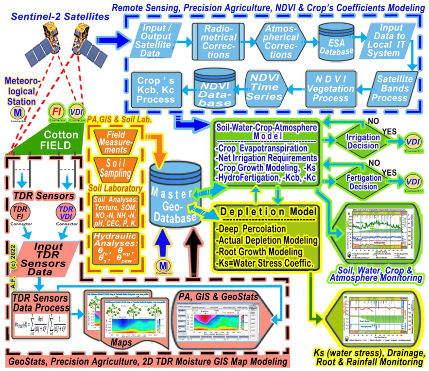
2.1. Experimental Plot Design, Irrigation and Fertilization Treatments, Soil Sampling, and Laboratory Soil and Hydraulic Analysis

For the experiment, an area of 1.79 ha was used from a field of 2.13 ha. The 1.79 ha field that was used had a factorial split plot design, with the main factor being the irrigation treatments: (a) IR1 = VDI or variable deficit irrigation (stage-based deficit irrigation [S-bDI] and fixed partial root-zone variable irrigation [FPRI]); (b) IR2 = common farmers’ irrigation practices [FI] under 2 levels of water deficit each. The levels of IR1 (variable deficit irrigation) were (a.1) IR1-VDI-1 (water deficit 55–77%) and (a.2) IR1-VDI-2 (water deficit 45–77%). The 2 levels of IR2 (farmers’ irrigation) were (b.1) IR2-FI-1 (water deficit 90–95%) and (b.2) IR2-FI-2 (water deficit 95–110%). The sub-factor was three fertilization treatments: Ft1:N-P-K = 124.40–20.16–38.35 Kg·ha⁻¹, Ft2:N-P-K = 150.90–26.71–50.80 Kg·ha⁻¹, and Ft3:N-P-K = 102.30–17.55–33.37 Kg·ha⁻¹. The size of each experimental plot unit was 0.0747 ha, each containing 16955 plants. The layout and size of the 24 plots were designed that way because it was suitable and easier for the correct application of the drip irrigation system, as well as the water cleaning and fertigation system, with an intention to achieve a high distribution uniformity of irrigation water and an easy harvest.

The flow chart of the conceptual design of the soil and hydraulic analyses; field measurements; TDR sensor monitoring; satellite monitoring; 2D TDR soil moisture GIS map modeling; and SWCA, depletion, and NDVI models developed in the present study are depicted in Figure 1.

There are four major model inputs:

(a)

Blue dash line input section, named “Remote sensing, Precision Agriculture, NDVI & Crop’s coefficients Modeling”;

(b)

Brown dash line input section, named “PA, GIS & Soil Lab.”;

(c)

Black dash line input section, named “Geostats, Precision Agriculture, 2D-TDR Soil Moisture GIS Map Modeling”;

(d)

The “M” input section, named “Meteorological Station”, with various sensors providing the local climatic data.

There is a master geodatabase data storage section, named “Master Geodatabase”.

There are two model processing sections named:

(a)

The soil–water–crop–atmosphere model;

(b)

The depletion model.

The models used are further explained later in the manuscript.

A GPS receiver was used to identify the locations of soil samples that were collected at a depth of 0–30 cm, and then analyzed at the applied soil science laboratory of the department.

The soil samples were airdried and passed through a 2 mm mesh to determine the soil texture [(clay content (Cl), silt (Si) content, and sand (Sa) content] via the Bouyoucos hydrometer method [38]. The soil’s pH was measured in a 1:2 soil/water extract, with a glass electrode and a pH meter. Soil organic matter was analyzed via chemical oxidation with 1 mol·L⁻¹ of K₂Cr₂O₇ and titration of the remaining reagent with 0.5 mol·L⁻¹ of FeSO₄ [38].

The cation exchange capacity (CEC) was analyzed (i) by saturating cation exchange sites with Na via the “equilibration” of soil with pH 8.2, as well as 60% ethanol solution of 0.4N NaOAc and 0.1N NaCI; and (ii) by extraction with 0.5N MgNO₃. The total Na and CI amounts were determined in the extracted solution [38]. The soil’s nitrate and ammonium nitrogen contents were extracted with 0.5 mol L⁻¹ of CaCl₂ and were estimated via distillation in the presence of MgO and Devarda’s alloy, respectively. Available phosphorus P (Olsen method) was extracted with 0.5 mol L⁻¹ of NaHCO₃ and measured by spectroscopy [38]. The potassium exchangeable K forms were extracted with 1 mol L⁻¹ of CH₃COONH₄ and measured with a flame photometer. The field capacity (FC) and wilting point (WP) of the soil samples were measured using the porous ceramic plate method, with 1/3 Atm for FC and 15 Atm for WP [3].

2.2. Farm machines, Irrigation Network, Soil, Fertilization, and Crop Management

The field was ploughed on 20 November 2019 with a 4-furrows reversible mounted plough. A spring-tine cultivator (with 26 spring steel tines, reversible points, and floating wings wheels) was applied at field’s soil on 5 February 2020. This type of row crop cultivation machinery is designed to till the soil between the rows of crop, both aerating the soil and uprooting and killing any weeds. Moreover, the floating wing wheels make a clean, tidy, smooth, and consistent soil seedbed finish for maximum seed germination and plant growth.

Field plots were fertilized with the basic (starter) fertilization, which was applied as a broadcast fertilizer application prior to seedbed preparation. The fertilizer used was a granular N-P-K fertilizer [total nitrogen: 15%, phosphorus pentoxide (P₂O₅): 15%, potassium oxide Κ₂O: 15%], enhanced by a urease inhibitor “Agrotain” and incorporated into 30 cm of topsoil with a disk harrow machine. The application doses of nitrogen (N), phosphorus (P), and potassium (K) for the three fertilization treatments were Ft1:N-P-K = 46.20–20.16–38.35 Kg·ha⁻¹, Ft2:N-P-K = 61.20–26.71–50.80 Kg·ha⁻¹, and in Ft3:N-P-K = 40.20–17.55–33.37 Kg·ha⁻¹, respectively.

The cotton seeds (Gossypium hirsutum var. Armonia) were sown with a precision seed drill at the end of April 2020, with a row spacing of 0.970 m and an in-row spacing of 0.045 m. The cotton cultivar ‘Armonia’ was used because it is suitable for dense planting, good ventilation, light transmission among populations, high adaptability to different soil and climatic conditions, excellent resistance and performance of open cotton bolls after heavy rainfall, early maturity, and high yield. The seed metering disc of the precision seed drill was chosen based on the seed type (cotton seed) and population (spacing) required. Advantages of the precision seed drill include the gentle suction from the vacuum unit, the ability to precisely hold each seed “one by one” into the metering disc holes, and the depth of seeds in the soil bed being controlled by dual gauging wheels. The precision seed drill has an optical seed counter which is extremely accurate, equipped with dual optical sensors that count every seed and then relay the readings back to the control box inside the tractor cab. These optical sensors are enclosed under the drill’s metering unit and above the seed tube in order to prevent dust and soil particles being counted as seed, potentially causing inaccurate seed count readings.

The irrigation network consisted of a head unit with a hydrocyclone, a screen filter, a hydrofertigation system, various accessories, a main water delivery pipe and primary and secondary pipes (aluminum: Φ = 110 mm/16.21 bar), and drip laterals (polyethylene: pipes Φ = 20 mm/6.08 bar) with inline pressure-compensated emitters. Before being used in the field experiments, the emitters were tested in the laboratory, as well as in the field, to ensure proper function. Emitters had a discharge rate of 3.8 L·h⁻¹ at 253.31 kPa pressure after testing, according to I.S.O. standards [39]. The inline pressure-compensated emitters had a 1 m distance between each other and the drip laterals were positioned in the middle (48.5 cm) of every other row (194 cm between drip laterals). The fixed partial root-zone variable irrigation [FPRI] had wet soil between the first and second cotton row, dry soil between the second and third row, wet soil between the third and fourth cotton row, and so on. The irrigation technique controlled the soil moisture after the sowing, and the favorable environmental conditions (proper air, and soil temperature) over the following days, helped the seedlings emerge on 5 May with a density of 226,804 plants·ha⁻¹.

Three additional doses of fertilizer (hydrofertigation) were applied using the drip irrigation system at 65, 86, and 93 days after sowing (DAS) by applying a water-soluble urea N-P-K (46–0–0) fertilizer (CO(NH₂)₂) [nitrogen 46%]. The first two additional doses were applied in 65 and 86 DAS during late Ldev (crop development growth stage or flowering [18]). The total amounts of the two N-P-K application doses for the three fertilization treatments during the late Ldev growth stage were Ft1:N-P-K = 55.20–0.00–0.00 Kg·ha⁻¹, Ft2:N-P-K = 69.00–0.00–0.00 Kg·ha⁻¹, and Ft3:N-P-K = 41.40–0.00–0.00 Kg·ha⁻¹. The third dose was applied in 93 DAS during early Lmid (the mid-season growth stage [18] or bolling) with N-P-K application doses of Ft1:N-P-K = 23.00–0.00–0.00 Kg·ha⁻¹, Ft2:N-P-K = 20.70–0.00–0.00 Kg·ha⁻¹, and Ft3:N-P-K = 20.70–0.00–0.00 Kg·ha⁻¹. The season’s total amount of N-P-K fertilizer applied as a basic (starter) fertilization plus hydrofertigation had a total application dose of nitrogen (N), phosphorus (P), and potassium (K) for the three fertilization treatments (Ft1:N-P-K = 124.40–20.16–38.35 Kg·ha⁻¹, Ft2:N-P-K = 150.90–26.71–50.80 Kg·ha⁻¹, and Ft3:N-P-K = 102.30–17.55–33.37 Kg·ha⁻¹).

Finally, cotton plots were harvested on the 10 ten days (1st pick harvest) and the last ten 10 days (2nd pick harvest) of October.

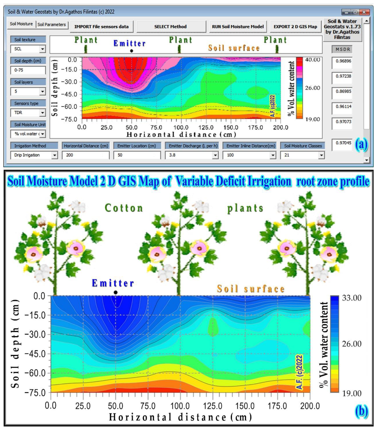
2.3. Soil Moisture Measurements, Digital 2D GIS Moisture Maps Utilizing GIS, Precision Agriculture, Geostatistics, and Average Soil Water Content of Soil Layers

Soil moisture measurements were performed daily by applying the time domain reflectometry (TDR) method, which is a non-radioactive method based on the direct measurement of the dielectric constant of soil and its conversion to water volume content [22,28,40,41,42,43], which has proven to be quick and reliable, irrespective of soil type, except in extreme cases of soils [22,40,41,42,43]. The TDR method was used because it gives accurate results within an error limit of ±1% [3,14,20,21,22,28,36]. A TDR instrument and probes with 5 sensors each were used [3,14,20,21,22,28,36,40,43], placed at 0–15, 15–30, 30–45, 45–60, and 60–75 cm depths for measuring the volumetric water content (θvi, …, θvn) (I = 1, 2, …, n and n = 5) of the cotton’s root-zone in n soil layers. Data measurements were imported daily in a geodatabase, utilizing precision agriculture and geostatistics [3,14,28,36,44] in order to model and produce soil moisture 2D GIS maps of the cotton’s root-zone profile.

Moreover, in order to incorporate the daily average ground-based volumetric water content θv_(TDR) into the SWCA model, the daily average θv_(TDR) was estimated by interpolating the daily soil moisture observations of the different depths (0–15, 15–30, 30–45, 45–60, and 60–75 cm) belonging to the different soil layers of the cotton’s root-zone using Equation (1):

$$\theta v_{\left(TDR\right)}\left(d\right)={\displaystyle \sum }_{i=1}^n\frac{\theta vi}{{\left(dij+s\right)}^p} /{\displaystyle \sum }_{i=1}^n\frac{1}{{\left(dij+s\right)}^p}$$

(1)

where

θv_(TDR)(d) = the estimated average soil water content value for location j;

θvi = the measured sample TDR sensor’s soil moisture value at soil depth point i in the soil layer i;

dij = the distance between θv_(TDR)(d) and θvi;

s = a smoothing factor;

p = a weighting power;

n = the total number of soil layers in the root-zone.

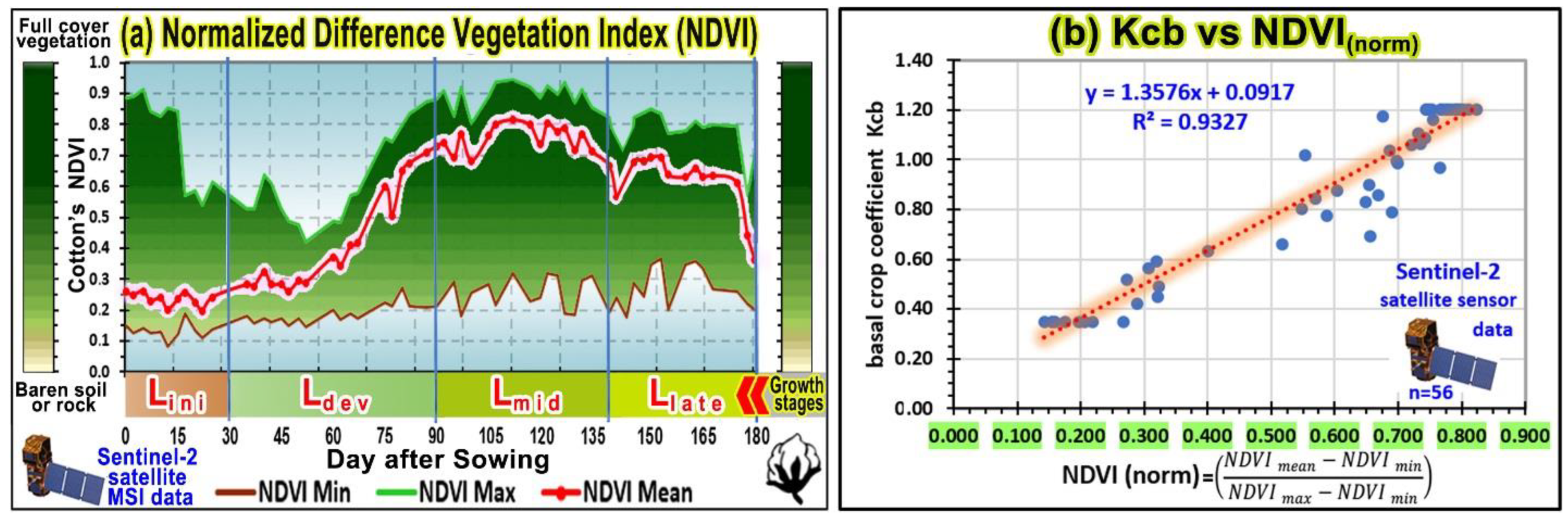
2.4. Remote-Sensing (Satellite) Data and Crop’s NDVI

The Copernicus Sentinel-2 satellite’s mission supports the monitoring of Earth’s surface changes and comprises a constellation of two polar-orbiting satellites placed in the same sun-synchronous orbit, phased at 180° to each other. It has a wide swath width (290 km) and a high temporal resolution (revisit frequency to a particular earth’s location), which is 10 days at the equator with 1 satellite and 5 days with 2 satellites under cloud-free conditions, resulting in 2–3 days at mid-latitudes. A total of 56 Sentinel-2 (A and B) cloud-free images from April 2020 to October 2020 were downloaded from ESA’s Copernicus Open Access Hub [45]. The Sentinel-2 satellite carries onboard sensors as payload multi-spectral instruments (MSIs) which provide information at 13 spectral bands (443–2190 nm) with three types of spatial resolution (10, 20, or 60 m pixel sizes). The 13 spectral bands of the Sentinel-2 MSI satellite range from visible (VNIR) and near-infrared (NIR) to the short-wave infrared (SWIR), as shown below:

(a)

4 × 10 m bands: three classical RGB bands (blue (~493 nm), green (560 nm), and red (~665 nm)) and a near-infrared (~833 nm) band;

(b)

6 × 20 m bands: 4 narrow bands in the VNIR vegetation red edge spectral domain (~704 nm, ~740 nm, ~783 nm, and ~865 nm) and 2 wider SWIR bands (~1610 nm and ~2190 nm);

(c)

3 × 60 m bands mainly focused towards cloud screening and atmospheric correction (~443 nm for aerosols and ~945 nm for water vapor) and cirrus detection (~1374 nm).

In the present study, level 2A reflectance products (radiometrically and atmospherically corrected) from the bottom of atmosphere (BOA), provided by ESA, were used.

All satellite images were resampled at a 10 m pixel size using the sentinel application platform (SNAP)-ESA v.8.0.0 [46] based on free open-source software. After the data extraction of pixels for the studied experimental site (cotton field), the time series were constructed for the normalized difference vegetation index (NDVI). The NDVI vegetation index [3,14,28,36,47] was derived from the data of the 56 downloaded remote-sensing images using near-infrared and red bands. This vegetation index utilizes the reflectance of the canopy in the near-infrared (NIR) and red (R) bands of the spectrum [3,28,36,47].

The NDVI vegetation index was calculated every week one or two times (depending on the availability of cloud free satellite images) using remote-sensing (RS) data (Sentinel-2 satellites sensor data) for studying spatial crop development and crop coefficients.

The Sentinel-2 satellites band B4[RED] = (~665 nm) and band B8[NIR] = (~842 nm) were used. The NDVI vegetation index [3,14,28,36,47] was computed by Equation (2):

$$NDVI=\frac{\rho NI{R}_{\left(842\right)}-\rho RE{D}_{\left(665\right)}}{\rho NI{R}_{\left(842\right)}+\rho RE{D}_{\left(665\right)}}$$

(2)

where

ρNIR(₈₄₂) = the near-infrared (NIR) band (reflectance at wavelength 842 nm), and

ρRED(₆₆₅) = the red band (reflectance at wavelength 665 nm) of the Sentinel-2 satellite sensors used for calculation. The wavelengths 842 nm and 665 nm denote the center wavelength of the corresponding Sentinel-2 bands.

2.5. Climatic Data Sensors’ Measurements; Net Irrigation Requirements; Reference, Crop, and Actual Evapotranspiration; the Soil–Water–Crop–Atmosphere (SWCA) Model; the Soil Moisture Depletion Model; and the Water Stress Coefficient Ks-Weighted Average

Daily climatic data were obtained from sensor measurements of a weather station nearby to the experimental field. The measured parameters (temperature, relative humidity, atmospheric pressure, wind speed, wind direction, rainfall, and solar radiation) and the technical characteristics of the Wireless Vantage Pro2 Plus weather station [48] used in the present study are shown in

Table 1. The measured parameters and the technical characteristics of the weather station.

Parameter	Sensor Type	Range	Resolution	Accuracy
Temperature	Electronic PN junction silicon diode	−40 to + 65 °C	0.1 °C, −23.3 to +37.8 °C 0.2 °C otherwise	0.3 °C, +15.6 to +37.8 °C 1.7 °C, −40 to +15.6 °C 1.1 °C, +37.8 to +65 °C
Relative humidity	Electronic film capacitor element	0–100%	1%	3%, 0–90% 4%, 90–100%
Atmospheric pressure	Electronic	540–1100 hPa	0.1 hPa	±1.0 hPa
Wind speed	Wind cups with magnetic switch	1–67 m/s, 3–241 km/h (large wind cups) 1.5–79 m/s, 5–282 km/h (small wind cups)	0.5 m/s, 1 km/h	Max (5%, 3 km/h, 1 m/s) (large wind cups) max (5%, 5 km/h, 1.5 m/s) (small wind cups)
Wind Direction	Wind vane with potentiometer	0–360°	1°	3°
Rainfall	Tipping bucket	(0–100 mm/h)	0.2 mm	Max (3%, 0.2 mm), for rain rates up to 50 mm/h max (3%, 0.25 mm), otherwise
Solar radiation	Silicon photodiode with diffuser (400–1100 nm)	0–1800 W/m2	1 W/m2	5%

.

The net irrigation requirement (NIR) was calculated using a daily soil–water–crop–atmosphere (SWCA) balance model (Equation (3)) [3,14,28,36]:

NIR = ETc − Pe − GW − Δθv_(TDR)

(3)

where

NIR = the net irrigation requirement (mm);

ETc = evapotranspiration (mm);

Pe = effective rainfall (mm);

GW = groundwater contribution from the water table (mm);

Δθv_(TDR) is the change in TDR sensors measuring the soil–water content θv_(TDR) (mm).

The effective rainfall for the experimental site conditions was calculated according to USDA-SCS (1970) [49]. The reference evapotranspiration ETo was computed based on the F.A.O. The Penman–Monteith method [3,14,18,28,36] is shown in Equation (4).

$$ETo=\frac{0.408\mathsf{\Delta }\left(Rn- G\right)+\mathsf{\gamma }\frac{900}{T+273}{u}_2\left(e_s-e_a\right)}{\mathsf{\Delta }+ \mathsf{\gamma }\left(1+0.34u_2\right)}$$

(4)

where

ETo = the reference evapotranspiration (mm day⁻¹), Rn = the net radiation at the crop surface (MJ m⁻² day⁻¹), G = the soil heat flux density (MJ m⁻² day⁻¹), T = the mean daily air temperature at 2 m height (°C), u₂ = the wind speed at 2 m height (m s⁻¹), e_s = the saturation vapor pressure (kPa), e_a = the actual vapor pressure (kPa), (e_s − e_a) = the saturation vapor pressure deficit (kPa), Δ = the slope of the vapor pressure curve at temperature Τ (kPa °C⁻¹), and γ = the psychometric constant (kPa °C⁻¹).

The crop evapotranspiration (ETc) was computed as (Equation (5)):

$$ETc=\left(K_{cb}+K_e\right) ETo$$

(5)

ETc = crop evapotranspiration (mm·day⁻¹), ETo = reference evapotranspiration (mm·day⁻¹), (K_cb + K_e) = the dual crop coefficient (dimensionless), K_cb = the basal crop coefficient (dimensionless), K_e = the soil–water evaporation coefficient (dimensionless).

When the topsoil is wet, following rain or irrigation, K_e is maximal. When the soil surface is dry, K_e is small and even zero when no water remains near the soil surface for evaporation.

The actual crop evapotranspiration (ETa) was computed as (Equation (6)):

$$ETa=\left(K_s K_{cb}+K_e\right) ETo$$

(6)

where

ETa = crop evapotranspiration (mm day⁻¹), ETo = reference evapotranspiration (mm·day⁻¹), K_s = the water stress on the crop transpiration coefficient (dimensionless), K_cb = the basal crop coefficient (dimensionless), K_e = the soil–water evaporation coefficient (dimensionless).

The water stress on the crop transpiration coefficient (K_s) has values ranging from 0 to 1, and refers to the condition of soil moisture and other factors, such as the salinity and the prevailing weather conditions [3,18,28,36]. The value of K_s can be influenced by inhibiting environmental factors such as water stress (K_{s_water}) or salinity stress (K_{s_salinity}). The K_s coefficient value of 1 indicates no water stress to plants, while K_s < 1 indicates water stress.

The basal crop coefficient (K_cb) varies depending on the type and growth stages of a given crop (in our case cotton crop). The soil–water evaporation coefficient (K_e) varies depending on the soil surface for evaporation.

The crop evapotranspiration (ETc) and actual evapotranspiration (ETa) were computed using crop coefficients obtained from the remote-sensing NDVI vegetation index [3,14,18,28,36,47]. The NDVI vegetation index was derived from the data of the 56 Sentinel-2 Satellite downloaded remote-sensing images.

This vegetation index utilizes reflectance of the canopy in the near-infrared (NIR) and red (R) bands of the spectrum [3,28,36,47]. The NDVI vegetation index was calculated once or twice every week using remote-sensing (RS) data (Sentinel-2 satellite MSI sensor data) for studying the spatial crop development and crop coefficients.

The root-zone depletion of the available soil moisture was estimated using a daily available soil moisture depletion (ASMD) model (Equation (7)) [3,14,18]:

$$Dr{,}_{\left(i\right)}=Dr{,}_{\left(i-1\right)\left[TDR\right]}–{\left(P-RO\right)}_{\left(i\right)}–I_{\left(i\right)}–C{R}_{\left(i\right)}+ET{c}_{\left(i\right)}+D{P}_{\left(i\right)}$$

(7)

where

Dr,_(i) = root-zone depletion at the end of day I [mm], Dr,_(i−1)[TDR] = root-zone soil–water content measured by TDR sensors at the end of the previous day i − 1 [mm], P_(i) = precipitation on day i [mm], RO_(i) = runoff from the soil surface on day i [mm],I_(i) = net irrigation depth on day i that infiltrates the soil [mm], CR(i) = capillary rise from the groundwater table on day i [mm], ETc_(i) = crop evapotranspiration on day i [mm], DP_(i) = water loss out of the root-zone by deep percolation on day i [mm].

Each stage’s water stress coefficient Ks-weighted average was calculated as (Equation (8)):

$$K{s}_{\mathit{weighted}\_ave}=\left(K{s}_{ave}-\left(\frac{\left(K{s}_{ave} StgDaysK{s}_{<1}\right)}{{\mathrm{StgDur}}_{days}}\right)\left(NumStg\frac{{\mathrm{StgDur}}_{days}}{SumDAS}\right)\right)$$

(8)

where

Ks_{weighted_αve} = stage’s water stress coefficient Ks-weighted average (dimensionless) [–],

Ks_αve = stage’s average Ks (dimensionless) [–], StgDaysKs_<1 = stage’s number of days with water stress coefficient Ks < 1 [days], StgDur_days = stage’s duration in days [days], NumStg = number of crop’s growth stages [–], SumDAS = sum of days after sowing of all growth stages (total days of season) [days}.

2.6. Nitrogen Partial Factor Productivity, Nitrogen–Phosphorus–Potassium Fertilizer Partial Factor Productivity, and Water Use Efficiency (WUE)

The nitrogen partial factor productivity (N_PFP) [50,51] was determined as (Equation (9)):

$$\mathit{N\_PFP}=\raisebox{1ex}{$ Y$}\!\left/ \!\raisebox{-1ex}{$N_t$}\right.$$

(9)

where

Y = the cotton yield of each plot [Kg·ha⁻¹], N_t = the total application of nitrogen fertilizer applied to the crop of each plot [Kg·ha⁻¹].

The nitrogen–phosphorus–potassium fertilizer partial factor productivity (NPK_PFP) was determined as (Equation (10)):

$$\mathit{NPK\_PFP}=Y /{\displaystyle \sum }_{i=1}^n{N}_t,P_t,K_t$$

(10)

where

Y = the cotton yield of each plot [Kg·ha⁻¹],

N_t = the total application of nitrogen fertilizer applied to each plot [Kg·ha⁻¹], P_t = the total application of phosphorus fertilizer applied to each plot [Kg·ha⁻¹], K_t = the total application of potassium fertilizer applied to each plot [Kg·ha⁻¹], n = the total number of applied nutrients to the crop.

The water use efficiency (WUE) of each plot was determined as (Equation (11)):

$$WUE=\raisebox{1ex}{$ Y$}\!\left/ \!\raisebox{-1ex}{$\left(I+Pe\right)$}\right.$$

(11)

where

Y = the cotton yield of each plot [Kg·ha⁻¹], I = the net irrigation volume applied to each plot [mm], Pe = the effective rainfall [mm].

2.7. Field Measurements of Cotton Plant Height, Plant Stem, Boll Weight, and Above-Ground Biomass Dry Matter

At the end of each cotton stage (Lini (the seedling stage), Ldev (the flowering stage), Lmid (the bolling stage), and Llate (the maturity stage)), four representative cotton plants from each experimental plot were sampled destructively, and flowers and fruits (when present) were counted. The definitions of cotton’s phenological stages in the present study are taken from Allen et al. (1998) [18] and Munger et al. (1998) [52]. Moreover, the date the plants entered each phenological stage was recorded for all plots. The measurements of the cotton’s plant height were performed using a tape measure with an accuracy of 1 mm. The measurements of cotton’s plant stem were performed using a digital micrometer with an accuracy of 0.1 mm.

The measurements of the cotton boll (when present) weight were taken with a digital weighing scale with an accuracy of 0.01 g.

The plant sample parts (stem, leaves, flowers, and fruits when present) were dried in a thermo-ventilated oven at 65 °C until it reached a constant weight in order to measure the above-ground biomass dry matter weight (DW). The weight measurements of the cotton’s dried plant parts (above-ground biomass dry matter) were taken with a digital weighing scale with an accuracy of 0.01 g as g DW plant ⁻¹.

2.8. Statistical Data Analysis

Data analysis and two-way ANOVA statistical analysis (p = 0.05) were performed using the IBM SPSS v.26 [3,28,36,53,54,55] statistical software package. The results represent the means of the samples and measurements of all measured and derived data groups. A mean separation was made using the LSD_0.05 statistical test as the test criterion when significant differences (p = 0.05) between treatments were found [3,54].

The zero hypothesis (H0) for the main factor irrigation treatments: (a) IR1 = VDI or variable deficit irrigation (stage-based deficit irrigation [S-bDI] and fixed partial root-zone variable irrigation [FPRI]); (b) IR2 = common farmers’ irrigation practices]) under 2 levels of water deficit each as (a.1) IR1-VDI-1 (water deficit 55–77%), (a.2) IR1-VDI-2 (water deficit 45–77%), (b.1) IR2-FI-1 (water deficit 90–95%), and (b.2) IR2-FI-2 (water deficit 95–110%), for the sub-factor [Ft1:N-P-K = 124.40–20.16–38.35 Kg·ha⁻¹, Ft2:N-P-K = 150.90–26.71–50.80 Kg·ha⁻¹, and Ft3:N-P-K = 102.30–17.55–33.37 Kg·ha⁻¹] and for irrigation and fertilization treatment interaction effects on the cotton yield, nitrogen fertilizer partial factor productivity (N_PFP), N-P-K fertilizer PFP, water use efficiency, plant height, plant stem, boll weight, and above-ground biomass dry matter (H0ir, H0ft, and H0irxft, respectively), as seen below:

H0ir = irrigation treatments ((a) IR1 = VDI or variable deficit irrigation (stage-based deficit irrigation and fixed partial root-zone variable irrigation) under water deficit levels (wdl) (a.1) IR1-VDI-1 (wdl 55–77%) and (a.2) IR1-VDI-2 (wdl 45–77%)) and ((b) IR2 = common farmers’ irrigation practices under water deficit levels (b.1) IR2-FI-1 (wdl 90–95%) and (b.2) IR2-FI-2 (wdl 95–110%)) have no significant effect on the cotton yield, nitrogen fertilizer partial factor productivity (N_PFP), N-P-K fertilizer PFP, WUE, plant height, plant stem, boll weight, and above-ground biomass dry matter.

H0ft = fertilization treatments [Ft1:N-P-K = 124.40–20.16–38.35 Kg·ha⁻¹, Ft2:N-P-K = 150.90–26.71–50.80 Kg·ha⁻¹, and Ft3:N-P-K = 102.30–17.55–33.37 Kg·ha⁻¹] have no significant effect on the cotton yield, nitrogen fertilizer partial factor productivity (N_PFP), N-P-K fertilizer PFP, WUE, plant height, plant stem, boll weight, and above-ground biomass dry matter.

H0irxft = irrigation and fertilization treatments interaction have no significant effect on the cotton yield, nitrogen fertilizer partial factor productivity (N_PFP), N-P-K fertilizer PFP, WUE, plant height, plant stem, boll weight, and above-ground biomass dry matter.

2.9. Geostatistical Analysis and Modeling, Spatial Interpolation Methodology, and Model Validation Process

For the various experimental farm field GIS variable maps, spatial interpolation was used with the geostatistical models of ordinary and universal kriging, which are used to estimate an unknown value, given the observed values at sampled plots [3,9,14,20,22,28,36,56,57,58,59,60]. The kriging method is based on the assumptions that the variable’s attribution values (cotton yield, nitrogen fertilizer PF productivity, N-P-K fertilizer PF productivity, WUE, and cotton boll weight) at the unsampled field sites are a weighted average of values at sampled sites of the experimental farm field.

Using the parameters found from measurements (which were digitally mapped in a GIS geodatabase environment), we delineated the cotton yield, nitrogen fertilizer PF productivity, N-P-K fertilizer PF productivity, water use efficiency (WUE), and cotton boll weight field GIS maps with the help of spatial analysis and modeling.

In addition, the evaluation or validation of the geostatistical models results require statistical analysis of residual errors, the difference between predicted and observed values, and prediction characterization between over- and under-estimates. To that end, we used the statistical parameters described by other studies [3,9,14,20,22,28,36,57,58,59,60,61], such as the equations for the mean prediction error (MPE), the root-mean-square error (RMSE), the mean standardized prediction error (MSPE) as a measure of unbiased predictions [3,62,63], and the root-mean-square standardized error (RMSSE) as a measure of correctly assessing the variability of prediction [3,63,64].

The MSPE and RMSSE were used to assess the unbiasedness and estimation of uncertainty, respectively. The MPE and MSPE values should approach zero for an optimal prediction, the RMSSE should approach one, and a lower RMSE value should improve the RMSE for an optimal prediction.

3. Results and Discussion

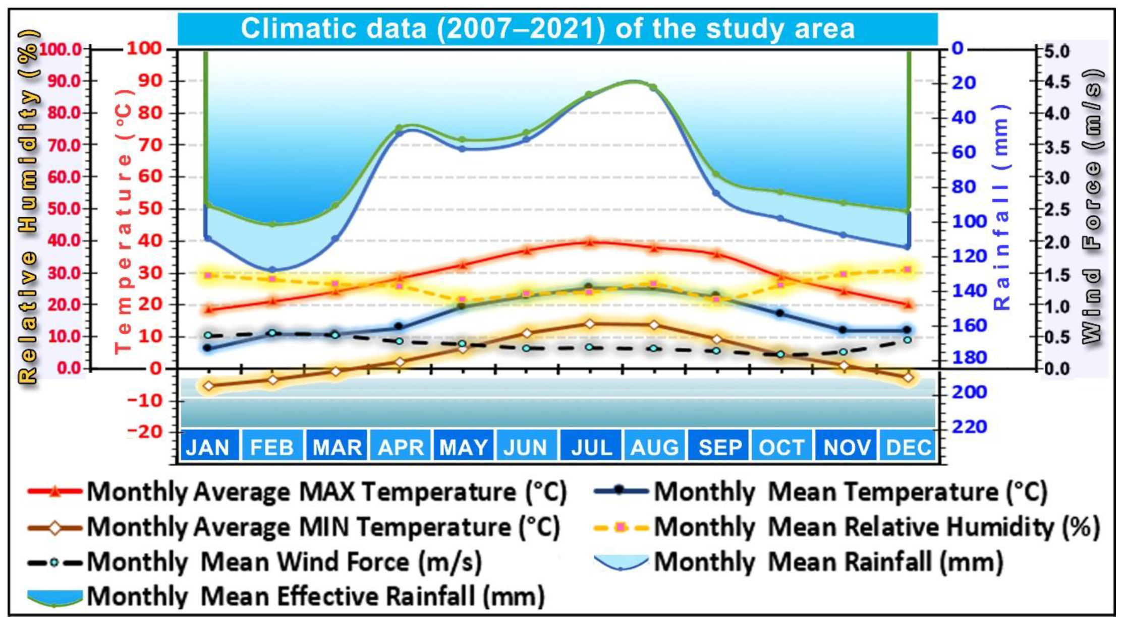
3.1. Study Area of the Farm Field, Climatic Data Analysis for The Recent 15 Years (2007–2021), and Results and Discussion of Soil and Hydraulic Analysis of the Field’s Soil

The present experiment was conducted in a farm field located at a flat study area called the “Viotoia” valley, of the “Viotoia” prefecture of the “Sterea” Greek region. The various mean monthly climatic data for the recent 15 years (2007–2021) of the study area are depicted in Figure 2.

The study area is characterized by a typical Mediterranean climate [3,9] with a cold winter, a hot summer with frequently occurring high air temperatures, and low precipitation amounts in spring and summer.

The area has an average annual rainfall of 960 mm, an average air temperature of 16.32 °C, an average maximum air temperature of 28.93 °C, an average minimum air temperature of 4.14 °C, and a frost-free period lasting 224 days. In the recent 15 year period, the maximum air temperature was 39.39 °C and the minimum air temperature was −5.26 °C.

A first reading of the presented climatic data values indicates that the air temperatures (mean, maximum, and minimum), relative humidity, and wind force show acceptable values that permit the cotton’s proper growth.

On the contrary, the precipitation amount and its distribution through time on the four crop growth stages (April to October) do not quite cover crop water needs, in light of rainfed cultivation on all stages for the cotton’s proper growth, so irrigation is essential in order to obtain a good yield. In fact, the total rain fell during the cotton-growing season (April to October) was 410.70 mm while the cotton’s crop evapotranspiration was 766.90 mm (calculated with the Penman–Monteith method [3,18,28,36,65]).

The results of the laboratory soil and hydraulic analysis revealed that the field’s soil was suitable for cotton growth [3,18,38,49], and was characterized as sandy clay loam (SCL) [3,18,49].

The soil parameters that are required to determine the daily soil evaporation coefficient Ke include the soil moisture at field capacity (θfc) and wilting point (θwp), the readily evaporable water REW, and the depth Ze of the surface soil layer that is subject to drying by way of evaporation. Soil’s hydraulic analysis results found a θfc = 0.325 m³ m⁻³, a θwp = 0.194 m³ m⁻³, a REW = 9.77 mm, and a plant available water PAW = 0.131 cm cm⁻¹ (±0.03). The bulk specific gravity of the soil was 1.42 g cm⁻³ (±0.03).

Soil texture, which refers to the proportions of sand, silt, and clay, influences almost every aspect of soil management and soil use for cultivation. We observe that for the experimental field soil texture (clay = 48%, loam = 26% and sand = 26%), the values of θfc and θwp found by soil hydraulic analysis are in the ranges given by Allen et al. (1998) [18]. Moreover, Allen et al. (1998) [18] suggests that the value of the depth of soil surface evaporation layer Ze (m) is between 0.10 and 0.15 m. In the present study, the value of Ze = 0.1 m was used in the calculations.

Soil organic matter (SOM) was 1.83% (±0.18), which is considered as an adequate SOM level [3,21,58]. SOM is widely regarded as a vital component of soil’s fertility because of its major role in physical, chemical, and biological processes which take place through the cultivation season and supply the plants with various nutrients. Furthermore, SOM helps to maintain soil structure and soil moisture-holding capacity, enhances the ability of the soil to hold nutrients, and improves drainage.

The pH at (1:2) the soil–water extract was 8.03 (±0.23) and was classified as alkaline. The soil’s pH is a measure of the hydrogen ion concentration and the optimum value for cotton is 6.5 [66]. The value for cotton is considered to reach a tolerable level [3,36].

The N-NO₃ was 9.85 mg kg⁻¹ (±2.27) [a marginal level] and the N-NH₄ was 3.19 mg kg⁻¹ (±1.07) [a low level].

Plants can easily uptake the above two forms of soil nitrogen (N): nitrate (N-NO₃⁻) and ammonium (N-NH₄⁺). The N-NH₄⁺ form is held in the soil by negatively charged soil clays or colloids. The negatively charged N-NO₃⁻ form is repelled by soil particles and is subject to movement with water in the soil profile. In order to achieve an economic yield, cotton plants must be fertilized with the right amount of nitrogen in all phases of growth and fruit development [3]. Excessive nitrogen supply delays maturity, causes rank growth, intensifies insect infestations, encourages diseases, and increases the risk of boll rot and reduced lint quality. A nitrogen deficiency will cause small stalks, pale green leaves, small bolls, fruit shed, and low yields [67].

It is essential and environmentally friendly to apply nitrogen according to the crop’s needs in order to reduce residual soil nitrogen at the end of the cultivation season and leave little available nitrogen for losses. Thus, it is important to study the nitrogen fertilizer amount that gives an economic yield without deficiency’s negative side-effects. Thus, we choose three fertilization treatments under VDI and farmers’ common irrigation, and statistically investigated the three yields and the three nitrogen PFPs.

The phosphorus P-Olsen was 18.72 mg kg⁻¹ (±2.27) [a sufficient level], and the potassium K-exchangeable reached high concentration levels (512 mg kg⁻¹ (±21.37)).

Phosphorus has low mobility in the soil, and leaching is not considered a problem [3,66]. Instead, mobility to the roots is the prime limitation to uptake methods. Because of the low mobility of phosphorus, root interception is the prime method of uptake, regardless of the soil pH. Cotton roots are aided in their interception of soil phosphorus by mycorrhizal fungi [66].

Potassium mobility in soils is in the intermediate level between nitrogen and phosphorus, but is not easily leached because it has a positive charge (K⁺), which causes it to be attracted to negatively charged soil colloids [3,66]. The cotton’s peak needs potassium during the boll filling; in order to be available at this time, potassium must be in solution where late-season roots are inactive.

Finally, the cation exchange capacity of the soil was 19.92 cmol kg⁻¹ (±1.07), which is a sufficient level, indicating the good soil fertility.

3.2. Results and Discussion of the 2D Moisture Model and GIS Maps of Cotton’s Root-Zone Soil Profile Utilizing GIS, Precision Agriculture, and Geostatistics

An example of the produced digital soil moisture model 2D GIS maps, using “Soil & Water Geostats v.1.73”, software for cotton’s root-zone soil profile of a farmers’ drip irrigation plot is depicted in Figure 3a and the VDI drip irrigation plot is depicted in Figure 3b (with annotated cotton plants).

Soil moisture is a major factor affecting crops’ enhanced growth and production [3,14,22,28,36].

The TDR sensor measurements (average of the soil moisture content measurements at five different soil depths [0–15 cm, 15–30 cm, 30–45 cm, 45–60 cm, and 60–75 cm]) were used in order to monitor the daily soil moisture ${\theta }_{V\left(TDR\right)}$ and the depletion of available soil moisture (ASMD) [3,14,20,21,22,28,36] that was calculated and evaluated in relation to each VDI and the farmers’ drip irrigation treatment.

The TDR measurement datasets (data on five different soil depths) of soil moisture were imported in a digital geodatabase and used to model and produce digital soil moisture two-dimensional (2D) maps of the cotton’s root-zone soil profile of the plots by utilizing precision agriculture and geostatistics [3,14,20,21,22,28,36].

Spatial analysis revealed a typical moisture distribution for sandy clay loam (SCL) soil. The soil moisture model 2D GIS maps (Figure 2a,b) of the cotton’s root-zone modeled from TDR sensors’ data measurements shed light and offer valuable knowledge on the soil moisture exact status in the cotton’s root-zone soil profile through the growth season, helping the right irrigation decisions to be made for the VDI irrigation treatment plots. The same concept with similar results was used in previous case studies [3,14,22,28,36].

It is worth noting that farmers with no access to the digital soil moisture GIS model 2D maps of the cotton’s root-zone soil profile monitoring or to the SWCA and the depletion model data results simply used their experience and their own “eyes” for crop monitoring, but they could not “see” the cotton’s root-zone moisture profile through soil’s surface, so their irrigation common practice decisions did not always allow correct irrigation management.

3.3. Results of Sentinel-2 Satellite MSI Sensor Data Analysis and NDVI Vegetation Index of the Cotton’s Farm Field

In order to achieve accurate irrigation scheduling, it is fundamental to determine the daily crop evapotranspiration (ETc) and the actual crop evapotranspiration (ETα) during the growing period. A practical method that is usually applied for estimating ETc is the crop coefficient (Kc) approach [18], in which an experimentally developed dimensionless Kc is multiplied by reference evapotranspiration (traditionally grass or alfalfa) in order to compute ETc (see above Equation (5)). Moreover, in FAO-56 [18], the dual crop coefficient Kcb procedures are used to compute more precise estimates of daily ETc and ETα for days following irrigation or rain. For the FAO-56 dual crop coefficient approach, the single Kc is separated into two coefficients: a basal crop coefficient (Kcb) for primarily crop transpiration and a wet soil evaporation coefficient (Ke) to quantify the individual contributions for the two components of ETc. The dual procedures also include a water stress coefficient (Ks) to quantify the effects of soil water stress on ETc.

Because the Kcb curve functions described in FAO-56 [18], and generally those used with most state-of-the-art irrigation scheduling programs, are time-based, they lack the flexibility required to capture a typical crop development and water use patterns caused by weather anomalies [65].

Remote-sensing methods and the derived vegetation indexes offer a good solution for overcoming many of the shortcomings of the conventional crop coefficient in ETc and ETα calculation by providing real-time feedback satellite sensors images on daily crop water use, as influenced by the field’s actual crop development spatial patterns, the local prevailing atmospheric conditions of the area, and the field’s spatial variability of soil and hydraulic characteristics.

The NDVI vegetation index [3,14,28,36,47] was calculated once or twice every week (depending on the availability of cloud free satellite images) using remote-sensing (RS) data (Sentinel-2 satellite MSI sensors data) for monitoring spatial crop development patterns and deriving crop coefficients for the SWCA and depletion models. The NDVI vegetation indexes were derived from 56 Sentinel-2 satellite images.

The fluctuation of the NDVI vegetation index for the four cotton growth stages is depicted in Figure 4a. Although several regression equations and time based NDVI vegetation indexes were considered, a simple multiple linear regression function with the NDVI vegetation index for the crop growth spatial patterns capturing in real daily field conditions was selected for modeling the observed basal crop coefficient (K_cb) (Figure 4b). The best derived equation found with an R² = 0.9327 is presented in Equation (12):

$$K_{cb}=1.3576 \left(\frac{NDVI{ }_{mean}-NDVI{ }_{min}}{NDVI{ }_{max}-NDVI{ }_{min}}\right)+0.0917$$

(12)

where

K_cb = the basal crop coefficient (dimensionless), $NDVI{ }_{mean}=$ the mean daily value of field’s MSI-sensed NDVI, $NDVI{ }_{min}=$ the minimum daily value of field’s MSI-sensed NDVI, and $NDVI{ }_{max}$ = the maximum daily value of field’s MSI-sensed NDVI.

The use of Equation (12), derived above, is proposed for cotton plantations in Mediterranean conditions with remote-sensing data images (Sentinel-2 satellite multispectral instrument (MSI) sensors) for basal coefficient calculation in order to obtain a real-time feedback of satellite sensor images on daily crop water use, as influenced by the field’s actual crop development spatial patterns, the local prevailing atmospheric conditions of the area, by the field’s spatial variability of soil and hydraulic characteristics.

The near-infrared (NIR) band (ρNIR(₈₄₂) = reflectance at wavelength 842 nm) and the red band (ρRED(₆₆₅) = reflectance at wavelength 665 nm) of the Sentinel-2 satellite sensors were used for NDVI calculations. The wavelengths 842 nm and 665 nm denote the center wavelength of the corresponding Sentinel-2 bands.

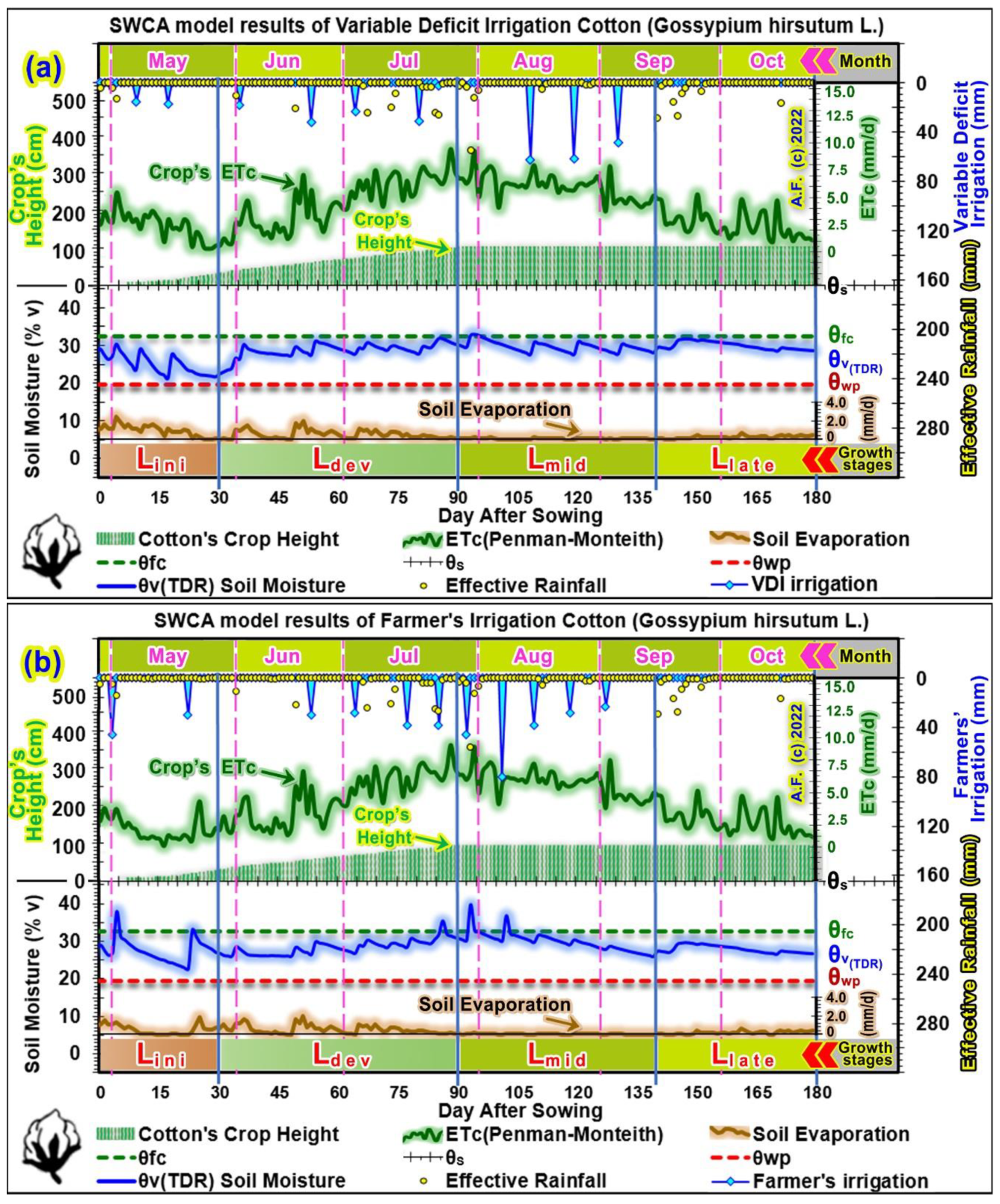
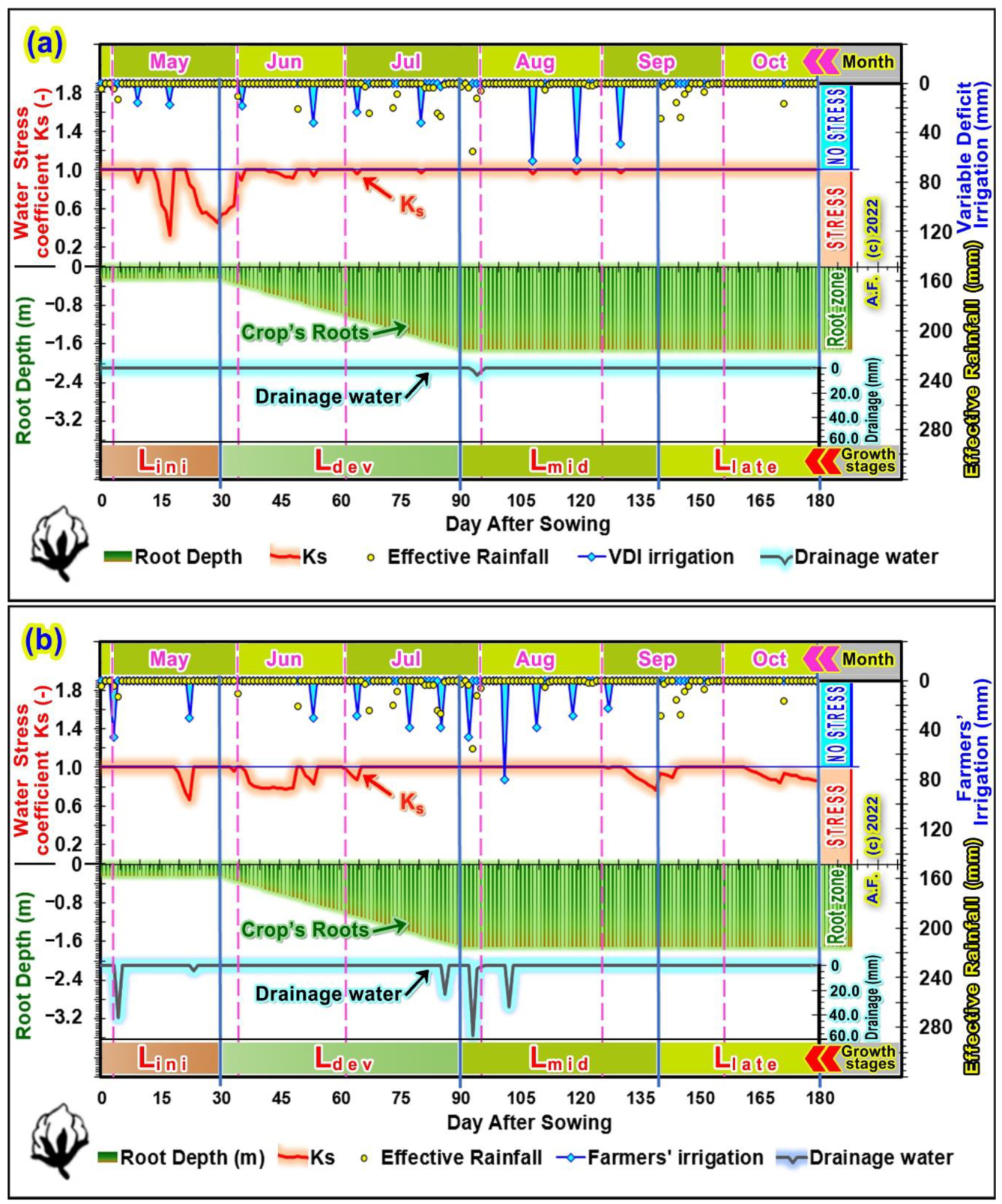
3.4. Results and Discussion of The Variable Deficit Irrigation, Farmers’ Irrigation, Daily Soil–Water–Crop–Atmosphere (SWCA) Model, Water Stress Coefficient Ks, and the Availiable Soil Moisture Depletion Model

In the present study, we define water deficit at six levels, as presented in

Table 2. The water deficit levels depending on soil water level.

Sn	Water Deficit Level	Abbreviation	Soil Water Level	Description
1	Severe water deficit	SevWD	$<50\% \mathrm{of} {\theta }_{fc}$	$\mathrm{soil} \mathrm{water} \mathrm{is} \mathrm{less} \mathrm{than} 50\% \mathrm{of} {\theta }_{fc}$
2	Moderate water deficit	ModWD	$50–60\% \mathrm{of} {\theta }_{fc}$	$\mathrm{soil} \mathrm{water} \mathrm{remains} \mathrm{between} 50 \mathrm{to} 60\% {\theta }_{fc}$
3	Mild water deficit	MildWD	$60.1–75\% \mathrm{of} {\theta }_{fc}$	$\mathrm{soil} \mathrm{water} \mathrm{remains} \mathrm{between} 60.1 \mathrm{to} 75\% {\theta }_{fc}$
4	Light water deficit	LightWD	$75.1–90\% \mathrm{of} {\theta }_{fc}$	$\mathrm{soil} \mathrm{water} \mathrm{remains} \mathrm{between} 75.1 \mathrm{to} 90\% {\theta }_{fc}$
5	No deficit or full irrigation	NoWD	$>90\% \mathrm{of} {\theta }_{fc}$	$\mathrm{soil} \mathrm{water} \mathrm{is} \mathrm{greater} \mathrm{than} 90\% \mathrm{of} {\theta }_{fc}$ during the key plant growth period
6	Over-irrigation	OverIRR	$>100\% \mathrm{of} {\theta }_{fc}$	irrigation water amount may be greater than plant’s water requirements for optimal growth

.

Variable deficit irrigation (VDI) is defined as an irrigation management strategy whereby crops are irrigated with a variable water amount that is usually less than the crop’s full requirement (actual evapotranspiration) for optimal plant growth, in order to reduce the total amount of irrigation water used in the irrigation season, improve the response of plants to water deficit in a positive way, and increase the crop’s water use efficiency.

Figure 5a depicts the results of the daily soil–water balance model [3] with the daily monitoring of soil moisture ${\theta }_{V\left(TDR\right)}$ (measured with TDR instrument and sensors [3,14,20,21,22,28,36]), effective rainfall, VDI irrigation, crop’s evapotranspiration, cotton’s crop height evolution, saturation ${\theta }_S$ (soil moisture content at saturation), field capacity (${\theta }_{fc}$), permanent wilting point (${\theta }_{wp}$), and soil evaporation through the four crop growth stages of treatment for IR1:VDI-2 or variable deficit irrigation (stage-based deficit irrigation [S-bDI] and fixed partial root-zone variable irrigation [FPRI]).

Figure 5b depicts the results of the daily soil–water balance model [3] with the daily monitoring of soil moisture ${\theta }_{V\left(TDR\right)}$ (measured with TDR instrument and sensors [3,14,20,21,22,28,36]), effective rainfall, farmers’ irrigation, crop’s evapotranspiration, cotton’s crop height evolution, saturation ${\theta }_S$, field capacity $({\theta }_{fc})$, permanent wilting point (${\theta }_{wp})$, and soil evaporation through the four crop growth stages of the IR2:FI-2 treatment for farmers’ common irrigation practices.

3.4.1. Results and Discussion of the Lini: Initial Crop Growth Stage or Seedling

The duration of the initial crop growth stage [18] or other seedling [52] was 30 days, which extends from the sowing date to approximately 10% ground cover by plants’ green vegetation. Definitions of cotton’s phenological stages in the present study are taken from Allen et al. (1998) [18] and Munger et al. (1998) [52].

During the initial stage Lini, the SWCA model’s θpini was set to 0.65 (that is MAD = 65%, where MAD = management allowable depletion [3,18,28]) for the cotton’s growth with no water stress. MAD is a term that describes how much of the available soil water can be depleted before it is replaced with irrigation.

As shown in Figure 5a,b and in

Table 3. Crop growth stage parameters and results of the SWCA model and the depletion model.

	Crop Growth Stage of Cotton (Gossypium hirsutum L.)
Parameter	L Ini		L Dev		L Mid		L Late		Total
Stage duration in days	30		60		50		40		180
Irrigation treatment	IR1:VDI	IR2:FI	IR1:VDI	IR2:FI	IR1:VDI	IR2:FI	IR1:VDI	IR2:FI	IR1:VDI	IR2:FI
Water deficit [%]	60–70%	95–110%	45–77%	95–110%	55–75%	95–110%	--*	--*	45–77%	95–110%
ASMD average [%]	56.43	37.69	29.47	31.29	21.92	18.91	19.73	34.76	29.85	29.74
ASMD max [%]	86.10	75.62	77.09	49.21	37.65	49.78	30.95	45.34	86.10	75.62
Ks average [–]	0.845	0.975	0.963	0.946	0.998	0.977	1.000	0.949	0.960	0.960
Ks max [–]	1.000	1.000	1.000	1.000	1.000	1.000	1.000	1.000	1.000	1.000
Ks min [–]	0.319	0.662	0.540	0.772	0.957	0.764	1.000	0.836	0.319	0.662
Ks-weighted average [–]	0.830	0.969	0.941	0.918	0.994	0.964	1.000	0.919	0.918	0.883
Number of days with Ks < 1 (indicates water stress to plants)	13	4	16	21	3	10	0	23	32	58
Percentage of days with Ks < 1 (indicates water stress to plants)	43.33	13.33	26.67	35.00	6.00	20.00	0.00	57.50	17.78	32.22
Irrigation NIR [mm]	33.11	76.08	109.71	134.50	176.55	214.90	0.00	0.00	319.37	425.48
Effective rainfall Pe = P-RO [mm]	27.05	27.05	154.25	154.25	91.84	91.84	115.82	115.82	388.96	388.96
TWI = (NIR + Pe) [mm]	60.16	103.13	263.96	288.75	268.39	306.74	115.82	115.82	708.33	814.44
Etc [mm/stage]	81.10	60.81	276.52	282.84	302.01	302.97	107.28	107.15	766.90	753.77
Etα [mm/stage]	77.15	59.90	273.60	275.77	301.34	297.84	107.28	103.13	759.36	736.64
Deep percolation DP [mm]	0.00	46.81	0.00	23.30	5.32	95.01	0.00	0.00	5.32	165.12
DP (% losses of NIR)	0.00	61.53	0.00	17.32	3.01	44.21	0.00	0.00	1.67	38.81
DP (% losses of TWI)	0.00	45.39	0.00	8.07	1.98	30.97	0.00	0.00	0.75	20.27
TWI-DP [mm]	60.16	56.32	263.96	265.45	263.07	211.73	115.821	115.821	703.01	649.32
Kcb average	0.35	0.35	0.78	0.78	1.20	1.20	0.91	0.91	--	--
Kcb deviation	0.35	0.35	0.42–1.20	0.42–1.20	1.20	1.20	1.18–0.35	1.18–0.35	--	--
Kc average	0.90	0.72	1.01	1.04	1.24	1.24	1.14	1.13	--	--

Note: The symbol --* denote that no water deficit was applied during the Llate growth stage.

, during the Lini growth stage, the results of the daily depletion model showed that the ASMD average depletion was 56.43% and 37.69% for IR1:VDI-2 (VDI irrigation with wdl 45–77%) and IR2:FI-2 (farmers’ common irrigation with wdl 95–110%), respectively. The ASMD maximum depletions in the Lini growth stage were 86.10% and 75.62% for IR1 and IR2, respectively.

Additionally, the SWCA model’s results showed that the average water stress coefficient Ks-average values (which are dimensionless) were 0.845 and 0.975 for IR1 and IR2, respectively. The water stress coefficient Ks < 1 values indicate water stress to plants [3,18,28]. The maximum water stress coefficient Ks-max was 1.000 for both irrigation treatments and the minimum Ks-min values were 0.319 and 0.662 for IR1 (VDI irrigation) and IR2 (farmers’ irrigation), respectively. The stage’s percentage of days with Ks < 1 was 43.33% (13 days) and 13.33% (4 days), and the Ks-weighted averages were 0.830 and 0.969 for IR1 and IR2 irrigation treatments, respectively (see Table 3).

In the IR1:VDI irrigation treatment, during the initial growth stage, a mild water deficit (MildWD = soil water between 60 to 70% of the θfc) was applied. The crop’s soil moisture and satellite (NDVI vegetation index) monitoring and the daily SWCA model results showed that the total water inputs applied in IR1 was TWI(ir1) = 60.16 mm against the total water inputs applied in IR2 (TWI(ir2) = 103.13 mm) (see Table 3).

It is worth noting that at the end of the Lini stage, in the IR1:VDI irrigation treatment, the SWCA model results pointed out that the seedling stage’s total crop and actual evapotranspiration were 81.10 and 77.15 mm, respectively. The results of the depletion model showed that the deep percolation (drainage water losses) was zero.

On the contrary, in IR2 farmers’ irrigation treatment, the seedling stage’s total crop evapotranspiration was 60.81 mm, the total actual evapotranspiration was 59.90 mm, and the deep percolation was 46.81 mm, demonstrating a 61.53% water loss to the applied irrigation amount by farmers or a 45.39% water loss to the applied total water input (TWI), i.e., the farmer’s irrigation plus effective rainfall (103.13 mm). Moreover, if we abstract the deep percolation losses (46.81 mm) from TWI (ir2), the true water amount absorbed from the cotton plants root-zone in the IR2 treatment was 56.32 mm, which is close to that of the IR1 treatment (60.16 mm). This explains why we observed no particularly obvious differences in the cotton’s initial stage growth between the IR1 and the IR2 treatments.

This stage’s low values of both irrigation treatments crop’s evapotranspiration (IR1 = 81.10 mm, IR2 = 60.81 mm) and actual evapotranspiration (IR1 = 77.15 mm, IR2 = 59.90 mm) are due to the fact that the leaf area of the cotton crop is small during the Lini initial growth period, and the crop’s evapotranspiration is predominately in the form of soil evaporation. Therefore, the Kc coefficient during the initial period (that is Kc ini) is high when the field’s soil is wet from the applied irrigation or/and from rainfall and is low when the soil surface is dry. The time period needed for the field’s soil surface to dry out is determined by the time interval between wetting events from applied irrigation or/and rainfall incidents, the power of the evaporation process of the atmosphere (ETo), and the importance and magnitude of the wetting event.

3.4.2. Results and Discussion of the Ldev: Crop Development Stage or Flowering

The crop’s development stage [18] or the flowering [52] duration was 60 days, extending from 10% ground cover by plants’ green vegetation to effective full cover of soil by the crop. The crop’s effective full cover usually occurs at the initiation of flowering.

At the late Ldev growth stage, two additional doses were applied to basic (starter) fertilization, i.e., hydrofertigation at 65 and 86 DAS, with a water-soluble urea N-P-K (46–0–0) fertilizer (CO(NH₂)₂). The total of the two N-P-K application doses for the three fertilization treatments during the late Ldev stage was Ft1:N-P-K = 55.20–0.00–0.00 Kg·ha⁻¹, Ft2:N-P-K = 69.00–0.00–0.00 Kg·ha⁻¹, and Ft3:N-P-K = 41.40–0.00–0.00 Kg·ha⁻¹.

In the IR1:VDI-2 irrigation treatment, during the Ldev growth stage, a variable water deficit of 45–77% (severe to light water deficit) was applied, and the crop and satellite (NDVI) monitoring, daily SWCA model results, and soil moisture 2D GIS model map results showed that the stage’s total water inputs applied was 263.96 mm. The stage’s ETc-(ir1-Ldev) was 276.52 mm, the actual evapotranspiration was ETα-(ir1-Ldev) = 273.60 mm, and the deep percolation was 0 mm (see Figure 6a).

In IR2:FI-2 farmers’ irrigation treatment, during the Ldev growth stage, a water deficit of 95–110% (no deficit or full irrigation) was applied by the farmers, and the results showed that the flowering stage total water inputs applied in IR2 was TWI (ir2-Ldev) = 288.75 mm. The stage’s ETc-(ir2-Ldev) was 282.84 mm, the actual evapotranspiration was 275.77 mm, and the deep percolation (Figure 6b) was 23.30 mm (17.32% water losses to the applied irrigation amount by farmers or 8.07% water losses to the applied total water inputs (farmer’s irrigation plus effective rainfall)) (Table 3).

As shown in Figure 5a,b and Table 3, during the Ldev growth stage, the results of the daily depletion model showed that the average ASMD depletion values were 29.47% and 31.29% for IR1 (VDI irrigation) and IR2 (farmers’ common irrigation), respectively. The ASMD maximum depletions in the Ldev growth stage were 77.09% and 49.21% for IR1 and IR2, respectively.

Additionally, the daily SWCA model’s results showed that the average water stress coefficient Ks-average values (which are dimensionless) were 0.963 and 0.946 for IR1-VDI-2 (VDI irrigation) and IR2-FI-2 (farmers’ irrigation), respectively (see Figure 6a,b). Water stress coefficient Ks < 1 values indicate water stress to plants [3,18,28]. The maximum water stress coefficient Ks-max was 1.000 for all irrigation treatments and the minimum Ks-min values were 0.540 and 0.772 for IR1-VDI-2 and IR2-FI-2, respectively. The stage’s percentage of water stress days with Ks < 1 was 26.67% (16 days) and 35.00% (21 days) and the Ks-average-weighted values were 0.941 and 0.918 (see Table 3) for IR1 and IR2 irrigation treatments, respectively.

The true water amount absorbed from the cotton plant’s root-zone in IR2 farmers’ irrigation treatment was 265.45 mm, which is very close to that of the IR1 VDI irrigation treatment (263.96 mm). Although the true water amount absorbed from the cotton plant’s root-zone in IR1 VDI irrigation and in IR2 farmers’ irrigation treatments was very close, we observed that the treatments’ differences had a significant effect on cotton’s growth (plant’s height and plant’s stem) in the Ldev growth stage.

The significant differences in the treatments are demonstrated in the results of the IR2 treatment stage’s prolonged time period of 21 days (35.00% of stage’s duration), in which the water stress coefficient Ks was <1 for cotton plants (the Ks-weighted average = 0.918 for IR2) and also the crop’s being overwatered by farmers (above the field capacity level (see Figure 6b) at the late Ldev period due to the use of inappropriate irrigation practices among farmers who did not have knowledge of the exact soil moisture root-zone profile status and to the subsequent rainfall events.

3.4.3. Results and Discussion of the Lmid: Mid-Season Growth Stage or Bolling

The crop’s mid-season growth stage [18] or bolling [52] duration was 50 days, which extends from effective full cover of the soil by the crop to the start of plants’ maturity.

During the early Lmid growth stage, the last additional dose of fertilization was applied as hydrofertigation with a water-soluble urea N-P-K (46–0–0) fertilizer (CO(NH₂)₂). The third dose was applied in 93 DAS during the early Lmid stage [18] with N-P-K application doses of Ft1:N-P-K = 23.00–0.00–0.00 Kg·ha⁻¹, Ft2:N-P-K = 20.70–0.00–0.00 Kg·ha⁻¹, and in Ft3:N-P-K = 20.70–0.00–0.00 Kg·ha⁻¹.

In the IR1:VDI-2 irrigation treatment, during the Lmid growth stage, a variable water deficit of 55–75% (moderate to mild water deficit) was applied, and crop and satellite (NDVI) monitoring was used. The daily SWCA model results and the soil moisture 2D GIS model map results showed that during the bolling stage, the total water inputs applied amounted to 268.39 mm, the ETc-(ir1-Lmid) was 302.01 mm, the actual evapotranspiration was 301.34 mm, and the deep percolation was 5.32 mm (see Figure 6a), demonstrating 3.01% water losses to the applied VDI irrigation amount or 1.98% water losses to the applied total water input (VDI irrigation plus effective rainfall).

In the IR2:FI-2 farmers’ irrigation treatment, during the Lmid growth stage, a water deficit of 95–110% (no deficit or full irrigation) was applied by the farmers. The total water inputs applied in IR2 amounted to 306.74 mm. The stage’s crop evapotranspiration was 302.97 mm, the actual evapotranspiration was 297.84 mm, and the deep percolation was 95.01 mm (see Figure 6b), demonstrating 44.21% water losses to the applied irrigation amount by the farmers or 30.97% water losses to the applied total water inputs (Farmer’s irrigation plus effective rainfall).

As shown in Figure 5a,b and Table 3, during the Lmid growth stage, the results of the daily depletion model showed that ASMD average depletions were 21.92% and 18.91% for IR1-VDI-2 and IR2-FI-2, respectively. The ASMD maximum depletion in this stage was 37.65% and 49.78% for IR1 and IR2, respectively.

During the bolling stage, the daily SWCA model’s results showed that the average water stress coefficient Ks-average values (which are dimensionless) were 0.998 and 0.977 for IR1-VDI-2 and IR2-FI-2, respectively. Water stress coefficient Ks < 1 values indicate the impact of water stress on plants [3,18,28]. Higher values of Ks (close to 1) indicate less water stress to plants than the lower Ks values, indicating more water stress to plants. The maximum water stress coefficient was Ks-max = 1.000 for all irrigation treatments and the minimum Ks-min values were 0.957 and 0.764 for IR1 (VDI irrigation) and IR2 (farmers’ irrigation), respectively.

The stage’s percentage of days with Ks < 1 was 6.00% (3 days) for IR1 and 20.00% (10 days) for IR2, and the Ks-average weight was 0.994 (very close to Ks = 1.000) for IR1, which is a higher value and indicates less water stress to almost no water stress to plants, as compared to the one found in IR2 (0.964) (see Table 3), which indicates more water stress to farmers’ irrigated plants.

Moreover, the true water amount absorbed from the cotton plant’s root-zone in the IR1:VDI irrigation treatment was 263.07 mm.

The true water amount absorbed from the cotton plants root-zone in IR2 farmers’ irrigation treatment was 211.73 mm, demonstrating 19.52% less absorbed water than IR1:VDI irrigation treatment’s true absorbed water amount (263.07 mm). Although farmers (IR2:FI treatment) applied 17.85% (+38.35 mm) more irrigation water than IR1:VDI irrigation during the Lmid growth stage, the true water amount absorbed from the cotton plants root-zone in IR1:VDI irrigation treatment’s was 24.25% higher (263.07 mm), due to higher deep percolation losses (95.01 mm) in the IR2:FI irrigation treatment, as a result of the inappropriate irrigation practices used by farmers.

The treatments’ differences were sourced as the results of the repeated overwatering of crops (above the field capacity level) during the early Lmid period (see Figure 5b) due to inappropriate irrigation practices performed by farmers who lacked adequate knowledge of the exact soil moisture status, as well as the subsequent rainfall events and the IR2 Lmid stage prolonged time period of 10 days (20.00% of the stage’s duration) at the late bolling stage, when the Ks was <1 (see Figure 6b), indicating water stress to cotton plants irrigated by the farmers (IR2).

3.4.4. Results and Discussion of the Llate: Late-Season Growth Stage or Maturity

The late season growth stage [18] or maturity [52] duration was 40 days which extends from the start of plants’ maturity to the crop’s harvest or full senescence.

It is worth noting that in this stage, no additional dose of fertilizer was applied. Moreover, in this stage, the cotton plots were harvested on the first 10 days (first pick harvest) and the last ten 10 days (second pick harvest) of October.

The prevailing climatic conditions during the Llate growth stage in the study area were favorable given that no irrigation needed to be applied in IR1:VDI in IR2:FI treatments. This is also noted in Table 3 with symbol “--*” which denotes that no water deficit was applied during the Llate growth stage.

This was due to the effective rainfall amount (Pef = 115.82 mm) that was proven sufficient enough to cover this stage’s crop evapotranspiration, found by the SWCA model to be 107.28 mm and 107.15 mm for IR1:VDI and IR2:FI treatments, respectively, and also good enough to cover this stage’s actual evapotranspiration (ETα-(ir1-Llate) = 107.28 mm and ETα-(ir2-Llate) = 103.13 mm).

The crop and satellite (NDVI vegetation index) monitoring, the daily SWCA model results, and the daily soil moisture monitoring and 2D GIS model map results showed that total water inputs applied were the same during the maturity stage, i.e., 115.82 mm for both irrigation treatments (IR1:VDI and IR2:FI) originating from rainfall, and the deep percolation was zero for both irrigation treatments.

As shown in Figure 5a,b and Table 3, the results of the daily depletion model showed that the ASMD average depletions were 19.73% and 34.76% for IR1 (VDI irrigation) and IR2 (farmers’ common irrigation) treatments, respectively, during the Llate stage. The ASMD maximum depletions that occurred in the Llate growth stage were 30.95% and 45.34% for IR1 and IR2 treatments, respectively.

Additionally, the daily SWCA model’s results showed that the average water stress Ks-average coefficients were 1.000 and 0.949 for IR1 (VDI irrigation) and IR2 (farmers’ irrigation), respectively (see Figure 6a,b). Water stress coefficient Ks < 1 values indicate the impact of water stress on plants [3,18,28]. The maximum water stress coefficient Ks-max was 1.000 for all irrigation treatments and the minimum Ks-min values were 1.000 and 0.836 for IR1-VDI and IR2-FI, respectively. The stage’s percentage of days with Ks < 1 was 0.00% (0 days), indicating no water stress to IR1:VDI and 57.50% (23 days) in IR2:FI, and the Ks-weighted average values were 1.000 and 0.919 (see Table 3) for IR1 and IR2 irrigation treatments, respectively.

The high soil moisture depletion status of IR2-FI on this stage mainly occurred because of the incorrect net irrigation amount that was applied by the farmers in the last irrigation application of the previous stage (Lmid growth stage), which was also the last irrigation event of the season, and secondly because of the uneven time distribution of the subsequent rainfall events in late September and October. The incorrect net irrigation amount that was applied in the last irrigation application of the previous growth stage (bolling stage) by the farmers was due to the lack of accurate knowledge on the exact soil moisture water status, especially at the end of the Lmid growth stage when the ASMD depletion reached 49.78% (see Figure 5b) and the Ks reached its minimum value Ks-min = 0.764 (see Figure 6b).

3.4.5. Results and Discussion of Plants Growth Characteristics Statistical Analysis of the Entire Growth Season

The cotton plant growth characteristics at the maturity growth stage for irrigation treatments IR1:VDI irrigation (VDI-1 and VDI-2) and IR2:FI irrigation (FI-1 and FI-2) using three fertilization treatments (Ft1, Ft2 and Ft3) are shown in

Table 4. Statistical analysis results of cotton plant growth characteristics for irrigation treatments IR1:VDI irrigation (VDI-1 and VDI-2) and IR2:FI irrigation (FI-1, FI-2) using three fertilization treatments (Ft1, Ft2, and Ft3).

	Growth Characteristics of Cotton Plants (Gossypium hirsutum L.)
Treatment	Irrigation Level Water Deficit [%]	Fertilization Treatment	Plant Height (cm)	Plant Stem (mm)	Boll Weight (g)	Dry Matter (g)
Irrigation IR1:VDI-1	55.0–77.0%	Ft1: N-P-K	90.2a	14.9a	6.33a	89.96a
	55.0–77.0%	Ft2: N-P-K	92.3b	15.7b	6.65b	94.47b
	55.0–77.0%	Ft3: N-P-K	89.7c	14.8c	6.31c	84.51c
IR1:VDI-1 mean	Total		90.7d	15.1	6.43	89.64d
Irrigation IR1:VDI-2	45.0–77.0%	Ft1: N-P-K	93.3a	15.5a	6.45a	91.52a
	45.0–77.0%	Ft2: N-P-K	97.4b	16.7b	6.67b	97.34b
	45.0–77.0%	Ft3: N-P-K	87.3c	13.8c	6.28c	86.88c
IR1:VDI-2 mean	Total		92.7d	15.3	6.46	91.91d
IR1:VDI mean	Total		91.7i	15.2i	6.45i	90.78i
Irrigation IR2:FI-2	95.0–110.0%	Ft1: N-P-K	79.5e	12.0e	5.99e	78.92e
	95.0–110.0%	Ft2: N-P-K	87.8f	13.9f	6.07f	86.55f
	95.0–110.0%	Ft3: N-P-K	77.6g	10.3g	5.89g	75.09g
IR2:FI-2 mean	Total		81.6	12.1	5.99	80.19
Irrigation IR2:FI-1	90.0–95.0%	Ft1: N-P-K	81.3e	12.2e	6.02e	80.27e
	90.0–95.0%	Ft2: N-P-K	85.8f	13.6f	6.08f	84.58f
	90.0–95.0%	Ft3: N-P-K	80.1g	11.2g	6.02g	77.19g
IR2:FI-1 mean	Total		82.4	12.3	6.04	80.68
IR2:FI mean	Total		82.0i	12.2i	6.01i	80.43i

Note: The lower case letters within columns indicate significant differences at 0.05 level.

.

The two-way ANOVA statistical analysis (p = 0.05) using IBM-SPSS (v.26) [3,14,28, 53,54] revealed that the cotton’s plant height [means of IR1:VDI-2 = 92.7 (±4.9) cm, IR1:VDI-1 = 90.7 (±1.2) cm, IR2:FI-1 = 82.4 (±2.8) cm, IR2:FI-2 = 81.6 (±4.9) cm], plant stem [means of IR1:VDI-2 = 15.3 (±1.6) mm, IR1:VDI-1 = 15.1 (±0.4) mm, IR2:FI-1 = 12.3 (±1.3) mm, IR2:FI-2 = 12.1 (±1.6) mm], boll weight [means of IR1:VDI-2 = 6.46 (± 0.19) g, IR1:VDI-1 = 6.43 (±0.17) g, IR2:FI-1 = 6.04 (±0.03) g, IR2:FI-2 = 5.99 (±0.08) g], and above-ground biomass dry matter [means of IR1:VDI-2 = 91.92 (±4.88) g, IR1:VDI-1 = 89.65 (±4.46) g, IR2:FI-1 = 80.68 (±3.60) g, IR2:FI-2 = 80.19 (±5.22) g] were significantly (p = 0.05) affected by irrigation treatment and the water deficit level, the fertilization level, and their interactions.

The plant height, plant stem, boll weight, and above-ground biomass dry matter in the plots of different irrigation treatments were ranked as follows:

IR1:VDI-2 > IR1:VDI-1 > IR2:FI-1 > IR2:FI-2.

According to the two-way ANOVA [3,14,28, 53,54] results, the zero hypothesis (H0ir) for the main factor irrigation treatments [((a) IR1 = VDI or variable deficit irrigation (stage-based deficit irrigation and fixed partial root-zone variable irrigation) under water deficit levels (wdl) (a.1) IR1-VDI-1 (wdl 55–77%) and (a.2) IR1-VDI-2 (wdl 45–77%)) and ((b) IR2 = common farmers’ irrigation practices under water deficit levels (b.1) IR2-FI-1 (wdl 90–95%) and (b.2) IR2-FI-2 (wdl 95–110%))], was rejected for the plant height, the plant stem, the boll weight, and the above-ground biomass dry matter.

Statistically, this means that the irrigation treatments have a significant effect on the cotton’s plant height, the plant stem, the boll weight, and the above-ground biomass dry matter. Differences in the plant height, the plant stem, the boll weight, and the above-ground biomass dry matter between the IR1:VDI (variable deficit irrigation) and IR2:FI (farmers’ irrigation) were significant (p = 0.00000), but in the statistical tests of between-subjects effects of IR1:VDI-2 and IR1:VDI-1, the differences were significant only for the plant height (p = 0.0341855) and the above-ground biomass dry matter (p = 0.0087485).

On the contrary, results of the statistical tests of the between-subjects effects of IR2:FI-2 and IR2:FI-1 revealed that the differences were not significant for the plant height (p = 0.3794044), the plant stem (p = 0.5083435), the boll weight (p = 0.1271864), and the above-ground biomass dry matter (p = 0.5104338).

The plant height, plant stem, boll weight, and above-ground biomass dry matter of cotton treated with IR2:FI (farmers’ irrigation) in sandy clay loam soil made up 89.41%, 80.15%, 93.28%, and 88.60% of IR1:VDI (variable deficit irrigation), respectively. The plant height, plant stem, boll weight, and above-ground biomass dry matter in plots of different irrigation treatments under three fertilization treatments were each ranked in all irrigation treatments as follows:

Ft2 > Ft1 > Ft3

According to the two-way ANOVA [3,14,28, 53,54] results, the zero hypothesis (H0ft) for the sub factor fertilization treatments [Ft1:N-P-K = 124.40–20.16–38.35 Kg·ha⁻¹, Ft2:N-P-K = 150.90–26.71–50.80 Kg·ha⁻¹, and Ft3:N-P-K = 102.30–17.55–33.37 Kg·ha⁻¹] were rejected for the plant height, plant stem, boll weight, and above-ground biomass dry matter. Statistically, this means that the fertilization treatments have a significant effect on the cotton’s plant height, plant stem, boll weight, and above-ground biomass dry matter. Differences in these values seen between the fertilization treatments (Ft1, Ft2, and Ft3) under the same irrigation treatment but also among different irrigation treatments were significant for all of the plant’s growth characteristics.

According to the two-way ANOVA [3,14,28,53,54] results, the zero hypothesis (H0irxft) for irrigation and fertilization treatment interactions was rejected for cotton’s plant height and boll weight, but it was not rejected for the plant stem and above-ground biomass dry matter. Statistically, this means that the irrigation and fertilization treatment interactions have a significant effect on the cotton’s plant height (p = 0.0169558) and the boll weight (p = 0.0088258), but they have no significant effect on the plant stem (p = 0.2850394) and on the above-ground biomass dry matter (p = 0.3091344). There is a 1.7% chance of achieving results by random chance for the cotton’s plant height and a 0.9% chance of achieving results by random chance for the cotton boll weight.

Compared with farmers’ common irrigation in the sandy clay loam soil, the plant’s growth characteristics of cotton under the variable deficit irrigation was higher, indicating that the VDI irrigation based on new agrotechnologies, such as TDR sensors, soil moisture (SM), precision agriculture, remote-sensing NDVI (Sentinel-2 sensors), soil hydraulic analyses, geostatistical models, SM root-zone modelling 2D GIS mapping, the SWCA model, and the depletion model, has an important impact on the growth characteristics of this crop.

3.4.6. Results and Discussion of Statistical Analysis; Geostatistical Analysis and Modeling Using Precision Agriculture; and Model Validation of the Cotton Yield, Nitrogen Fertilizer PFP, N-P-K Fertilizer PFP, and Water Use Efficiency of the Entire Growth Season

The two-way ANOVA statistical analysis (p = 0.05) [3,14,28,53,54] revealed that the irrigation treatments [(a) IR1 = VDI or variable deficit irrigation (stage-based deficit irrigation [S-bDI] and fixed partial root-zone variable irrigation [FPRI] (was found to be the best)); (b) IR2 = common farmers’ irrigation practices]), and the three fertilization treatments [Ft1:N-P-K = 124.40–20.16–38.35 Kg·ha⁻¹, Ft2:N-P-K = 150.90–26.71–50.80 Kg·ha⁻¹ (was found to be the best), and Ft3:N-P-K = 102.30–17.55–33.37 Kg·ha⁻¹] significantly affected the cotton yield, nitrogen fertilizer PF productivity, N-P-K fertilizer PFP, and water use efficiency. The two-way statistical ANOVA (analysis of variance) [3,14,28,53,54] (p = 0.05) results of the irrigation treatments, the fertilization treatments, and irrigation * fertilization treatment interactions effects on the cotton yield, nitrogen fertilizer partial factor oroductivity, N-P-K fertilizer PFP, and water use efficiency are presented in

Table 5. Statistical analysis (two-way ANOVA) and geostatistical analysis results for the cotton yield, nitrogen partial factor productivity (PFP), N-P-K fertilizer PFP, and water use efficiency.

Statistical Analysis Results of The Experimental Cotton Field Data
Dependent Variable	Cotton Yield		Nitrogen PFP		N-P-K PFP		WUE
Source	F	Sig.	F	Sig.	F	Sig.	F	Sig.
Corrected model	509.14	0.00000	1194.22	0.00000	1232.41	0.00000	389.27	0.00000
Intercept	534,823.42	0.00000	595,990.61	0.00000	594,225.73	0.00000	148,322.836	0.00000
Irrigation treatments (Level 4)	1532.77	0.00000	1697.84	0.00000	1693.12	0.00000	1332.77	0.00000
Fertilization treatments (Level 3)	490.87	0.00000	3996.22	0.00000	4210.84	0.00000	136.35	0.00000
[Irrigation * fertilization]	3.42	0.03323	8.42	0.00098	9.24	0.00064	1.84	0.17445
Geostatistical analysis and precision agriculture validation results of the experimental cotton field data
Dependent variable	Cotton Yield		Nitrogen PFP		N-P-K PFP		WUE
Modeling method	Ord. Kriging		Ord. Kriging		Ord. Kriging		Ord. Kriging
Model	Exponential		Gaussian		Gaussian		Gaussian
Mean error (MPE)	4.07874		0.01392		−0.00250		−0.00052
Root-mean-square error (RMSE)	26.75137		2.49285		1.73536		0.06163
Mean standardized error (MSPE)	0.01188		0.00073		0.00013		−0.00686
Root-mean-square standardized error (RMSSE)	0.82655		0.98004		1.05435		0.98469

.

The cotton yield, nitrogen PFP, N-P-K fertilizer PFP, and WUE in plots of different irrigation treatments were ranked as follows:

IR1:VDI-2 > IR1:VDI-1 > IR2:FI-1 > IR2:FI-2.

According to the two-way ANOVA [3,14,28,53,54] results in Table 5, the zero hypothesis (H0ir) for the main factor irrigation treatments [(a.1) IR1-VDI-1 (wdl 55–77%), (a.2) IR1-VDI-2 (wdl 45–77%)) and ((b) IR2 = common farmers’ irrigation practices under water deficit levels (b.1) IR2-FI-1 (wdl 90–95%) and (b.2) IR2-FI-2 (wdl 95–110%)] was rejected for the cotton yield, nitrogen fertilizer partial factor productivity (PFP), N-P-K fertilizer PFP, and water use efficiency. Statistically, this means that the irrigation treatments have a significant effect on the cotton yield, nitrogen PFP, N-P-K fertilizer PFP, and WUE.

Although the differences in the cotton yield, nitrogen PFP, N-P-K fertilizer PFP, and WUE between the IR1:VDI (variable deficit irrigation) and IR2:FI (farmers’ irrigation) were significant (p = 0.00000), the differences in the statistical tests of between-subjects effects of IR1:VDI-2 and IR1:VDI-1 were marginally not significant for the cotton yield (p = 0.0587064) and significant for the nitrogen PFP (p = 0.0103733), N-P-K fertilizer PFP (p = 0.0105146), and WUE (p = 0.0007627). The results of the statistical tests of between-subjects effects for IR2:FI-2 and IR2:FI-1 revealed that the differences were significant for the cotton yield (p = 0.0000012), nitrogen PFP (p = 0.0000000), and N-P-K fertilizer PFP (p = 0.0000000), but not significant for the WUE (p = 0.5841402).

According to the two-way ANOVA [3,14,28,53,54] results, the zero hypothesis (H0ft) for the sub factor fertilization treatments [Ft1:N-P-K = 124.40–20.16–38.35 Kg·ha⁻¹, in Ft2:N-P-K = 150.90–26.71–50.80 Kg·ha⁻¹ (was found to be the best) and in Ft3:N-P-K = 102.30–17.55–33.37 Kg·ha⁻¹] was rejected for the cotton yield, nitrogen PFP, N-P-K PFP, and WUE. Statistically, this means that the fertilization treatments have a significant effect on the cotton yield, nitrogen PFP, N-P-K fertilizer PFP, and WUE. Moreover, results of the statistical tests of between-subjects effects of IR1:VDI-2, IR1:VDI-1, IR2:FI-2, and IR2:FI-1 showed that the differences were significant for the yield, nitrogen PFP, N-P-K fertilizer PFP, and WUE.

The cotton yields treated with fertilization treatments Ft1, Ft2, and Ft3 under IR2:FI (farmers’ irrigation) in sandy clay loam soil were 82.92%, 83.02%, and 83.61% of those in IR1:VDI (variable deficit irrigation), respectively.

The nitrogen fertilizer PFP values of cotton treated with fertilization treatments Ft1, Ft2, and Ft3 under IR2:FI (farmers’ irrigation) in sandy clay loam soils were 82.92%, 83.01%, and 83.61% of those in IR1:VDI (variable deficit irrigation), respectively.

The WUE values of cotton treated with fertilization treatments Ft1, Ft2, and Ft3 under IR2:FI (farmers’ irrigation) in sandy clay loam soil were 71.64%, 71.76%, and 72.23% of those in IR1:VDI (variable deficit irrigation), respectively.

According to the two-way ANOVA [3,14,28,53,54] results, the zero hypothesis (H0irxft) for irrigation and fertilization treatment interactions was rejected for the cotton yield, nitrogen PFP, and N-P-K fertilizer PFP, but it was not rejected for the WUE (p = 0.17445). Statistically, this means that the irrigation and fertilization treatment interactions a have significant effect on the cotton yield (p = 0.03323), nitrogen PFP (p = 0.00000), and N-P-K fertilizer PFP (p = 0.00000), but they have no significant effect on the WUE (p = 0.17445).

Regarding geostatistical modeling and precision agriculture, the treatment data (cotton yield, nitrogen fertilizer PF productivity, N-P-K fertilizer PF productivity, WUE, and cotton boll weight), attributes, and measurements of the experimental field were digitized according to their GPS locations in the Greek Geodetic System of Reference (EGSA87) (projection type: Transverse Mercator, spheroid name: GRS 1980; and datum: EGSA87 [62]) and stored in a digital geodatabase in a GIS environment. Then, spatial interpolation was performed with the geostatistical models of ordinary kriging, which are used to estimate an unknown value [3,9,14,20,22,28,36,56,57,58,59,60], given the observed values at sampled plots. The next step of the study was to calculate and compare the variograms of the various ordinary Kriging modeling approaches. Finally, the spatial GIS modeling results were produced, and they were depicted on various digital GIS field maps of the experimental cotton field. Figure 7a–f depicts the modeling results and spatial variability GIS field maps of: (a) the field’s digital elevation model (DEM), (b) the cotton yield [Kg ha⁻¹], (c) N-P-K fertilizer PF productivity [–] (dimensionless), (d) nitrogen PF productivity [–], (e) WUE [Kg m⁻³], and (f) the cotton boll weight [g].

Moreover, the modeling and prediction errors (MPE, RMSE, MSPE, and RMSSE) were calculated. The results of MPE, RMSE, MSPE, and RMSSE for all treatments’ data (the cotton yield, nitrogen fertilizer PF productivity, N-P-K fertilizer PF productivity, WUE, and the cotton boll weight) are presented in Table 5.

Based on structural and geostatistical analysis, the best models were selected for each field’s variable dataset. Precision agriculture and geostatistical modeling results revealed that the best models used in ordinary kriging and in GIS maps for each dataset were the outputs of:

(a)

the exponential model for the field’s digital elevation model (DEM);

(b)

the exponential model for the cotton yield [Kg ha⁻¹];

(c)

the Gaussian model for N-P-K fertilizer PF productivity (dimensionless) [–];

(d)

the Gaussian model for nitrogen PF productivity (dimensionless) [–];

(e)

the Gaussian model for WUE [Kg m⁻³];

(f)

the Gaussian model for the cotton boll weight [g].

The Gaussian model for WUE [Kg m⁻³] outperformed as the top ranked of all the models with MPE_WUE = −0.00052, RMSE_WUE = 0.06163, MSPE_WUE = −0.00686, and RMSSE_WUE = 0.98469. The modelling and prediction error results (Table 5) are well accepted since the MPE and MSPE values should approach zero for an optimal prediction, the RMSSE should approach one, and the RMSE value should approach the lowest value possible. The modelling validation results showed that the RMSSEs were found very close to 1.0 for the nitrogen fertilizer PF productivity (0.98004), the N-P-K fertilizer PF productivity (1.05435), WUE (0.98469), the cotton boll weight (0.98059), and the cotton yield. Furthermore, the RMSSE of cotton yield was 0.82655, i.e., 17.34% lower than the optimum 1.0 value, but is still close to 1.0.

It is worth noting that, in Figure 7a, although there is a >10 m difference in height (a.s.l.) on the north–south (N-S) direction, over about 162 m of field’s length on N-S, sample soil depth measurements showed that there is not a corresponding difference in soil depth over this range. The modelling validation results showed that the MSPEs of all variables (Table 5) were very close to 0.0 and revealed an outcome which indicates unbiasedness within the prediction errors [3,28,36,62,63,64].

The modelling validation results showed that the RMSSEs obtained from the final geostatistical models and modeling parameters used, correctly assessed the variability of predictions for the field’s digital GIS model maps, which indicates the accurate estimation of prediction variability [3,28,36,63,64]. Moreover, geostatistical modeling validation results (Table 5) confirmed the validity and precision of the produced digital GIS maps of the field’s variables.

Knowing the spatial patterns and variability in the cotton yield, the nitrogen fertilizer PF productivity, the N-P-K fertilizer PF productivity, the WUE, and the cotton boll weight could be beneficial for the farmers. The presented digital GIS maps revealed an obvious spatial variability between the variable deficit irrigation and farmers’ irrigation treatments plots with higher uniformity and better outcome yields, nitrogen PF productivities, N-P-K PF productivities, WUEs, and boll weights in the variable deficit irrigation treatment (IR1-VDI-2 and IR1-VDI-1) plots, as compared to the farmers’ irrigation treatment (IR2-FI-2 and IR2-FI-1) plots, thus drawing attention to cotton field’s studied specific variable spatial patterns.

Many farmers are skeptical about new agrotechnologies and their cost so they prefer to be based on their experience and on their own “eyes” for crop monitoring, while they have a strong belief that they apply the right irrigation and fertilization management.

The cotton yield [Kg ha⁻¹], N-P-K fertilizer PF productivity, nitrogen PF productivity, WUE [Kg m⁻³], and cotton boll weight [g] digital GIS maps at field level were presented and explained to the farmers in order to help them understand the tangible field evidence of the new agrotechnologies; VDI, SWCA, and depletion models; soil moisture monitoring and GIS root-zone mapping; and the significant effects of precision agriculture on farm management and productivity (such as increased yields, water savings, increased fertilizer productivity, increased water efficiency, reduced energy and economic costs, better environmental water footprint, and greater nutrient productivity). Although the contribution by each of the new agrotechnology tools was almost equal to the final analyses, the farmers found the SWCA model irrigation and fertilization decisions to be more useful, as well as output net irrigation values, yield maps, nitrogen PFP maps, and 2D soil moisture GIS maps, as compared to other tools.

Moreover, the two-way ANOVA statistical analysis (p = 0.05) [3,14,28,53,54] results showed that the cotton yields [means of IR1:VDI-2 = 4522.9 (±230.1) Kg·ha⁻¹, IR1:VDI-1 = 4489.6 (±207.2) Kg·ha⁻¹, IR2:FI-1 = 3819.2 (±186.2) Kg·ha⁻¹, IR2:FI-2 = 3676.6 (±156.5) Kg·ha⁻¹], nitrogen PFP [means of IR1:VDI-2 = 36.58 (±4.50), IR1:VDI-1 = 36.34 (±4.64), IR2:FI-1 = 30.90 (±3.89), IR2:FI-2 = 29.77 (±3.93)], N-P-K fertilizer PFP [means of IR1:VDI-2 = 24.50 (±3.11), IR1:VDI-1 = 24.34 (±3.20), IR2:FI-1 = 20.69 (±2.68), IR2:FI-2 = 19.94 (±2.70)], WUE [means of IR1:VDI-2 = 0.629 (±0.033) kg·m⁻³, IR1:VDI-1 = 0.649 (±0.030) kg·m⁻³, IR2:FI-1 = 0.461 (±0.023) kg·m⁻³, IR2:FI-2 = 0.458 (±0.020) kg·m⁻³] (

Table 6. Results on the cotton yield, nitrogen partial factor productivity (PFP), and water use efficiency.

Results (Final) on the Experimental Cotton Field
Irrigation Treatment	Fertilization Treatment	Mean Cotton Yield	Nitrogen PFP	WUE
		[Kg·ha−1]	[--] *	[kg·m−3]
IR1-VDI-1	Ft1: N-P-K	4516.0 **	36.30 **	0.628 **
	Ft2: N-P-K	4782.4	31.70	0.665
	Ft3: N-P-K	4270.3	41.74	0.594
	Total	4522.9	36.58	0.629
IR1-VDI-2	Ft1: N-P-K	4486.8	36.07	0.649
	Ft2: N-P-K	4721.5	31.29	0.683
	Ft3: N-P-K	4260.4	41.65	0.616
	Total	4489.6	36.34	0.649
IR2-FI-1	Ft1: N-P-K	3798.0	30.53	0.458
	Ft2: N-P-K	4036.0	26.75	0.487
	Ft3: N-P-K	3623.5	35.42	0.437
	Total	3819.2	30.90	0.461
IR2-FI-2	Ft1: N-P-K	3666.9	29.48	0.457
	Ft2: N-P-K	3854.2	25.54	0.480
	Ft3: N-P-K	3508.7	34.30	0.437
	Total	3676.6	29.77	0.458

Notes: * [–] Nitrogen PFP is dimensionless; ** The presented table values are the mean values of treatments replications.

) were significantly (p = 0.05) affected by irrigation treatment and water deficit levels, fertilization levels, and their interactions (except interaction results on the WUE which showed no significant effect).

Many earlier studies have shown that adequate water supply can increase the cotton plant height, the number of bolls per plant, the boll weight, and seed cotton yields [67,68]. Another study [69] has shown that the height of the cotton plant was controlled by either deficit drip irrigation and alternative deficit drip irrigation treatments, resulting in a higher cotton yield than that of conventional drip irrigation.

Our study has shown that the height of the cotton plant was controlled by variable deficit drip irrigation and the precise calculation of water supply (net irrigation requirements) with the use of new agrotechnologies (remote sensing, NDVI, PA, SWCA, and depletion models), as compared to Farmers’ common drip irrigation, which can increase the cotton plant height, the number of bolls per plant, the boll weight, and the cotton yield, suggesting that variable deficit irrigation (VDI), especially during critical growth stages Ldev (or flowering) and Lmid (or bolling) has the potential to improve cotton yields, nitrogen PF productivity, N-P-K fertilizer PF productivity, and WUE.

Moreover, using VDI and new agrotechnologies can help to reduce irrigation applications over the crop cycle [3], which will also reduce nutrient loss through leaching from the root-zone, resulting in improved ground water quality [70], increased nitrogen PFP, and lower fertilizer needs on the field.

Additionally, prolonged water stresses can decrease the number of bolls per plant and the boll weight—an effect that mostly occurred in farmers’ irrigation treatment plots in the east–west direction of the field, as observed in the spatial variability of the GIS field map on cotton boll weight [g] in Figure 7f.

Variable deficit irrigation, if applied wisely based on new agrotechnologies, such as precision agriculture, TDR sensors, soil moisture monitoring, remote-sensing NDVI (Sentinel-2 satellite sensors); soil hydraulic analyses, geostatistical models, SM root-zone modelling 2D GIS mapping, and soil–water–crop–atmosphere and depletion models, during critical growth stages (Ldev and Lmid), could result in substantial improvements in the cotton yield (up to a mean of +28.664%) and water savings (up to 24.941%), thus raising water productivity (+35.715% up to 42.659%), nitrogen fertilizer PF productivity (+16.888% up to +22.859%), N-P-K fertilizer PF productivity (from farmers’ irrigation values of 16.754–23.769 up to VDIs of 20.583–27.957), and WUE (from farmers’ irrigation values of 0.421–0.496 kg·m⁻³ up to VDIs of 0.601–0.685 kg·m⁻³), in addition to the sustainable management of the environment, soil, and water resources.

Compared with farmers’ common irrigation [(b.1) IR2-FI-1 (water deficit: 90–95%) and (b.2) IR2-FI-2 (water deficit: 95–110%)] and fertilization productivity in sandy clay loam soils, the nitrogen PFP, N-P-K fertilizer PFP, and WUE of cotton under variable deficit irrigation [(a.1) IR1-VDI-1 (water deficit: 55–77%), (a.2) IR1-VDI-2 (water deficit: 45–77%)] were significantly higher, indicating that the VDI irrigation based on new agro-technologies, such as TDR sensors, soil moisture (SM), precision agriculture, remote-sensing NDVI (Sentinel-2 satellite sensors), soil hydraulic analyses, geostatistical models, SM root-zone modelling 2D GIS mapping, and SWCA and depletion models, has an important impact on the above variables relating to this crop.

4. Conclusions

On the contrary to the management of farmers, the present study demonstrated that variable deficit irrigation and hydrofertigation, if applied wisely based on new agrotechnologies, such as precision agriculture, TDR sensors, soil moisture monitoring, remote-sensing NDVI (Sentinel-2 sensors) monitoring, soil hydraulic analyses, geostatistical models, SM root-zone modelling 2D GIS mapping, and soil–water–crop–atmosphere and depletion models, during critical growth stages (Ldev and Lmid), could result in substantial improvements in the cotton yield (up to a mean +28.664%) and water savings (up to 24.941%), thus raising water productivity (+35.715% up to 42.659%), nitrogen PF productivity (+16.888% up to +22.859%), N-P-K fertilizer PF productivity (from farmers’ irrigation values of 16.754–23.769 up to VDIs of 20.583–27.957) and WUEs (from farmers’ irrigation values of 0.421–0.496 kg·m⁻³ up to VDIs of 0.601–0.685 kg·m⁻³), in addition to the sustainable management of the environment, soil, and water resources.

According to the two-way ANOVA statistical analysis (p = 0.05) results, the cotton yields, nitrogen PFPs, N-P-K fertilizer PFPs, and WUEs were significantly (p = 0.05) affected by irrigation treatment and water deficit levels (IR1-VDI-2 (water deficit: 45–77%) was found to be the best), fertilization levels (Ft2:N-P-K = 150.90–26.71–50.80 Kg·ha⁻¹ was found to be the best), and their interactions (except their interaction results on WUEs in which the interaction had no significant effect).

Farmers’ irrigation practices and fertilizer management were statistically proven to be deficient management practices at the harvest time and have lead farmers’ field plots to lower cotton yields, higher net irrigation water consumptions, lower nitrogen PFPs and N-P-K fertilizer PFPs, and lower WUEs. Therefore, in order to meet the current and future demands of the growing population, as well as their needs and the demands of sustainable agricultural management, it is important to develop intelligent and sustainable irrigation (such as variable deficit irrigation based on new-agrotechnologies and PA) and fertilization (such as hydrofertigation composed with VDI) management strategies, using SWCA and depletion models, remote sensing, and PA. This leads to various significant effects, such as increased crop yields with VDI, SWCA, and depletion models; water savings; increased fertilizer productivity; increased water efficiency; reduced energy and economic costs; better environmental water footprint; and greater nutrient productivity.

Finally, although the contribution by each of the new agrotechnology tools was almost equal to the final analyses, the farmers found the SWCA model more useful when making irrigation and fertilization decisions using output net irrigation values, yield maps, nitrogen PFP maps, and 2D soil moisture GIS maps, as compared to other tools.

References

1. Küppers, M.; O’Rourke, L.; Bockelée-Morvan, D.; Zakharov, V.; Lee, S.; Von Allmen, P.; Carry, B.; Teyssier, D.; Marston, A.; Müller, T.; et al. Localized sources of water vapour on the dwarf planet (1). Ceres Nat. 2014, 505, 525–527. [Google Scholar] [CrossRef] [PubMed]
2. Siddique, K.H.M.; Bramley, H. Water Deficits: Development; CRC Press: Boca Raton, FL, USA, 2014; pp. 1–4. [Google Scholar] [CrossRef]
3. Filintas, A. Land Use Evaluation and Environmental Management of Biowastes, for Irrigation with Processed Wastewaters and Application of Bio-Sludge with Agricultural Machinery, for Improvement-Fertilization of Soils and Crops, with the Use of GIS-Remote Sensing, Precision Agriculture and Multicriteria Analysis. Ph.D. Thesis, University of the Aegean, Mitilini, Greece, 2011. [Google Scholar]
4. Gleick, P.H.; Palaniappan, M. Peak water limits to freshwater withdrawal and use. Proc. Natl. Acad. Sci. USA 2010, 107, 11155–11162. [Google Scholar] [CrossRef] [PubMed]
5. Shiklomanov, I.A. Appraisal and assessment of world water resources. Water Int. 2000, 25, 11–32. [Google Scholar] [CrossRef]
6. Schiermeier, Q. The parched planet: Water on tap. Nature 2014, 510, 326–328. [Google Scholar] [CrossRef]
7. Gan, Y.; Siddique, K.H.M.; Turner, N.C.; Li, X.-G.; Niu, J.-Y.; Yang, C.; Liu, L.; Chai, Q. Ridge-furrow mulching systems—An innovative technique for boosting crop productivity in semiarid rain-fed environments. Adv. Agron. 2013, 118, 429–476. [Google Scholar] [CrossRef]
8. FAO. Coping with Water Scarcity: An Action Framework for Agriculture and Food Security; FAO: Rome, Italy, 2012; p. 100. [Google Scholar]
9. Stamatis, G.; Parpodis, K.; Filintas, A.; Zagana, E. Groundwater quality, nitrate pollution and irrigation environmental management in the Neogene sediments of an agricultural region in central Thessaly (Greece). Environ. Earth Sci. 2011, 64, 1081–1105. [Google Scholar] [CrossRef]
10. ΕΕA. Use of Freshwater Resources in Europe, CSI 018; European Environment Agency (EEA): Copenhagen, Denmark, 2019. [Google Scholar]
11. Koutseris, Ε.; Filintas, A.; Dioudis, P. Antiflooding prevention, protection, strategic environmental planning of aquatic resources and water purification: The case of Thessalian basin, in Greece. Desalination 2010, 250, 318–322. [Google Scholar] [CrossRef]
12. Κoutseris, Ε.; Filintas, A.; Dioudis, P. Environmental control of torrents environment: One valorisation for prevention of water flood disasters. WIT Trans. Ecol. Environ. 2007, 104, 249–259. [Google Scholar] [CrossRef]
13. Islam, S.M.F.; Karim, Z. World’s Demand for Food and Water: The Consequences of Climate Change. In Desalination-Challenges and Opportunities; Farahani, M.H.D.A., Vatanpour, V., Taheri, A.H., Eds.; IntechOpen: London, UK, 2019; Chapter 4; pp. 1–27. [Google Scholar] [CrossRef] [Green Version]
14. Filintas, A.; Wogiatzi, E.; Gougoulias, N. Rainfed cultivation with supplemental irrigation modelling on seed yield and oil of Coriandrum sativum L. using Precision Agriculture and GIS moisture mapping. Water Supply 2021, 21, 2569–2582. [Google Scholar] [CrossRef]
15. Siebert, S.; Kummu, M.; Porkka, M.; Döll, P.; Ramankutty, N.; Scanlon, B.R. A global data set of the extent of irrigated land from 1900 to 2005. Hydrol. Earth Syst. Sci. 2015, 19, 1521–1545. [Google Scholar] [CrossRef]
16. Garrote, L.; Iglesias, A.; Granados, A.; Mediero, L.; Martin-Carrasco, F. Quantitative assessment of climate change vulnerability of irrigation demands in Mediterranean Europe. Water Resour. Manag. 2015, 29, 325–338. [Google Scholar] [CrossRef]
17. Kreins, P.; Henseler, M.; Anter, J.; Herrmann, F.; Wendland, F. Quantification of climate change impact on regional agricultural irrigation and groundwater demand. Water Resour. Manag. 2015, 29, 3585–3600. [Google Scholar] [CrossRef]
18. Allen, R.; Pereira, L.; Raes, D.; Smith, M. Crop Evapotranspiration; Drainage & Irrigation paper Nº56; FAO: Rome, Italy, 1998. [Google Scholar]
19. Kang, S.; Zhang, J.; Liang, Z.; Hu, X.; Cai, H. The controlled alternative irrigation-A new approach for water saving regulation in farm land. Agric. Res. Arid Areas 1997, 15, 1–6. (In Chinese) [Google Scholar] [CrossRef]
20. Dioudis, P.; Filintas, A.; Koutseris, E. GPS and GIS based N-mapping of agricultural fields’ spatial variability as a tool for non-polluting fertilization by drip irrigation. Int. J. Sus. Dev. Plann. 2009, 4, 210–225. [Google Scholar] [CrossRef]
21. Dioudis, P.; Filintas, A.; Papadopoulos, A. Corn yield response to irrigation interval and the resultant savings in water and other overheads. Irrig. Drain. 2009, 58, 96–104. [Google Scholar] [CrossRef]
22. Filintas, A.; Dioudis, P.; Prochaska, C. GIS modeling of the impact of drip irrigation, of water quality and of soil’s available water capacity on Zea mays L, biomass yield and its biofuel potential. Desalin. Water Treat. 2010, 13, 303–319. [Google Scholar] [CrossRef]
23. Bakhsh, A.; Hussein, F.; Ahmad, N.; Hassan, A.; Farid, H.U. Modeling deficit irrigation effects in maize to improve water use efficiency. Pak. J. Agric. Sci. 2012, 49, 365–374. [Google Scholar]
24. Jinxia, Z.; Ziyong, C.; Rui, Z. Regulated deficit drip irrigation influences on seed maize growth and yield under film. Proc. Engin. 2012, 28, 464–468. [Google Scholar] [CrossRef]
25. Igbadun, H.E.; Ramalan, A.A.; Oiganji, E. Effects of regulated deficit irrigation and mulch on yield, water use and crop water productivity of onion in Samaru, Nigeria. Agric. Water Manage. 2012, 109, 162–169. [Google Scholar] [CrossRef]
26. Qiu, Y.F.; Meng, G. The effect of water saving and production increment by drip irrigation schedules. In Proceedings of the Third International Conference on Intelligent System Design and Engineering Applications (ISDEA), Hong Kong, China, 16–18 January 2013. [Google Scholar]
27. Tsakmakis, I.; Kokkos, N.; Pisinaras, V.; Papaevangelou, V.; Hatzigiannakis, E.; Arampatzis, G.; Gikas, G.D.; Linker, R.; Zoras, S.; Evagelopoulos, V.; et al. Operational precise irrigation for cotton cultivation through the coupling of meteorological and crop growth models. Water Resour. Manag. 2017, 31, 563–580. [Google Scholar] [CrossRef]
28. Filintas, A. Soil Moisture Depletion Modelling Using a TDR Multi-Sensor System, GIS, Soil Analyzes, Precision Agriculture and Remote Sensing on Maize for Improved Irrigation-Fertilization Decisions. Eng. Proc. 2021, 9, 36. [Google Scholar] [CrossRef]
29. Cheng, M.; Wang, H.; Fan, J.; Zhang, F.; Wang, X. Effects of Soil Water Deficit at Different Growth Stages on Maize Growth, Yield, and Water Use Efficiency under Alternate Partial Root-Zone Irrigation. Water 2021, 13, 148. [Google Scholar] [CrossRef]
30. Ahmad, H.S.; Imran, M.; Ahmad, F.; Rukh, S.; Ikram, R.M.; Rafique, H.M.; Iqbal, Z.; Alsahli, A.A.; Alyemeni, M.N.; Ali, S.; et al. Improving Water Use Efficiency through Reduced Irrigation for Sustainable Cotton Production. Sustainability 2021, 13, 4044. [Google Scholar] [CrossRef]
31. Geerts, S.; Raes, D. Deficit irrigation as an on-farm strategy to maximize crop water productivity in dry areas. Agric. Water Manag. 2009, 96, 1275–1284. [Google Scholar] [CrossRef]
32. Howell, T.A.; Evett, S.R.; Tolk, J.A.; Schneider, A.D. Evapotranspiration of Full-, defiit-Irrigated, and dryland cotton on the northern texas high plains. J. Irrig. Drain. Eng. 2004, 130, 277–285. [Google Scholar] [CrossRef]
33. Onder, D.; Akiscan, Y.; Onder, S.; Mert, M. Effect of different irrigation water level on cotton yield and yield components. Afr. J. Biotechnol. 2009, 8, 1536–1544. [Google Scholar]
34. Abdel-Fattah, I.M.; Abd-Elmotaal, A.A.; Hassan, H.E. A technical and economic study for the effect of irrigation water scheduling on cotton yield productivity. Nat. Sci. 2019, 17, 14–23. [Google Scholar]
35. USDA. Cotton: World Markets and Trade; United States Department of Agriculture: New York, NY, USA, 2022; p. 29.
36. Filintas, A.; Nteskou, A.; Katsoulidi, P.; Paraskebioti, A.; Parasidou, M. Rainfed and Supplemental Irrigation Modelling 2D GIS Moisture Rootzone Mapping on Yield and Seed Oil of Cotton (Gossypium hirsutum) Using Precision Agriculture and Remote Sensing. Eng. Proc. 2021, 9, 37. [Google Scholar] [CrossRef]
37. Bordovsky, J.P.; Mustian, J.T.; Ritchie, G.L.; Lewis, K.L. Cotton irrigation timing with variable seasonal irrigation capacities in the Texas South Plains. Appl. Eng. Agric. 2015, 31, 883–897. [Google Scholar] [CrossRef]
38. Page, A.L.; Miller, R.H.; Keeney, D.R. Methods of Soil Analysis Part 2: Chemical and Microbiological Properties; Agronomy, ASA and SSSA: Madison, WI, USA, 1982; p. 1159. [Google Scholar]
39. ISO S9261; Agricultural Irrigation Equipment Emitting Pipe Systems-Specifications and Test Methods. International Organization for Standardization (ISO): Geneva, Switzerland, 1991.
40. Dioudis, P.; Filintas, A.; Papadopoulos, A.; Sakellariou-Makrantonaki, M. The influence of different drip irrigation layout designs on sugar beet yield and their contribution to environmental sustainability. Fresenious Environ. Bull. 2010, 19, 818–831. [Google Scholar]
41. Topp, G.C.; Davis, J.L. Measurement of soil water content using time-domain reflectometry: A field evaluation. Soil Sci. Soc. Am. J. 1985, 49, 19–24. [Google Scholar] [CrossRef]
42. Zegelin, S.J.; White, I.; Russel, G.F. A critique of the time domain reflectometry technique for determining field soil-water content. In Advances in Measurement of Soil Physical Properties: Bringing Theory into Practice; SSSA Special Publication: Madison, WI, USA, 1992; Volume 30, pp. 187–208. [Google Scholar]
43. Environmental Sensors, Inc. MP-917 Soil Moisture Instrument Operational Manual; E.S.I.: Sidney, BC, Canada, 1997. [Google Scholar]
44. Kalavrouziotis, I.K.; Filintas, A.Τ.; Koukoulakis, P.H.; Hatzopoulos, J.N. Application of multicriteria analysis in the Management and Planning of Treated Municipal Wastewater and Sludge reuse in Agriculture and Land Development: The case of Sparti’s Wastewater Treatment Plant, Greece. Fresenious Environ. Bull. 2011, 20, 287–295. [Google Scholar]
45. Copernicus Open Access Hub. European Space Agency. Available online: https://scihub.copernicus.eu/ (accessed on 1 April 2020).
46. European Space Agency. STEP—Science Toolbox Exploitation Platform. Available online: http://step.esa.int (accessed on 1 April 2020).
47. Rouse, J.W.; Haas, R.H.; Schell, J.A.; Deering, D.W. Monitoring Vegetation Systems in the Great Plains with ERTS. In Proceedings of the Third ERTS Symposium, Washington, DC, USA, 10–14 December 1973; Volume 1, pp. 309–317. [Google Scholar]
48. Davis Instruments. Wireless Vantage Pro2™ & Vantage Pro2™ Plus Stations, Technical Specifications, Rev. Z 12/7/18; Davis Instruments: Hayward, CA, USA, 2018; pp. 1–10. [Google Scholar]
49. USDA-SCS. Irrigation Water Requirements; Technical, R. No. 21; USDA Soil Conservation Service: Washington, DC, USA, 1970.
50. Cassman, K.G.; Gines, G.C.; Dizon, M.A.; Samson, M.I.; Alcantara, J.M. Nitrogen use efficiency in tropical low land rice systems: Contributions from indigenous and applied nitrogen. Field Crops Res. 1996, 47, 1–12. [Google Scholar] [CrossRef]
51. Ierna, A.; Pandino, G.; Lombardo, S.; Mauromicale, G. Tuber yield, water and fertilizer productivity in early potato as affected by a combination of irrigation and fertilization. Agric. Water Manag. 2011, 101, 35–41. [Google Scholar] [CrossRef]
52. Munger, P.; Bleiholder, H.; Hack, H. Phenological growth stages of the cotton plant (Gossypium hirsutum L.): Codification and description according to the BBCH scale. J. Agron. Crop Sci. 1998, 180, 143–149. [Google Scholar] [CrossRef]
53. Norusis, M.J. IBM SPSS Statistics 19 Advanced Statistical Procedures Companion; Pearson: London, UK, 2011. [Google Scholar]
54. Steel, R.G.D.; Torrie, J.H. Principles and Procedures of Statistics. In A Biometrical Approach, 2nd ed.; McGraw-Hill, Inc.: New York, NY, USA, 1982; p. 633. [Google Scholar]
55. Hatzigiannakis, E.; Filintas, A.; Ilias, A.; Panagopoulos, A.; Arampatzis, G.; Hatzispiroglou, I. Hydrological and rating curve modelling of Pinios River water flows in Central Greece, for environmental and agricultural water resources management. Desalin. Water Treat. 2016, 57, 11639–11659. [Google Scholar] [CrossRef]
56. Lu, G.Y.; Wong, D.W. An adaptive inverse-distance weighting spatial interpolation technique. Comput. Geosci. 2008, 34, 1044–1055. [Google Scholar] [CrossRef]
57. Filintas, A.; Gougoulias, N.; Salonikioti, A.; Prapa, E. Study of soil erodibility by water on tillage and no tillage treatments of a Helianthus Tuberosus crop using field measurements, soil laboratory analyses, GIS and deterministic models. Ann. Univ. Craiova Ser. Biol. Hortic. Food Prod. Process. Technol. Environ. Eng. 2019, XXIV, 529–536. [Google Scholar]
58. Filintas, A.; Gougoulias, N.; Papachatzis, A. Soil organic matter modeling and digital mapping of a Triticum turgidum cropfield using as auxiliary variables the plant available water, texture, field measurements, soil laboratory analyses, GIS and geostatistical models. Ann. Univ. Craiova Ser. Biol. Hortic. Food Prod. Process. Technol. Environ. Eng. 2019, XXIV, 537–544. [Google Scholar]
59. Filintas, A.; Gougoulias, N.; Papachatzis, A. Soil’s plant available water and nitrogen inorganic modeling and digital GIS mapping of winter wheat, utilizing precision agriculture, geostatistical models, soil’s pH, water holding capacity, sand, clay and silt. Ann. Univ. Craiova Ser. Biol. Hortic. Food Prod. Process. Technol. Environ. Eng. 2020, XXV, 368–375. [Google Scholar]
60. Filintas, A.; Hatzopoulos, J.; Parlantzas, V. Agriculture Spray Machinery Pattern Testing and Validation by the use of GIS and the use of a Dilution of Active Ingredient in Wastewater. In Proceedings of the 5th International Conference on ENERGY, ENVIRONMENT, ECOSYSTEMS and SUSTAINABLE DEVELOPMENT (EEESD ‘09)-WSEAS, Athens, Greece, 28–30 September 2009; pp. 334–339. [Google Scholar]
61. Loague, K.; Green, R.E. Statistical and graphical methods for evaluating solute transport models: Overview and application. J. Contam. Hydrol. 1991, 7, 51–73. [Google Scholar] [CrossRef]
62. Hatzopoulos, N.J. Topographic Mapping, Covering the Wider Field of Geospatial Information Science & Technology (GIS&T); Universal Publishers: Irvine, CA, USA, 2008. [Google Scholar]
63. Isaaks, E.H.; Srivastava, R.M. Applied Geostatistics; Oxford University Press: New York, NY, USA, 1989. [Google Scholar]
64. Goovaerts, P. Geostatistics for Natural Resources Evaluation; Oxford University Press: New York, NY, USA, 1997. [Google Scholar]
65. Bausch, W.C.; Neale, C.M.U. Spectral inputs improve corn crop coefficients and irrigation scheduling. Trans. ASAE 1989, 32, 1901–1908. [Google Scholar] [CrossRef]
66. Gene, S. Cotton Fertility Management. Missuri University Extension; Missuri University: Columbia, MO, USA, 2019; Available online: https://extension.missouri.edu/publications/g4256 (accessed on 9 August 2022).
67. Pace, P.F.; Harry, T.C.; Sherif, H.M.; El-Halawany, J.; Tom, C.; Scott, A.S. Drought-induced changes in shoot and root growth of young cotton plants. J. Cotton Sci. 1999, 3, 183–187. [Google Scholar]
68. Xiao, J.F.; Liu, Z.G.; Yu, X.G.; Zhang, J.Y.; Duan, A.W. Effects of different water application on lint yield and fiber quality of cotton under drip irrigation. Acta Gossypii Sin. 2000, 12, 194–197. [Google Scholar]
69. Du, T.; Kang, S.; Zhang, J.; Li, F. Water use and yield responses of cotton to alternate partial root-zone drip irrigation in the arid area of north-west China. Irrig Sci. 2008, 26, 147–159. [Google Scholar] [CrossRef]
70. Unlu, M.; Kanber, R.; Senyigit, U.; Onaran, H.; Diker, K. Trickle and sprinkler irrigation of potato (Solanum tuberosum L.) in the middle Anatolian region in Turkey. Agr. Water Manag. 2006, 79, 43–71. [Google Scholar] [CrossRef]
Figure 1. The flow chart of the conceptual design of the soil and hydraulic analyses; field measurements; TDR sensor monitoring; satellite monitoring; 2D TDR soil moisture GIS map modeling; and SWCA, depletion, and NDVI models developed in the present study.
Water 14 02654 g001
Figure 2. Various climatic data for the recent 15 years (2007–2021) of the study area.
Water 14 02654 g002
Figure 3. An example of soil moisture model 2D GIS map of cotton’s root-zone soil profile modeled from TDR sensors’ data measurements in DAS 94 (the Lmid growth stage) using “Soil & Water Geostats v.1.73” software for: (a) a farmers’ irrigation treatment plot after irrigation and a rainfall event in the next day, (b) a VDI irrigation treatment plot.
Water 14 02654 g003
Figure 4. (a) The NDVI vegetation index for the 4 cotton growth stages (using Sentinel-2 satellite MSI data) and (b) a diagram of the basal crop coefficient (Kcb) vs. NDVI (norm) of cotton’s growth spatial patterns values (using NDVI vegetation indexes derived from 56 Sentinel-2 satellite images).
Water 14 02654 g004
Figure 5. The daily soil–water–crop–atmosphere model results and the soil moisture measurement results for the four cotton growth stages of: (a) IR1:VDI-2 irrigation treatment and (b) treatment for IR2:FI-2 farmers’ common irrigation practices.
Water 14 02654 g005
Figure 6. Cotton’s roots growth results of the daily soil–water–crop–atmosphere model, the Ks water stress results, and the depletion model results for the four cotton growth stages of (a) IR1:VDI-2 irrigation treatment and (b) treatment for IR2:FI-2 farmers’ common irrigation practices.
Water 14 02654 g006
Figure 7. The modeling results and spatial variability GIS field maps of: (a) the field’s digital elevation model (DEM), (b) the cotton yield [Kg ha−1], (c) the N-P-K fertilizer PF productivity, (d) the nitrogen PF productivity, (e) the WUE [Kg m−3], and (f) the cotton boll weight [g].
Water 14 02654 g007