Transpiration Induced Changes in Atmospheric Water Vapor δ¹⁸O via Isotopic Non-Steady-State Effects on a Subtropical Forest Plantation

Abstract

Accurate simulation of oxygen isotopic composition (δ¹⁸O_T) of transpiration (T) and its contribution via isotopic non-steady-state (NSS) to atmospheric water vapor δ¹⁸O (δ¹⁸O_v) still faces great challenges. High-frequency in-situ measurements of δ¹⁸O_v and evapotranspiration (ET) δ¹⁸O were conducted for two summer days on a subtropical forest plantation. δ¹⁸O of xylem, leaf, and soil water at 3 or 4-h intervals was analyzed. Leaf water δ¹⁸O and δ¹⁸O_T were estimated using the Craig and Gordon (CG), Dongmann and Farquhar–Cernusak models, and evaporation (E) δ¹⁸O using the CG model. To quantify the effects of δ¹⁸O_T, δ¹⁸O_E, and δ¹⁸O_ET on δ¹⁸O_v, T, E, and ET isoforcing was calculated as the product of T, E, and ET fluxes, and the deviation of their δ¹⁸O from δ¹⁸O_v. Results showed that isotopic steady-state assumption (SS) was satisfied between 12:00 and 15:00. NSS was significant, and δ¹⁸O_T was underestimated by SS before 12:00 and after 18:00. The Péclet effect was less important to δ¹⁸O_T simulation than NSS at the canopy level. Due to decreasing atmospheric vertical mixing and the appearance of the inversion layer, contribution from positive T isoforcing increased δ¹⁸O_v in the morning and at night. During the daytime, the contribution from positive T isoforcing increased first and then decreased due to strong vertical mixing and variability in T rate.

1. Introduction

Plant transpiration transfers soil water to the leaves via root uptake and then into the atmosphere via stomata, reaching a global mean of 48% of continental precipitation [1]. Therefore, transpiration can greatly affect the concentration of atmospheric water vapor and change regional humidity and precipitation patterns [2,3]. Oxygen isotopes are a valuable tracer for studying soil–plant–atmosphere water interactions [4,5]. Transpiration generally leads to enrichment in the heavy isotope (¹⁸O) at evaporation sites within leaves over source water [6]. Estimation of the oxygen isotope composition of transpiration (δ¹⁸O_T) is closely related to the oxygen isotope composition of leaf water at sites of evaporation (δ¹⁸O_L,e) [6,7]. An accurate simulation of δ¹⁸O_T is useful for evapotranspiration partitioning by the isotopic method [8]. Meanwhile, δ¹⁸O_T may affect the isotope composition of atmospheric water vapor (δ¹⁸O_v) by a mixture of transpiration and atmospheric water [9,10]. The contribution of δ¹⁸O_T to δ¹⁸O_v can be quantified by transpiration isoforcing as the product of transpiration flux and the deviation of its isotopic ratios from δ¹⁸O_v [9,10]. Knowledge about the contribution of δ¹⁸O_T to δ¹⁸O_v is important for improving the performance of climate models predicting dramatic changes in atmospheric humidity and in the distribution and abundance of precipitation in a future warmer climate [11].

The effects of steady and non-steady-state assumptions and the Péclet effect on estimating δ¹⁸O_T are still poorly understood for rapidly changing environmental conditions or low transpiration rates [12,13]. The simplest method for estimation of δ¹⁸O_T is to assume that δ¹⁸O_T is equal to the isotopic composition of the source water entering the leaves; this is referred to as the isotopic steady-state assumption [14,15]. Yet, numerous observation and modeling studies have demonstrated that it is difficult for canopies to reach a steady-state during rapidly changing environmental conditions or small water vapor fluxes, especially at night [9,16]. Dongmann et al. [17] developed an isotopic model considering the non-steady-state effect for improving δ¹⁸O_T estimation, which retained the assumption of uniform distribution of ¹⁸O in the leaf water pool. However, many experimental studies have confirmed that leaf water is not thoroughly mixed and a gradual decrease of leaf water ¹⁸O occurs from the evaporation sites to leaf veins, a phenomenon known as the Péclet effect [18]. Consequently, Farquhar and Cernusak [19] developed a non-steady-state model incorporating the Péclet effect. However, Xiao et al. [13] found that the Péclet effect was less important than the non-steady-state effect at the canopy scale for some species such as soybean, wheat, and corn.

δ¹⁸O_v measured within canopies represents an integrated signal from plant transpiration, soil evaporation, and the atmosphere above the canopy, but it is not clear how variable transpiration affects δ¹⁸O_v via isotopic non-steady-state conditions [9,10,20]. Previous research suggested that surface evapotranspiration (ET) directly influences atmospheric humidity, which is dominated (>80%) by plant transpiration [2,21]. Therefore, δ¹⁸O_T may influence δ¹⁸O_v most strongly during the daytime when leaf surface conductance and transpiration rates are greatest [22]. Assuming a steady-state for the needles of Douglas-fir trees overestimated transpiration isoforcing, especially at night, due to a large ratio of transpiration to leaf water volume (turnover time of leaf water) [9]. The air entering the canopy from the atmosphere carried isotopically depleted vapor and was primarily responsible for driving δ¹⁸O_v values into the more negative ranges [23]. Therefore, the influence of transpiration isoforcing on δ¹⁸O_v may be overwhelmed by vertical atmospheric mixing during midday, and contribute more during morning or night time.

China has the largest area of forest plantations in the world, with plantations comprising about 31.6% of the total forest area [24]. Furthermore, 54.3% of these plantations are distributed in the subtropical region [25]. Therefore, a study on the estimation of δ¹⁸O_T and its contribution to δ¹⁸O_v in this region is useful for evapotranspiration partitioning and predicting dramatic changes in precipitation. In this study, we used the isotope ratio infrared spectroscopy technique to measure δ¹⁸O_v and δ¹⁸O_ET continuously for two summer days on a subtropical forest plantation. Specifically, we analyzed δ¹⁸O of xylem and the leaf water of three dominant species, and soil water at 0–5, 15–20, and 40–45 cm depths at 3 or 4-h intervals. We estimated leaf water δ¹⁸O and δ¹⁸O_T with the Craig and Gordon (CG), Dongmann (DG), and Farquhar–Cernusak (FC) model, and evaporation δ¹⁸O (δ¹⁸O_E) with the CG model. We calculated transpiration (T), evaporation (E), and evapotranspiration (ET) isoforcing by the product of T, E, and ET flux, and the deviation of their isotopic ratios from δ¹⁸O_v. Our objectives in this study were to (1) evaluate the effects of the steady and non-steady-state assumption and the Péclet effect on estimating δ¹⁸O_T with the three models, and (2) explore the effects of δ¹⁸O_T via isotopic non-steady-state assumption on δ¹⁸O_v.

2. Materials and Methods

2.1. Study Site

This study was conducted at the Qianyanzhou (QYZ) Ecological Experimental Station (26°44′52″ N, 115°39′47″ E, and elevation 102 m) of the Chinese Ecosystem Research Network (CERN), a member of ChinaFLUX, located in Taihe County, Jiangxi Province in southern China. The climate in the area is controlled by the Western Pacific subtropical high and the subtropical East Asian monsoon [26]. Annual precipitation and mean air temperature were 1407.3 ± 300.2 mm and 18.1 ± 0.5 °C during 1985 to 2020, respectively (according to meteorological records of CERN).

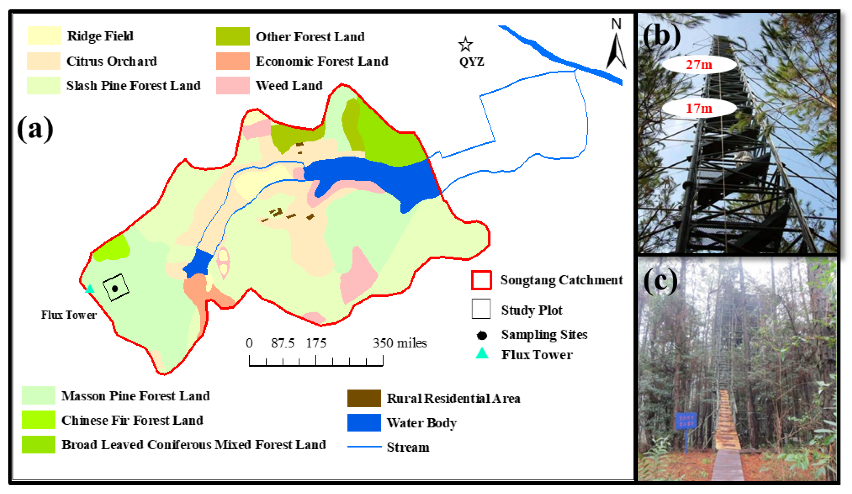
The study plot (100 × 100 m²) is located at the top of a hill within the Songtang catchment of QYZ (Figure 1a), where soil depth is less than 100 cm and the average groundwater level is about 3.43 m. The soil at the site is red earth weathered from sandstone, sandy conglomerate, mudstone, and alluvium. Soil bulk density is about 1.57 g cm⁻³, and sand, silt, and clay contents are 17, 68, and 15%, respectively [27]. The subtropical forest plantation at the site was planted in 1985, and the dominant tree species were Masson pine (Pinus massoniana L.), slash pine (Pinus elliottii E.), and Chinese fir (Cunninghamia lanceolata L.) [28]. According to a survey conducted in the study plot in 2011, canopy height was 14.4 m and the proportion of living numbers for P. massoniana (Pinus massoniana L.), P. elliottii (Pinus elliottii E.), C. lanceolata (Cunninghamia lanceolata L.), and other broadleaf trees were 50.0, 30.4, 7.5, and 12.1%, respectively. The growing season lasts from March to October.

2.2. In-Situ Measurements of Isotope Ratios in Water Vapor and Evapotranspiration

The in-situ system for measuring the δ¹⁸O and δ²H of atmospheric water vapor and their flux ratios consisted of a water vapor isotope analyzer (WVIA, Model DLT-100; Los Gatos Research Inc., San Jose, CA, USA) based on the isotope ratio infrared spectroscopy (IRIS) technique, an online calibration system, and an ambient air sampling system [8,29]. A water vapor isotope standard source (WVISS; Los Gatos Research Inc., San Jose, CA, USA) was used for the online calibration system, connecting the WVIA via a three-way solenoid valve. Five calibration gas streams (S1, S2, S3, S4, S5) with the same isotopic ratios and five mixing ratios were generated by a liquid vaporization module that instantaneously vaporized the standard water of a specific volume. The isotopic composition of the standard water was measured on a liquid water isotope analyzer (LWIA, Model DLT-100; Los Gatos Research Inc., San Jose, CA, USA). The switching sequence was calibration gas (S1, S2, S3, S4, S5), ambient air, calibration gas (S1, S2, S3, S4, S5), ambient air, with 5 min spent on each calibration gas and with 180 min spent on ambient air. The switch of the valve was controlled by an electric signal from WVIA.

The ambient air sampling system consisted of another three-way solenoid valve, a bypass pump, a sampling pump, and two buffer bottles. The δ¹⁸O_v profiles were measured at 17 m and 27 m above the canopy (Figure 1b). The switch between the two intakes for the measurement of the ambient air sample, with 2 min spent on each intake, was controlled by an electric signal from the WVIA. All of the sampling Teflon tubes were heated by a heating cable (Self-Regulating Heating Cable/Low Temperature, OMEGA Engineering Inc., Norwalk, CT, USA) and wrapped with heat-insulating materials to minimize the possibility of fractionation within the delivery tubes [30]. Flow rates of the bypass pump and sampling pump were 2.0 and 0.45 L min⁻¹ standard temperature and pressure (STP), respectively. Raw data were recorded at 1 Hz.

Two of the five calibration gases were selected to span the ambient water vapor concentration for calibrating ambient measurements. More details concerning the calibration procedure and the quality control of data are available in the literature [31,32]. Data after calibration were averaged in this study to hourly. The 1 h precision was ~0.2 ‰ for δ¹⁸O and ~0.4 ‰ for δ²H obtained by Allan variance analysis, which was given as one standard deviation of the difference between the measured isotope ratio and the value modeled according to the Rayleigh distillation equation with hourly averaging. The molar flux isotope ratio (R_ET) of evapotranspiration was determined by the flux-gradient technique using measurements at the two sampling heights above the canopy [31,33]. Here, R_ET was calculated on an hourly basis as:

$$R_{ET}=R_d\frac{x_{s,2}^{16}-x_{s,1}^{16}{x}_{a,2}^{18}-x_{a,1}^{18}}{x_{s,2}^{18}-x_{s,1}^{18}{x}_{a,2}^{16}-x_{a,1}^{16}}$$

(1)

where R_d is the molar ratio of the calibration water; x is the hourly mean mixing ratio of water isotopologues; superscripts 16 and 18 denote the ¹⁶O and ¹⁸O molecules in water, respectively; s,1 and s,2 indicate span calibration vapor streams of 1 (lower concentration) and 2 (higher concentration); and subscripts a,1 and a,2 represent ambient air sampled at height 27 m and 17 m. The molar ratio R_ET was converted to the standard δ (in ‰) in reference to the Vienna Standard Mean Ocean Water (VSMOW) as:

$${\delta }_{sample}(\raisebox{1ex}{$0$}\!\left/ \!\raisebox{-1ex}{$00$}\right.)=\left(\raisebox{1ex}{$R_{sample}$}\!\left/ \!\raisebox{-1ex}{$R_{VSMOW}$}\right.-1\right)\times 1000$$

(2)

where δ_sample is the δ¹⁸O and δ²H of ET; R_sample is the ratio of ¹⁸O/¹⁶O or ²H/¹H in ET; and R_VSMOW is the ratio of ¹⁸O/¹⁶O (0.0020052) or ²H/¹H (0.00015576) in VSMOW.

An above-canopy flux system for ecosystem evapotranspiration and CO₂ flux measurements was mounted on a tower at 39.6 m in the QYZ station (http://qya.cern.ac.cn, accessed on 18 May 2022). The flux system consisted of an open-path CO₂/H₂O analyzer (LI-7500, Licor Inc., Lincoln, NE, USA) and a three-dimensional sonic anemometer (CSAT3, Campbell Scientific Inc., Logan, UT, USA). Flux variables were sampled at 10 Hz using a CR5000 datalogger (Model CR5000, Campbell Scientific Inc., Logan, UT, USA), and 30 min mean fluxes were calculated [34]. Air temperature and relative humidity sensors (HMP45C, Campbell Scientific Inc., Logan, UT, USA) and wind speed sensors (A100R, Vector GB Ltd., Birmingham, UK) were installed at 1.6 m (ground layer), 15.6 m (canopy), and 23.6 m (above canopy). Net radiation was measured with Model CNR-1 (Kipp & Zonen Inc., Delft, The Netherlands) at 41.6 m. Air temperature, relative humidity, wind speed, and net radiation raw data were sampled at 10 Hz and the 30 min mean fluxes were calculated and stored on a CR5000 data logger (Campbell Scientific Inc., Logan, UT, USA) [35].

Soil volumetric water contents (SWC) were continuously measured at 5, 20, and 50 cm depths using three TDR probes (CS615-L, Campbell Scientific Inc., Logan, UT, USA) at a single location in the sampling plot to reflect the soil water condition of the soil sampling site. Soil temperatures were continuously measured at 5, 20, and 50 cm depths using three thermocouple temperature sensors (105T, Campbell Scientific Inc., Logan, UT, USA). Soil heat flux sensors (HFP01, Hukseflux, Delft, The Netherlands) were installed at 3 and 5 cm depths. Soil data were collected every 30 min with a CR10X data logger (Campbell Scientific Inc., Logan, UT, USA).

2.3. Measurement of Isotopic Compositions of Ecosystem Water Pools

Samples of xylem, leaf, and soil were taken starting at 02:00 18 October to 09:00 20 October 2011 at 3 or 4-h intervals for δ¹⁸O and δ²H isotopic analyses. There was no rain during the sampling period. For sampling xylem and leaf to represent the entire canopy, the three dominant tree species including C. lanceolata, P. massoniana, and P. elliottii in the study plot were selected based on plot survey data. Xylem was sampled from the south side of one mature tree per species [24]. These sampling trees were randomly selected around a bamboo tower (~12 m height, Figure 1c), which was used to facilitate the sampling of tree twigs. For each sample, phloem tissue was removed to avoid contamination by isotopically-enriched water [36]. Leaf samples were obtained from the same branch that was used for collecting the xylem samples. These samples were immediately cut into small segments, placed in vials, and sealed with parafilm. Soil samples at 0–5, 15–20, and 40–45 cm depths were collected with a hollow-stem auger (0.04 m in diameter and 0.25 m in length) and three replicate soil samples at each depth range were randomly taken in the sampling plot [37]. All samples were stored in a refrigerator at −15 °C to −20 °C until water extraction. Simultaneously, leaf temperature, specific leaf area, and leaf thickness of the three species were measured.

In total, 54 xylem, 54 leaf, and 162 soil samples were collected during the study period (Table S1). One week after sampling, water in xylem, leaf, and soil samples was extracted with a cryogenic vacuum distillation system, with heating at >90 °C and an extraction time of 0.5–1.5 h, depending on the water content of samples [38]. The extraction efficiency of water from the samples was >98.0% in this study. Xylem, leaf, and soil water was filtered through a 0.45 μm mixed cellulose membrane (Jiuding Gaoke Co. Ltd., Beijing, China), and 2 mL of water samples were used for the analysis of δ¹⁸O and δ²H. δ¹⁸O and δ²H were analyzed using LWIA. The number of injections into IRIS were 6 and the results of the last 3 injections were used for analysis. The results were normalized to VSMOW and expressed in the standard δ based on Equation (2). Using Equation (2), δ_sample is the δ¹⁸O and δ²H of the water sample and R_sample is the ratio of ¹⁸O/¹⁶O or ²H/¹H in the water sample. Commercial reference materials LGR3E, LGR5E, and LGR4 (Los Gatos Research Inc., San Jose, CA, USA) were used for quality control of IRIS. The measurement precision of the liquid water isotope analyzer was 0.1‰ for δ¹⁸O and 0.3‰ for δ²H [35].

2.4. Model and Statistical Methods

2.4.1. Simulation Models of Leaf Water, Transpiration, and Evaporation δ¹⁸O

To investigate the effects of δ¹⁸O_T on δ¹⁸O variability in atmospheric water vapor, we first considered leaf water ¹⁸O enrichment. The Craig–Gordon model [39] was first proposed for calculating the isotopic composition of evaporation water vapor from a liquid water surface as:

$${\delta }_E=\frac{{\delta }_L/{\alpha }_{eq}-h{\delta }_v-{\epsilon }_{eq}-(1-h){\epsilon }_k}{(1-h)+(1-h){\epsilon }_k/1000}$$

(3)

where subscripts E, L, and v represent the evaporating water vapor, liquid water body, and atmospheric water vapor, respectively; α_eq is the temperature-dependent equilibrium fractionation factor from liquid to vapor, and ε_eq = (1 − 1/α_eq) × 1000; h is the relative humidity of the ambient air referenced to the water surface temperature; ε_k is the kinetic fractionation factor.

The existing research reported that this model can be used to predict the leaf water enrichment [3,17,19]. Assuming that transpiration is in an isotopic steady-state (SS), namely δ¹⁸O_T is equal to xylem water δ¹⁸O (δ¹⁸O_x), and leaf water is isotopically well mixed, namely δ¹⁸O of bulk leaf water (δ_L,b) was equal to that at the evaporating site in the leaf (δ_L,e), and the Craig–Gordon model (CG, [39]) was developed as follows:

$${\delta }_{L,e}^s\approx {\delta }_{L,b}^s\approx {\delta }_x+{\epsilon }_{eq}+{\epsilon }_k+h({\delta }_v-{\epsilon }_k-{\delta }_x)$$

(4)

where superscript s denotes the steady state prediction; subscript x represents xylem water; δ_v is δ¹⁸O of atmospheric water vapor over the canopy (δ¹⁸O_v at 17 m); α_eq is the temperature-dependent equilibrium fractionation factor from liquid to vapor calculated with canopy temperature, and ε_eq = (1 − 1/α_eq) × 1000; h is the relative humidity normalized to canopy temperature; ε_k is the kinetic fractionation factor given by:

$${\epsilon }_k=\frac{(1/(D_i/D)-1)r_c+(1/(D_i/D{)}^{2/3}-1)r_b}{r_a+r_b+r_c}$$

(5)

where r_a, r_b, and r_c are aerodynamic, boundary layer, and canopy resistance, respectively. The term D_i/D is the ratio between the molecular diffusion coefficients of the heavy and light isotopes in air. The commonly accepted value of D_i/D(¹⁸O) is 0.9723 provided by Merlivat [40] and Farquhar et al. [41] with 21 °C and 760 Hg mm, and, thus, 1/(D_i/D) − 1 = 28‰ and 1/(D_i/D)^2/3 − 1 = 19‰. No fractionation occurs during turbulent diffusion in the atmospheric surface layer [42]. Above all, δ_L,b simulated by the CG model depended on δ¹⁸O_x, δ_v, h, ε_eq, and ε_k. The CG model has been used to simulate the diurnal variability of δ_L,b, and it was found that the CG model underestimated δ_L,b when there was less transpiration at night because SS was not fulfilled, namely δ¹⁸O_T was not equal to δ¹⁸O_x [13,17,19].

Numerous modeling and experimental studies have shown that the steady-state occurs only during a short period (hourly) near midday or in shorter canopies [9,10,17,19,43]. Therefore, the Dongmann model (DG, [17]) expresses the isotopic enrichment of leaf water considering non-steady-state effects and retained the assumption that δ_L,b was equal to δ_L,e as:

$${\delta }_{L,e}\approx {\delta }_{L,b}={\delta }_{L,b}^s+({\delta }_{L,b}^0-{\delta }_{L,b}^s)e^{-t/\tau }$$

(6)

$$\tau =\frac{W{\alpha }_k{\alpha }_{eq}}{g{w}_i}$$

(7)

where δ⁰_L,b is δ_L,b at time zero; W is the leaf water content (mol m⁻² leaf) and obtained by leaf samples; α_k is the fractionation factor of diffusion (α_k = 1 + ε_k/1000); g is the leaf stomatal conductance (mol m⁻² s⁻¹); and w_i is the saturated water vapor at the temperature of the water at evaporation sites (mol mol⁻¹).

Leaf-scale measurements have shown that leaf water is not isotopically well mixed, and its δ¹⁸O is highest at evaporation sites in the leaf and lowest near the xylem [44,45]. The progressive enrichment from the xylem to the evaporation site maintains an isotopic gradient that drives the diffusion of H₂¹⁸O molecules in the opposite direction of mass water flow in the leaf, a phenomenon termed the Péclet effect [46]. The Farquhar–Cernusak model (FC, [19]), which takes the Péclet effect into account, is expressed as:

$${\delta }_{L,b}={\delta }_{L,b}^s-\frac{{\alpha }_k{\alpha }_{eq}}{g{w}_i}\times \frac{1-e^{-P}}{P}\times \frac{d(W\left({\delta }_{L,b}-{\delta }_x\right))}{dt}$$

(8)

$${\delta }_{L,e}={\delta }_{L,e}^s-\frac{{\alpha }_k{\alpha }_{eq}}{g{w}_i}\times \frac{d(W\times \frac{1-e^{-P}}{P}\times \left({\delta }_{L,e}-{\delta }_x\right))}{dt}$$

(9)

$$P=TL/CD$$

(10)

where P is the Péclet number; T is the transpiration rate (mol m⁻² s⁻¹), obtained by the Shuttleworth–Wallace model; L is an effective path length for water movement through the mesophyll (m); and L have been difficult to determine directly, and, generally, been fitted using the observed and the predicted δ¹⁸O_L,b. The existing values of L for different species have been reported as 2.3 × 10⁻¹²–150 mm, and the optimized value of L was 100 mm for the three species and canopy levels in this study. C is the molar concentration of water (5.55 × 10⁴ mol m⁻³); and D is the temperature-dependent diffusivity of the heavy isotopologue in water (m² s⁻¹) [47]. Thus, P depends on T, L, and canopy temperature. When the limit of P→0 with T→0 mol m⁻² s⁻¹ or L→0 mm, Equations (8) and (9) reduce to δ_L,e = δ_L,b, or the well-mixed condition.

Under the steady-state assumption, δ¹⁸O_T is equal to xylem water δ¹⁸O (δ¹⁸O_x). In non-steady-state conditions, δ¹⁸O_T can deviate from δ¹⁸O_x and δ¹⁸O_T can be calculated with the CG model (Equation (3)). When simulating δ¹⁸O_T with Equation (3), δ_E means δ¹⁸O_T, and δ_L means δ_L,e. δ_L,e can be predicted by DG and FC models. The values of other parameters were the same as above. In this study, we also used the model of Hu et al. [8] for estimating δ¹⁸O_T, which was developed using the mass conservation principle at the ecosystem level as:

$${\delta }^{18}{O}_T=\frac{[{\delta }_x(T+\Delta W)-\Delta ({\delta }_{L,b}W)]}{T}$$

(11)

In this study, we linearly interpolated measured δ¹⁸O_L,b, δ¹⁸O_x, and W to 1 h resolution, assuming that they remained constant over a 1-h period. δ¹⁸O_L,b, δ¹⁸O_L,e, and δ¹⁸O_T of three species including C. lanceolata, P. massoniana, and P. elliottii were calculated. In addition, δ¹⁸O_L,b, δ¹⁸O_L,e, and δ¹⁸O_x of canopy levels were also estimated using the leaf or stem biomass–weight average method in this study, respectively. The proportion of leaf biomass per species was 33.8, 58.1, and 8.1%, and the proportion of stem biomass was 52.6, 43.8, and 3.6% for P. massoniana, P. elliottii, and C. lanceolata, respectively.

The evaporation δ¹⁸O (δ¹⁸O_E) was also estimated based on the CG model with Equation (3). When simulating δ¹⁸O_E by Equation (3), δ_E means δ¹⁸O_E, and δ_L means δ_s, which represents the isotopic composition of liquid water at the evaporating front, approximated here by the isotopic composition of soil water at the 0–5 cm depth. α_eq is the temperature-dependent equilibrium fractionation factor from liquid to vapor calculated with soil temperature at 5 cm depth; h is the relative humidity normalized to soil temperature at 5 cm depth; and ε_K is the kinetic fractionation factor calculated by Equation (5). When calculating the ε_K by Equation (5), r_c means soil resistance (r_s). r_a, r_b, r_c, and r_s were calculated using data acquired from the tower system measurements according to the methods of Lee et al. [42] and Xiao et al. [48]. In this study, we linearly interpolated measured δ¹⁸O_s to 1 h resolution, assuming that they remained constant over a 1-h period.

2.4.2. Calculations of Transpiration, Evaporation, and Evapotranspiration Isoforcing

To quantify the impact of transpiration (δ¹⁸O_T), evaporation (δ¹⁸O_E), and evapotranspiration δ¹⁸O (δ¹⁸O_ET) on δ¹⁸O_v, transpiration (I_T), evaporation (I_E), and evapotranspiration (I_ET) isoforcing, also called isoflux, was defined as the product of transpiration (T), evaporation (E), and evapotranspiration (ET) flux, and the deviation of their isotopic ratios from that of atmospheric water vapor, given by [10]:

$$I_T=T({\delta }^{18}{O}_T-{\delta }^{18}{O}_v)$$

(12)

$$I_E=E({\delta }^{18}{O}_E-{\delta }^{18}{O}_v)$$

(13)

$$I_{ET}=ET({\delta }^{18}{O}_{ET}-{\delta }^{18}{O}_v)$$

(14)

ET was measured by the above-canopy flux system mounted on the flux tower at 39.6 m (Details in Section 2.2). ET was partitioned as T and E by using the Shuttleworth–Wallace model (Details in Section 2.4.3).

2.4.3. The Shuttleworth–Wallace Model: Estimates of Transpiration and Evaporation

The Shuttleworth–Wallace (S–W) model is a variation of the Penman–Monteith model constrained by energy conservation, simulating soil evaporation and canopy transpiration at hourly time resolution [12]. The model takes into consideration the different resistances encountered by soil evaporation and canopy transpiration. In this study, the S–W model was coupled with a photosynthesis–stomatal (g_s–A_c) conductance sub-model developed by Ronda et al. [49] to calculate canopy transpiration. Mathematical details of the S–W model and the photosynthesis–stomatal conductance sub-model can be found in Wei et al. [12]. The input data of the S–W model included air temperature, relative humidity, net radiation, wind speed, atmospheric CO₂ concentration, air pressure, soil temperature and moisture, leaf area index (LAI), and canopy height. These input data except LAI were obtained by in-situ measurement (Details in Section 2.2). The MODIS LAI product (MCD15A3H), which has a spatial resolution of 250 m and a time resolution of 8 days, was downloaded from the National Aeronautics and Space Administration (NASA) website (https://modis.gsfc.nasa.gov/data/) (accessed on 18 May 2022). Validation was performed against the eddy covariance ET measurements and the slope and coefficient of variation (R²) of the regression line between observed and simulated ET were 0.90 and 0.86, respectively.

2.4.4. Statistical Analyses

The slope and coefficient of variation of linear regression between observed and simulated values, and root mean square error (RMSE) were used for evaluation of the models’ performance. Linear regression was also used for analyzing correlations between δ¹⁸O_v and environmental factors. Linear regression was conducted with SPSS 22.0 software (International Business Machines Corporation, Armonk, New York, USA, 2013). p < 0.05 was considered statistically significant at a 95% confidence interval. Pearson correlation coefficients were calculated using R studio 3.5.0 (RStudio Inc., Boston, MA, USA, 2009).

3. Results

3.1. Observed and Modeling Results of Leaf Water δ¹⁸O

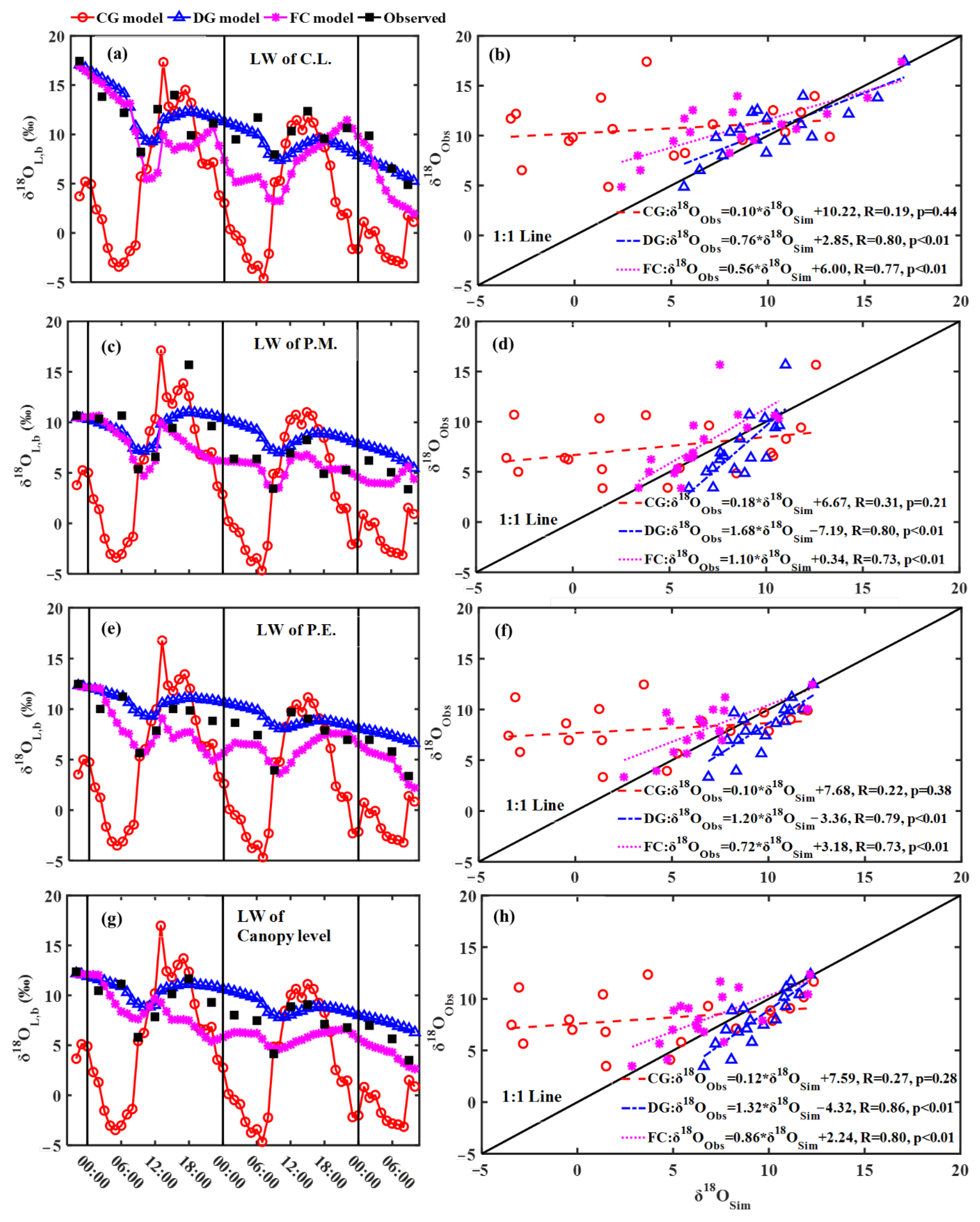
Observed δ¹⁸O of bulk leaf water (δ¹⁸O_L,b) gradually decreased in the morning, increased from 09:00 to 18:00, and then decreased at night (Figure 2 and Figure S1). These observed diurnal variations were reproduced reasonably by the three models. However, δ¹⁸O_L,b of C. lanceolata (Figure 2a,b), P. massoniana (Figure 2c,d), P. elliottii (Figure 2e,f), and canopy level (Figure 2g,h) simulated with the CG model with the steady-state assumption underestimated the observed δ¹⁸O_L,b for the morning and night. Between 09:00 and 18:00, values were similar between the CG-model simulated δ¹⁸O_L,b of C. lanceolata, P. elliottii, and canopy level and observed δ¹⁸O_L,b, but δ¹⁸O_L,b of P. massoniana simulated with the CG model still underestimated observed δ¹⁸O_L,b. The discrepancy between observed and simulated δ¹⁸O_L,b was greatly reduced by using the DG model with the non-steady-state assumption (R = 0.79–0.86; RMSE = 1.86–2.42). However, δ¹⁸O_L,b of P. massoniana simulated with the DG model overestimated observed δ¹⁸O_L,b (Figure 2c,d).

The FC model with the non-steady-state and the Péclet effect did not improve on the discrepancy between observed and simulated δ¹⁸O_L,b of C. lanceolata (RMSE_FC = 3.41‰ and RMSE_DG = 1.86‰) and P. elliottii (RMSE_FC = 2.16‰ and RMSE_DG = 2.06‰). The simulation performance of δ¹⁸O_L,b of P. massoniana was improved (RMSE_FC = 2.31‰ and RMSE_DG = 2.42‰), and the slope of the regression line between observed and simulated δ¹⁸O_L,b was changed from 1.68 with the DG model to 1.10 with the FC model. For canopy level, the simulation performance of δ¹⁸O_L,b with the FC model was similar to that obtained with the DG model (RMSE_FC = 1.97‰, and RMSE_DG = 1.86‰).

In general, predicted leaf water δ¹⁸O provides a basis for estimating δ¹⁸O_T (Equation (10)). Therefore, simulation of δ¹⁸O_T for the three species benefits from using δ¹⁸O_L,e simulated by the non-steady-state model, and δ¹⁸O_L,e simulated by considering the Péclet effect should be used for P. massoniana.

3.2. Modeling Results of Transpiration δ¹⁸O

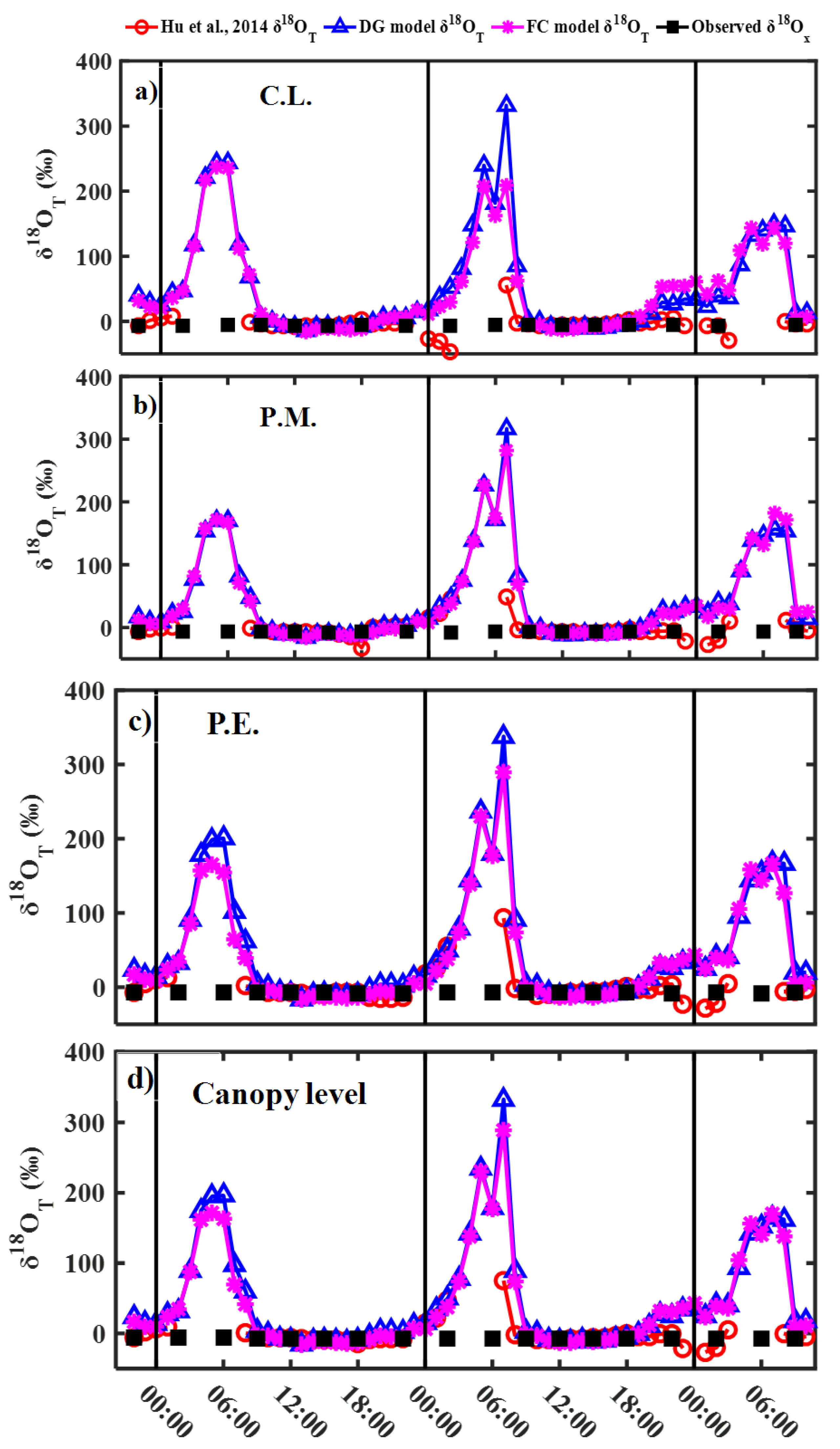
For comparing the effects of steady and non-steady-state assumption, and the Péclet effect on estimating δ¹⁸O_T, δ¹⁸O_T was calculated by the steady-state assumption (xylem water δ¹⁸O, δ¹⁸O_x), the Equation (10) with δ¹⁸O_L,e simulated by the DG and FC model, and the method of Hu et al. (2014). Before 12:00, δ¹⁸O_T obtained by simulated δ¹⁸O_L,e with the DG model (δ¹⁸O_TDG) and δ¹⁸O_T obtained by simulated δ¹⁸O_L,e with the FC model (δ¹⁸O_TFC) first increased, then decreased, and were significantly more than δ¹⁸O_T based on the steady-state assumption (δ¹⁸O_SS) (Figure 3). δ¹⁸O_TDG, δ¹⁸O_TFC, and δ¹⁸O_T simulated with the method of Hu et al. (2014) approached the steady-state value between 12:00 and 15:00 and was similar to δ¹⁸O_SS (Figure 3). After 18:00, δ¹⁸O_TDG, and δ¹⁸O_TFC gradually increased and its difference with δ¹⁸O_SS increased (Figure 3). However, the method of Hu et al. (2014) was not suitable for simulating δ¹⁸O_T at night with low transpiration rates. Diurnal variation pattern of δ¹⁸O_TDG was similar to that of δ¹⁸O_TFC for the three species and canopy level (Figure 3). However, the difference between δ¹⁸O_TDG and δ¹⁸O_TFC of C. lanceolata, P. elliottii, and the canopy level was larger than that of P. massoniana.

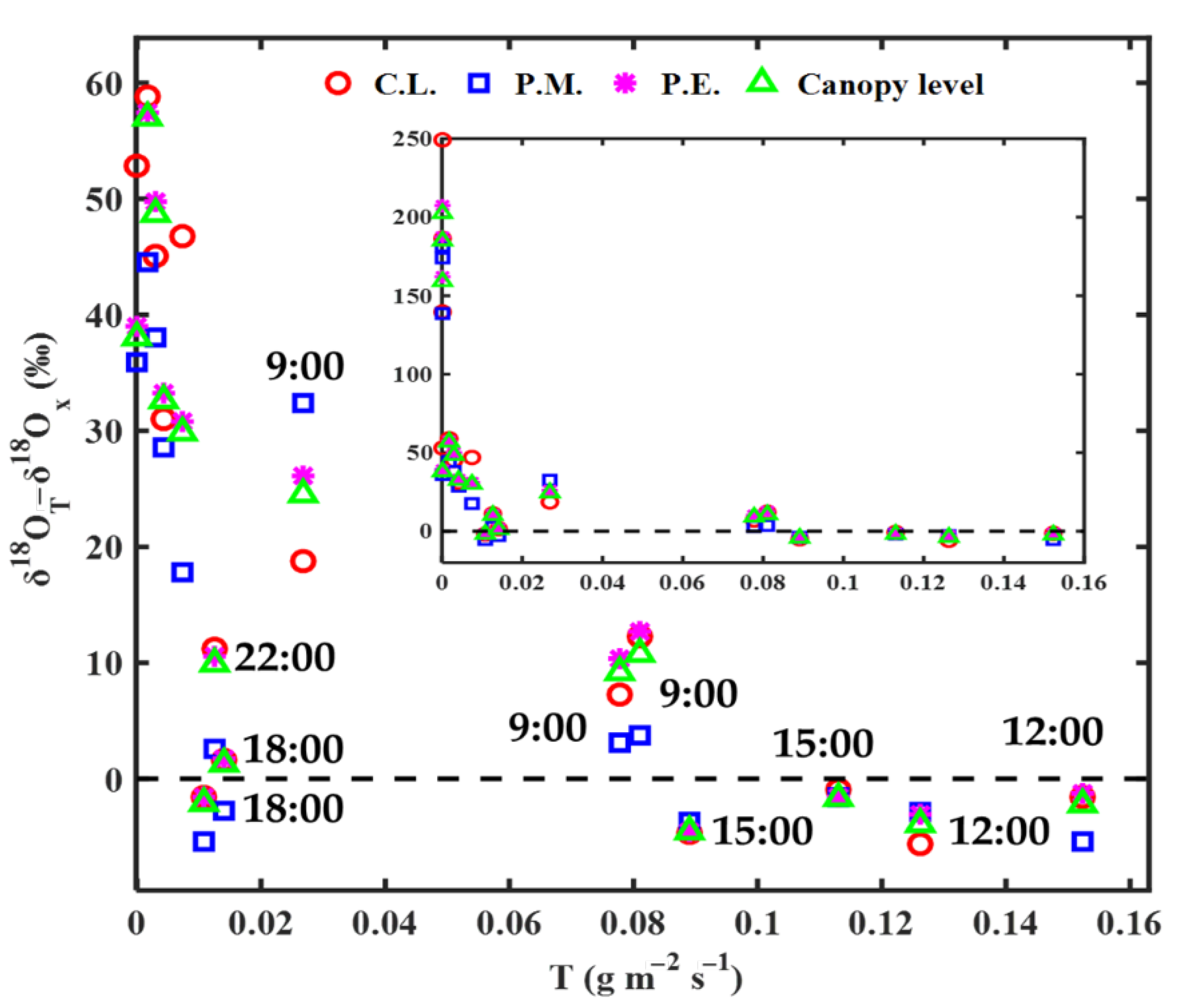
Based on Figure 4, the difference between δ¹⁸O_T based on non-steady-state assumption (δ¹⁸O_TNSS) and observed δ¹⁸O_x (δ¹⁸O_T−δ¹⁸O_x) decreased with an increase of transpiration rate. δ¹⁸O_T−δ¹⁸O_x was >7‰ for all species before 12:00, except δ¹⁸O_T−δ¹⁸O_x of P. elliottii at 09:00 (Figure 4). Between 12:00 and 15:00, δ¹⁸O_T−δ¹⁸O_x was <6‰. δ¹⁸O_T−δ¹⁸O_x after 18:00 was >9‰. In all, δ¹⁸O_T−δ¹⁸O_x was close to 0 with large transpiration rates, and, thus, the isotopic steady-state assumption was satisfied between 12:00 and 15:00. Except for 18:00, δ¹⁸O_T−δ¹⁸O_x was close to 0 with a low transpiration rate. This diurnal variability in the difference between δ¹⁸O_TNSS and observed δ¹⁸O_x were also shown in many existing pieces of research [3].

3.3. Diurnal Variability in Water Vapor δ¹⁸O and Its Controlling Factors

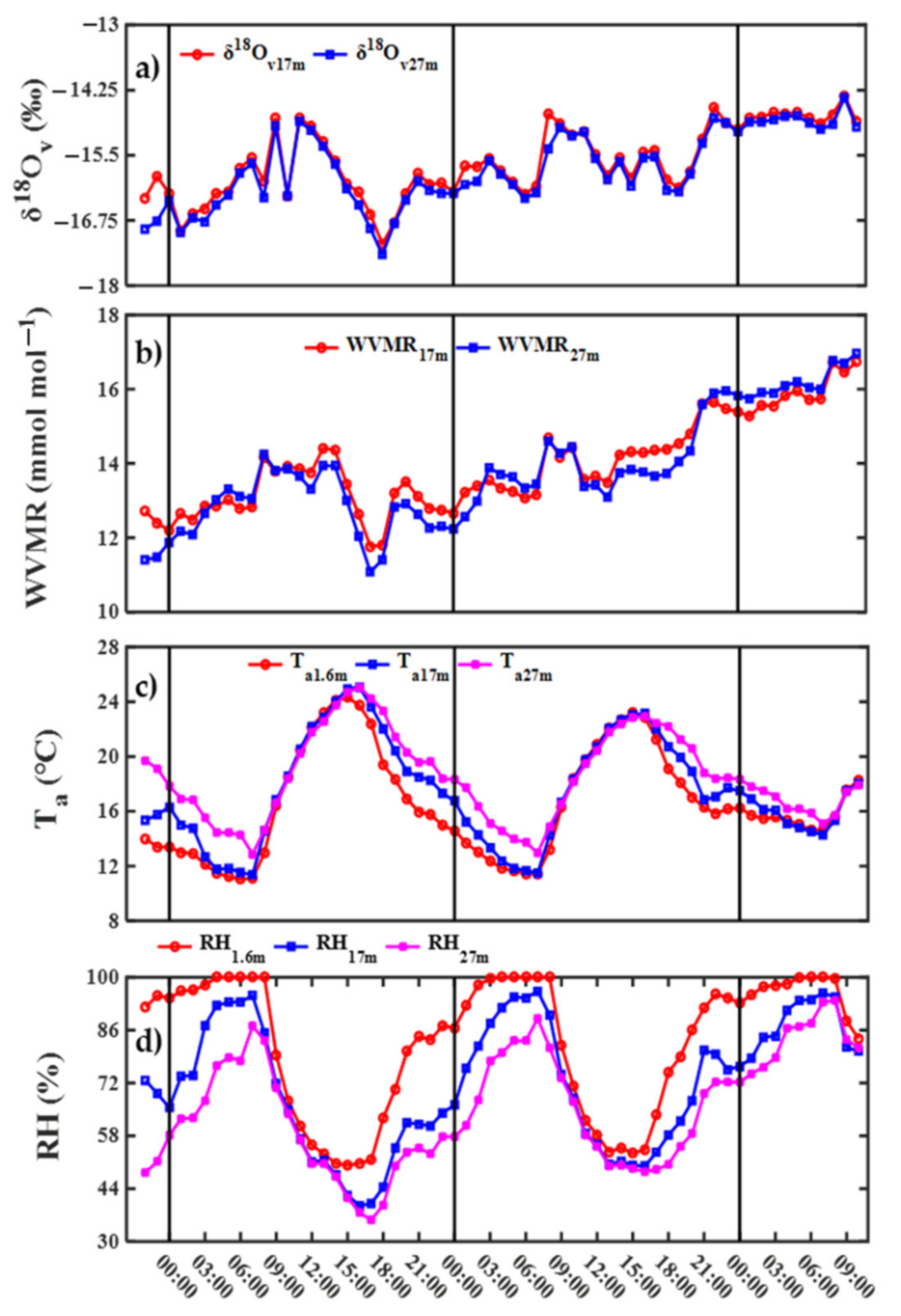
Diurnal variability of 2.4‰ in water vapor δ¹⁸O (δ¹⁸O_v) over the course of a day was consistently detected at 17 and 27 m on 18 October δ¹⁸O_v gradually increased before 09:00 and decreased at 10:00, first increased, and then decreased between 11:00 and 18:00, and then gradually increased after 18:00 (Figure 5a and Figure S1). Diurnal variability of 1.7‰ in δ¹⁸O_v over the course of a day on 19 October was lower than that on 18 October. The diurnal pattern before 08:00 on 19 October. was different from that on 18 October and δ¹⁸O_v first increased and then decreased. On 19 October, δ¹⁸O_v first increased then decreased between 08:00 and 18:00, and then gradually increased after 18:00.

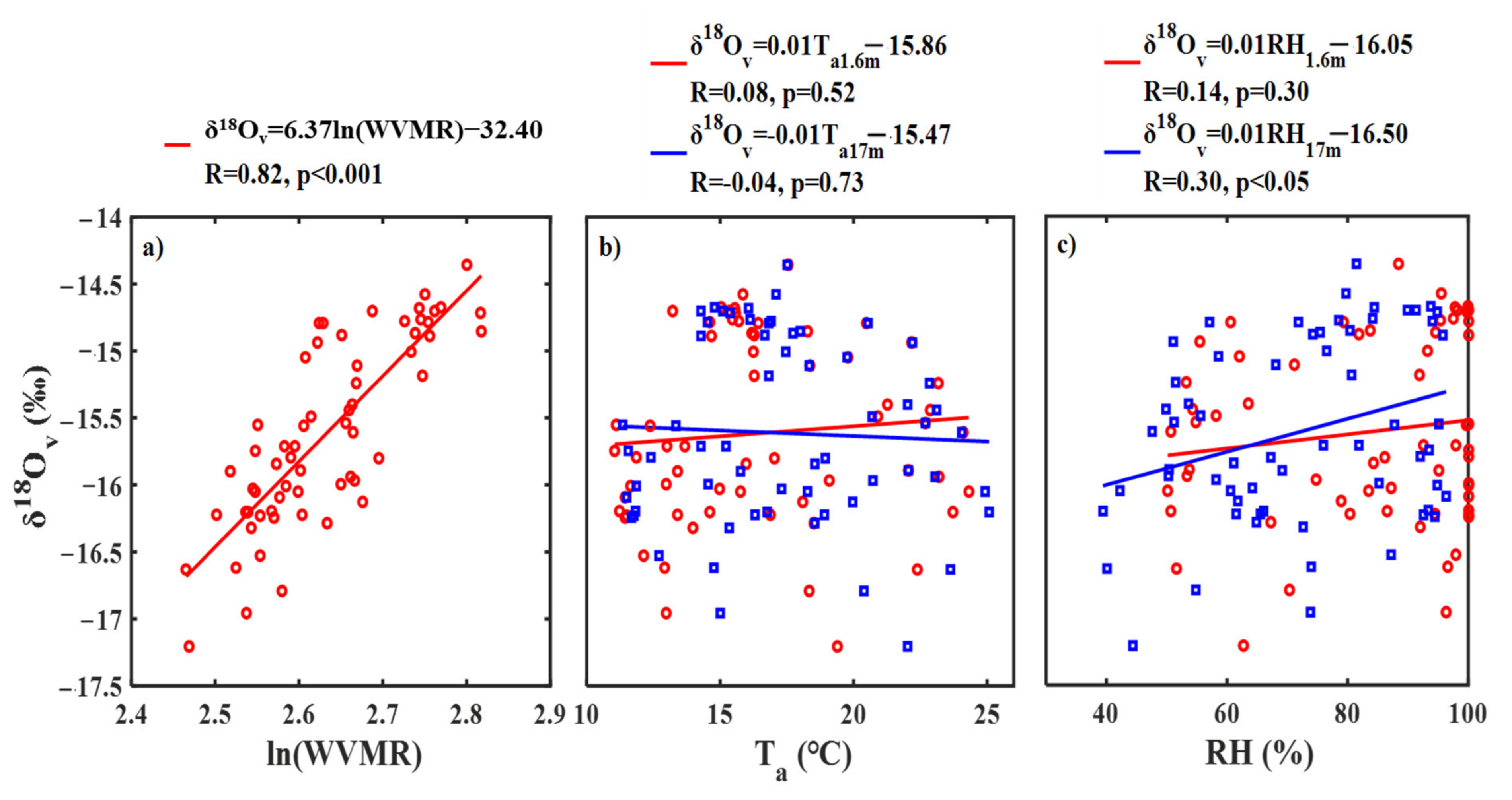
Water vapor mixing ratio (WVMR) at 17 and 27 m gradually increased before 09:00, approached a steady state between 09:00 and 14:00, gradually decreased between 14:00 and 18:00, and first increased and then decreased after 18:00 on 18 October (Figure 5b). On 19 October, WVMR first increased and then decreased, increased before 09:00, and approached a steady state between 09:00 and 11:00, first decreased and then approached a steady state between 12:00 and 15:00, and gradually increased after 15:00. There was a significant positive and log-linear relationship (δ¹⁸O_v = 6.37 ln(WVMR) − 32.40, R = 0.82) between δ¹⁸O_v and WVMR (Figure 6a). The log-linear relationship illustrated that Rayleigh processes provided an explanation for the observed diurnal pattern in δ¹⁸O_v at 17 m [9]. The Rayleigh processes may be attributed to the mixing with the atmosphere above the canopy (sourced from air advection) and atmospheric entrainment in no rain conditions.

Diurnal pattern in air temperature (T_a, Figure 5c) and relative humidity (RH, Figure 5d) at 1.6 m (ground layer), 17 m (canopy), and 27 m on 18 and 19 October was similar. T_a gradually decreased before 07:00, increased between 07:00 and 15:00, and decreased after 15:00. However, there was no significant correlation between T_a at the ground layer (related to equilibrium fractionation of soil evaporation) and canopy (related to equilibrium fractionation of transpiration) and δ¹⁸O_v (Figure 6b). Diurnal patterns in RH and T_a were opposite (Figure 5d). Although there were no significant correlations between RH at the ground layer (related to kinetic fractionation of soil evaporation) and δ¹⁸O_v, there was a significant correlation between RH at the canopy (related to kinetic fractionation of transpiration) and δ¹⁸O_v (Figure 6c). Therefore, besides Rayleigh processes, surface transpiration can also contribute to the observed diurnal pattern in δ¹⁸O_v, and the significant correlations between δ¹⁸O_v and leaf water δ¹⁸O can illustrate the contribution of transpiration to δ¹⁸O_v (Table S2).

3.4. Transpiration, Evaporation, and Evapotranspiration Isoforcing

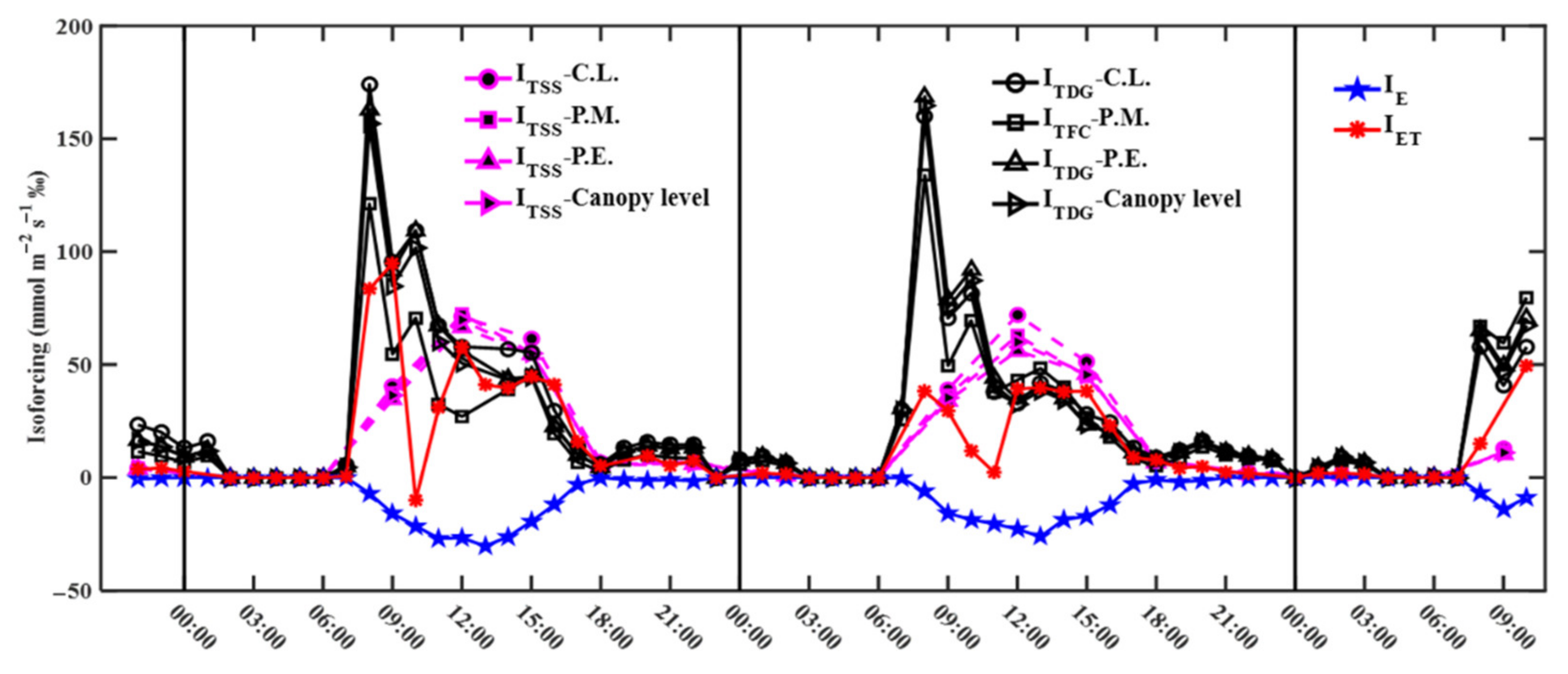
Transpiration (T) isoforcing via non-steady (I_TDG, calculated by δ¹⁸O_T which were obtained by using simulated δ¹⁸O_L,e with the DG model, and I_TFC, calculated by δ¹⁸O_T which were obtained by using simulated δ¹⁸O_L,e with the FC model) and steady-state (I_TSS) exerted positive isotope forcing on δ¹⁸O_v over the course of a day. The positive T isoforcing may be because the transpired water vapor becomes isotopically enriched when the isotopically-enriched soil water and leaf water are in the leaf mix (Figure S2) [50]. I_TDG and I_TFC were small before 06:00 (18 October) and 07:00 (19 October) and their average values were 2–4 (18 October) and 3–4 (19 October) mmol m⁻² s⁻¹ ‰ for three species and canopy level (Figure 7). I_TDG and I_TFC first increased and then decreased between 07:00 and 18:00 and reached maximum values of 121–174 (18 October) and 134–169 (19 October) mmol m⁻² s⁻¹ ‰ at 08:00, with average values of 38–61 (18 October) and 42–49 (19 October) mmol m⁻² s⁻¹ ‰ for three species and canopy level. I_TDG and I_TFC were also small after 18:00 with average values of 7–12 (18 October) and 10–12 (19 October) mmol m⁻² s⁻¹ ‰ for three species and canopy level. I_TSS before 06:00 and after 18:00 was also small and lower than I_TDG and I_TFC. Between 07:00 and 18:00, I_TSS also first increased and then decreased and reached maximum values of 66–72 (18 October) and 56–72 (19 October) mmol m⁻² s⁻¹ ‰ at 12:00, with average values of 40–45 (18 October) and 36–42 (19 October) mmol m⁻² s⁻¹ ‰ for three species and canopy level. In general, T isoforcing was similar via non-steady and steady-state between 12:00 and 18:00, while non-steady-state was higher than steady-state before 12:00 and after 18:00.

Soil evaporation (E) had the opposite effect and tended to decrease δ¹⁸O_v during the day (Figure 7). This may be because the evaporation of soil water releases isotopically depleted water vapor compared to δ¹⁸O_v (Figure S3) [50]. E isoforcing (I_E) was at about 0 mmol m⁻² s⁻¹ ‰ before 07:00 and after 18:00. I_E first increased and then decreased between 07:00 and 18:00 and reached maximum absolute values of 30 (18 October) and 26 (19 October) mmol m⁻² s⁻¹ ‰ at 13:00, with average absolute values of 19 (18 October) and 16 (19 October) mmol m⁻² s⁻¹ ‰. Evapotranspiration isoforcing (I_ET) before 07:00 and after 18:00 was small and similar to that of T and E (Figure 7). I_ET presented an M-shaped distribution between 07:00 and 18:00 and the two maxima were 95 mmol m⁻² s⁻¹ ‰ at 09:00 and 58 mmol m⁻² s⁻¹ ‰ at 12:00 on 18 October, and 38 mmol m⁻² s⁻¹ ‰ at 08:00 and 40 mmol m⁻² s⁻¹ ‰ at 13:00 on 19 October. Therefore, I_ET reflected the integrated results of T and E and the former was more important.

4. Discussion

4.1. Effects of Steady and Non-Steady-State Assumption, and the Péclet Effect on Estimating δ¹⁸O_T

Existing research has shown that the isotopic steady-state (SS) only occurs during a short period (hourly) near midday when the turnover time of leaf water is short [7,13]. Under the assumptions of thin leaves, quick leaf water turnover and uniformly distribute isotope, the water mass of transpiration is much higher than that of the leaf water, and, thus, the isotopic composition of water exiting the leaves is equal to that entering the leaves, namely δ¹⁸O_T = δ¹⁸O_x [3,51]. In this study, δ¹⁸O_TDG and δ¹⁸O_TFC were closer to δ¹⁸O_x at midday between 12:00 and 15:00 (Figure 3 and Figure 4) when the transpiration rate was high (Figure 4 and Figure S3) and the turnover time of leaf water was short (0.4–1.8 h). However, δ¹⁸O_TDG and δ¹⁸O_TFC were significantly higher than δ¹⁸O_x in the morning and at night when the transpiration rate was low, and the turnover times of leaf water were long (5.23–80.15 h) (Figure 3). This illustrated that SS was satisfied between 12:00 and 15:00 [10] and SS would underestimate δ¹⁸O_T in the morning and at night. Although the turnover time of leaf water was long (4.82–13.13 h) at 18:00, δ¹⁸O_T based on non-steady-state effects (NSS) was closer to δ¹⁸O_x. This may be due to uncertainties associated with estimating δ¹⁸O_T based on NSS [8].

Several publications have pointed out that NSS of δ¹⁸O_T in the mornings and at night would be more significant than those in the middle of the day due to low transpiration rates and long turnover times of leaf water [6,9]. When transpiration rate is low and leaf water concentrations are high, δ¹⁸O_T may be more enriched than δ¹⁸O_x due to the accumulation of isotopically-enriched leaf water [9,52]. In this study, there was evidence of NSS after 18:00 and before 12:00 (Figure 3). δ¹⁸O_TDG and δ¹⁸O_TFC were higher than δ¹⁸O_x during those periods and first increased and then decreased (Figure 3). Long turnover times of leaf water (5.23–80.15 h) may lead to enriched δ¹⁸O_L,b due to transpiration in the afternoon accumulating in the leaf water and increased δ¹⁸O_T between 18:00 and 06:00 [9,16]. After 06:00, absorption of depleted soil water by roots may lead to depletion of δ¹⁸O_L,b, and a decrease in δ¹⁸O_T because water uptake by roots was greater than water loss by transpiration [6,53].

Many experimental studies have confirmed the existence of the Péclet effect, namely leaf water is not thoroughly mixed and a gradual decrease of leaf water ¹⁸O occurs from the evaporation sites to leaf veins [13,18]. Due to the Péclet effect, simulated leaf water ¹⁸O with the assumptions of uniformly distributed isotope may always be higher than the observed values [3]. In this study, δ¹⁸O_L,b simulated with the DG model was higher than δ¹⁸O_L,b simulated with the FC model and, thus, δ¹⁸O_TDG also was higher than δ¹⁸O_TFC (Figure 2 and Figure 3). However, the FC model improved the simulation performance of δ¹⁸O_L,b of P. massoniana but not of δ¹⁸O_L,b of C. lanceolata or P. elliottii, compared with the DG model (Figure 2). There were two reasons for the discrepancy: (1) leaves of P. massoniana may have a stronger Péclet effect than those of C. lanceolata and P. elliottii; (2) the FC model is not suitable for simulating δ¹⁸O_L,b of C. lanceolata and P. elliottii.

On the one hand, the Péclet effect in the FC model was mainly affected by the effective path length for water movement through the mesophyll (L), transpiration rate, and canopy temperature [19]. Leaf temperatures of the three species were similar and the same as canopy temperature. Due to the similar stomatal conductance of the three species [54], the same transpiration rate was assumed. Therefore, this discrepancy may be mainly because the differences in leaf anatomy between species lead to the differences in the pathways of water movement within the leaf [7]. Specific leaf areas of C. lanceolata, P. massoniana, and P. elliottii were 10.53 m² kg⁻¹, 8.70 m² kg⁻¹, and 6.71 m² kg⁻¹, and their leaf thickness were 0.28 mm, 0.53 mm, and 0.77 mm, respectively. The existing research found that if multiple parallel pathways in the liquid phase obscure the Péclet effect at the bulk leaf level, then leaves with a high proportion of vapor phase transport and few parallel liquid pathways would have a stronger Péclet effect. The different leaf anatomy of P. massoniana may lead to a strong Péclet effect, compared to C. lanceolata and P. elliottii.

On the other hand, changes in L and the location of evaporating surfaces with the change in transpiration rate were not considered in the FC model. These assumptions may be not suitable for C. lanceolata and P. elliottii due to their leaf anatomy. However, the reason for the differences in the Péclet effect among the three species needs to be further studied. The Péclet effect was less important to leaf water ¹⁸O enrichment than the non-steady-state effect at the canopy level. It indicated that the implicit assumptions of the DG model—that the ¹⁸O content is well mixed in leaf water—are good approximations for canopy-level applications [13].

4.2. Effects of δ¹⁸O_T with Non-Steady-State Assumption on Atmospheric Water Vapor δ¹⁸O

Due to decreasing atmospheric vertical mixing and the appearance of an inversion layer, the most obvious local influence on δ¹⁸O_v was the positive T isoforcing in the morning and at night [10,22]. In this study, 1.43, 1.17, and 1.10‰ enrichment of δ¹⁸O_v was observed before 09:00 and after 18:00 on 18 October, and after 18:00 on 19 October, respectively (Figure 7). The enrichment of δ¹⁸O_v may be attributed to a significant amount of positive T isoforcing with 267 mmol m⁻² s⁻¹ ‰ (before 09:00 on 18 October), 56 mmol m⁻² s⁻¹ ‰ (after 18:00 on 18 October), and 64 mmol m⁻² s⁻¹ ‰ (after 18:00 on 19 October) mmol m⁻² s⁻¹ into the canopy. The decrease in atmospheric vertical mixing and the appearance of an inversion layer led to a greater contribution from positive T isoforcing and a lower contribution from the depleted atmosphere above the canopy [9,23]. The variability in air temperature and relative humidity with different observation heights indicated the appearance of an inversion layer (Figure 5). In addition, δ¹⁸O_v was first enriched by 0.64‰ and then depleted by 0.53‰ before 08:00 on 19 October. During this period, a decreasing difference between relative humidity at 1.6 and 27 m from 29% to 18% indicated that the inversion layer changed from strong to weak (Figure 5). Therefore, positive T isoforcing increased δ¹⁸O_v when the inversion layer was strong, while the depleted atmosphere above the canopy decreased δ¹⁸O_v when the inversion layer became weak.

The contribution from the positive T isoforcing first increased and then decreased during the daytime due to strong vertical mixing and a corresponding pattern in transpiration rate [9,22]. In this study, δ¹⁸O_v first increased and then decreased between 10:00 and 18:00 on 18 October (Figure 7). On the one hand, positive T isoforcing was higher than the negative E isoforcing and increased δ¹⁸O_v when the transpiration rate increased [9]. On the other hand, when vertical mixing was strong and transpiration rate decreased, the contribution from positive T isoforcing decreased and the contribution from the depleted atmosphere above the canopy increased, thus decreasing δ¹⁸O_v [22,23]. Similar results were also observed between 08:00 and 18:00 on 19 October. In addition, δ¹⁸O_v was depleted by 1.49‰ at 10:00 on 18 October and it may be due to the mixing of the depleted atmosphere above the canopy or negative ET isoforcing of −10 mmol m⁻² s⁻¹ (Figure 7).

In general, isotopic steady-state assumption underestimated the contribution from positive T isoforcing to δ¹⁸O_v in the morning and at night [9,10]. Namely, positive T isoforcing was underestimated with the assumption of isotopic steady state by 146 and 19 mmol m⁻² s⁻¹ on 18 October and by 172 and 38 mmol m⁻² s⁻¹ on 19 October before 09:00 and after 18:00, respectively (Figure 7). There were no significant differences in positive T isoforcing with the assumption of isotopic steady state and that with non-steady-state during 12:00 to 15:00. However, transpiration and evaporation fluxes and their isotope compositions have prominent seasonal variability in the subtropical regions, and, thus, diurnal patterns of T and E isoforcing during the different seasons may exist. The existing study found that the premonsoon season released a greater number of ¹⁸O into the atmosphere through the transpiration process, while during the monsoon season an increase in the ¹⁶O because of the incursion of the marine water vapor depleted in isotopic value of the atmosphere water vapor [53]. However, the change in diurnal patterns of transpiration and E isoforcing with the different seasons needs to be studied.

5. Conclusions

The results of this study indicate that the isotopic steady-state assumption was satisfied between 12:00 and 15:00 in this subtropical forest plantation. The non-steady-state effect was significant and δ¹⁸O_T was underestimated with the isotopic steady-state assumption before 12:00 and after 18:00 during the course of a whole day. The FC model improved the simulation performance of δ¹⁸O_L,b of P. massoniana, but not of δ¹⁸O_L,b of C. lanceolata or P. elliottii, compared with the DG model. At the canopy level, the Péclet effect was less important to leaf water ¹⁸O enrichment than the non-steady-state effect. The decreasing atmospheric vertical mixing and appearance of an inversion layer resulted in a greater contribution of positive T isoforcing to δ¹⁸O_v in the morning and at night. During the daytime, the contribution from positive T isoforcing first increased and then decreased due to strong vertical mixing and a similar pattern in transpiration rate. However, the isotopic steady-state assumption underestimated the contribution of positive T isoforcing to δ¹⁸O_v in the morning and at night. Our results highlight the importance of estimating δ¹⁸O_T via isotopic non-steady-state and the contribution of transpiration to atmospheric water vapor in the morning and at night.

References

- Brooks, J.R. Water, bound and mobile. Science 2015, 349, 138–139. [Google Scholar]
- Jasechko, S.; Sharp, Z.D.; Gibson, J.J.; Birks, S.J.; Yi, Y.; Fawcett, P.J. Terrestrial water fluxes dominated by transpiration. Nature 2013, 496, 347–350. [Google Scholar] [PubMed]
- Xiao, W.; Wei, Z.; Wen, X. Evapotranspiration partitioning at the ecosystem scale using the stable isotope method—A review. Agric. For. Meteorol. 2018, 263, 346–361. [Google Scholar]
- Gat, J.R. Oxygen and hydrogen isotopes in the hydrologic cycle. Annu. Rev. Earth Planet. Sci. 1996, 24, 225–262. [Google Scholar]
- Sprenger, M.; Leistert, H.; Gimbel, K.; Weiler, M. Illuminating hydrological processes at the soil-vegetation-atmosphere interface with water stable isotopes. Rev. Geophys. 2016, 54, 674–704. [Google Scholar]
- Cernusak, L.A.; Barbour, M.M.; Arndt, S.K.; Cheesman, A.W.; English, N.B.; Feild, T.S.; Helliker, B.R.; Holloway-Phillips, M.M.; Holtum, J.A.M.; Kahmen, A.; et al. Stable isotopes in leaf water of terrestrial plants. Plant Cell Environ. 2016, 39, 1087–1102. [Google Scholar]
- Barbour, M.M.; Farquhar, G.D.; Buckley, T.N. Leaf water stable isotopes and water transport outside the xylem. Plant Cell Environ. 2017, 40, 914–920. [Google Scholar]
- Hu, Z.M.; Wen, X.F.; Sun, X.M.; Li, L.H.; Yu, G.R.; Lee, X.H.; Li, S.G. Partitioning of evapotranspiration through oxygen isotopic measurements of water pools and fluxes in a temperate grassland. J. Geophys. Res.-Biogeo. 2014, 119, 358–371. [Google Scholar]
- Lai, C.T.; Ehleringer, J.R.; Bond, B.J.; Paw, U.K. Contributions of evaporation, isotopic non-steady state transpiration and atmospheric mixing on the δ18O of water vapour in Pacific Northwest coniferous forests. Plant Cell Environ. 2006, 29, 77–94. [Google Scholar]
- Welp, L.R.; Lee, X.; Kim, K.; Griffis, T.J.; Billmark, K.A.; Baker, J.M. δ18O of water vapour, evapotranspiration and the sites of leaf water evaporation in a soybean canopy. Plant Cell Environ. 2008, 31, 1214–1228. [Google Scholar]
- Simonin, K.A.; Link, P.; Rempe, D.; Miller, S.; Oshun, J.; Bode, C.; Dietrich, W.E.; Fung, I.; Dawson, T.E. Vegetation induced changes in the stable isotope composition of near surface humidity. Ecohydrology 2014, 7, 936–949. [Google Scholar]
- Wei, Z.W.; Lee, X.H.; Wen, X.F.; Xiao, W. Evapotranspiration partitioning for three agro-ecosystems with contrasting moisture conditions: A comparison of an isotope method and a two-source model calculation. Agric. For. Meteorol. 2018, 252, 296–310. [Google Scholar]
- Xiao, W.; Lee, X.H.; Wen, X.F.; Sun, X.M.; Zhang, S.C. Modeling biophysical controls on canopy foliage water 18O enrichment in wheat and corn. Glob. Change Biol. 2012, 18, 1769–1780. [Google Scholar]
- Flanagan, L.B.; Ehleringer, J.R. Effects of mild water stress and diurnal changes in temperature and humidity on the stable oxygen and hydrogen isotopic composition of leaf water in Cornus stolonifera L. Plant Physiol. 1991, 97, 298–305. [Google Scholar] [CrossRef]
- Yakir, D. Variations in the natural abundance of 18O and deuterium in plant carbohydrates. Plant Cell Environ. 1992, 15, 1005–1020. [Google Scholar]
- Cernusak, L.A.; Pate, J.S.; Farquhar, G.D. Diurnal variation in the stable isotope composition of water and dry matter in fruiting Lupinus angustifolius under field conditions. Plant Cell Environ. 2002, 25, 893–907. [Google Scholar]
- Dongmann, G.; Nurnberg, H.W.; Forstel, H.; Wagener, K. Enrichment of H218O in leaves of transpiring plants. Radiat. Environ. Biophys. 1974, 11, 41–52. [Google Scholar]
- Farquhar, G.D.; Gan, K.S. On the progressive enrichment of the oxygen isotopic composition of water along a leaf. Plant Cell Environ. 2003, 26, 801–819. [Google Scholar]
- Farquhar, G.D.; Cernusak, L.A. On the isotopic composition of leaf water in the non-steady state. Funct. Plant Biol. 2005, 32, 293–303. [Google Scholar]
- Welp, L.R.; Lee, X.; Griffis, T.J.; Wen, X.F.; Xiao, W.; Li, S.; Sun, X.; Hu, Z.; Val Martin, M.; Huang, J. A meta-analysis of water vapor deuterium-excess in the midlatitude atmospheric surface layer. Glob. Biogeochem. Cycles 2012, 26, GB3021. [Google Scholar]
- Schlesinger, W.H.; Jasechko, S. Transpiration in the global water cycle. Agric. For. Meteorol. 2014, 189, 115–117. [Google Scholar]
- Zhao, L.; Wang, L.; Liu, X.; Xiao, H.; Ruan, Y.; Zhou, M. The patterns and implications of diurnal variations in the d-excess of plant water, shallow soil water and air moisture. Hydrol. Earth Syst. Sci. 2014, 18, 4129–4151. [Google Scholar]
- Parkes, S.D.; McCabe, M.F.; Griffiths, A.D.; Wang, L.X.; Chambers, S.; Ershadi, A.; Williams, A.G.; Strauss, J.; Element, A. Response of water vapour D-excess to land-atmosphere interactions in a semi-arid environment. Hydrol. Earth Syst. Sci. 2017, 21, 533–548. [Google Scholar]
- Yang, B.; Wen, X.; Sun, X. Seasonal variations in depth of water uptake for a subtropical coniferous plantation subjected to drought in an East Asian monsoon region. Agric. For. Meteorol. 2015, 201, 218–228. [Google Scholar]
- Sun, X.; Wen, X.; Yu, G.; Liu, Y.; Liu, Q. Seasonal drought effects on carbon sequestration of a mid-subtropical planted forest of southeastern China. Sci. China Ser. D-Earth Sci. 2006, 49, 110–118. [Google Scholar]
- Yu, G.; Chen, Z.; Piao, S.; Peng, C.; Ciais, P.; Wang, Q.; Li, X.; Zhu, X. High carbon dioxide uptake by subtropical forest ecosystems in the East Asian monsoon region. Proc. Natl. Acad. Sci. USA 2014, 111, 4910–4915. [Google Scholar]
- Song, X.; Lyu, S.; Wen, X. Limitation of soil moisture on the response of transpiration to vapor pressure deficit in a subtropical coniferous plantation subjected to seasonal drought. J. Hydrol. 2020, 591, 125301. [Google Scholar]
- Song, X.W.; Lyu, S.D.; Sun, K.; Gao, Y.; Wen, X.F. Flux and source of dissolved inorganic carbon in a headwater stream in a subtropical plantation catchment. J. Hydrol. 2021, 600, 126511. [Google Scholar]
- Huang, L.; Wen, X. Temporal variations of atmospheric water vapor δD and δ18O above an arid artificial oasis cropland in the Heihe River Basin. J. Geophys. Res.-Atmos. 2014, 119, 11456–11476. [Google Scholar]
- Sturm, P.; Knohl, A. Water vapor δ2H and δ18O measurements using off-axis integrated cavity output spectroscopy. Atmos. Meas. Tech. 2010, 3, 67–77. [Google Scholar]
- Wen, X.F.; Lee, X.H.; Sun, X.M.; Wang, J.L.; Hu, Z.M.; Li, S.G.; Yu, G.R. Dew water isotopic ratios and their relationships to ecosystem water pools and fluxes in a cropland and a grassland in China. Oecologia 2012, 168, 549–561. [Google Scholar] [PubMed]
- Wen, X.F.; Sun, X.M.; Zhang, S.C.; Yu, G.R.; Sargent, S.D.; Lee, X.H. Continuous measurement of water vapor D/H and 18O/16O isotope ratios in the atmosphere. J. Hydrol. 2008, 349, 489–500. [Google Scholar]
- Lee, X.H.; Kim, K.; Smith, R. Temporal variations of the 18O/16O signal of the whole-canopy transpiration in a temperate forest. Glob. Biogeochem. Cycles 2007, 21, GB3013. [Google Scholar]
- Wen, X.F.; Yu, G.R.; Sun, X.M.; Li, Q.K.; Liu, Y.F.; Zhang, L.M.; Ren, C.Y.; Fu, Y.L.; Li, Z.Q. Soil moisture effect on the temperature dependence of ecosystem respiration in a subtropical Pinus plantation of southeastern China. Agric. For. Meteorol. 2006, 137, 166–175. [Google Scholar]
- Lyu, S.D.; Wang, J. Soil water stable isotopes reveal surface soil evaporation loss dynamics in a subtropical forest plantation. Forests 2021, 12, 1648. [Google Scholar]
- Querejeta, J.I.; Estrada-Medina, H.; Allen, M.F.; Jimenez-Osornio, J.J. Water source partitioning among trees growing on shallow karst soils in a seasonally dry tropical climate. Oecologia 2007, 152, 26–36. [Google Scholar]
- Lyu, S.D. Variability of δ2H and δ18O in soil water and its linkage to precipitation in an East Asian monsoon subtropical forest plantation. Water 2021, 13, 2930. [Google Scholar]
- Lyu, S.D.; Wang, J.; Song, X.W.; Wen, X.F. The relationship of δD and δ18O in surface soil water and its implications for soil evaporation along grass transects of Tibet, Loess, and Inner Mongolia Plateau. J. Hydrol. 2021, 600, 126533. [Google Scholar]
- Craig, H.; Gordon, L. Deuterium and oxygen-18 variations in the ocean and the marine atmosphere. In Stable Isotopes in Oceanographic Studies and Paleotemperatures; Tongiorgi, E., Ed.; Consiglio Nazionale delle Ricerche, Laboratorio di Geologia Nucleare: Spoleto, Italy, 1965. [Google Scholar]
- Merlivat, L. Molecular diffusivities of H216O, HD16O, and H218O in gases. J. Chem. Phys. 1978, 69, 2864–2871. [Google Scholar]
- Farquhar, G.D.; Ehleringer, J.R.; Hubick, K.T. Carbon isotope discrimination and photosynthesis. Annu. Rev. Plant Phys. 1989, 40, 503–537. [Google Scholar]
- Lee, X.H.; Griffis, T.J.; Baker, J.M.; Billmark, K.A.; Kim, K.; Welp, L.R. Canopy-scale kinetic fractionation of atmospheric carbon dioxide and water vapor isotopes. Glob. Biogeochem. Cycles 2009, 23, 15. [Google Scholar]
- Cernusak, L.A.; Farquhar, G.D.; Pate, J.S. Environmental and physiological controls over oxygen and carbon isotope composition of Tasmanian blue gum, Eucalyptus globulus. Tree Physiol. 2005, 25, 129–146. [Google Scholar] [PubMed]
- Helliker, B.R.; Ehleringer, J.R. Establishing a grassland signature in veins: 18O in the leaf water of C3 and C4 grasses. Proc. Natl. Acad. Sci. USA 2000, 97, 7894–7898. [Google Scholar] [PubMed]
- Yakir, D.; Sternberg, L.D.L. The use of stable isotopes to study ecosystem gas exchange. Oecologia 2000, 123, 297–311. [Google Scholar] [PubMed]
- Farquhar, G.D.; Lloyd, J. Carbon and oxygen isotope effects in the exchange of carbon dioxide between terrestrial plants and the atmosphere. In Book Carbon and Oxygen Isotope Effects in the Exchange of Carbon Dioxide between Terrestrial Plants and the Atmosphere; Academic Press: San Diego, CA, USA, 1993. [Google Scholar]
- Cuntz, M.; Ogée, J.; Farquhar, G.D.; Peylin, P.; Cernusak, L.A. Modelling advection and diffusion of water isotopologues in leaves. Plant Cell Environ. 2007, 30, 892–909. [Google Scholar]
- Xiao, W.; Lee, X.H.; Griffis, T.J.; Kim, K.; Welp, L.R.; Yu, Q. A modeling investigation of canopy-air oxygen isotopic exchange of water vapor and carbon dioxide in a soybean field. J. Geophys. Res.-Biogeo. 2010, 115, G01004. [Google Scholar]
- Ron da, R.J.; de Bruin, H.A.R.; Holtslag, A.A.M. Representation of the canopy conductance in modeling the surface energy budget for low vegetation. J. Appl. Meteorol. 2001, 40, 1431–1444. [Google Scholar]
- Chakraborty, S.; Burman, P.K.D.; Sarma, D.; Sinha, N.; Datye, A.; Metya, A.; Murkute, C.; Saha, S.K.; Sujith, K.; Gogoi, N.; et al. Linkage between precipitation isotopes and biosphere-atmosphere interaction observed in northeast India. npj Clim. Atmos. Sci. 2022, 5, 10. [Google Scholar]
- Dubbert, M.; Werner, C. Water fluxes mediated by vegetation emerging isotopic insights at the soil and atmosphere interfaces. New Phytol. 2019, 221, 1754–1763. [Google Scholar]
- Yakir, D.; Wang, X.F. Fluxes of CO2 and water between terrestrial vegetation and the atmosphere estimated from isotope measurements. Nature 1996, 380, 515–517. [Google Scholar]
- Rothfuss, Y.; Javaux, M. Reviews and syntheses: Isotopic approaches to quantify root water uptake: A review and comparison of methods. Biogeosciences 2017, 14, 2199–2224. [Google Scholar]
- Li, Y.; Zhou, L.; Wang, S.; Chi, Y.; Chen, J. Leaf Temperature and Vapour Pressure Deficit (VPD) Driving Stomatal Conductance and Biochemical Processes of Leaf Photosynthetic Rate in a Subtropical Evergreen Coniferous Plantation. Sustainability 2018, 10, 4063. [Google Scholar]
Figure 1.
(a) Map of study plot and sampling sites, (b) photos of the flux tower, and (c) photos of the bamboo tower for plant sampling.
Figure 2.
Diurnal variability in simulated with Craig–Gordon (CG), Dongmann (DG), and Farquhar–Cernusak (FC) models, and observed leaf water δ18O (δ18OL,b), and comparisons between simulated values (δ18OSim) and observed values (δ18OObs) for C. lanceolata (C.L., (a,b)), P. massoniana (P.M., (c,d)), P. elliottii (P.E., (e,f)), and canopy level ((g,h)). LW indicates leaf water.
Figure 3.
Diurnal variability in transpiration δ18O (δ18OT) simulated with Hu et al., 2014 [8], Dongmann (DG), and Farquhar–Cernusak (FC) models, and observed xylem water δ18O (δ18Ox, namely δ18OT based on the steady-state assumption) for C. lanceolata (C.L., (a)), P. massoniana (P.M., (b)), P. elliottii (P.E., (c)), and canopy level (d).
Figure 4.
Dependence of the difference between transpiration δ18O (δ18OT) based on non-steady-state assumption and xylem water δ18O (δ18Ox) on transpiration rate (T) with δ18OT−δ18Ox < 60‰, and with all values in the inset. C.L., P.M., and P.E. indicate C. lanceolata, P. massoniana, and P. elliottii, respectively. δ18OT of C.L., P.E., and canopy level was calculated with δ18OL,e simulated by the Dongmann model, and δ18OT of P.M. with δ18OL,e simulated by the Farquhar–Cernusak model.
Figure 5.
Diurnal variability in (a) water vapor δ18O at 17 m (δ18Ov17m) and 27 m (δ18Ov27m), (b) water vapor mixing ratio at 17 m (WVMR17m) and 27 m (WVMR27m), (c) air temperature at 1.6 m (Ta1.6m), 17 m (Ta17m), and 27 m (Ta27m), and (d) relative humidity at 1.6 m (RH1.6m), 17 m (RH17m), and 27 m (RH27m).
Figure 6.
Relationships between water vapor δ18O at 17 m (δ18Ov), and (a) the log value of water vapor mixing ratio (ln (WVMR)), (b) air temperature at 1.6 m (Ta1.6m) and 17 m (Ta17m), and (c) relative humidity (RH) at 1.6 m (RH1.6m) and 17 m (RH17m).
Figure 7.
Diurnal patterns of transpiration isoforcing via non-steady (ITDG and ITFC) and steady-state (ITSS), evaporation isoforcing (IE), and evapotranspiration isoforcing (IET). ITDG and ITFC were calculated by δ18OT which were obtained by using simulated δ18OL,e with the Dongmann (DG) and Farquhar–Cernusak (FC) model into Equation (10), respectively. C.L., P.M., and P.E. indicate C. lanceolata, P. massoniana, and P. elliottii, respectively.
Publisher’s Note: MDPI stays neutral with regard to jurisdictional claims in published maps and institutional affiliations. |
© 2022 by the authors. Licensee MDPI, Basel, Switzerland. This article is an open access article distributed under the terms and conditions of the Creative Commons Attribution (CC BY) license (https://creativecommons.org/licenses/by/4.0/).
Share and Cite
MDPI and ACS Style
Lyu, S.; Wang, J. Transpiration Induced Changes in Atmospheric Water Vapor δ18O via Isotopic Non-Steady-State Effects on a Subtropical Forest Plantation. Water 2022, 14, 2648. https://doi.org/10.3390/w14172648
AMA Style
Lyu S, Wang J. Transpiration Induced Changes in Atmospheric Water Vapor δ18O via Isotopic Non-Steady-State Effects on a Subtropical Forest Plantation. Water. 2022; 14(17):2648. https://doi.org/10.3390/w14172648
Chicago/Turabian StyleLyu, Sidan, and Jing Wang. 2022. "Transpiration Induced Changes in Atmospheric Water Vapor δ18O via Isotopic Non-Steady-State Effects on a Subtropical Forest Plantation" Water 14, no. 17: 2648. https://doi.org/10.3390/w14172648
Note that from the first issue of 2016, this journal uses article numbers instead of page numbers. See further details here.