Article

Analysis of Irrigation Performance of a Solid-Set Sprinkler Irrigation System at Different Experimental Conditions

by
Martín García Bandala
1,
Cruz Octavio Robles Rovelo
1,2,*,
Carlos Bautista-Capetillo
1,2,*,
Julián González-Trinidad
1,2,
Hugo Enrique Júnez-Ferreira
1,2,
Miguel Servín Palestina
3,
Hugo Pineda Martínez
4,
Heriberto Morales de Avila
1 and
Maria Ines Rivas Recendez
1
1
Doctorado en Ciencias de la Ingeniería DOCII-IE, Campus UAZ Siglo XXI, Universidad Autónoma de Zacatecas “Francisco García Salinas”, Carretera Zacatecas-Guadalajara Km. 6, Ejido La Escondida, Zacatecas C.P. 98160, Mexico
2
Licenciatura en Ciencia y Tecnología del Agua LUMAT, Campus UAZ Siglo XXI, Universidad Autónoma de Zacatecas “Francisco García Salinas”, Carretera Zacatecas-Guadalajara Km. 6, Ejido La Escondida, Zacatecas C.P. 98160, Mexico
3
Campo Experimental Zacatecas, INIFAP, Km. 24.5 Carretera Zacatecas-Fresnillo, Calera de Victor Rosales, Zacatecas C.P. 98500, Mexico
4
Licenciatura en Ingeniero en Diseño Industrial, Campus UAZ Siglo XXI, Universidad Autónoma de Zacatecas “Francisco García Salinas”, Carretera Zacatecas-Guadalajara Km. 6, Ejido La Escondida, Zacatecas C.P. 98160, México
*
Authors to whom correspondence should be addressed.
Water 2022, 14(17), 2641; https://doi.org/10.3390/w14172641
Submission received: 6 July 2022 / Revised: 3 August 2022 / Accepted: 11 August 2022 / Published: 27 August 2022
(This article belongs to the Special Issue Advances in Sprinkler Irrigation Systems and Water Saving)

Abstract

:
The complexity of assessing the irrigation performance of a solid-set sprinkler irrigation system implies analyzing factors of the sprinkler features, the spacing among sprinklers, the evaluation heights, the meteorological variables and the crop. In this research, a number of solid-set experiments with impact sprinklers were evaluated with different operating conditions and a number of models of irrigation uniformity (CUC) and losses due to drift and wind (WDEL) were assessed at different catch-can heights. Statistical analysis and predictive models were performed for each variable analyzed. The results showed that ND 5035 and SEN 4023 impact sprinklers that presented the lowest variability in water distributions patterns based on the standard deviations of the irrigation depth collected in the catch can (0.85 mm/h). These sprinklers had demonstrated the best CUC values (mean of 86%) with low WDEL averages (lower than 9%). Regarding the CUC analysis, there was a statistically significant difference in measuring the irrigation uniformity from 1 to 2 m catch-can height based on the analysis of 396 solid-set experiments of different research works. Future research could be focused on more experimental conditions analyzing the effects of the irrigation on the crop agronomic development and its yield.

1. Introduction

The current world population of 7.7 billion is expected to increase to 9.7 billion by 2050 with an estimate of 11 billion by 2100 [1]. This accelerated growth implies an increase in the food production. In order to achieve this, Alexandratos and Bruinsma [2] mentioned that crop yields, arable land and crop intensity need to rise by 80%, 10% and 10%, respectively. Also, they projected a 7% global expansion of irrigated the land by 2050. In order to achieve these activities, the water availability will be a problem for the agricultural sector where 70% of the freshwater is used by the sector globally [3]. A number of problems remain to be resolved such as climate change, increasing the global average temperatures and causing extreme weather which affect crop yields [4,5]. Improving irrigation water management could help in mitigating the impact of the increase in the mean surface air temperature in production agriculture [5].
Optimizing water use in agriculture could increase crop productivity. According to a number of investigations, the following interventions could be implemented for such an objective: rehabilitation of the irrigation infrastructure, introduction of modern irrigation techniques and practices, modernization of the irrigation network or the irrigation system, and improving the effectiveness of policies [6,7,8,9,10].
The modernization of irrigation systems can improve the services to the users mainly in arid or semiarid zones with water scarcity, limiting agriculture development. In order to achieve modernization, a number of factors should be considered, such as: the specific conditions of a region on each crop, and on water availability, among others.
From the irrigated land as a percentage of the global total (20%), around 6% of the area is irrigated by some type of pressurized system [11]. Within the sprinkler irrigation systems, the solid-set type has some advantages over other irrigation methods: adaptability, labor and water savings. Some other aspects needs to be taken into consideration at choosing this system because of the energy dependence for pressurizing and establishment costs [12]. The performance of a sprinkler irrigation system is often evaluated in field by assessing water uniformity distribution from sprinklers collected in an area with catch-can grids [13,14,15,16,17,18].
In solid-set sprinkler irrigation systems (SSSI) some parameters need to be optimized for an efficient irrigation, mainly water application distribution related to irrigation uniformity and, therefore, impacts crop growth and yield [12,14,15,19,20]. The solid-set configuration depends on different factors like the climatic conditions (mainly wind), spacing between sprinklers and the crop type. The wind velocity influences the sprinkler spacing together with the sprinkler type and the nozzle sizes. The spacing between the sprinklers changes the wetted diameter ranges and the precipitation rate. The crop is also an influence in the SSSI configuration. Also, the environmental conditions of a specific region and the operating pressure at the sprinkler nozzles are directly related to the application rates and with WDEL. At higher operating pressure the number of small droplets can increase which could incur water loss due to drift and evaporation. WDEL occurs also in the crop canopy or on the soil surface [15,19,20,21,22,23,24]. Because of the several variables included in the solid-set systems, analyzing sprinkler performance in terms of irrigation uniformity and the related losses is somewhat complicated.
For assessing the irrigation performance of a SSSI, the water application depth must be measured and compared in order to establish optimal or minimum acceptable values. Parameters such as the distribution uniformity (DU) coefficient [15] and the Christiansen’s Uniformity Coefficient (CUC) [16] are commonly used for assessing the irrigation performance on pressurized systems. Keller and Bliesner [12] classified the irrigation uniformity as suitable at CUC higher than 84% in solid-set sprinkler irrigation systems. An ineffective irrigation distribution could over- or under-irrigate some areas besides affecting crop yield. Over-irrigation may cause runoff or deep percolation causing water loss. Moreover, a poor water distribution in an area may impact water application efficiency and irrigation system’s overall efficiency [15,25].
Irrigation performance in terms of DU, CUC, and WDEL are commonly assessed in SSSI with the aim of irrigating tall or short growing crops from one season to another establishing the sprinkler height [20,23,24]. Changing the sprinkler heights during one crop season means increasing the operating costs if a tall crop is sown. Nevertheless, it is interesting to analyze the sprinkler irrigation performance contemplating small-growth crops particularly for more than one crop season i.e., alfalfa, beans, tomato, potato, etc. where no changes are need for SSSI. Thus, modifying the current SSSI heights and assessing the differences with respect to the common configurations could produce recommendation for both implementations.
Based on the above, the main objectives of this study were: (1) to evaluate a number of field experiments with an SSSI configuration assessing irrigation performance parameters in a semi-arid Mexican region for small sprinkler height without crop, and (2) comparisons of a number of CUC and WDEL models from different research works with those measured in this proposal.

2. Materials and Methods

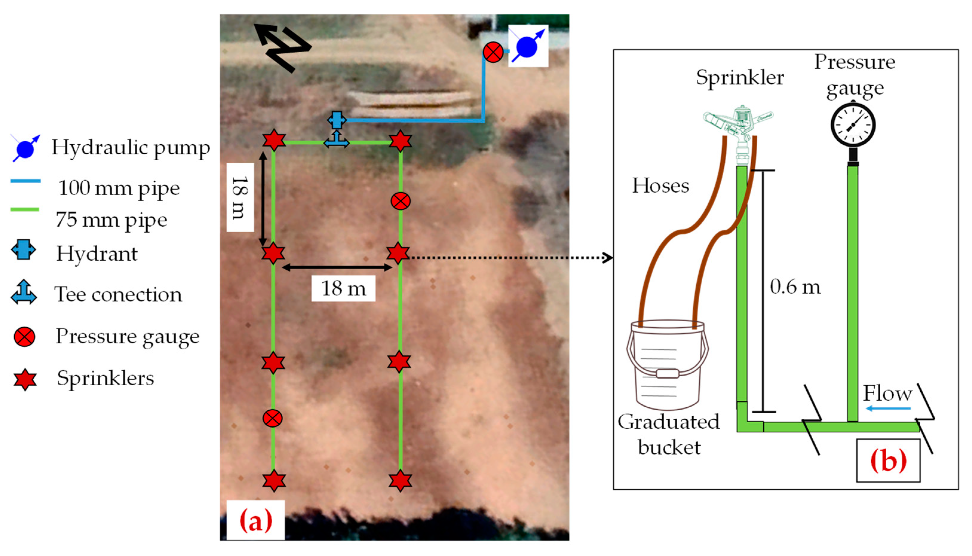
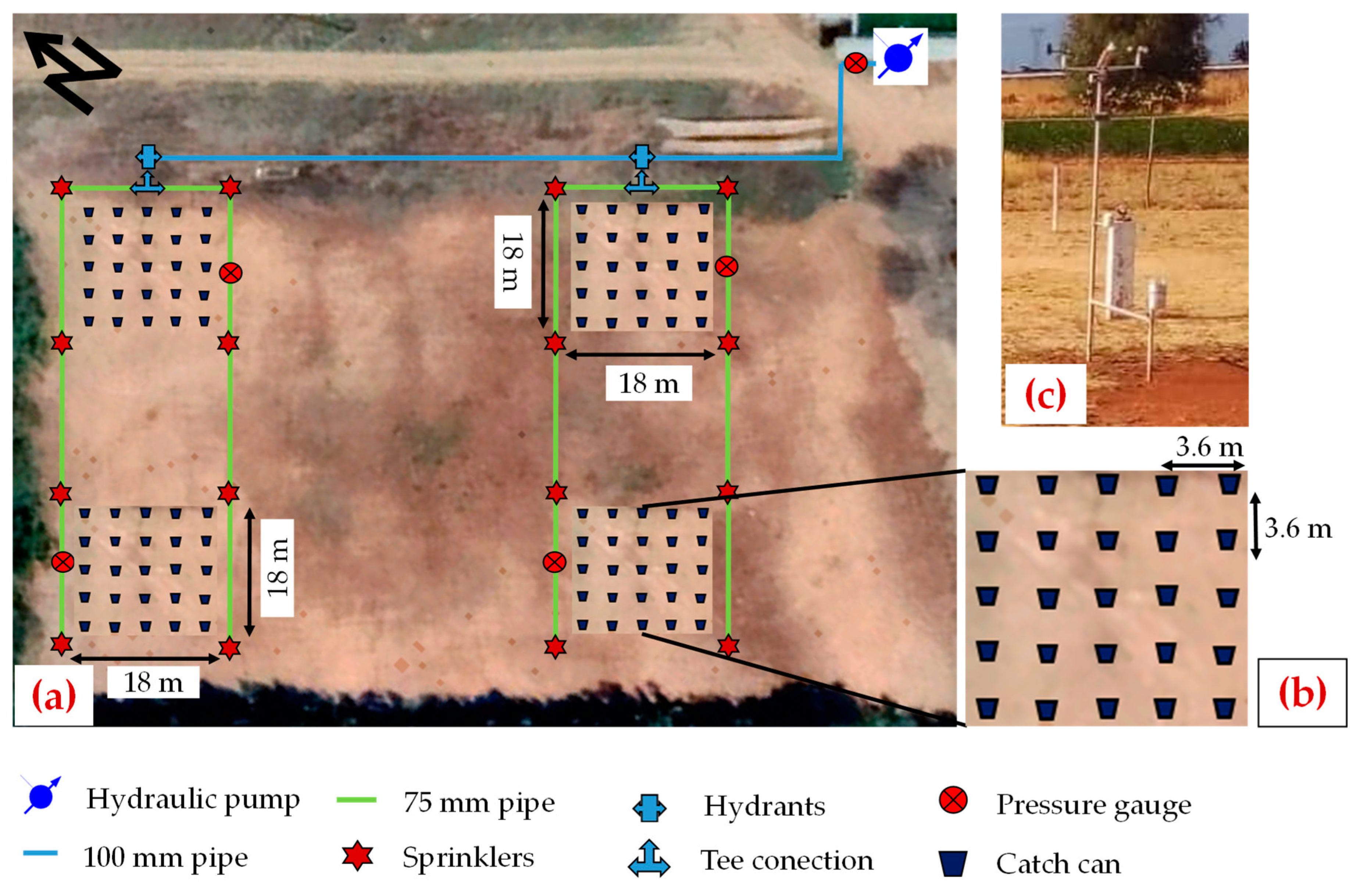
2.1. Field Solid-Set Experiments

The experiments were conducted at the facilities of the National Institute for Forestry, Agricultural and Livestock Research (INIFAP, Spanish acronym) in Calera de Victor Rosales, Zacatecas Mexico in 2021 [26]. The geographical coordinates are 23°36′ N latitude and 102°39′ W longitude, and an elevation of 2192 m above the soil level. The mean annual temperature is 14.6 °C with a mean annual rain of 416 mm.
Six different impact sprinklers with double nozzle, each commonly used in the region, were analyzed in this research for solid-set experiments (Table 1). The maximum and minimum main nozzle sizes were 5.56 mm and 4.37 mm, respectively, and the minimum auxiliary nozzle size was 2.38 mm. The operating pressures for the solid-set experiments were 200 kPa, 250 kPa and 300 kPa for each device. (Table 1) The ND 5035 and WR31 impact sprinklers were analyzed with two different main nozzle sizes each. The impact sprinklers ND 5035SD, SEN 4023-2 and WR 31 were made of plastic as their respective nozzles, and the rest were brass sprinklers with brass nozzles. The ND 5035 sprinkler had a plastic deflecting plate located in the straightening vane. This modification on the ND 5035 followed the Kincaid [27] developments and affects the main nozzle outlet jet, improving the radial application pattern and therefore increasing the CUC. With the same purpose, the SEN 4023 sprinkler had a plastic inner sheath before the main nozzle outlet. The wetted diameter (m) and the theoretical flow (L/h) were obtained for some sprinklers’ brands with available data at each operating pressure. The available wetted diameter for all sprinklers ranged between 22.8 m and 32.0 m depending on the sprinkler and the operating pressure. No information was provided by the manufacturer regarding the sprinkler height assessment for the wetter diameters except for the UR F30 sprinkler; also, theoretical flow is not available for some pressures. The theoretical flow available for all the sprinklers ranged from 1332 L/h to 2390 L/h with the maximum for the ND 5035 sprinkler with a 5.56 mm main nozzle size and 300 kPa pressure (Table 1).

2.2. Isolated Sprinkler Flow Measurements

Figure 1 shows the experimental setup for the flow measurements following the conventional volumetric method. The experiments were performed in the facilities of INIFAP [26]. The existing infrastructure was composed of a hydraulic pump, the 75 mm and 100 mm pipelines, the hydrants and tee connections and the riser pipes where sprinklers were located. The impact sprinklers with their respective nozzles were placed at the same time in a 75 mm pipeline (Figure 1a) in order to measure their respective flows in relation to the operating pressure. The eight sprinklers (two of them with the 5.56 mm main nozzles, one with 4.76 mm and the rest with 4.37 mm) were installed in two pipelines with a 18 m × 18 m square configuration (Figure 1a). Sixteen hosepipes of 1 m length each were installed in pairs in both nozzles of each sprinkler for collecting the application volume in a graduated bucket with 20 L maximum capacity. Three water measurements were performed for each sprinkler at each pressure. The measurements were performed in one sprinkler at the time and a chronometer was used for measuring the bucket-filling time. The system operated between 27 and 56 s for all the application volume experiments till the catch can were filled. The operating pressure was supervised in each sprinkler test with a glycerin pressure gauge at the hydraulic pump and with two more installed in the two pipelines (Figure 1b). The flow (L/h) vs pressure (kPa) curves were obtained at more pressures with respect to those reported in the solid-set experiments for a full sprinkler characterization. They ranged from 200 kPa to 380 kPa with 50 kPa intervals. A large sprinkler characterization helped to compare the data reported by the sprinkler brands. Also, the isolated experiments provided information not given by the brands, which provided some information only about the sprinkler performance mainly at 300 kPa and just a few demonstrate sprinkler features at 200 kPa, but no information is given at 250 kPa except for the SEN 4023 and WR 32 sprinklers. Low-pressure SSSI systems have been implemented [24,27,28,29] as a new irrigation design in order to reduce the energy use without affecting the crop yield, maintaining the irrigation performance and the current spacing.

2.3. Irrigation Performance Measurements

The experiments were performed in a plot of approximately 0.5 hectares (the same as the flow measurements’ experiments in the INIFAP plot). This was configured with two hydrants, one for each pipeline pair (Figure 2). The water applications’ pattern differs from one sprinkler to another even with the same operating pressures or nozzle sizes. The material and accessories varied for different sprinklers besides their performance at different meteorological conditions. The water application patterns were measured in four subplots at the same time with a square sprinkler layout configuration of 18 m × 18 m between the pipelines and the sprinklers (Figure 2a). The four subplots were separated by 18 m in a vertical direction and 30 m in a horizontal direction in order to measure the water application without the interference of other subplots’ irrigation. The predominant wind direction was northeast. The sprinklers were 360° full circle rotating.
The operating pressure was supervised in all the tests with a glycerin pressure gauge. Four sprinklers of the same type were installed in each of the four subplots. At the same time, 16 sprinklers were operated in the plot (Figure 2a). The irrigation system operated with one pressure till the number of proposed measurements were achieved. The number of tests for each sprinkler depended on reaching the water application patterns with three different wind velocities with ranges: ≤2 m/s, 2 m/s to 4 m/s and greater than 4 m/s. The experiments were performed between 31 July and 15 August 2021 from 7:30 a.m. to 5:00 p.m. in order to obtain a full characterization along the day. The system was operated for 2 h at each irrigation event. The sprinklers were installed at a height of 0.6 m AGL.
The water application distribution was assessed with a 25 catch-can grid in each subplot distributed homogeneously on the area of 324 m2 with 3.6 m × 3.6 m between the sprinklers and the pipelines, respectively, (Figure 2b) following the methodology of Playán et al. [23]. The catch-can grids remained in each subplot during all the experiments. The irrigation events lasted for two hours. The catch-can water depth was measured using a cylinder graduated in milliliters in all subplots. Therefore, the volume in milliliters of each catch can was converted to irrigation depth in millimeters per hour considering the catch-can influence area (3.6 m × 3.6 m) and the irrigation time (2 h). The pluviometers used are made of plastic with 0.11 m upper diameter, 0.09 m lower diameter, 0.07 m height and 0.5 L maximum capacity. The catch cans were located at ground level, leaving a 0.51 m height from the pluviometer mouth to the sprinkler nozzle, the previous catch-can features were consistent with ISO 15886-3 [13]. The irrigation depth obtained per experiment was used to determinate the Distribution Uniformity (DU, %) [15] (Equation (1)) and Christiansen’s Uniformity Coefficient (CUC, %) [16] (Equation (2)).
DU = ( Z l q Z a v g ) × 100
where Zlq is the mean lowest one quarter irrigation depth in the catch can grid (mm/h) and Zavg is the mean irrigation depth accumulated in all the catch cans (mm/h).
CUC = ( 1 i = 1 n | Z i Z a v g | n x   Z a v g ) × 100
where Zi is the applied irrigation depth measured in each of the 25 catch cans within the grid (mm/h) and n is the total number of catch cans.
Moreover, WDEL were also computed as the difference between the applied irrigation depth and the collected irrigation depth in the catch can grid according to Playán et al. [23] for each sprinkler type, nozzle size, operating pressure and wind velocity scenario. The data of each irrigation event (sprinkler test, date, total amount of water applied in the catch can, operating pressure, irrigation collected within every catch can, irrigation time, and meteorological variables) were sorted in individual spreadsheets classifying the experiments according to their wind velocity (downloaded from an agrometeorological station near the plot) for all sprinklers. Spatial variability in water distribution patterns was assessed using contour line maps made with the ®SURFER software (Golden Software Inc., Golden, CO, USA) for each irrigation event.
An automated agrometeorological station controlled by the Agroclimatic Monitoring Network of INIFAP [26] was already located at 200 m from the plot (Figure 2c). The following variables were downloaded from INIFAP rainfall (mm), relative humidity (%), temperature (°C), wind direction (0–360°) and wind velocity (m/s). The variables were measured at 2 m height above ground level (AGL) every minute and the values were reported as averages every 15 min.

2.4. Data Analysis

WDEL and the CUC were related with the meteorological variables measured for each test type in order to obtain models through multiple linear regression analysis. Analysis of variances was also performed in order to detect significant differences for both models (WDEL and CUC) at p = 0.05 confidence level. Several research works of SSSI [24,30,31,32,33,34,35,36,37,38,39,40,41,42] were analyzed for assessing WDEL and CUC (Table 2). The criteria for choosing the models were the measured variables of this study. The vapor pressure deficit (es − ea) was not measured in this research but it was obtained according to Trimmer [30] (Equation (3)). The obtained es − ea was used for adjusting the WDEL models of Trimmer [30], Montero [31], Tarjuelo [32], Maroufpoor [40] and the model of this research.
e s e a = 0.61   e x p ( 17.27   T T + 237.3 ) ( 1 R H 100 )
where T is the air temperature (°C) and RH is the relative humidity (%).
The CUC models of Sánchez et al. [37] and Stambouli et al. [38] reported in their publications were adjusted to our experimental data in order to assess the best model performance. The CUC models of Robles et al. [24], Playán et al. [28], Nin [33], Saraiva et al. [34] and Ouazaa et al. [39] reported in Table 2, were obtained from a multiple linear regression analysis using the full experimental data reported in their publications. In the same way, the WDEL model of Saraiva et al. [34] was obtained. Multiple linear regression analysis was performed with the experimental data in order to obtain WDEL and CUC models. Analysis of variance for each model and Fisher’s least significant difference test (LSD) between models at p = 0.05 confidence level were performed. In order to assess the predictive ability of both models types, WDEL and CUC estimated with the author´s models (Table 1) were compared with the models of this research in terms of the coefficient of determination (R2).

3. Results and Discussion

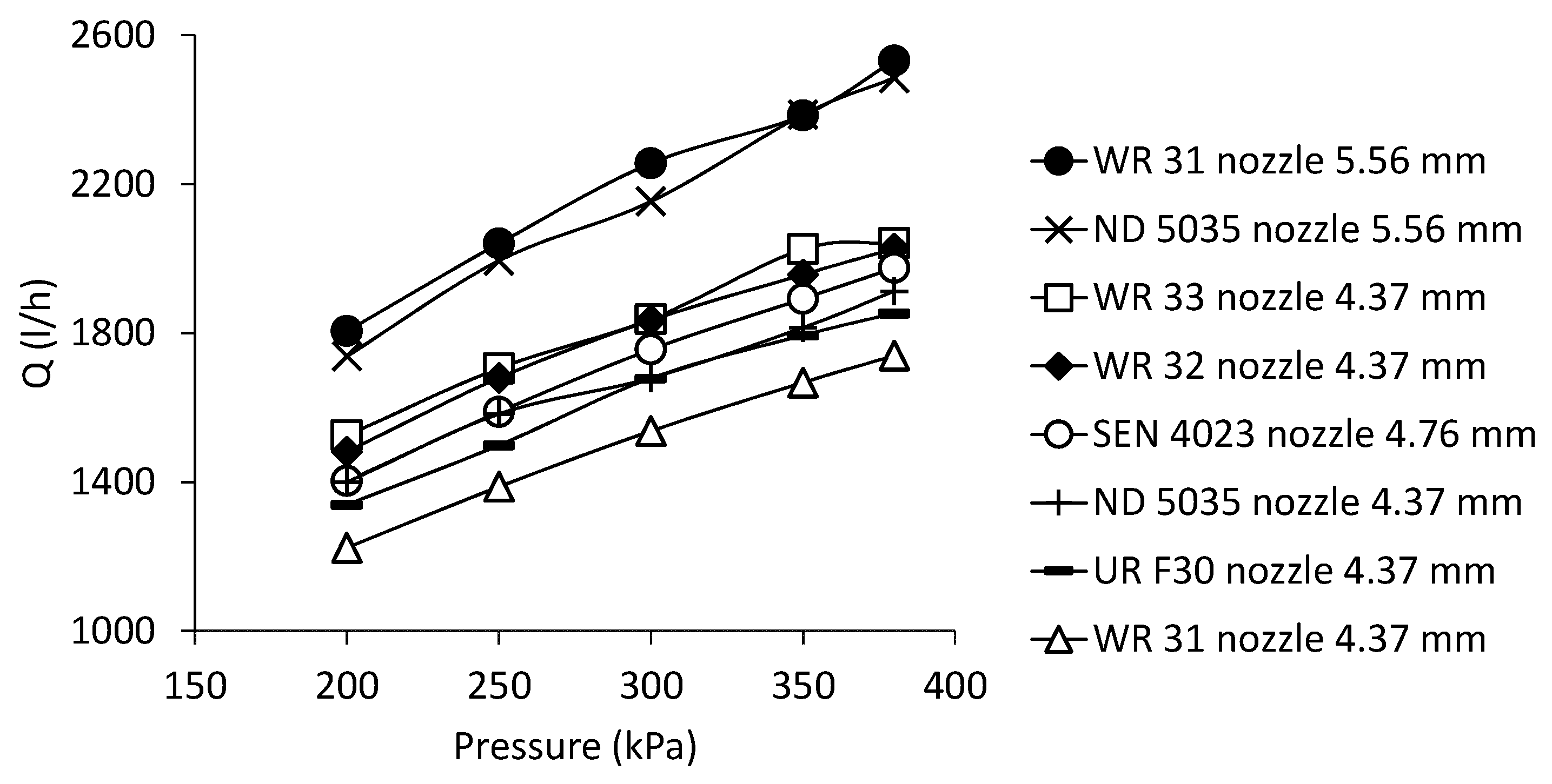
3.1. Sprinklers Flow

A total of 120 flow measurements were performed for the 8 impact sprinklers at the 5 pressures (200, 250, 300, 350 and 380 kPa) with their respective nozzles (Figure 3).
In general, analyzing the maximum sprinkler flows, the WR 31 impact sprinkler with 5.56 mm main nozzle size presented the highest flow with 2532 L/h at 380 kPa. In comparison with the ND 5035 sprinkler, the WR31 got an average of 3% highest flow with the 5.56 mm main nozzle for all the pressures with a standard deviation of 52 L/h. This difference was because the ND 5035 impact sprinkler was equipped with a smaller auxiliary nozzle (2.50 mm) compared with the WR 31 sprinkler (3.18 mm). By contrast, the lowest flow was obtained for the WR 31 with the 4.37 mm main nozzle diameter for all the pressures with a minimum value of 1224 L/h. The differences in the measured flows with respect to the brands were lower than 5% for the sprinklers with the main nozzles smaller than 5 mm; these differences increased (≤9%) with the other nozzle diameters and could be explained by experimental error.

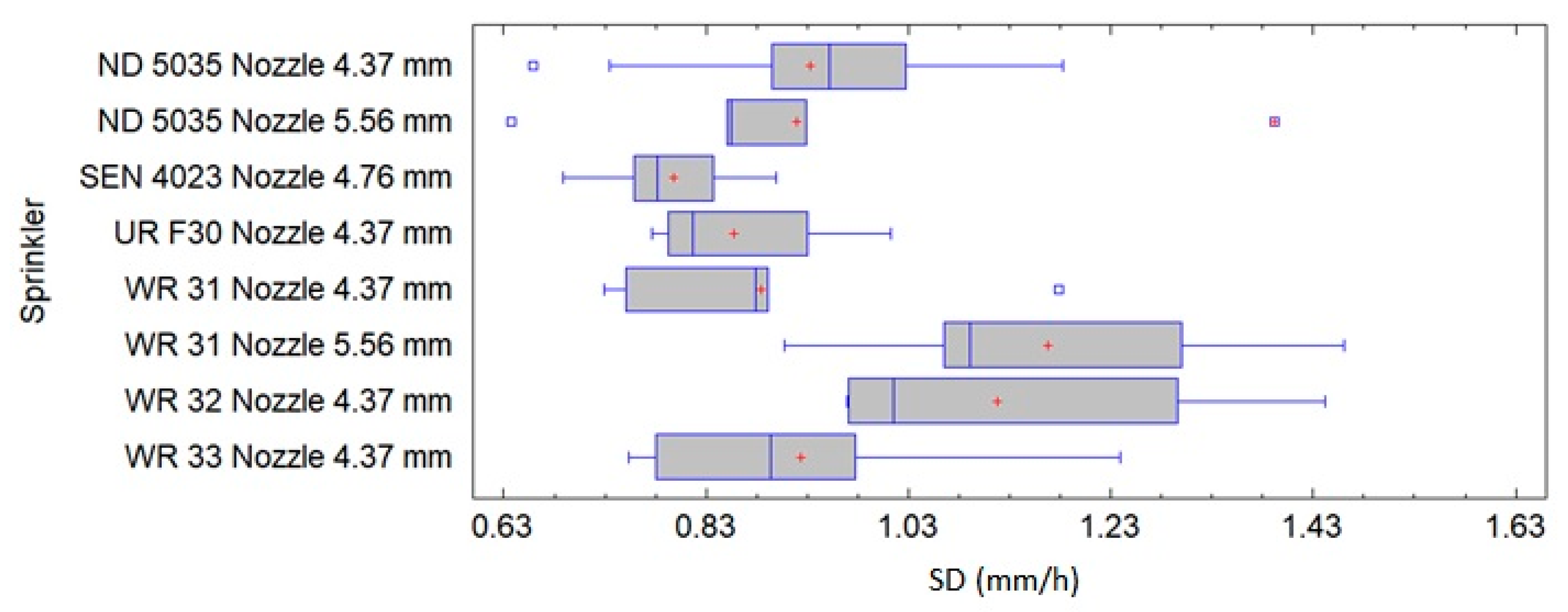
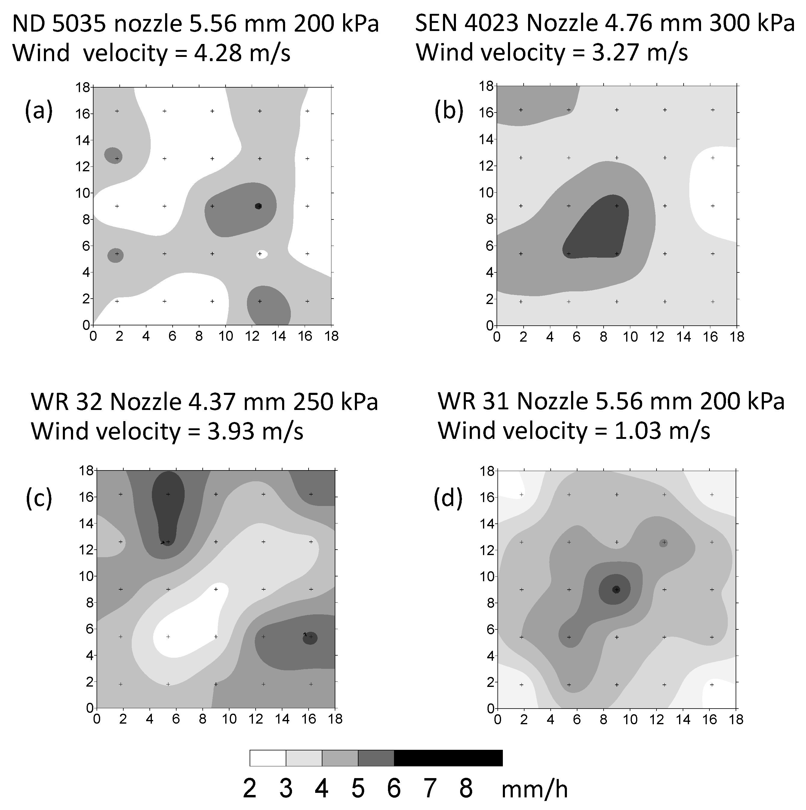
3.2. Sprinklers’ Water Distribution Patterns

The spatial distribution variability was assessed in terms of the standard deviations (SD) of the irrigation water depth (mm/h) collected within each solid-set experiment for each sprinkler type with the data collected from the 25 catch cans and was summarized as a box-whisker plot in Figure 4. The total number of solid-set experiments was 60. The number of trials per sprinkler showed in Figure 4 could be seen in the Appendix A and they varied between 6 and 9 tests per sprinkler.
Moreover, the significant differences found were analyzed using the Fisher´s LSD test at p = 0.05. The effect of the pressure on the water distribution SD was also analyzed with ANOVA using the SD as a dependent variable.
After the LSD test, the impact sprinklers of WR 31 with a main nozzle of 5.56 mm and WR 32 with a main nozzle of 4.37 mm presented the largest variability and were significantly different compared with the rest of the sprinkler types at p = 0.05 (Figure 4). There were no significant differences between the SD of the water distribution and any of the operating pressures at p = 0.05.
In general, the impact sprinklers ND 5035 and the SEN 4023 sprinklers presented the smallest spatial variations of the water distribution within the frames. These variations did not depend on the operating pressure or the wind velocity. In general, the sprinklers showed an average application rate of 4.92 mm/h with a mean standard deviation of 0.85 mm/h. Figure 5 shows examples of solid-set experiments with low and high water distribution variability for different wind velocities. Wind velocity is the most important variable on sprinkler irrigation performance (WDEL, CUC or DU). The Figure 5a,b are two experiments of both sprinkler types (ND 5035 and SEN 4023) with different wind velocities. On the other hand, Figure 5c,d showed two experiments which presented the highest water distribution variability for the WR 32 and WR 31 sprinklers, respectively. In general terms for both sprinkler types, a mean irrigation of 5.26 mm/h with a mean standard deviation of 1.15 mm/h values were observed.

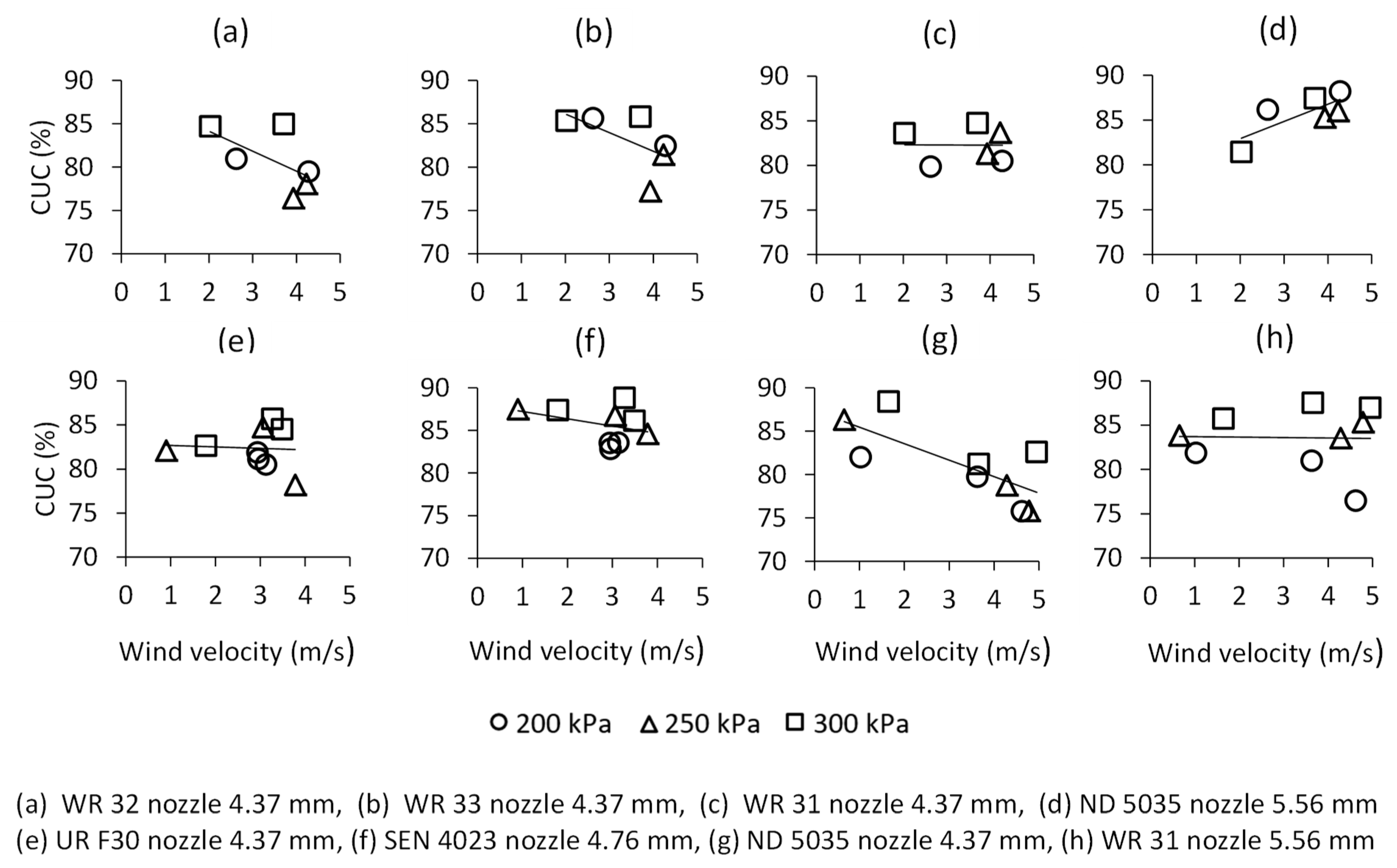
3.3. Irrigation Performance Based on CUC

A total of 60 experimental tests were performed for measuring the water application depth through 1500 catch-can measures to compute the Christiansen uniformity coefficient (CUC) and the distribution uniformity (DU). The data were captured in spreadsheets and the tests were classified for sprinkler type, wind velocity and operating pressure. Between 2 and 3 tests were performed for impact sprinklers at each pressure covering the 3 wind velocity scenarios.
In order to assess the irrigation performance in terms of CUC, Figure 6 shows the uniformity computed for sprinkler type related to wind velocity for all tests. In general, the low variability of the water distribution of the sprinklers ND 5035 (main nozzle of 5.56 mm) and the SEN 4023 (main nozzle of 4.76 mm) caused the highest average uniformities for the 60 solid-set experiments (Figure 6d,f, respectively). The mean uniformity for these sprinklers reached 86% without significant differences between sprinklers after a LSD test at p = 0.05. The differences between the ND 5035 and SEN 4023 sprinkler reached 2% of CUC standard deviation with wind velocities between 0.9 m/s and 4.5 m/s. On the contrary, the impact sprinkler WR 32 with the main nozzle of 4.37 mm presented the lowest uniformity values with a mean of 80% and a higher variation of 4% SD as was expected by its water distribution (Figure 6a) for a maximum wind velocity of 4.3 m/s. Despite this low uniformity value, it could be considered as acceptable since it is close to the 84% recommended by Keller and Bliesner [12].
From Figure 6, the sprinklers WR 31, WR 32 and WR 33 produced a CUC average of 79% at 200 kPa and the ND 5035 and SEN 4023 sprinklers obtained an 85% CUC average at the same pressure. Considering 200 kPa instead the standard 300 kPa meant decreasing by a third the operating pressure of the SSSI and, therefore, the energy requirements of the irrigation systems as reported by Robles et al. [24,29]. Mean CUC values could be observed in Appendix A for the 60 experiments.
Robles et al. [24] used the same ND 5035 impact sprinkler in their experiments with a smaller main nozzle diameter of 5.16 mm, pressures of 200 kPa and 300 kPa and wind velocities between 1 m/s and 7 m/s (11 experiments in total). Considering an umbral of 4.5 m/s wind velocity for the same ND 5035 sprinkler, the authors found a mean value of 85% in CUC (8 experiments) and more variability (9% of SD) in comparison with our research work with 86% and 2% SD (6 experiments). The CUC values of Robles et al. [24] ranged from 67% to 94% for this sprinkler type. Their differences could be explained for the sprinkler height at 2 m since the drops are more affected by wind velocity and direction. In this research work, mean values of 86% were found for the sprinkler ND 5035 installed at a height of 0.6 m with wind velocities lower than 4.5 m/s. It was noticeable that CUC was above the recommended value (84%), even with high wind velocities. This could possibly be attributed to the sprinkler height. Sprinkler height depends on the plants’ height so this research focused on a technical analysis for SSSI for crops with small canopy growth. In comparison with Robles et al. [24], in this research no CUC values of 90% or higher were found. This was the case even at low wind velocities, possibly because of the sprinkler height that could influence/limit the horizontal range of the drops within the solid-set spacing and therefore affect the overlapping between the water application patterns of the sprinklers as had been noticed by [29,33,37,43] with different sprinkler heights. In order to achieve higher uniformities, further research is need changing the distance between pipelines and/or between sprinklers.
Moreover, a positive correlation of the CUC related to the wind velocity was observed for the ND 5035 impact sprinkler with the main nozzle of 5.56 mm with all pressures analyzed. This meant that the CUC increases with wind velocity up to a certain limit. This was also observed by Nin [33] in his experiments with an Agros 35 impact sprinkler operating at 300 kPa pressure with a 5.2 mm main nozzle. The author separated linear regressions of CUC vs. wind velocity below and above 2 m/s, up to 6 m/s. He obtained a highest CUC value of 81% for low wind velocity, similar to those of this study. The pattern of the ND 5035 impact sprinkler could possibly be explained by the modifications made to the sprinkler arm next to the main nozzle (deflecting plate attached) and due to the large main nozzle size compensating the CUC. The possible explanation for the results of Nin [33] could be the main nozzle size and a vane located inside the sprinkler where the larger nozzle is installed. The deflecting plate attached to the arm improves the radial application pattern of the sprinklers, modifying into a triangular profile [27,29,33,43] that increase the CUC. The effect of using large nozzle sizes with a straightening vane inside the sprinkler, particularly for the highest pressures, could reduce the drops drift and increase the CUC [33]. None of the other sprinklers tested had similar features to these. The impact sprinkler WR 31 with the main nozzle size of 5. 56 mm did not have any extra accessories, worsening the uniformity at low pressures but not for the conventional 300 kPa. For this WR 31 sprinkler with the largest nozzle, the CUC values ranged between 77% and 88% with a SD of 4% (Figure 6h).
Regarding the sprinkler WR 31 with the main nozzle size of 4.37 mm (Figure 6c), the behavior of CUC with respect to the wind velocity was almost constant considering all wind scenarios. For this sprinkler and nozzle size, the CUC increased with the pressure and it was maintained between 80% and 84% with a mean value of 82% and a SD of 2%. A constant correlation was also observed for the UR F30 sprinkler with CUC values higher than 80% in all test with the exception of one test at 250 kPa with the highest wind velocity (Figure 6e). The rest of the sprinklers relationships showed in the Figure 6a,b,e,f,g presented a negative tendency relating the CUC vs. the wind velocity for the differences mentioned above in this section. All experimental data could be seen in the Appendix A.
Wind direction usually presented large variability (i.e from 0–360°) during the irrigation as long as it lasted. Different wind direction modifies the water distribution inside an isolated subplot (i.e., 18 m × 18 m as Figure 5) leaving some sections less or more irrigated than others. In a real plot with a crop, there are no empty subplots between sprinklers that would imply a smaller sowing area. The irrigation inside a subplot could therefore be influenced with the irrigation water of other subplots, particularly high wind velocities. Analyzing an individual subplot in a plot, these differences in water distribution could be compensated with the other subplots’ irrigation compensating the overall plot water distribution and therefore the uniformity. Considering a hypothetical case of a constant wind direction during a whole crop season, this could produce deficiencies in crop growth, reducing yields in some sections of the plot without considering soil problems, agronomic variables or water quality. Nevertheless, no water input was observed in our experimental evaluations from one subplot to another due to the spacing as shown in Figure 2. Moreover, the trials were performed according to the international standards and common practices worldwide for the SSSI [12,13,14,15,16,17,18].
With respect to the DU of the experiments, similar patterns of the CUC were observed in DU; the highest DU mean values were obtained for the ND 5035 and the SEN 4023 sprinkler with an average of 80% for both, and the minimum average was for the WR 32 sprinkler with 72% (Appendix A).

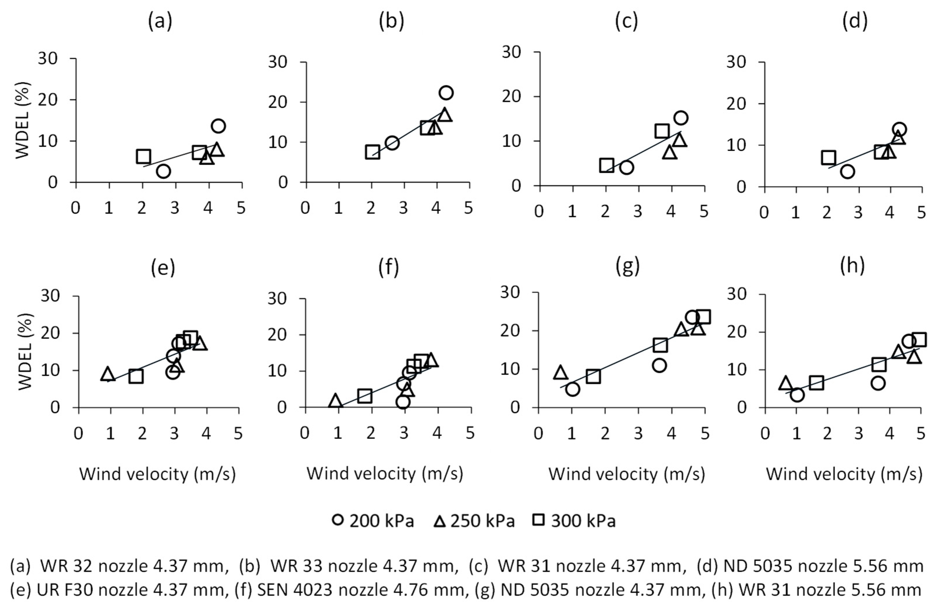
3.4. Wind Drift and Evaporation Losses

For all the 60 solid-set experiments the following ranges of the main meteorological variables were found: between 0.5 m/s and 6 m/s of wind velocity, from 14 °C to 25 °C for air temperature and between 40% and 85% of relative humidity. The mean WDEL obtained ranged from 7.16% to 15.3% for all experiments (Appendix A). The predominant wind direction in all the experiments was the east with variations from north to south in 75% of the irrigation time. The irrigation infrastructure already installed in the INIFAP [26] field followed the plot geometry. The catch-can grids were installed following the pipelines’ orientation in each subplot. In the same way as with the CUC, no water drops were observed to be drifting from one subplot to another in our experiments. According to the Table 1, the incomplete theoretical data of the wetted diameter showed a maximum value of 32 m for the highest pressure. Further research is needed in order to measure the real wetted diameter for all the sprinklers, pressures, and different wind velocities analyzed at a given sprinkler height. The wetted diameter is commonly obtained through measurements of the radial application patterns on isolated sprinklers [16,28,29,37,38,39,44].
Figure 7 shows WDEL for each sprinkler type at their experimental wind velocities. The largest variability and the highest values of WDEL were observed for the ND 5035 impact sprinkler with a nozzle diameter of 4.37 mm (Figure 7g), For this sprinkler WDEL reached values higher than 20% at wind velocities around 4 m/s. Significant differences on WDEL were found between the WDEL of the ND 5035 (4.37 mm main nozzle) and four different sprinklers (ND 5035–5.56 mm nozzle, Sen 4023, WR 31–4.73 mm nozzle and WR 32).
The lowest WDEL average was obtained for the WR 32 sprinkler with the 4.37 main nozzle size and the SEN 4023 sprinkler, considering all the experiments with 7.3% and 7.2%, respectively. In analyzing the WR 32 and WR 31 (5.56 mm main nozzle) sprinklers, it had been previously discussed that the sprinklers presented the largest variability on water distribution mainly for low pressures. These previously generated low CUC values for the same pressures (79%) but an 86% mean CUC for both sprinklers at 300 kPa. Regarding WDEL for the same sprinkles, mean values of 10% were found for both low and standard pressures. In general, it was noticeable that WDEL were larger for the WR31 (5.56 mm nozzle) for wind velocity ≥4 m/s (Figure 7h). It was not expected that WR 31 and WR 32 generated the largest WDEL at 200 kPa (Figure 7a,h) mainly at high wind velocities. From the previous discussions it seemed that WR 31 and the WR 32 (5.56 mm nozzle) were not suitable for low pressures because of their irrigation performance: a large variability in water distribution; low CUC values; and high WDEL. Nevertheless, it seems that the sprinklers at 300 kPa produced proper indexes at wind velocities lower than 4 m/s. Nevertheless, more field experiments are needed for these sprinklers in order to confirm the previous assumptions.
The impact sprinklers ND 5035 with a main nozzle of 5.56 mm and SEN 4023 obtained the highest CUC values (86%) with 2% SD and a lower variation in water distribution (mean SD of 0.85 mm/h). The sprinklers also produced the lowest values of losses in evaporation and drift with an average of 9% (Figure 7d) and 7% (Figure 7f). Moreover, on analyzing the effect of WDEL on the different sprinkle types for all the pressures and wind velocity scenarios, no significant differences were found between the WDEL of the ND 5035 sprinkler (5.76 mm nozzle size) in comparison with the WDEL of all the sprinklers. But significant differences were found between this sprinkler with respect to the sprinkler ND 5035 (4.37 mm main nozzle size), after a Fisher´s LSD test at 95% confidence level. No significant differences were found between the sprinklers WR 32 (Figure 7a), WR 31 (4.37 mm nozzle size) (Figure 7c) and ND 5035 (5.56 mm nozzle size) (Figure 7d) for the WDEL, reaching an average of 8.40% for all the experiments.
No significant differences were observed for WDEL between the WR 33 (Figure 7b) and the UR F30 (Figure 7e) sprinklers with an average of 14% for both after an LSD test at p = 0.05 for all experimental scenarios. Full experimental data of WDEL can be observed in Appendix A.
The computed values of the experimental WDEL showed in Figure 7 were related to the meteorological variables of the 60 solid-set tests in order to obtain a general predictive model based on a multiple linear regression, as follows in Equation (4):
WDEL = 2.93435 E d + 1.5234 U 0.199672 R H 0.0855265 T + 0.01176 P + 29.2861
where WDEL are expressed in percentage, Ed is the equivalent diameter (mm), considering both nozzle sizes according to Robles et al. [24]. U is the wind velocity (m/s); RH is the relative humidity (%); T is the air temperature (°C); and P is the operating pressure (kPa).
This model as Equation (5) explains 56% (determination coefficient, R2) of the variability of the WDEL as measured. In other sense, the wind velocity was used as the independent variable for predicting the experimental WDEL. The variable by itself explained most of WDEL variability with 44.96% R2 as it had been noticed by a number of researchers works [22,23,24,36,42]. In agreement with Robles et al. [24] Equation (5) also explains the physics behind the losses due to the evaporation and drift that increase with the wind velocity and the pressure, and decrease with the nozzle diameter, the relative humidity and the air temperature being the first and most important, indicating that the main losses are due to the drops’ drift.
The WDEL equations proposed by the authors in Table 2 adjusted the experimental variables measured in this research in order to assess their predictive capability in relation to the experimental data. The measured WDEL of this research was then related to estimates by the authors as shown in Figure 8. In general, WDEL presented significant differences with most of the equations except for the models of Playán et al. [23], Montero [31] and Tarjuelo et al. [32]. The coefficient of determination (R2) indicates low correlations between measured and estimated losses with a maximum value of 0.58 for the relationship of Trimmer [30] but overestimates the WDEL measured up to 50%. In Figure 8, the relationships more adjusted to the 1:1 line were obtained for Montero [31] (R2 = 0.50), Tarjuelo et al. [32] (R2 = 0.51), Playán et al. [23] (R2 = 0.47), Playán et al. [28] (R2 = 0.49), Sánchez et al. [37] (R2 = 0.48), Stambouli et al. [38] (R2 = 0.47) and Robles et al. [24] (R2 = 0.50). The large variability and differences of WDEL from one model to another indicates a dependency on different factors such as: the climatic variables depending the irrigation time (day or night); the solid-set configuration; the sprinkler type and its accessories and the nozzle diameters. The multiple linear regression obtained from the experimental data from Saraiva et al. [34] underestimated WDEL measured with values lower than 4% for all experiments of this work. The experimental conditions of Saraiva et al. [34] were as follows: sprinkler spacing of 12 m × 12 m; main nozzle size of 3.5 mm and 2.5 mm auxiliary nozzle; a total number of 12 experiments for pressures ranged between 200 kPa and 350 kPa every 50 kPa and similar meteorological variables measured compared with this research work. The experimental conditions of Playán et al. [23] were the 85 experiments, the sprinkler spacing of 15 m × 15 m, the sprinkler height at 2 m, one sprinkler type tested (VYR70) and trials with two nozzle sprinklers (4.4 mm and 2.4 mm). It is noticeable that our WDEL and those of Playán et al. [23] were obtained with various experiments and the experiment of Saraiva [34] was obtained with 12 observations. Also, the predictive WDEL model generated from Saraiva et al. [34] poorly represents their CUC experimental data with 34% of R2 given that the model of Playán [23] reached an R2 of 80%. Robles et al. [24] (Figure 8k) showed higher WDEL estimated with their predicted model compared with the observed values, probably due to their measurements at heights above 2 m, increasing WDEL.

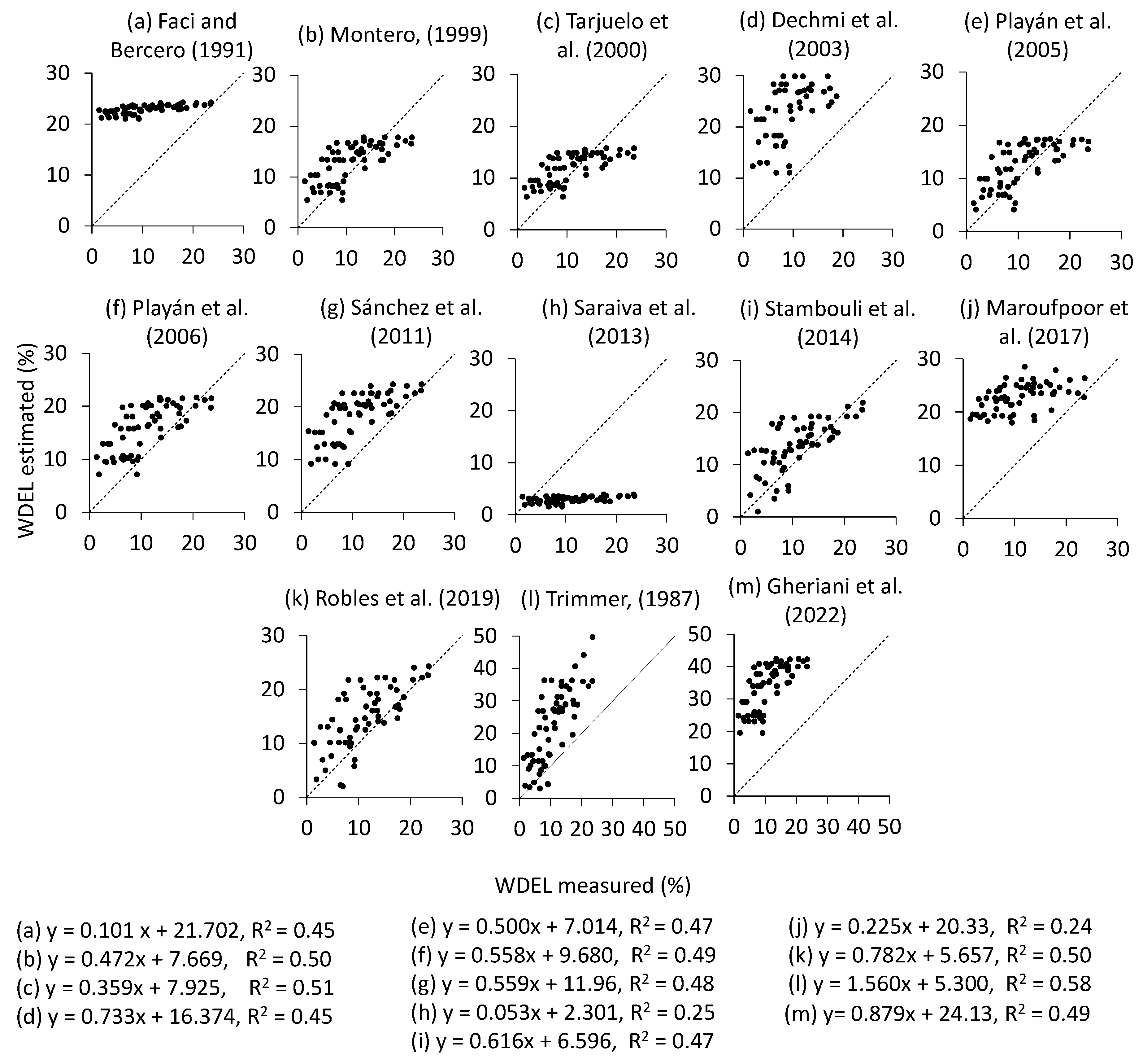
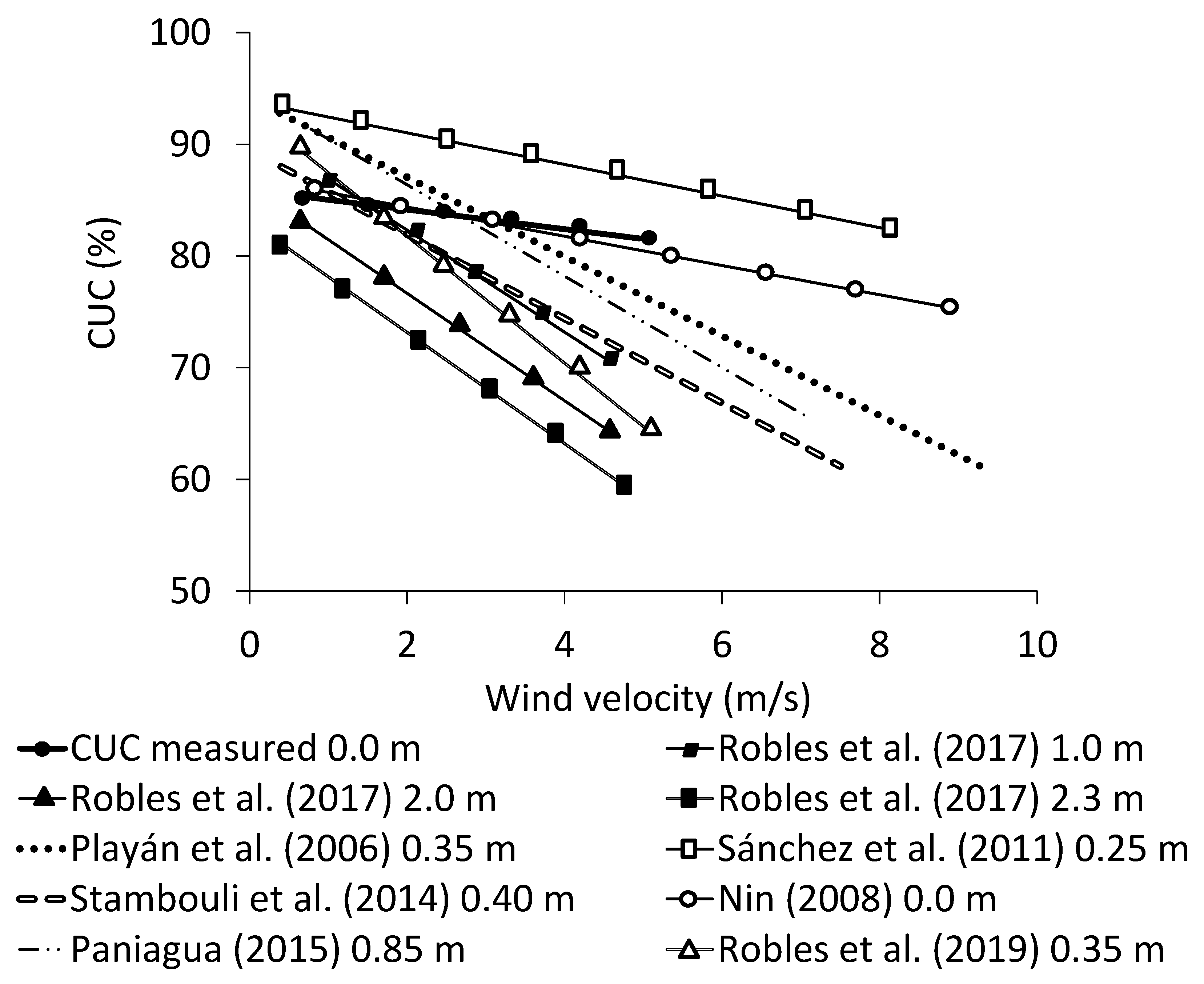
3.5. Comparison between CUC Models

The CUC models reported in Table 2 were adjusted to our experimental data (nozzle diameters, wind velocity and pressure) and were then related to the experimental CUC values through linear regressions for the 60 solid-set experiments performed. Correlation equations are shown for each comparison with their respective determination coefficient (R2) (Figure 8).
The multiple linear regression obtained for CUC measured was obtained as Equation (5). After analyzing the parameters involved in the irrigations, the predictive CUC model selected was defined with the objective function of maximizing R2 with respect to the experimental data. Equation (5) represents the CUC variability in 40% (R2) with significant differences between the independent variables. The variables selected for CUC regression were the equivalent of diameter–Ed, according to Robles et al. [24], wind velocity–U and operating pressure–P. The equations obtained from the research works of Sánchez et al. [37] and Stambouli et al. [38] were also used as independent variables for the wind velocity and the pressure but not the nozzle diameter.
In general, from the CUC experimental data it could be noticed that uniformity as Equation (5) decreases with the wind velocity (this variable being the most important affecting the CUC) and increases with the operating pressure (although with low representation in the model). Considering the models reported in Table 2 and Equation (5), the effects of the nozzle diameters on the dependent variable (CUC) are not clear but they are representative in the models. In the Playán et al. [28] model, the CUC increases with the nozzle size as much as Equation (5) but the opposite is observed with the rest of the models in Table 2 (Robles et al. [24] and Nin [33]).
CUC = 2.61365 E d 0.82475 U + 0.03456 P + 65.9685
The CUC models from the authors reported in Table 2 (Robles et al. [24]; Playán et al. [28], Nin [33], Saraiva et al. [34], Sánchez et al. [37], Stambouli et al. [38] and Ouazaa et al. [39]) were assessed with our experimental data and were related to the CUC measured in this study (Figure 9). In general, both positive and poor correlations were observed in all cases, with the R2 value < 0.2 obtained for the correlation of Sánchez et al. [37] (Figure 9c). The closest relationships to the 1:1 line were Robles et al. [24], Playán et al. [28], Saraiva et al. [34] and Sánchez et al. [37] with poor correlations (R2) of 0.08, 0.18, 0.05 and 0.21, respectively. The other comparisons presented large deviations from the 1:1 line and also low R2. These poor correlations to our CUC data could be attributed to different issues: (1) sprinkler height (0.6 m in this work and ≥2 m in the other references); (2) the number of experiments of each research work, as previously discussed on the WDEL models; (3) the experimental conditions (wind velocity ranges, sprinkler spacing, nozzle sizes, pressures). The CUC averages from Playán et al. [28], Saraiva et al. [34] and Sánchez et al. [37] were not statistically significant with respect to the CUC measured at 95% confidence level after a Fisher´s LSD procedure. The minimum CUC values were obtained with the model of Ouazaa et al. [39] related to our data (Figure 9f) with 61% and was also the model that produced the largest CUC variability (8% of standard deviation).

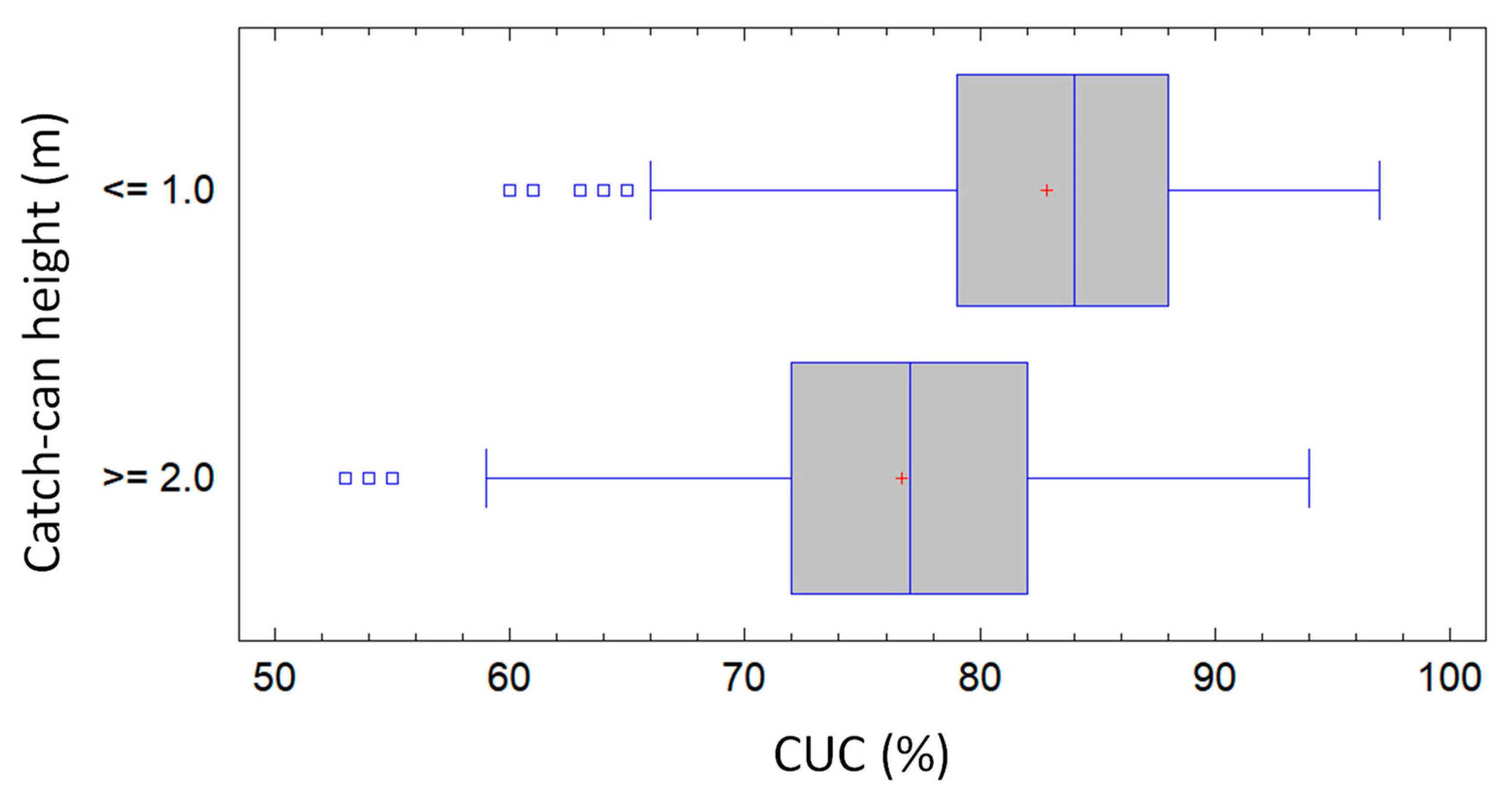
3.6. Influence of the Catch-Can Height on Irrigation Performance

One important factor to take into consideration in the irrigation performance is to analyze the different uniformities in the catch-can height. Figure 10 shows the relationships between Christiansen´s uniformity coefficient and the experimental wind velocity from a number of research works on SSSI [24,28,29,33,37,38,39,40,41,42,44] for different catch-can heights.
Figure 10 reported the CUC measurements of Robles et al. [29] on two impact sprinklers working at 200 kPa and one more at 300 kPa with the sprinklers located at 2.5 m AGL. These CUC were measured at different catch-can heights: 1.0 m (15 experiments), 2.0 m (39 experiments) and 2.3 m (54 experiments).
Moreover, in Figure 10, more research works of SSSI were included: (1) 41 experiments performed by Playán et al. [28] with evaluations at 2.0 m for the sprinkler height and 0.35 m AGL and the catch-can height at 200 kPa, 300 kPa and 400 kPa; (2) 55 experiments from Sánchez et al. [37] with 2.0 m the sprinkler height and 0.25 m and the catch-can height at 240 kPa, 320 kPa and 420 kPa; (3) 49 experiments from Stambouli et al. [38] with the sprinkler height at 2.0 m AGL and the catch-can height at 0.40 m AGL at 200 kPa, 300 kPa and 400 kPa; (4) 11 experiments performed by Paniagua [44] with the sprinkler height at 2.45 m AGL and the catch can at a height of 0.85 m AGL at 200 kPa and 300 kPa; (5) 11 experiments performed by Robles et al. [24] with the sprinkler height at 2.0 m and the catch-can height at 0.35 m AGL at 200 kPa and 300 kPa.
Figure 10 also includes the 61 experiments of Nin [33] on impact sprinklers at pressures from 220 kPa to 450 kPa, performed with the sprinkler height at 2.0 m and the catch can located at the soil level. The 60 experiments performed in this study are also shown in Figure 10, performed at 0.60 m for the sprinkler height, the catch can at the soil level and at 200 kPa, 250 kPa and 300 kPa. A total of 396 CUC experiments were related to wind velocities in Figure 10 similar to the operating pressure for the previous research works in respect of the catch-can heights.
Table 3 summarized the features of each research work included in the Figure 10. The effective height in m was obtained as the difference between the sprinkler height and the catch-can height and was reported for all the research works in Table 3. The effective height of ≤1.5 m is observed in the research works of Robles et al. [29] and the experiments performed in this study.
In a general analysis of Figure 10, the CUC measurements of Sánchez et al. [37] presented the highest values probably because their effective height of 1.75 m and the sprinkler spacing of 15 m × 15 m. Robles et al. [29] concluded in their publications that the CUC differences increase with the catch-can elevations, causing unrealistic estimations for the seasonal CUC. The authors increased the catch-can elevations with time because of the crop growth up to a 2.3 m catch-can height. It is true that the effective heights established by the authors could be compared with our work or the other researches in Figure 10, but Robles et al. [29] measured the CUC at 2.0 m and 2.0 m (elevation of the catch can) and with the presence of maize crop in one season. Nevertheless, Nin [33] measured the irrigation uniformity at the soil level without a crop as the CUC measured in this research with the difference of the effective height of 2.0 m of Nin [33] and 0.6 m in this study. Nin [33] also measured a 15 m × 15 m configuration improving the CUC. Decreasing the sprinkler spacing is commonly used in the region’s high wind velocities along the season [28,44,45,46].
Desirable uniformities could be achieved for the different sprinkler types presented in this work regardless of the operating conditions and even with a small or large effective height but measured at heights close to the soil level. The larger effective height could produce larger WDEL. A clear limitation for defining the sprinkler height is the crop, as mentioned above. The technical analysis of this research work indicated a good sprinkler performance in WDEL, CUC, and DU at measurements close to the soil level for catch can and sprinklers.
Summarizing, the effect of the catch-can height was analyzed on CUC observations separating heights ≤ 1 m and ≥2 m for the 396 experiments previously described (Figure 11). After an analysis of variance, there is a statistically significant difference between the mean of CUC from one catch-can height to another after a Fisher LDS protected test at p = 0.05 level.

4. Conclusions

In this study, 60 solid-set sprinkler irrigation experiments were performed under different operating conditions in a Mexican semi-arid region with sprinkler height of 0.6 m from the ground level without crop. The following are the conclusions from the study:
The data generated on the irrigation performance could be used for assessing the use of low pressures in each sprinkler.
In general, at low sprinkler height, higher CUC values could be obtained with respect to the evaluations at sprinkler heights ≥ 2 m reducing the WDEL.
The experimental models obtained for WDEL and CUC cannot be generalized for the sprinkler irrigation performance at low sprinkler heights due to the different correlations of each sprinkler with its independent variables. Particular models should be obtained for each sprinkler at each experimental condition.
In general, the impact sprinklers ND 5035 and SEN 4023 could be recommended for use at low sprinkler heights for all experimental conditions since they had the lowest variations on water application pattern distribution, CUC average of 86% and low WDEL values (lower than 9%).
In the design phase of the sprinkler irrigation systems at low sprinkler heights, changes between the pipelines or between the sprinklers could be assessed in order to improve the CUC.
Further research is needed in order to prove the performance of the sprinklers analyzed at different operating conditions. More experiments with different wind velocities and direction variability could provide definitive results on the sprinkler irrigation performance on a small-growth crop canopy and its effects on crop agronomic development and yield. Particularly, the ND 5035 and the SEN 4023 devices that achieved the best sprinkler performance indexes for water application patterns, DU, CUC and WDEL. Moreover, a wider characterization for solid-set sprinkler irrigation in different months of the year could provide general recommendations of the sprinklers’ performance and their use mainly for irrigated perennial crops in the region.

Author Contributions

Conceptualization, C.O.R.R. and C.B.-C.; methodology, C.O.R.R. and C.B.-C.; formal analysis, M.G.B.; investigation, M.G.B., H.M.d.A., M.I.R.R. and H.P.M.; resources, J.G.-T. and H.E.J.-F.; data curation, M.G.B.; writing—original draft preparation, C.O.R.R., C.B.-C. and M.G.B.; writing—review and editing, C.O.R.R., M.G.B., C.B.-C., J.G.-T., H.E.J.-F., M.S.P., H.P.M., H.M.d.A. and M.I.R.R.; supervision, M.S.P.; funding acquisition, C.B.-C. All authors have read and agreed to the published version of the manuscript.

Funding

Martín García received a scholarship (2020-000026-02NACF-11344) granted by the National Council for Science and Technology (CONACyT) of the Mexican government. Thanks are also to the Consejo Zacatecano de Ciencia Tecnología e Innovación (COZCyT) for providing the financial support.

Data Availability Statement

Not applicable.

Acknowledgments

The authors would like to thank to the National Institute for Forestry, Agricultural and Livestock Research (INIFAP) for providing the facilities of the irrigation system and the data from the agrometeorological station, thanks and to Guillermo Medina García and Arturo Ramírez Pinedo from INIFAP for their technical support. Thanks are also to the Consejo Zacatecano de Ciencia Tecnología e Innovación (COZCyT) for the financial support.

Conflicts of Interest

The authors declare no conflict of interest.

Appendix A

Table A1. Irrigation performance and experimental conditions for all sprinkler experiments.
SprinklerNozzle (mm)PressureWind VelocityTRHCUCDUWDEL
MainAuxiliary(kPa)(m/s)(°C)(%)(%)(%)(%)
WR 324.373.182002.6317.7069.2980.9571.942.66
2004.2824.0941.5579.4872.1513.62
2503.9319.8664.4476.4165.816.10
2504.2324.3946.1478.0767.998.05
3002.0316.4177.8684.6979.486.25
3003.7122.7952.3484.9576.877.21
WR 334.373.182002.6317.7069.2985.6477.739.79
2004.2824.0941.5582.4774.2222.31
2503.9319.8664.4477.2363.9713.80
2504.2324.3946.1481.4671.7416.96
3002.0316.4177.8685.3679.007.52
3003.7122.7952.3485.8077.4713.57
WR 314.373.182002.6317.7069.2979.8566.634.09
2004.2824.0941.5580.4973.9215.18
2503.9319.8664.4481.3376.607.62
2504.2324.3946.1483.6777.9710.37
3002.0316.4177.8683.673.554.53
3003.7122.7952.3484.7375.1512.25
ND 50355.562.502002.6317.7069.2986.1582.923.64
2004.2824.0941.5588.1884.4113.81
2503.9319.8664.4485.3079.398.61
2504.2324.3946.1486.0180.9211.99
3002.0316.4177.8681.4571.897.00
3003.7122.7952.3487.4482.098.36
UR F304.373.182002.9416.2082.7381.8875.379.49
2002.9620.1165.8481.1274.9813.87
2003.1322.4158.0680.5073.8017.18
2500.9015.2884.6382.1071.979.21
2503.0622.5955.2984.7677.8611.49
2503.7823.8550.2178.2069.4617.40
3001.7916.8079.0482.6375.238.39
3003.2721.8658.0185.6878.3117.73
3003.4923.6954.7184.5078.7518.75
SEN 40234.762.382002.9416.2082.7383.5375.761.44
2002.9620.1165.8482.8475.226.49
2003.1322.4158.0683.5475.579.46
2500.9015.2884.6387.4879.751.91
2503.0622.5955.2986.7481.824.96
2503.7823.8550.2184.6176.1313.16
3001.7916.8079.0487.3781.163.07
3003.2721.8658.0188.8186.4711.27
3003.4923.6954.7186.1481.5012.67
ND 50354.372.502001.0316.4074.6482.0172.744.78
2004.6223.0350.5975.7568.0223.50
2003.6323.9643.7979.7373.8910.97
2500.6616.7670.2686.3478.389.28
2504.2822.6346.5978.7573.4020.53
2504.7824.0042.7175.8170.8820.74
3001.6518.1873.2688.4081.438.08
3004.9523.5944.4482.6078.6123.60
3003.6623.1640.4381.2177.7316.21
WR 315.563.182001.0316.4074.6481.8769.253.35
2004.6223.0350.5976.4866.4517.55
2003.6323.9643.7980.9969.676.45
2500.6616.7670.2683.8571.866.63
2504.2822.6346.5983.5474.6614.92
2504.7824.0042.7185.3575.8813.62
3001.6518.1873.2685.7580.336.56
3004.9523.5944.4486.9679.4117.99
3003.6623.1640.4387.5480.0611.36

References

  1. ONU. Population. Available online: https://www.un.org/es/sections/issues-depth/population/index.html (accessed on 20 March 2020).
  2. Alexandratos, N.; Bruinsma, J. World Agricultural towards 2030–2050: The 2012 Revision; ESA Working Paper No. 12–03; FAO: Rome, Italy, 2012. [Google Scholar]
  3. AQUASAT. Water Use by Sector. Available online: https://www.fao.org/aquastat/statistics/query/index.html?lang=en (accessed on 27 May 2022).
  4. FAO. Strategy on Climate Change. July 2017. Available online: https://www.fao.org/3/i7175e/i7175e.pdf (accessed on 5 June 2022).
  5. Meehl, G.A.; Stocker, T.F.; Collins, W.D.; Friedlingstein, P.; Gaye, A.T.; Gregory, J.M.; Kitoh, A.; Knutti, R.; Murphy, J.M.; Noda, A.; et al. Global climate projections. In Climate Change 2007: The Physical Science Basis. Contribution of Working Group I to the Fourth Assessment Report of the Intergovernmental Panel on Climate Change, 2nd ed.; Solomon, S., Qin, D., Manning, M., Chen, Z., Marquis, M., Averyt, K.B., Tignor, M., Miller, H.L., Eds.; Cambridge University Press: Cambridge, UK; New York, NY, USA, 2007; pp. 748–845. Available online: https://www.ipcc.ch/site/assets/uploads/2018/02/ar4-wg1-chapter10-1.pdf (accessed on 8 June 2022).
  6. FAO. World Agriculture: Towards 2015/2030: An FAO Perspective. 2003. Available online: https://www.fao.org/3/y4252e/y4252e.pdf (accessed on 8 June 2022).
  7. FAO. Modernization of irrigation system operations. In Proceedings of the 5th ITIS Network International Meeting, Introduction: Modernization of Irrigation Systems: A Continuing Process, Aurangabad, India, 28–30 October 1998; Available online: https://www.fao.org/3/X6626E/x6626e04.htm#P9_135 (accessed on 10 June 2022).
  8. OECD. Water Use in Agriculture. Available online: https://www.oecd.org/environment/water-use-in-agriculture.htm (accessed on 11 June 2022).
  9. Hatfield, J.L.; Dold, C. Water-use efficiency: Advances and challenges in a changing climate. Front. Plant Sci. 2019, 10, 103. [Google Scholar] [CrossRef] [PubMed]
  10. Bhattacharya, A. Water-use efficiency under changing climatic conditions. In Changing Climate and Resource Use Efficiency in Plants, 1st ed.; Bhattacharya, A., Ed.; Indian Institute of Pulses Research: Kanpur, India, 2019; pp. 111–180. [Google Scholar] [CrossRef]
  11. Arroyo, M.M. El Riego Inteligente en la Agricultura de Regadío. Serie Agua y Riego. Núm. 22. Artículos Técnicos de INTAGRI. México. 2018. Available online: https://www.intagri.com/articulos/agua-riego/el-riego-inteligente-en-la-agricultura-de-regadio (accessed on 11 June 2022).
  12. Keller, J.; Bliesner, R.D. Sprinkle and Trickle Irrigation; Van Nostrand Reinhold: New York, NY, USA, 1990. [Google Scholar]
  13. ISO Standard-15886-3; Agricultural Irrigation Equipment, Sprinklers. Part 3: Characterization of Distribution and Test Methods. ISO: Geneva, Switzerland, 2012.
  14. Merriam, J.L.; Keller, J. Farm Irrigation System Evaluation: A Guide for Management, Dept. of Agricultural and Irrigation Engineering; Utah State University: Logan, UT, USA, 1978. [Google Scholar]
  15. Burt, C.M.; Clemmens, A.J.; Strelkoff, T.S.; Solomon, K.H.; Bliesner, R.D.; Hardy, L.A.; Howell, T.A.; Eisenhauer, D.E. Irrigation performance measures: Efficiency and uniformity. J. Irrig. Drain. Eng. 1997, 123, 423–442. [Google Scholar] [CrossRef]
  16. Christiansen, J.E. Irrigation by Sprinkling; Bulletin 670; University of California, College of Agriculture, Agricultural Experiment Station: Berkeley, CA, USA, 1942; p. 124. [Google Scholar]
  17. ASCE. Describing irrigation efficiency and uniformity. On-farm irrigation committee of the irrigation and drainage division. J. Irrig. Drain. Div. 1978, 104, 35–41. [Google Scholar] [CrossRef]
  18. ASAE S398.1 (40th ed.); Procedure for Sprinkler Testing and Performance Reporting. ASAE: St. Joseph, MI, USA, 1993.
  19. Martín-Benito, J.M.T.; Gómez, M.V.; Pardo, J.L. Working conditions of sprinkler to optimize application of water. J. Irrig. Drain. Eng. 1992, 118, 895–913. [Google Scholar] [CrossRef]
  20. Dechmi, F.; Playán, E.; Cavero, J.; Martínez-Cob, A.; Faci, J.M. A coupled crop and solid-set sprinkler simulation model: I. Model development. J. Irrig. Drain. Eng. ASCE 2004, 130, 499–510. [Google Scholar] [CrossRef]
  21. Pair, H.P.; Larsen, D.C.; Kohl, R.A. Solid Set Sprinkler Systems; College of Agriculture, Series No. 272; University of Idaho, Cooperative Extension Service Agricultural Experiment Station: Boise, ID, USA, 1975. Available online: https://eprints.nwisrl.ars.usda.gov/id/eprint/1157/1/316.pdf (accessed on 12 June 2022).
  22. Tarjuelo, J.; Montero, J.; Honrubia, F.; Ortiz, J.; Ortega, J. Analysis of uniformity of sprinkle irrigation in a semi-arid area. Agric. Water Manag. 1999, 40, 315–331. [Google Scholar] [CrossRef]
  23. Playán, E.; Salvador, R.; Faci, J.; Zapata, N.; Martínez-Cob, A.; Sánchez, I. Day and night wind drift and evaporation losses in sprinkler solid-sets and moving laterals. Agric. Water Manag. 2005, 76, 139–159. [Google Scholar] [CrossRef]
  24. Robles, O.; Latorre, B.; Zapata, N.; Burguete, J. Self-calibrated ballistic model for sprinkler irrigation with a field experiments data base. Agric. Water Manag. 2019, 223, 105711. [Google Scholar] [CrossRef]
  25. Ascough, G.; Kiker, G. The effect of irrigation uniformity on irrigation water requirements. Water SA 2002, 28, 235–242. [Google Scholar] [CrossRef] [Green Version]
  26. INIFAP. National Institute for Forestry, Agricultural and Livestock Research, Zacatecas Mexico. Available online: http://zacatecas.inifap.gob.mx/ (accessed on 13 June 2022).
  27. Kincaid, D.C. Impact sprinkler pattern modification. Trans. ASAE 1991, 34, 2397–2403. [Google Scholar] [CrossRef]
  28. Playán, E.; Zapata, N.; Faci, J.M.; Tolosa, D.; Lacueva, J.L.; Pelegrín, J.; Salvador, R.; Sánchez, I.; Lafita, A. Assessing sprinkler irrigation uniformity using a ballistic simulation model. Agric. Water Manag. 2006, 84, 89–100. [Google Scholar] [CrossRef]
  29. Robles, O.; Playán, E.; Cavero, J.; Zapata, N. Assessing low-pressure solid-set sprinkler irrigation in maize. Agric. Water Manag. 2017, 191, 37–49. [Google Scholar] [CrossRef]
  30. Trimmer, W.L. Sprinkler evaporation loss equation. J. Irrig. Drain. Eng. ASCE 1987, 113, 616–620. [Google Scholar] [CrossRef]
  31. Montero, J. Análisis De La Distribución De Agua En Sistemas De Riego Por Aspersión Estacionario. Desarrollo Del Modelo De Sim-ulación De Riego Por Aspersión (SIRIAS). Ph.D. Thesis, University of Castilla-la Mancha, Albacete, Spain, June 1999. [Google Scholar]
  32. Tarjuelo, J.M.; Ortega, J.F.; Montero, J.; De Juar, J.A. Modeling evaporation and drift losses in irrigation with medium size impact sprinklers under semi-arid conditions. Agric. Water Manag. 2000, 43, 263–284. [Google Scholar] [CrossRef]
  33. Nin, R. Tecnología del Riego por aspersión estacionario. Calibración y validación de un modelo de simulación. Ph.D. Thesis, University of Castilla-La Mancha, Albacete, Spain, November 2008. [Google Scholar]
  34. Saraiva, G.S.; Bonomo, R.; De Souza, J.M. Perdas de água por evaporação e arraste pelo vento, em sistemas de aspersão fixa, norte do Espírito Santo. Rev. Bras. Agric. Irrig. 2013, 7, 235–247. [Google Scholar] [CrossRef]
  35. Faci, J.M.; Bercero, A. Efecto del viento en la uniformidad y en las pérdidas por evaporación y arrastre en el riego por aspersión. Inv. Agric. Prod. Prot. Veg. 1991, 6, 171–182. [Google Scholar]
  36. Dechmi, F.; Playán, E.; Cavero, J.; Faci, J.M.; Martínez-Cob, A. Wind effects on solid set sprinkler irrigation depth and yield of maize (Zea mays). Irrig. Sci. 2003, 22, 67–77. [Google Scholar] [CrossRef]
  37. Sanchez, I.; Faci, J.; Zapata, N. The effects of pressure, nozzle diameter and meteorological conditions on the performance of agricultural impact sprinklers. Agric. Water Manag. 2011, 102, 13–24. [Google Scholar] [CrossRef]
  38. Stambouli, T.; Zapata, N.; Faci, J.M. Performance of new agricultural impact sprinkler fitted with plastic nozzles. Biosyst. Eng. 2014, 118, 39–51. [Google Scholar] [CrossRef]
  39. Ouazaa, S.; Burguete, J.; Zapata, N. Solid-set sprinklers irrigation of field boundaries: Experiments and modeling. Irrig. Sci. 2016, 34, 85–103. [Google Scholar] [CrossRef] [Green Version]
  40. Maroufpoor, E.; Sanikhani, H.; Emamgholizadeh, S.; Kişi, Ö. Estimation of wind drift and evaporation losses from sprinkler irrigation systems by different data-driven methods. Irrig. Drain. 2017, 67, 222–232. [Google Scholar] [CrossRef]
  41. Gheriani, S.; Noureddine, M.E.Z.A.; Boutoutaou, D. Modeling wind drift and evaporation losses during sprinkler irrigation in arid areas (case of Touggourt-Algeria). Res. Sq. 2022; in press. [Google Scholar] [CrossRef]
  42. Yazar, A. Evaporation and drift losses from sprinkler irrigation systems under various operating conditions. Agric. Water Manag. 1984, 8, 439–449. [Google Scholar] [CrossRef]
  43. Zapata, N.; Robles, O.; Playán, E.; Paniagua, P.; Romano, C.; Salvador, R.; Gil Montoya, F. Low-pressure sprinkler irrigation in maize: Differences in water distribution above and below the crop canopy. Agric. Water Manag. 2018, 203, 353–365. [Google Scholar] [CrossRef]
  44. Paniagua, M.P. Mejora Del Riego Por Aspersion En Parcela. Ph.D. Thesis, Universidad de Zaragoza, Zaragoza, Spain, November 2015. [Google Scholar]
  45. Tarjuelo, J.M. El Riego por Aspersión y su Tecnología, 3rd ed.; Ediciones Mundi-Prensa: Madrid, España, 2005. [Google Scholar]
  46. Salvatierra, B.B. Evaluación De La Distribución Del Agua En Sistemas De Riego Por Aspersión Estacionarios Con Viento. Ph.D. Thesis, Universidad de Sevilla, Sevilla, Spain, November 2019. Available online: https://idus.us.es/bitstream/handle/11441/94149/TESIS%20BENITO%20SALVATIERRA.pdf?sequence=1&isAllowed=y (accessed on 20 March 2020).
Figure 1. Experimental setup for measuring water application rate (a) of individual sprinkler analyzed and its accessories (b).
Water 14 02641 g001
Figure 2. Experimental setup for computing the irrigation performance indexes. Solid-set configuration (a), catch can configuration (b) and automated agrometeorological station (c).
Water 14 02641 g002
Figure 3. Sprinkler flow measurements.
Water 14 02641 g003
Figure 4. Box and whisker plot of water distribution standard deviation for the sprinkler analyzed.
Water 14 02641 g004
Figure 5. Water spatial distribution in the 18 m × 18 m solid-set configuration for specific sprinkler test.
Water 14 02641 g005
Figure 6. Christiansen uniformity coefficient for the impact sprinklers analyzed for all the experimental tests of wind velocity and operating pressure.
Water 14 02641 g006
Figure 7. Wind drift and evaporation losses for the impact sprinkler analyzed, for all the experimental tests of wind velocity and operating pressure.
Water 14 02641 g007
Figure 8. WDEL estimated related to WDEL, obtained from the models of different impact sprinkler research works. Linear regressions and determination coefficient (R2) are reported for each correlation. [23,24,28,30,31,32,34,35,36,37,38,40,41].
Water 14 02641 g008
Figure 9. CUC estimates related to CUC models from different research works. Linear regressions and determination coefficient (R2) are reported for each correlation. [24,28,33,34,37,38,39].
Water 14 02641 g009
Figure 10. Experimental CUC related with the wind velocity at different catch can heights for different research works. [24,28,29,33,37,38,44].
Water 14 02641 g010
Figure 11. Box and whisker plot for CUC observed related to the catch can height for the 396 experiments showed Figure 10.
Water 14 02641 g011
Table 1. Impact sprinklers types used. The features of each sprinkler, main and auxiliary nozzle sizes and the operating pressure of each are shown.
Sprinkler */AbbreviationMain Nozzle (mm)Auxiliary Nozzle (mm)Pressure (kPa)Wetted Diameter (m)Theoretical Flow (L/h)
Pressure (kPa)
200250300200250300
Naandanjain 5035SD/ND 50354.372.50200, 250, 300− **
5.562.50200, 250, 30032.02390
Senninger 4023-2/SEN 40234.762.38200, 250, 30028.029.030.2156017201940
Unirain F30/UR F304.373.18200, 250, 30026.528.613701690
Wade Rain 33/WR 334.373.18200, 250, 30025.025.615481944
Wade Rain 32/WR 324.373.18200, 250, 30022.826.028.0154817281944
Wade Rain 31/WR 314.373.18200, 250, 30026.829.813321548
5.563.18200, 250, 300
* The mention of trademarks does not imply endorsement. − ** Not available.
Table 2. WDEL and CUC models reported by different authors selected for analysis.
Author (s)WDEL ModelCUC Model
Trimmer (1987) [30] WDEL = [ 1.98 D 0.72 + 0.22 ( e s e a ) 0.63 + 3.6 × 10 4 P 1.16 + 0.4 U 0.7 ] 4.2 -
Faci and Bercero (1991) [35] WDEL = 0.75 U + 20.04 -
Montero (1999) [31] WDEL = 7.63 ( e s e a ) 0.5 + 1.52 U -
Tarjuelo et al. (2000) [32] WDEL = 7.38 ( e s e a ) 0.5 + 0.844 U + 0.007 P -
Dechmi et al. (2003) [36] WDEL = 5.287 U + 7.479 -
Playán et al. (2005) [23] WDEL = 0.214 U 2 2.29 × 10 3 R H 2 + 20.3 -
Playán et al. (2006) [28] WDEL = 1.41 U 0.216 R H + 24.1 CUC = 3.632 D 3.559 U + 0.003 P + 77.74
Nin (2008) [33]- CUC = 14.355 D 1.182 U + 0.037 P + 140.952
Sánchez et al. (2011) [37] WDEL = 2.835 U + 0.433 T CUC = 1.274 U + 0.019 P + 83.4
Saraiva et al. (2013) [34] WDEL = 0.709 U 0.114 T 0.004 P 9.712 × 10 6 R H + 4.129 CUC = 1.452 U 0.007 P + 88.317
Stambouli et al. (2014) [38] WDEL = 4.56 D + 3.93 U + 22.31 CUC = 4.40 U + 90.31
Ouazaa et al. (2016) [39]- CUC = 7.011 U + 0.023 P + 89.194
Maroufpoor et al. (2017) [40] A = P ( d 0.09 ) + c o s ( d 2 )
B = A + ( s i n ( D ) ) 2 ( e s e a ) + c o s ( 2.60 U )
C = B + ( e s e a ) 42.3 D atan [ s i n   ( e s e a ) ]
WDEL = C + c o s ( D ) c o s 2 ( 8.77 + d + ( e s e a ) ) 3
-
Robles et al. (2019) [24] E d = ( D 3 + d 3 ) / ( D 2 + d 2 )
WDEL = 3.13 U + 0.262 T 0.0827 R H 7.45 × 10 3 E d + 3.65 × 10 6 P + 35.4
CUC = 2.598 U 2.51 E d + 0.026 P + 93.102
Gheriani et al. (2022) [41] WDEL = 13.013 [ T ( U + 1 ) ( 1 0.01 R H ) ] 0.27 -
where D and d are the main and auxiliary nozzle diameters (mm), respectively; es − ea is the vapour pressure deficit (kPa); P is the operating pressure (kPa); U is the wind velocity (m/s); T is the air temperature (°C); RH is the relative humidity (%); and Ed is the equivalent diameter (mm) considering both nozzle sizes according to Robles et al. [24].
Table 3. Resume of the operating conditions and features of the different research works.
Research Work.ReferencePressure (kPa)Sprinkler Height (Sh, m)Catch-Can Height (Cc, m)Effective Height (Sh-Cc, m)
Playán et al. (2006)[28]200, 300, 4002.00.351.65
Nin, (2008)[33]220, 320, 4502.00.02.0
Sánchez et al. (2011)[37]240, 320, 4202.00.251.75
Stambouli et al. (2014)[38]200, 300, 4002.00.41.6
Paniagua (2015)[44]200, 3002.450.851.6
Robles et al. (2017)[29]200, 3002.51.01.5
200, 3002.52.00.5
200, 3002.52.30.2
Robles et al. (2019)[24]200, 3002.00.351.65
CUC measured200, 250, 3000.60.00.6
Publisher’s Note: MDPI stays neutral with regard to jurisdictional claims in published maps and institutional affiliations.

