Article

Cyanobacterial Bloom Phenology in Green Bay Using MERIS Satellite Data and Comparisons with Western Lake Erie and Saginaw Bay

by
Timothy T. Wynne
1,*,
Richard P. Stumpf
1,
Kaytee L. Pokrzywinski
2,
R. Wayne Litaker
3,
Bart T. De Stasio
4 and
Raleigh R. Hood
5
1
National Oceanic and Atmospheric Administration, National Ocean Service, National Centers for Coastal Ocean Science, 1305 East–West Highway, Silver Spring, MD 20910, USA
2
National Oceanic and Atmospheric Administration, National Ocean Service, National Centers for Coastal Ocean Science, 101 Pivers Island Road, Beaufort, NC 28516, USA
3
CSS, Inc. Under Contract with National Oceanic and Atmospheric Administration, National Ocean Service, National Centers for Coastal Ocean Science, 1305 East–West Highway, Silver Spring, MD 20910, USA
4
Biology Department, Lawrence University, Appleton, WI 54911, USA
5
Horn Point Laboratory, University of Maryland Center for Environmental Science, Cambridge, MD 21613, USA
*
Author to whom correspondence should be addressed.
Water 2022, 14(17), 2636; https://doi.org/10.3390/w14172636
Submission received: 13 July 2022 / Revised: 20 August 2022 / Accepted: 22 August 2022 / Published: 26 August 2022

Abstract

:
Cyanobacteria blooms have been reported to be increasing worldwide. In addition to potentially causing major economic and ecological damage, these blooms can threaten human health. Furthermore, these blooms can be exacerbated by a warming climate. One approach to monitoring and modeling cyanobacterial biomass is to use processed satellite imagery to obtain long-term data sets. In this paper, an existing algorithm for estimating cyanobacterial biomass previously developed for MERIS is validated for Green Bay using cyanobacteria biovolume estimates obtained from field samples. Once the algorithm was validated, the existing MERIS imagery was used to determine the bloom phenology of the cyanobacterial biomass in Green Bay. Modeled datasets of heat flux (as a proxy for stratification), wind speed, water temperature, and gelbstoff absorption along with in situ river discharge data were used to separate bloom seasons in Green Bay from bloom seasons in nearby cyanobacteria bloom hotspots including western Lake Erie and Saginaw Bay. Of the ten-year MERIS dataset used here, the highest five years were considered “high bloom” years, and the lowest five years from biomass were considered “low bloom” years and these definitions were used to separate Green Bay. Green Bay had a strong relationship with gelbstoff absorption making it unique among the water bodies, while western Lake Erie responded strongly with river discharge as previously reported. Saginaw Bay, which has low interannual bloom variability, did not exhibit a largely influential single parameter.

1. Introduction

Green Bay, described as the world’s largest freshwater estuary [1], is a 190 km-long, 15–30 km-wide sub catchment of Lake Michigan (Figure 1). The Bay constitutes 7% of the surface area and 1.4% of the total volume of Lake Michigan [2]. The Green Bay watershed accommodates approximately one third of the total drainage of Lake Michigan [3]. As a direct consequence, it has been estimated that approximately one third of the total nutrient input in Lake Michigan originates from Green Bay [4]. Green Bay has a long history of diminished water quality, low oxygen levels, invasive mussels, and increased nutrient loading that make this waterbody susceptible to dense cyanobacteria blooms [3,5,6,7,8].
Cyanobacteria present a significant public health threat in freshwater systems through the production of various types of toxins [9], including hepatotoxins, namely microcystins [10,11], via recreational exposure and contamination of public water supplies that require substantial treatment to reduce the threat of toxin contamination (such as what happened in Toledo, Ohio in the summer of 2014 [12]. Cyanobacteria hepatotoxins also present a risk to wild and domestic animals [13]. Finally, pervasive cyanobacteria blooms cause the public to perceive the water as “polluted” and can lower property values in affected areas [14,15]. Collectively cyanobacteria blooms have led to impaired water uses for recreation and fishing as well as diminished quality in public drinking water supplies that have direct impacts on local economies [16].
The primary cause for the degraded condition of Green Bay is directly attributable to nutrient pollution via the northward flowing Fox River [17]. The Fox River is the largest tributary into Green Bay and into all of Lake Michigan, draining a land area of 16,000 km2 [18]. The lower Fox River extends from the hypereutrophic Lake Winnebago in the south to the southwestern portion of Green Bay in the north. The Fox River contributes to an annual discharge of 60% of the phosphorus (P) load into Green Bay, and 30% of the total P load into Lake Michigan [19]. The two other major eutrophic catchments in the Great Lakes, Saginaw Bay and western Lake Erie, also receive substantial nutrient loads from a single river source, the Saginaw River and the Maumee River, respectively [20,21]. Historically, the Fox River has also experienced extensive industrial use having a strong papermill industry dating back to as early as the 1920s [18].
The eutrophic water of the Fox River entering the oligotrophic water of Lake Michigan establishes a marked nutrient gradient in Green Bay. Consequently, available nutrient levels are much higher in the southern portion of the bay where the Fox River enters the system. As a direct outcome of the nutrient loading regime in Lake Michigan, the majority of cyanobacteria blooms occur in the southernmost portion of the bay where the Fox River meets Green Bay. In this region, satellite-derived imagery has revealed chlorophyll concentrations in excess of 126 mg m−3 at the Fox River mouth [22]. This is due not only to the input of nutrients via the Fox River, but also the possible export of cyanobacteria populations from the hypereutrophic Lake Winnebago [22].
This study is part of a larger effort to use high-resolution satellite imagery to better understand the environmental factors responsible for cyanobacteria blooms in the Great Lakes and any commonalities in bloom dynamics among the eutrophic catchments in the region [20,23]. High temporal resolution color satellite imagery has previously proven effective in monitoring cyanobacteria blooms in other systems [5,24,25]. The project specifically utilized remotely sensed imagery from the MEdium Resolution Imaging Spectrometer (MERIS). To ensure the Cyanobacteria Index (CI) algorithm developed by Wynne et al. [25,26] accurately quantified cyanobacterial biomass, it was validated using cyanobacteria cell volume estimates from Green Bay field samples taken during cyanobacteria blooms from 2004, 2005, 2006, 2007, 2010 and 2011 at five locations. Once the algorithm was validated, it allowed for the production of a high-resolution cyanobacterial biomass time-series. The time-series data sets were paired with corresponding environmental data to investigate the relationship between the cyanobacteria bloom phenology and environmental factors such as volumetric river discharge, temperature, heat flux, wind speed, and gelbstoff absorption. Given the similarities Saginaw Bay and western Lake Erie have with Green Bay, the same factors that accounted for the phenology of cyanobacteria blooms in Green Bay were also examined in these adjacent systems. Average annual start dates for blooms in Green Bay were determined along with maximum bloom estimates, and annual bloom variabilities for Green Bay, Saginaw Bay, and western Lake Erie.

2. Materials and Methods
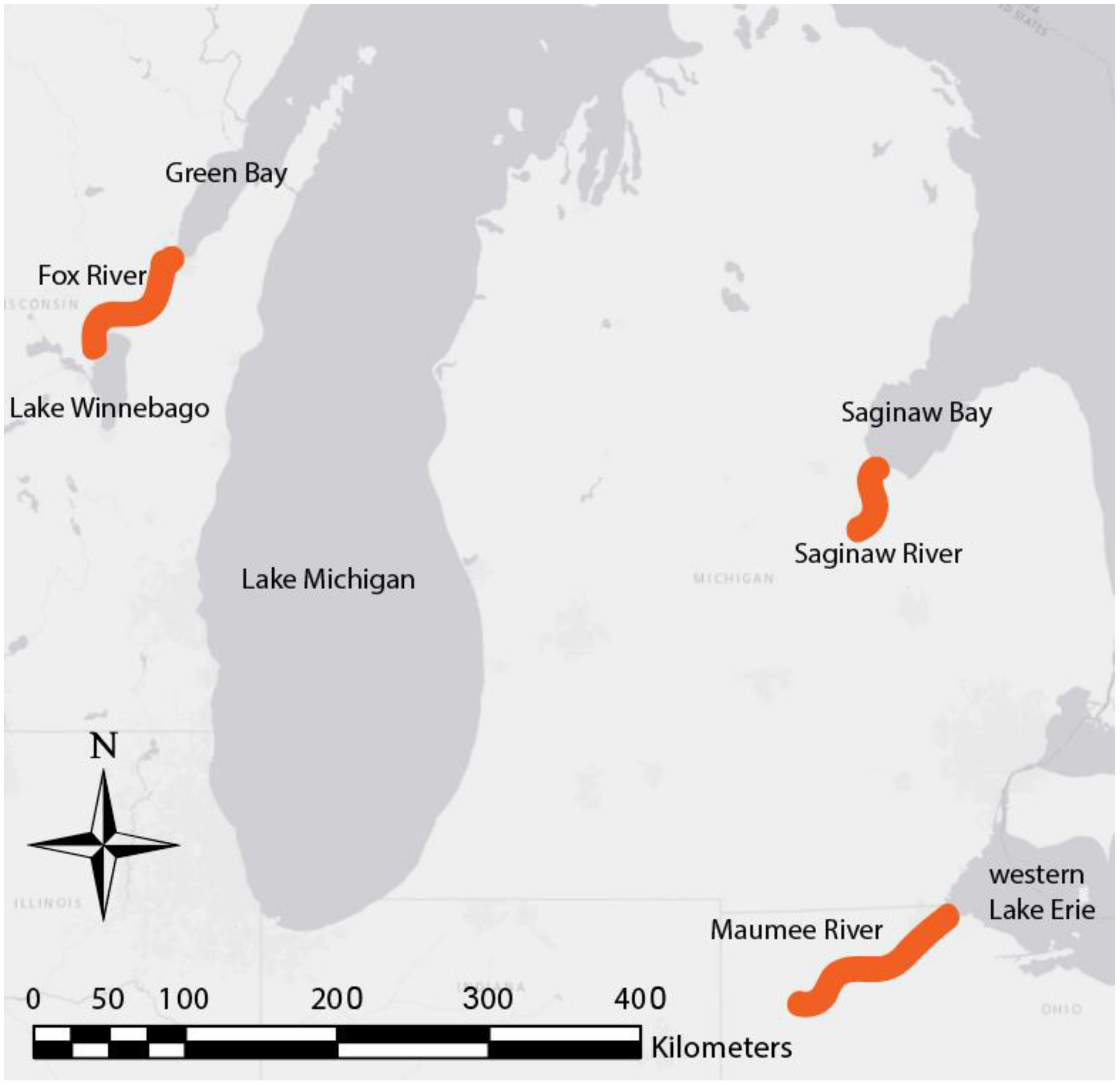
2.1. Study Site

The Laurentian Great Lakes, located in central North America, are a series of interconnected lakes that connect to the Atlantic Ocean through the Saint Lawrence River. Together the five Great Lakes contain 21% of the Earth’s freshwater by volume. There are three sub-basins of the Great Lakes that routinely have cyanobacteria blooms: western Lake Erie, Saginaw Bay, and Green Bay [5]. The three sub-basins each have one river that delivers the preponderance of nutrients: the Maumee River into western Lake Erie, the Saginaw River into Saginaw Bay, and the Fox River into Green Bay. This paper primarily looked at the cyanobacteria bloom phenology of Green Bay, which is a sub-basin of Lake Michigan (Figure 1). Saginaw Bay and western Lake Erie were considered for comparative purposes. Wynne and Stumpf [20,23] and Wynne et al. [19] previously examined the bloom phenologies in western Lake Erie and Saginaw Bay, respectively.

2.2. Satellite Imagery

Satellite imagery has long been shown useful for monitoring and describing the abundance of cyanobacteria blooms and is a key component of the data presented in this manuscript. The algorithm used in this study to estimate the cyanobacterial biomass is a derivation of the Cyanobacterial Index (CI), initially developed by Wynne et al. [24,25], for use with MERIS imagery. The CI is calculated following Equation (1).
CI = [ρs(681) − ρs(665) − (ρs(709) − ρs(665))((681 − 665)/(709 − 665)] (−1)
where CI, when positive, is the dimensionless Cyanobacterial Index, ρs is the Rayleigh corrected bi-directional reflectance, and the parenthetical is the MERIS wavelength expressed in nanometers. The CI is a metric of the chlorophyll-a (chla) absorption around 681 nm. Cyanobacteria have the majority of their chla in non-fluorescing photosystem I, whereas most phytoplankton have the majority of their chla in fluorescing photosystem II [27]. The algorithm is constructed so that if chla is estimated to be present but fluorescence is low (or absent), it indicates a predominance of cyanobacteria. In this case, the algorithm returns a positive CI value. When chla fluorescence is present, Equation (1) is negative, and the value is assumed to represent a bloom not dominated by cyanobacteria. There are, however, some cases where fluorescence is low and chla estimates are high even though no cyanobacteria are present. This typical occurs when very small sized eukaryotic phytoplankton, such as chlorophytes, comprise a significant component of the phytoplankton assemblage and/or when mixed blooms (e.g., diatoms, green algae, cyanobacteria, and others) are present and is associated with increased light scattering that can lead to false positives in the CI algorithm [25]. This may be a major challenge for Green Bay as it commonly experiences mixed blooms [6]. In contrast, western Lake Erie blooms are consistently dominated by cyanobacteria, primarily of the species Microcystis [6,28] indicating there may be differences in model outputs for these two systems.
This issue of false positive cyanobacterial estimates was addressed by including an additional spectral condition. Lunetta et al. [29] separated the CI into two component parts; The CI due to the cyanobacteria population (CIcyano) and the CI due to the biomass that is not comprised of cyanobacteria (CInoncyano) using spectral evidence of phycocyanin. This separation was based on the second derivative around the 665 nm band according to Equation (2).
S 2 d 665 = ρ s 665 ρ s 620 ρ s 681 ρ s 620 665 620 681 620
If the quantity of S2d(665) is positive, phycocyanin, an indicator for cyanobacteria was present. The rationale behind using S2d(665) is based on the 620 nm band being near the absorption peak of phycocyanin, which is a key photosynthetic pigment unique to cyanobacteria [30]. Without phycocyanin, the S2d(665) is negative, indicating a population of low fluorescing non-cyanobacteria plankton. The presence of phycocyanin will depress ρs(620), causing S2d(665) to be positive, which would indicate cyanobacteria. Consequently, if the S2d(665) is negative, phycocyanin is assumed to be absent and the CI value is set to be zero. Mathews and Odermatt [31] used an equivalent algorithm for determining cyanobacteria biomass. It should be noted that the separation using S2d(665) is not possible using ocean color sensors that lack the band at 620 nm (such as the Moderate Resolution Imaging Spectroradiometer [MODIS]). This limits the analysis of mixed populations to the MERIS satellite data, and its replacement, the Ocean Land Color Imager (OLCI).
MERIS satellite data was processed in methods detailed in Wynne et al. [32]. Clouds were masked and 10-day composites were made for each year during the bloom period using the maximum value of the CIcyano at each pixel. The CIcyano algorithm was then used to create 15 separate 10-day composites from the bloom season [21,23], which is defined here as the time period between June 1 and October 31. Each month contains three 10-day composites, with the final composite of a 31-day month being an 11-day composite (Table 1). When a metric of annual bloom intensity was needed the maximum integrated value of that year’s 10-day composite was used to represent the annual CIcyano. The integrated CIcyano was calculated by summing up all of the pixel values with a CIcyano > 0 [33]. There are several advantages to utilizing maximum value 10-day composites. The first advantage is that the composite reduces cloud interference, and therefore, reduces the data to a systematic set of generally cloud-free images [21]. The second key advantage is that the composites facilitate estimation of areal biomass. When winds are strong (>7.7 m s−1, or stress of 0.1 Pa), the bloom is mixed through the water column, diluting the surface concentration [25,34]. Under calm winds, however, Microcystis floats upward forming dense accumulations visible on the surface of the lake [35]. It should be noted that other genera of cyanobacteria can regulate their cell density, which effects their vertical distribution in the water column, as noted by Brookes et al. [36] for Anabaena circinalis. The surface concentration of the CIcyano estimated from satellite during calm conditions therefore represents the cyanobacteria that is present in the water column [26], whereas the concentration detected during high winds underestimates the water column biomass. Typically, during any 10-day period in the summer, there is a period of calm and clear weather [37], which allows an estimate of total cyanobacteria biomass. The cells return to the surface within 24–48 h following a wind event. The bands used for the algorithm quantify concentration within one meter of the surface in the clearest water [38], and less as turbidity increases (usually because of the bloom), therefore any material less than the optical depth will not be visible by satellite. Finally, using a 10-day composite makes biological sense, as the doubling time for Microcystis (the dominant genus of cyanobacteria in the Great Lakes) can be as low as 10 days in the Great Lakes region [39]. Wilson et al. [40] reported growth rates of 0.13 to 0.46 day−1.
Because chlorophyll-a absorbs more strongly than phycocyanin, Equation (1) algorithm has a larger dynamic range compared to Equation (2) and is a more sensitive metric for detecting cyanobacteria, particularly when cyanobacteria dominate the assemblage with little contribution by other phytoplankton groups [32].

2.3. Environmental Data

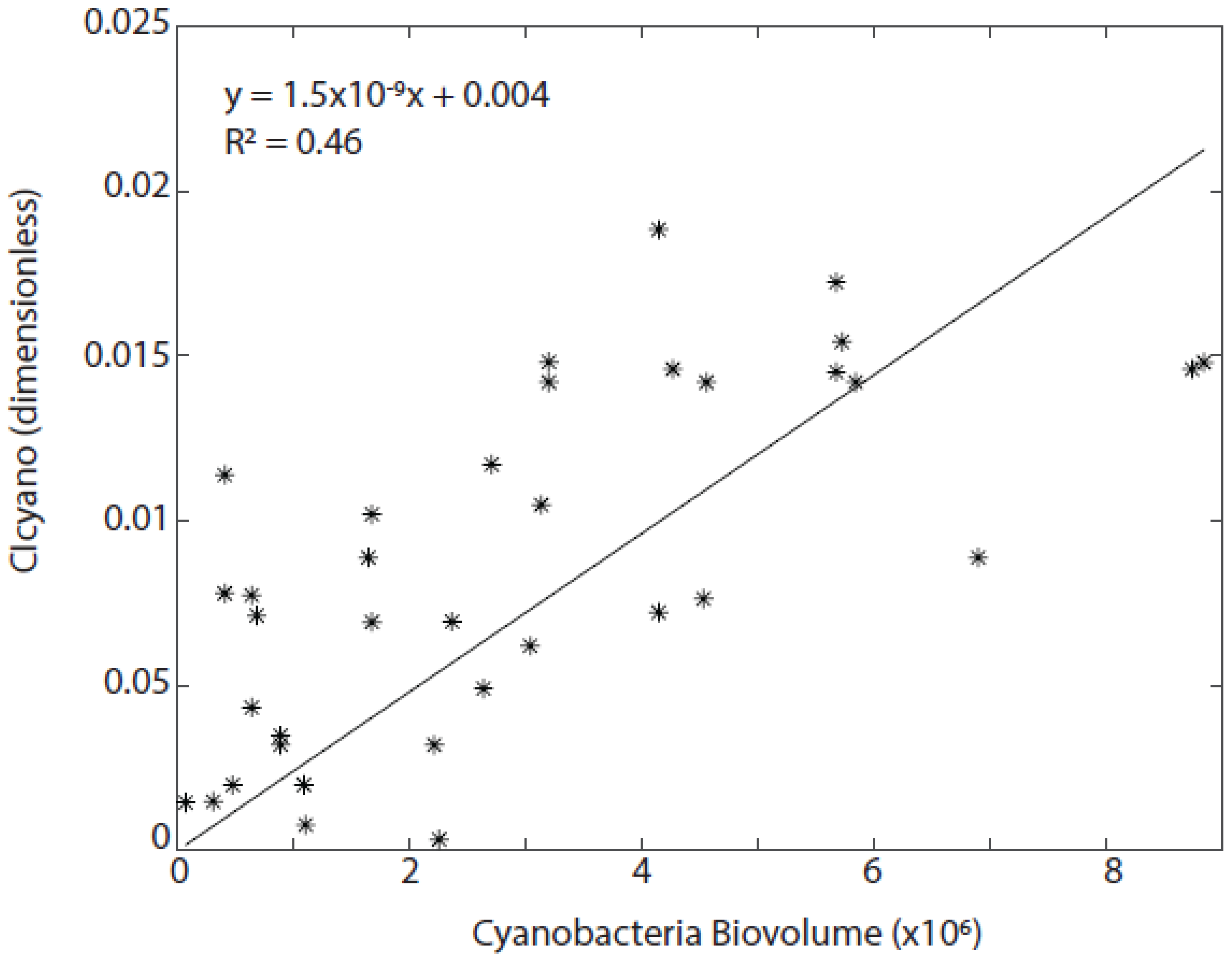
2.3.1. Biovolume Enumeration

The performance of the CIcyano algorithm (Equation (2)) for estimating cyanobacterial blooms in Green Bay was validated using field samples collected during the summers of 2004, 2005, 2006, 2007, 2010, and 2011 at five locations. These locations have been determined during previous studies to adequately sample the trophic gradient from the mouth of the Fox River to just south of Sturgeon Bay, where the waters from Green Bay mix with those of Lake Michigan proper (Figure 1; [41]). Surface phytoplankton samples were collected approximately biweekly each year from June through August. Duplicate integrated samples were collected from the top 4 m of the water column using a submersible pump (or to just above the bottom at sites shallower than 4 m). Samples were transported in opaque bottles kept on ice in the dark until returned to the laboratory later the same day, and then preserved in 1% Lugol’s solution. In the laboratory replicate subsamples (15–50 mL, depending on sample concentration) for phytoplankton identification and enumeration were examined using settling chambers viewed on an inverted microscope or on permanent slides made by filtering subsamples onto membrane filters (0.45 µm pore size) under low vacuum. Filters were cleared with immersion oil, sealed with Permount and enumerated at 100–500 × magnification. Cell linear dimensions were determined with an ocular micrometer and used to estimate cell biovolume based on published relationships between linear dimensions and volume [42]. Biovolume data were obtained for three classes of algae: diatoms, green algae, and cyanobacteria, as well as an “other” category. These data where then used to validate the CIcyano algorithm for Green Bay.

2.3.2. Quantifying Cyanobacterial from Other Planktonic Groups and Algorithmic Validation

The field collected samples were matched with the closest clear overflight image. The difference in the time the field sample and satellite sample were collected was plus or minus one day. It should be noted that the locations of surface blooms are highly dynamic depending on wind and current speed even at the scale of minutes to hours. For example, Kutser [43] took two samples on either side of a research vessel and the cyanobacteria enumeration varied by an order of magnitude. This patchiness can become even more pronounced in imagery as there is approximately 12 orders of magnitude in a satellite pixel (1100 m by 1100 m by 0.5 m) relative to a 5 mL water sample used for field enumeration. Another issue is that the satellite may be mis-navigated. The actual geolocation of a pixel may be off and the water sample may not be from the exact spot sampled by the satellite. Finally, the error of the field sampling techniques must be kept in mind. For these data the error in the biovolume was given to be approximately 30% [44]. All these factors can introduce variation in the perceived relationship between algorithm results and the field-collected biovolume data.
Next, a 3 × 3 satellite pixel box around the biovolume sample point was extracted. The median of this 3 × 3 pixel wide box (3300 m × 3300 m) was then calculated as long as there was at least one suitable pixel available. Any pixels that were suspected of land contamination, sun glint, or cloud/cloud shadow were removed from further analysis. Overall, there were 69 different samples that met these criteria. The percentage of each of the four functional groups (Cyanobacteria, Greens, Diatoms, and others) were calculated.

2.4. Climatology

The Green Bay CIcyano climatology was created from the 10-day composites listed in Table 1. All data was extracted from Green Bay, and all pixels that had a positive CImax value were summed, to yield an integrated CIcyano value. The CImax was calculated as the maximum integrated 10-day composite from each year. The CImax for each region (Green Bay, Saginaw Bay, and western Lake Erie) were calculated in the same fashion over the 10 years of the MERIS timeseries. The mean, median, mode and standard deviation of the bloom initiation date were also calculated for Green Bay, as well as for Saginaw Bay and western Lake Erie. The bloom initiation date was defined as when the integrated CIcyano from a 10-day composite was above a value of one. In the event that the CIcyano did not achieve a value of one in any given year the CImax was used in its place. The interannual variability was estimated for Green Bay, western Lake Erie and Saginaw Bay by dividing the highest CImax by the lowest CImax for each basin.

2.5. Model Building in Green Bay

Building empirical models using available and routinely monitored environmental data that can predict cyanobacterial blooms in the Laurentian Great Lakes can have a number of positive benefits. These include the reduction in the detrimental economic and environmental impacts of the blooms and a better understanding of bloom dynamics which will help guide future mitigation efforts to reduce bloom intensities. Toward this end the previously described satellite derived cyanobacterial bloom (CIcyano) time series was used in conjunction with river discharge data from the United States Geological Survey (USGS) and corresponding modeled environmental datasets from NASA’s Giovanni database (Giovanni is an acronym for the GES-DISC [Goddard Earth Sciences Data and Information Services Center] Interactive Online Visualization ANd aNalysis Infrastructure) to identify the most informative environmental factors upon which bloom models could be based [45].

2.6. River Discharge

The first environmental factor extracted for analysis was river discharge (river_Q), which has been shown to be a good estimate of P-loading, one of the primary nutrients limiting phytoplankton growth in these systems [46,47]. Because Green Bay has the majority of P-loading from the Fox River it is reasonable to hypothesize a strong correlation between the discharge of the Fox River and cyanobacterial biomass in Green Bay. The river discharge for the Fox River was obtained from the USGS station 04,084,445 at Appleton, Wisconsin. The monthly option for the discharge statistics was selected and mean monthly flow rates were calculated. The four monthly combinations that were investigated were (1) water year (1 October–30 September); (2) March–June; (3) March–May; and (4) March–July. These combinations of months were used to test for correlation between annual CIcyano concentrations and mean monthly flow rates.

2.7. Other Environmental Data from NASA Giovanni

Various additional modeled environmental factors were considered. These parameters were from the NASA Giovanni database. Many parameters were considered but the four that were selected for further analysis were Gelbstoff and detrital absorption (adg), meridional wind speed (vgrd), latent heat flux (lhtflsfc), and night-time sea surface temperature (nsst). Each parameter was downloaded as an area averaged monthly product for Green Bay (−87.9375, 44.5625, −87.6042, 44.9375), western Lake Erie (−83.55, 41.45, −82.55, 42.05), and Saginaw Bay (−84.0625, 43.5625, −83.2292, 44.3125). The gelbstoff +and detrital absorption product was downloaded as 8-day composites from Giovanni, as the monthly mean product was unavailable, and the monthly mean was estimated from the available 8-day composites instead. The Giovanni data corresponding to the bloom year (defined here as June–October) were considered. The raw data downloaded from Giovanni for each region can be found in the Supplementary Materials. The NASA Giovanni variables are described in Section 2.7. The monthly Giovanni data were correlated with the monthly CIcyano data product. The annual data were used in a Principal Components Analysis (PCA) in an effort to determine the factors that may lead to bloom formation.

2.7.1. Water Temperature

Water temperature (nsst) was selected as it is a well-documented driver of cyanobacteria blooms [48,49]. Wynne et al. [25] showed that blooms of Microcystis in western Lake Erie ended once water temperature dipped below 15 °C, and it would be logical that the Microcystis blooms in Green Bay would follow similar trends.

2.7.2. Wind Speed

Wind speed can be used as a proxy for vertical mixing and turbulence. Vertical mixing and turbulence have been shown to have negative impacts on cyanobacteria bloom abundance and that blooms are more prevalent under low turbulence [48,49,50]. The meridional wind speed (vgrd) was used as a proxy for wind mixing/turbulence. The meridional wind (v-direction) more closely follows the axis of Green Bay relative to the zonal wind speed (u-direction; Figure 1). However, increased turbulence and wind stress is not necessarily detrimental to the formation of cyanobacteria blooms. In fact, it has been suggested that an increase in turbulence may actually promote cyanobacteria blooms [51], as under turbulent conditions cyanobacteria may form larger colonies which can counteract some of the turbulence effects on buoyancy. Furthermore, it has been suggested that under high turbulence cyanobacteria can produce an increase in toxin production which can negatively affect other algae thereby giving cyanobacteria a competitive advantage [52].

2.7.3. Gelbstoff and Detrital Absorption

Gelbstoff is also called Colored Dissolved Organic Material (CDOM; [53]). The absorption of gelbstoff and non-algal particles (detrital absorption) is commonly measured in the blue wavelengths and can be used to partially describe the apparent optical properties of a body of water [54,55]. Kirk [53] found that gelbstoff absorption was the dominating optical influence in inland waters, with gelbstoff absorbing 60–80% of photosynthetically active radiation. Here, we employed the gelbstoff and detrital absorption at 443 nm (adg) as a measure of light attenuation. Calculated phytoplankton absorbance was 2–3 times smaller than gelbstoff absorption during the whole time series in Green Bay, therefore gelbstoff absorption was found to be a more suitable parameter to evaluate. Gelbstoff absorbs blue light strongly and it is hypothesized that an increase in Gelbstoff absorption will lead to a competitive advantage of cyanobacteria relative to diatoms, their primary competitor. This is because cyanobacteria have phycocyanin, which absorbs light in the red-orange wavelengths, while diatoms generally absorb light strongly between 400–500 nm (blue light) with carotenoids and chla [56]. Cyanobacteria can also regulate their buoyancy and can migrate up or down the water column under calm conditions to find optimal light conditions whereas diatoms are negatively buoyant and sink.

2.7.4. Latent Heat Flux

The latent heat flux (lftflsfc) is determined by the latent heat of vaporization, the stability turbulent exchange coefficient at 2 m above the surface, the saturation humidity, and the specific humidity of the air 2 m above the surface [57]. Latent heat flux has been shown to affect the phytoplankton community structure, by affecting the stratification of water [58,59,60,61], as cyanobacteria are affected by water stratification [62].

2.8. Statistical Comparisons between Basins

2.8.1. Differences in Green Bay Relative to Western Lake Erie and Saginaw Bay

In an effort to examine and quantify potential differences in these three catchments, a Principal Components Analysis (PCA) was performed using the ggbiplot package in R. The ggbiplot is a bi plot as it delivers information on loadings (which are shown as vectors or arrows) as well as scores (which are the points or years as is the case of the PCAs shown here). The origin represents the average across each variable and for each object across all variables. The length of the arrows in the plot are directly proportional to the variability of the two shown principal components. The angle between the vectors represents the correlation of those two vectors (e.g., if the angle is zero or 180 degrees the vectors are colinear, whereas if they are 90 degrees they are orthogonal and show lack of correlation) [63]. The ellipses that are shown in the PCA are the 68% confidence intervals of a point (i.e., any given year) falling into a certain class [64].
The input variables in the PCA are those listed in Section 2.7 along with the river discharge from the USGS gage stations at the Maumee (USGS station 04193500), Saginaw (USGS station 04157005), and Fox (USGS station 04084445) Rivers. The Maumee River is the main source of P to the western basin of Lake Erie [47], while the Saginaw River is the main source of P to Saginaw Bay [65]. Various means from the river discharge out of the Fox River were calculated, including: the mean from March–June, the mean from March–July, and the mean for the water year.

2.8.2. High Bloom Years vs. Low Bloom Years

Further PCAs were run to determine if high bloom years could be separated from low bloom years. The input data into the PCA was the river discharge and all the Giovanni parameters in Section 2.7. Two separate bloom scenarios were considered. In the first scenario two classes: high bloom and low bloom, were considered where the 5 years with the highest annual CIcyano values were considered as high bloom years, and the 5 years with the lowest CIcyano values were considered low bloom years. In the second scenario, a final PCA was considered to separate the extremely small CIcyano years of 2009 and 2010 from the remaining years in Green Bay. These were parsed out from the other years in attempt to determine what characteristics led to essentially no blooms in those two years. These analyses were run for Green Bay and then for comparison purposes they were run for western Lake Erie. Saginaw Bay was not considered as there was very little interannual variability in bloom sizes [5,20].

3. Results

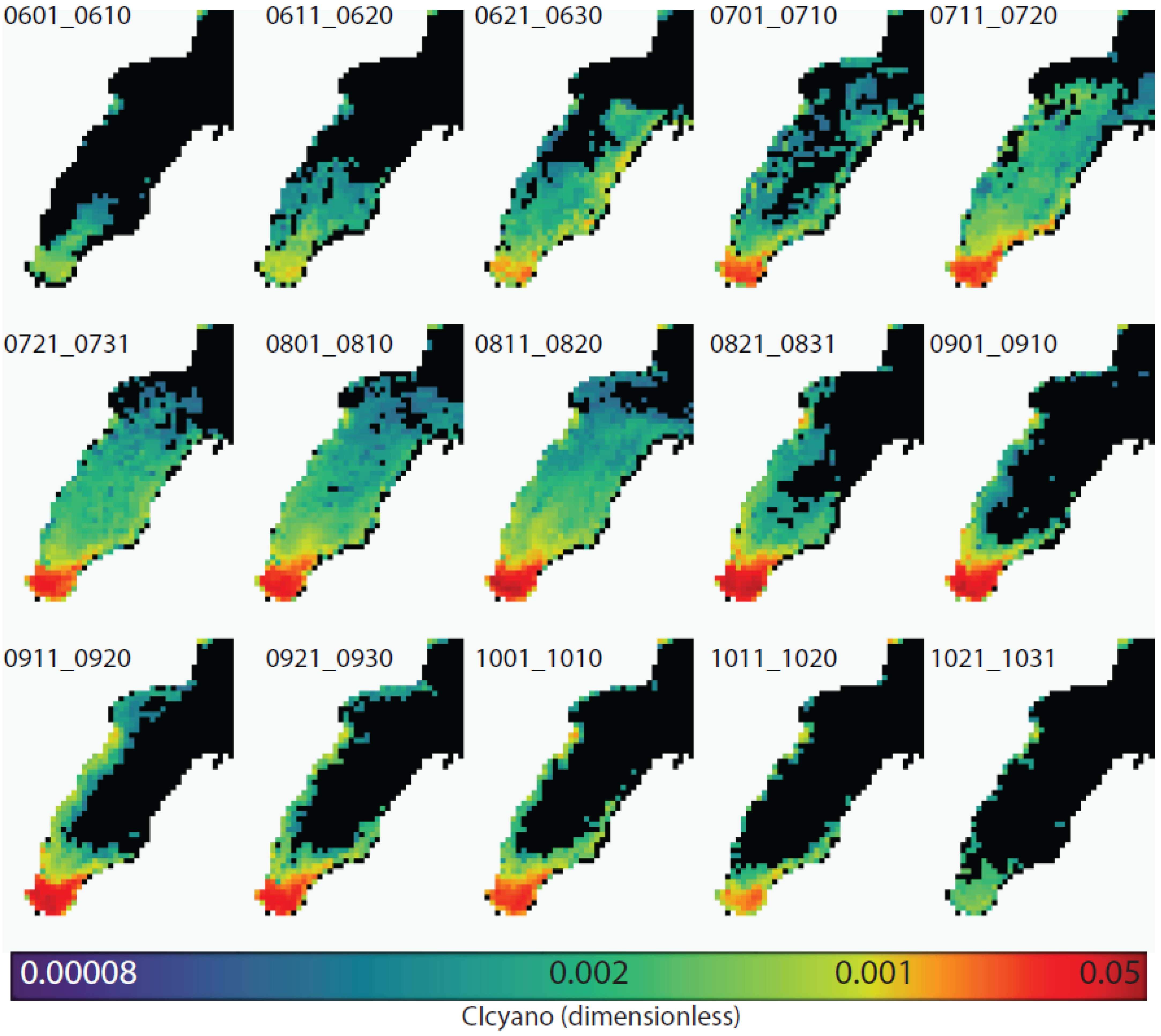
3.1. Estimating Cyanobacteria Using CIcyano

If a system is consistently dominated by cyanobacteria during the bloom season, using the CI rather than the CIcyano allows detection of a broader range of cyanobacterial biomass [20]. In Saginaw Bay, and particularly in western Lake Erie, false positives from eukaryotic phytoplankton were not an issue, and CI has been the preferred metric [20]. Figure 2 shows the relationship between the CI and the CIcyano (estimated using Equation (2)) for western Lake Erie, Saginaw Bay, and Green Bay derived from the 10-year MERIS timeseries of 10-day composites. Figure 2A shows that the relationship between CI and CIcyano from western Lake Erie had both the tightest fit (i.e., the highest R2) and a slope that was the closest to unity (i.e., 1), consistent with the assemblages being mostly dominated primarily by cyanobacteria. Figure 2B shows that the relationship from Saginaw Bay is weaker, indicating that the observed blooms more often represent a mixed assemblage with significant contributions by other non-cyanobacterial planktonic groups. Figure 2C shows the relationship in Green Bay which exhibited the weakest correlation, which necessitates the use of the CIcyano algorithm.

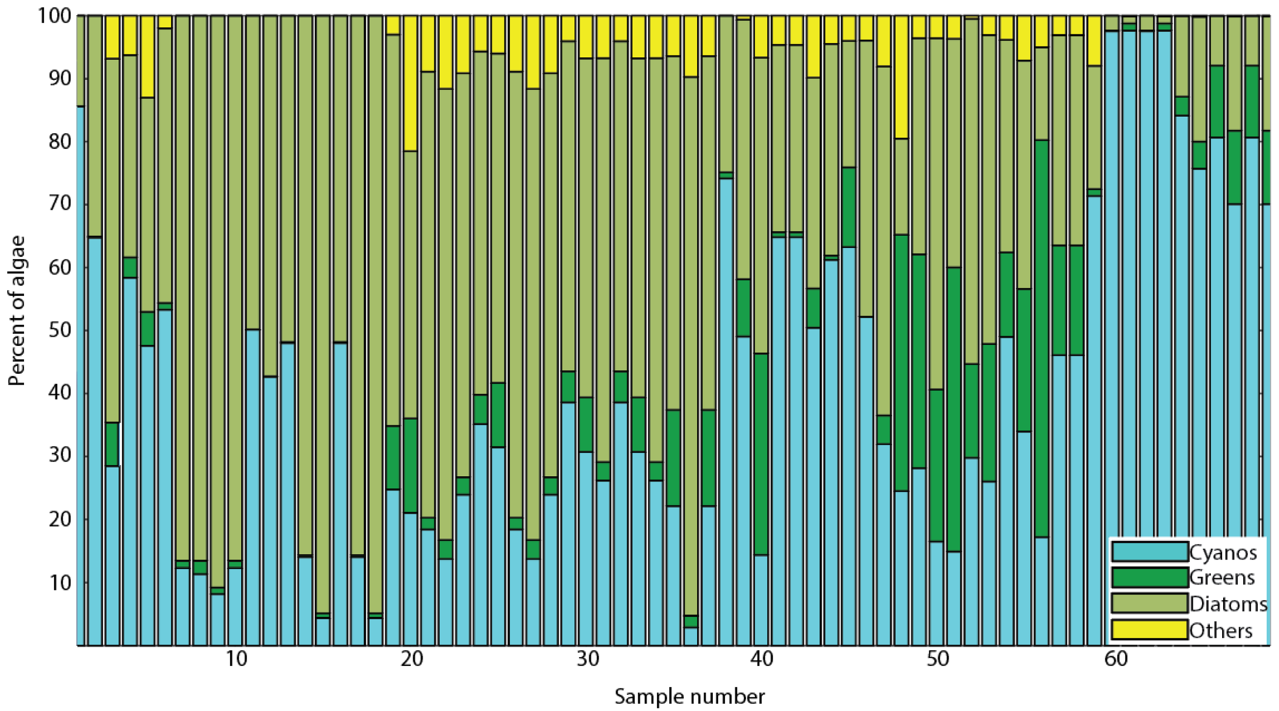
3.2. Algal Diversity in Green Bay

Summer blooms in Green Bay are not necessarily dominated by cyanobacteria like they are in western Lake Erie and Saginaw Bay [5]. There were 69 biovolume samples that had a corresponding remotely sensed image. Percent community composition by phytoplankton class was determined for each sample with corresponding imagery (Figure 3). Figure 3 shows that generally there is a competition between cyanobacteria and diatoms, with greens and other algae contributing a smaller percentage of the overall algal assemblage. Of the 69 samples with imagery, 36 had a positive CIcyano relationship. Least squares regression was done with the samples that had a positive CIcyano against the cyanobacteria biovolume (Figure 4), giving a resultant R2 = 0.46.
The CI versus CIcyano regressions suggest that there were mixed blooms of phytoplankton in Green Bay, whereas in Saginaw Bay and western Lake Erie where cyanobacteria blooms were generally more dominated by cyanobacteria (Figure 2, [5,20]). The biovolume data per phytoplankton class (Figure 3) further reinforces this observation. This suggests that there is something fundamentally different in the physical and/or biogeochemical environment in Green Bay relative to western Lake Erie and Saginaw Bay.

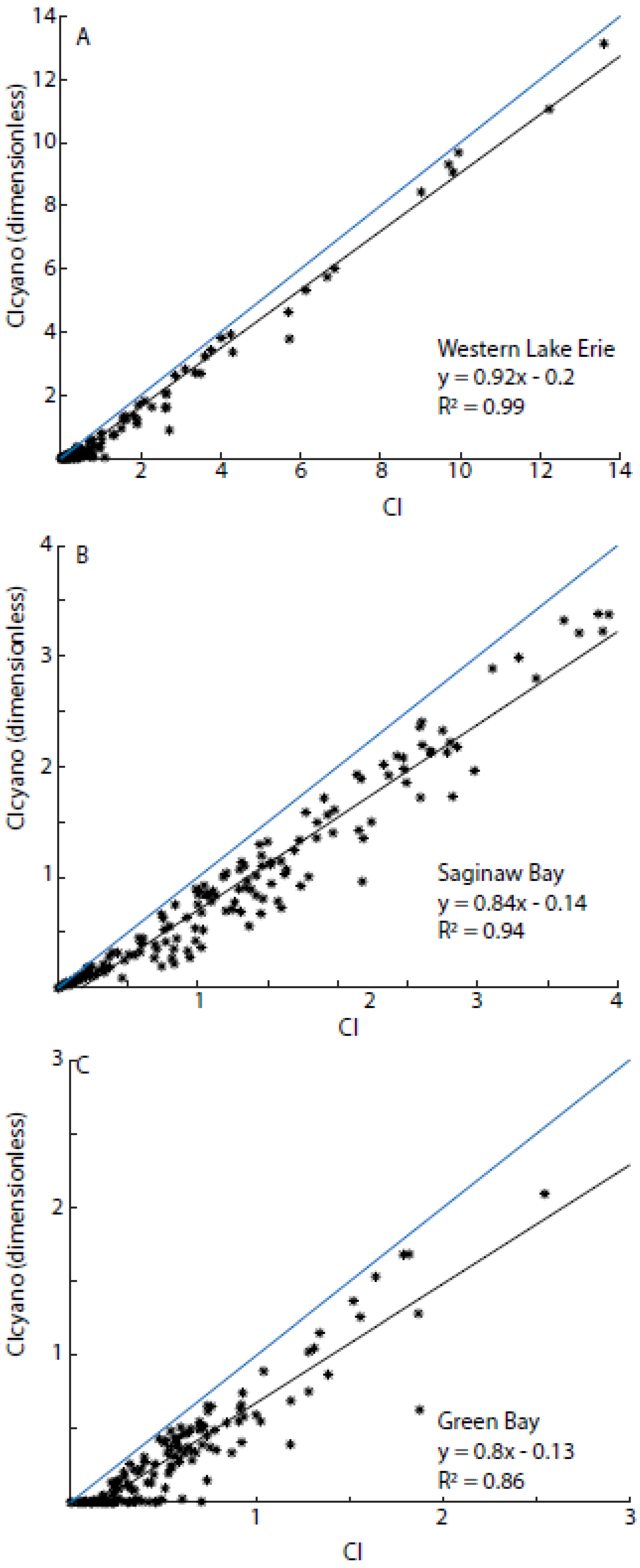
3.3. Algorithmic Validation

The CIcyano algorithm was validated from the satellite imagery described in Section 2.2 and the environmental data described in Section 2.3. Green Bay appears to have a predominately mixed planktonic community assemblage (Figure 3), which argues for the use of the CIcyano algorithm over the CI algorithm. To estimate the efficacy of the CIcyano algorithm the linear regression was performed between the biovolume (Section 2.3.1) and the CIcyano algorithm (Section 2.2).

3.4. Climatological Analysis

Green Bay blooms typically show an increase in area and extent through June and July (Figure 5 and Figure 6). Climatological means from 10-day composites with CIcyano were averaged across 10 years of input data from 2002–2011 in image format (Figure 5) and were extracted to create a time series (Figure 6). Generally, blooms peak in late July to early August in Green Bay. The blooms in Green Bay reach their maximum value, on average, during composite number 6.7 (~July 28) (Table 2). In 2009 and 2010, very little signal from the CIcyano algorithm was detected.
One further analysis focusing on the interannual variability between Green Bay, Saginaw Bay, and western Lake Erie was done to look at variability within each system. The results from this analysis are shown in Table 3:
Western Lake Erie exhibited the largest range of interannual variability of the three basins considered here (Table 3). Saginaw Bay experienced the lowest interannual variability using the methods described in Section 2.4. Figure 7 shows the timeseries of the annual CIcyano values from the three basins. The blooms in Green Bay tended to reach their peak on average 23 days before those in Saginaw Bay and 36 days before those in western Lake Erie using the methods described in Section 2.4.

3.5. Model Building

In an effort to build a predictive model, the first thing was to correlate the CImax with river discharge. The best river discharge model was March–June, which corresponded to results by Stumpf et al. [20]. However, the correlation between the CImax in Green Bay and the Fox River discharge (R2 = 0.14) was approximately five times lower than in western Lake Erie (Maumee River; R2 = 0.75 [20]) and was roughly equivalent to the relationship in Saginaw Bay (Saginaw River; R2 = 0.2 [19]).
With the river discharge model not having sufficient power to predict cyanobacteria blooms in Green Bay, the monthly averaged area NASA Giovanni data products were directly associated with the average monthly CIcyano product. To clarify the data source for each parameter used in model building is as follows: the CIcyano originated from the MERIS satellite imagery being used as an input into Equation (2), the river discharge data was directly measured by USGS discharge stations near each of the respective river mouths and downloaded directly from the USGS (see Section 2.6), and the NASA Giovanni output data (gelbstoff-absorption, Nighttime Sea-Surface Temperature, meridional windspeed, and latent heat flux) were downloaded directly from the NASA Giovanni project page and the downloaded data are available in the Supplemental Materials (see Section 2.7). The best relationship was with the gelbstoff absorption (adg), where R2 = 0.6. Unfortunately, this parameter is no easier to predict than the cyanobacteria blooms making the development of a predictive model challenging. The maximum CIcyano (i.e., the highest 10-day composite for each year) never occurred in June or October during the 10-year timeseries considered. Rerunning the correlations with those two months taken out of the Giovanni dataset, so the only remaining months were July, August, and September, yielded no better results with the average monthly CIcyano relative to the entire bloom season (June–October). Unlike in western Lake Erie, there was no reliable model between any variable and the annual CIcyano.

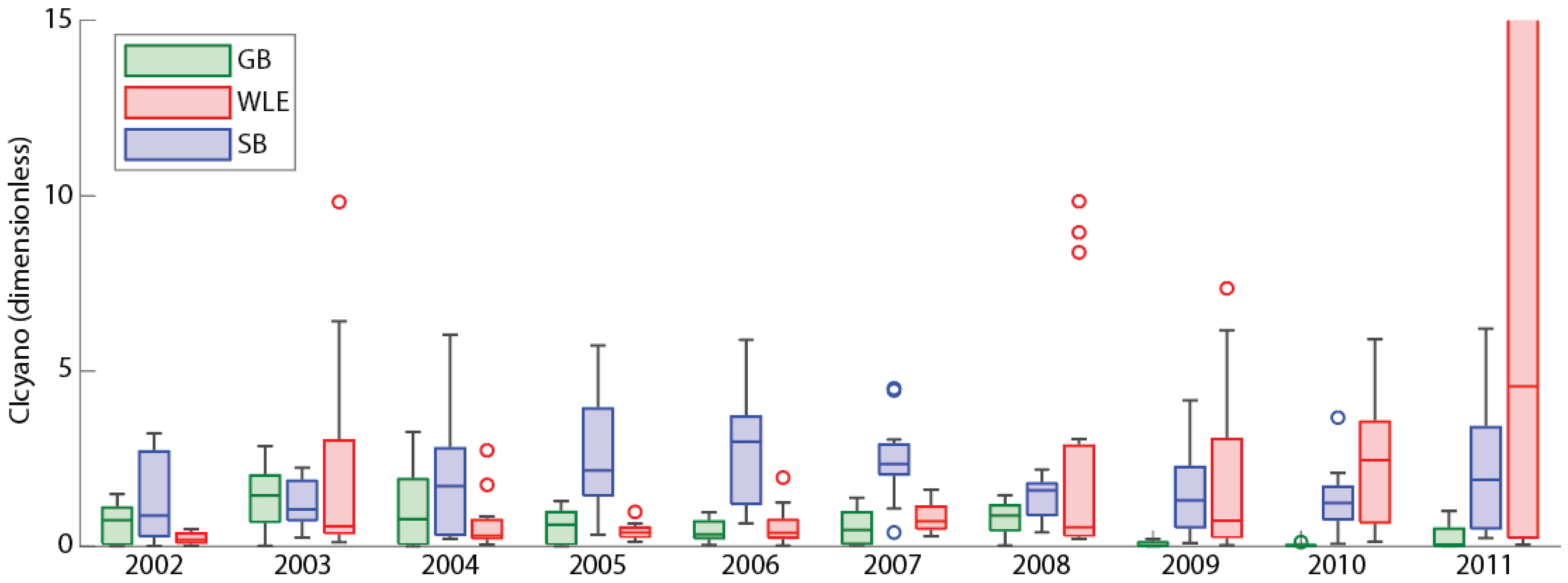
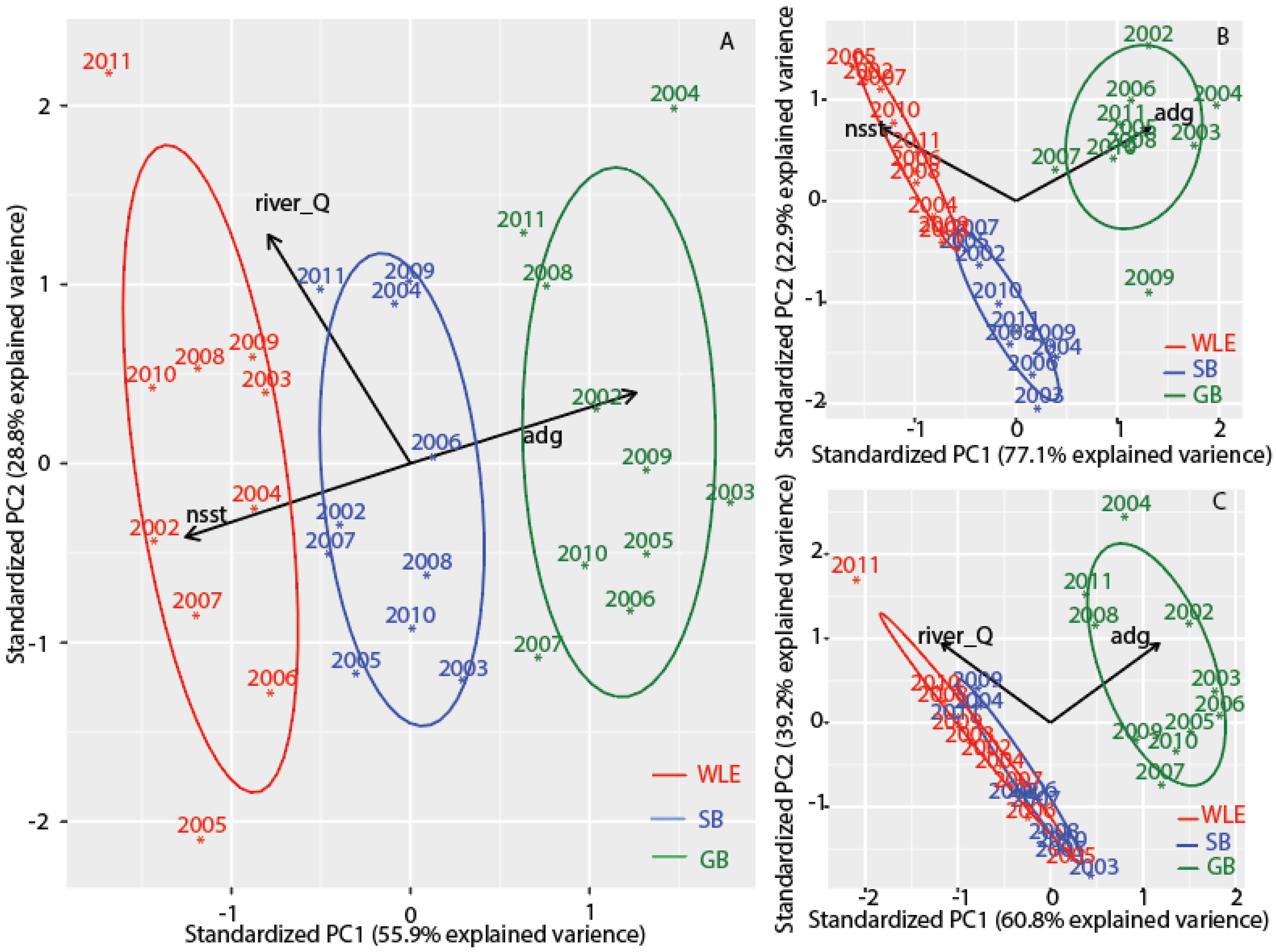
3.6. Comparisons with Western Lake Erie and Saginaw Bay

To compare the three different basins, a PCA was run. The purpose here is to see if it is possible to use previously discussed environmental parameters (Section 2.6 and Section 2.7) to separate the three basins from each other. The seasonal (June–October) averages were calculated using all the Giovanni parameters listed in Section 2.7 and were entered into a Principal Components Analysis (PCA), with a goal of separating Saginaw Bay, western Lake Erie, and Green Bay based on these data. The PCA can be used as a data elimination technique, and was run with three variables: the nsst, river_Q, and adg. This provided the best separation among the three water bodies (Figure 8A) without the risk of overfitting the data. The PCA was rerun using just the adg and the nsst (Figure 8B) and still had good separation of the water bodies. This indicates that Green Bay is colder and more turbid relative to western Lake Erie and Saginaw Bay. Saginaw Bay and western Lake Erie have similar Gelbstoff absorption, and water temperatures with western Lake Erie being slightly warmer than Saginaw Bay. The PCA was rerun a third time using River_Q and adg and showed excellent separation between Green Bay and the two other water bodies, but no real separation between western Lake Erie and Saginaw Bay (Figure 8C). This indicates that the river discharge shows very little contribution to Green Bay relative to Saginaw Bay and western Lake Erie, and that adg is perhaps the defining characteristic of Green Bay water based on the parameters examined.

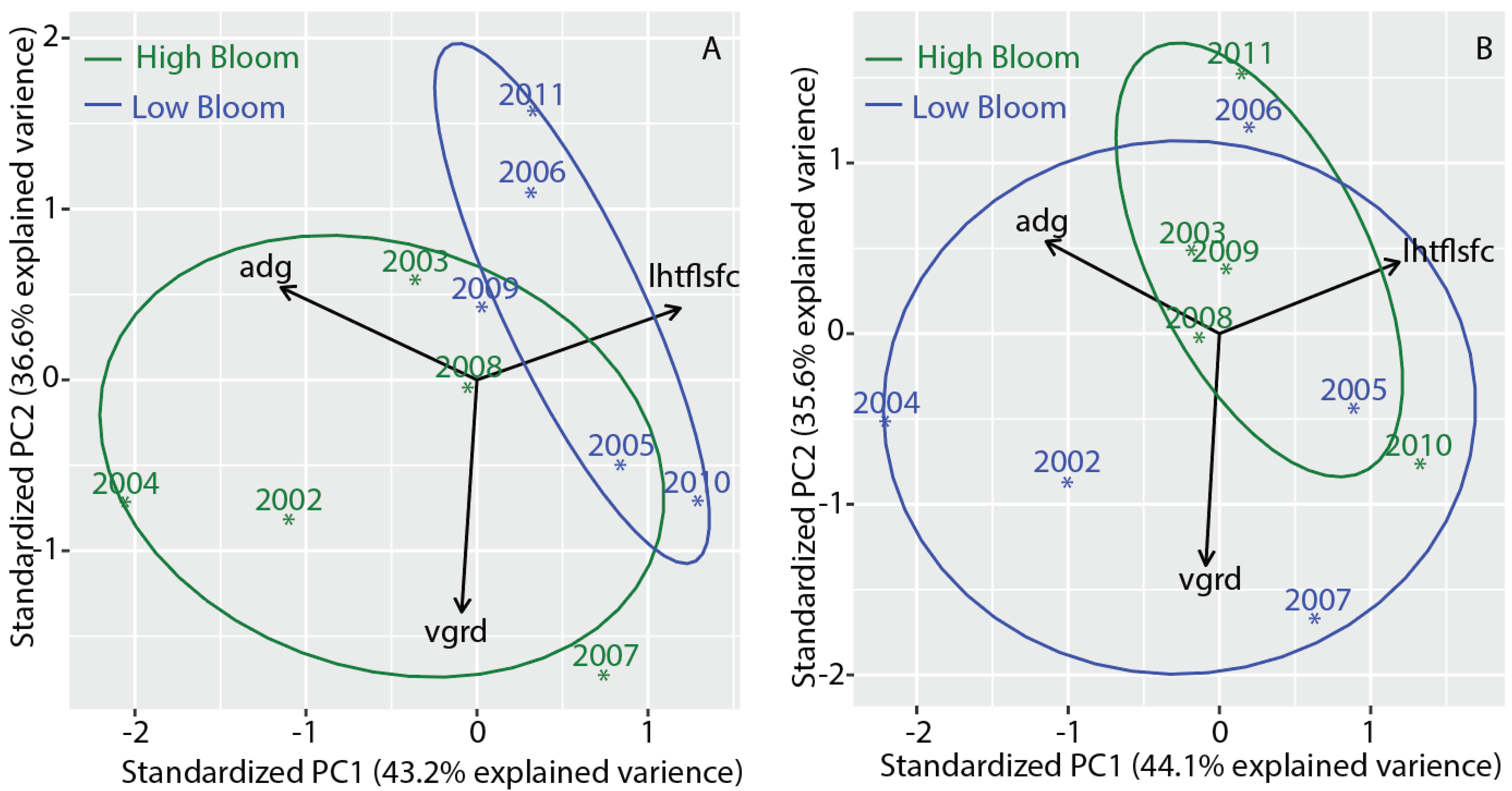
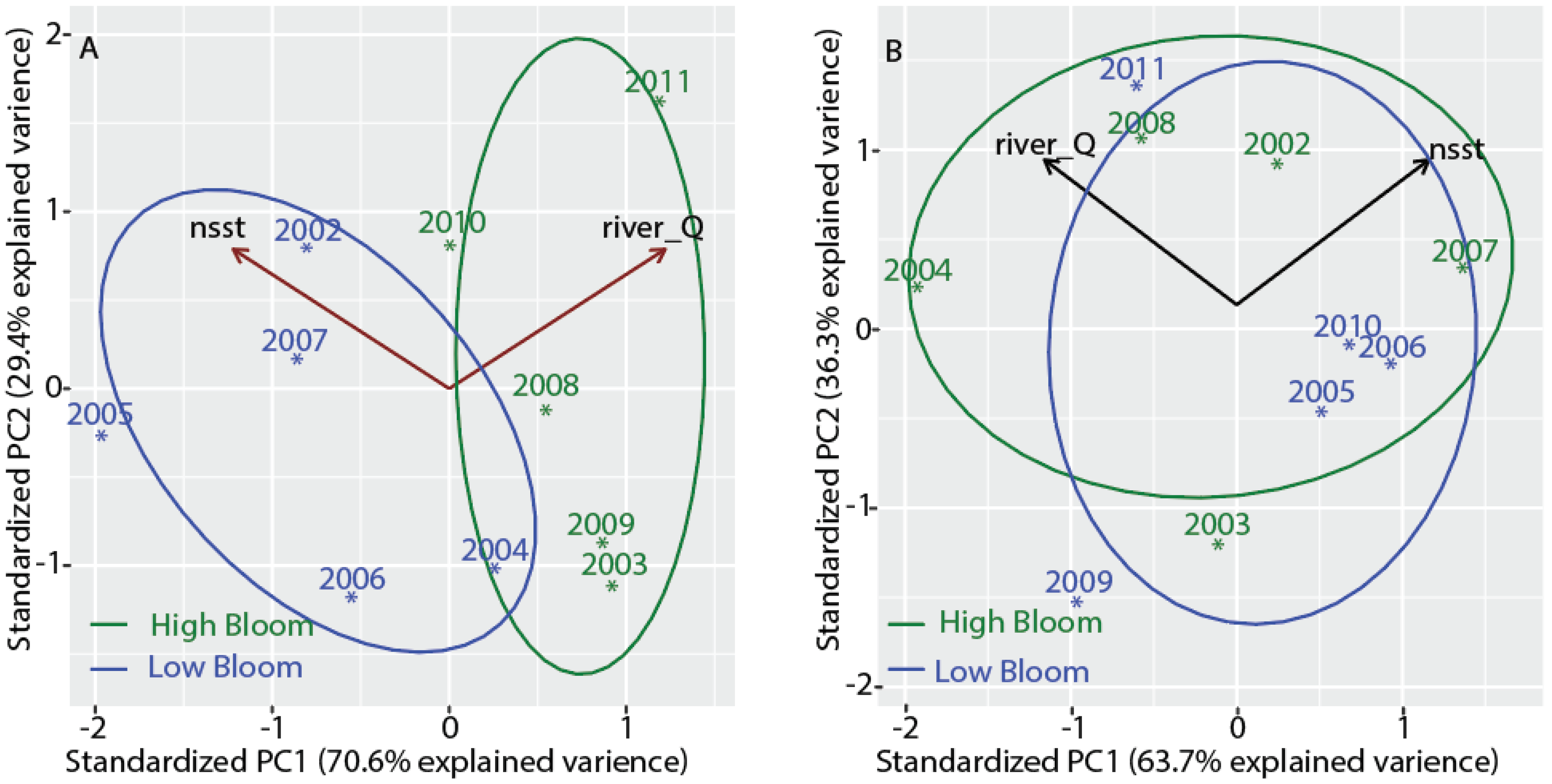
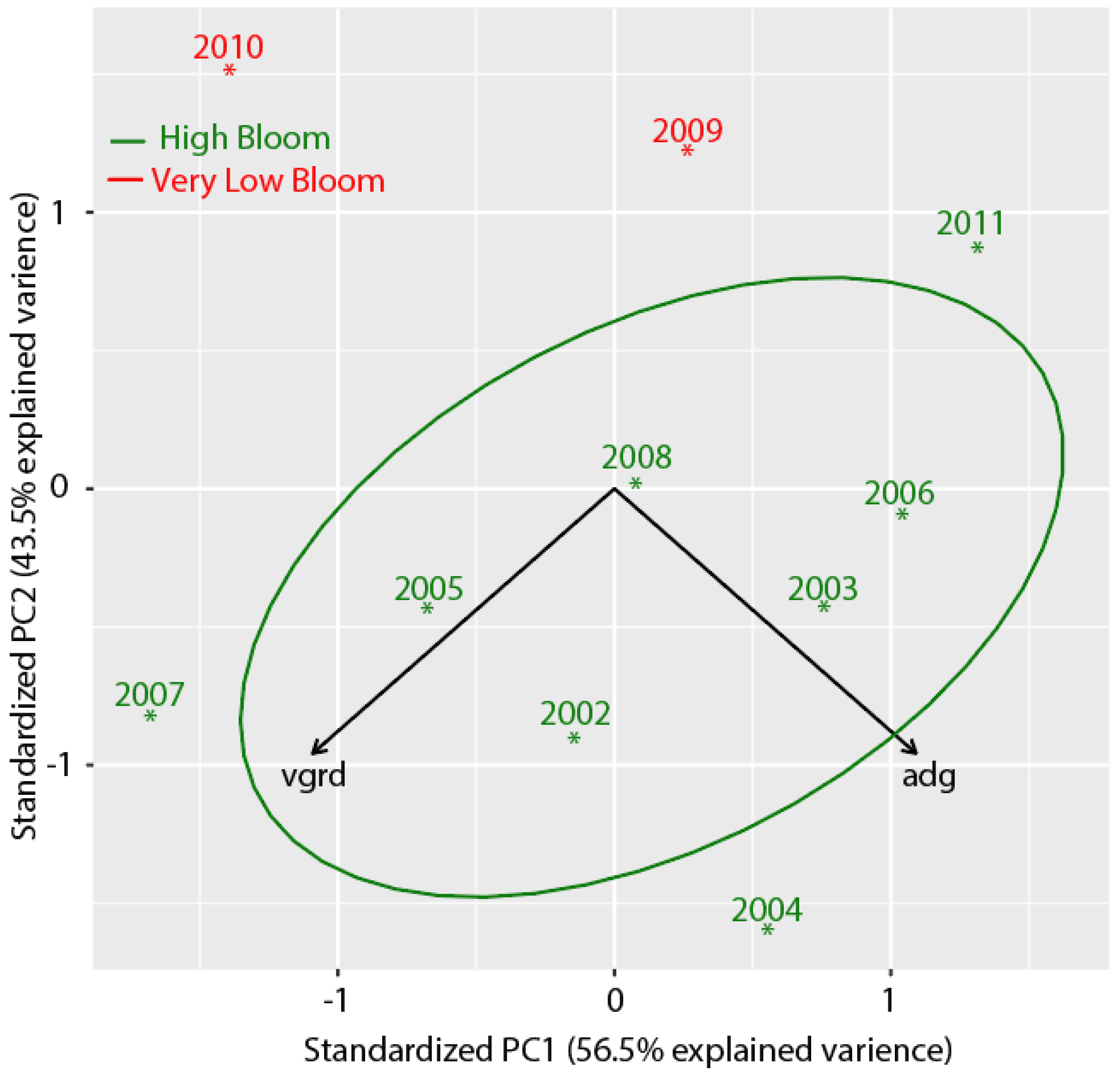
3.7. Separating High Bloom Years from Low Bloom Years

An additional set of PCAs were run to illustrate the differences between the high bloom years and low bloom years in Green Bay and then the analysis was repeated for comparison sake for western Lake Erie. The data were reduced as much as possible for this analysis, while still giving some measure of separation between the high bloom years and the low bloom years. Two separate PCAs were developed using the Giovanni parameters in Section 2.7, along with river discharge. The goal of the first PCA was to show the best separation for high bloom and low bloom years for Green Bay. The goal of the second PCA was to separate high bloom years and low bloom years for western Lake Erie. The PCA that effectively separated high and low bloom years in Green Bay was then run in western Lake Erie for comparison purposes, and likewise the PCA that separated high and low blooms in western Lake Erie was also run in Green Bay. Figure 9A shows the best separation between the high bloom and low bloom classes for Green Bay, and shows reasonable separation between the two classes. The same model shows poor separation between the high bloom and low bloom years in western Lake Erie (Figure 9B). The model uses lhtflsfc, adg, and vgrd. The vgrd is the meridional wind speed and aligns much better with the central axis of Green Bay than does western Lake Erie (Figure 1). The adg term has already been discussed in Section 2.7.3. The latent heat flux, a surrogate for stratification, shows importance in Green Bay. This may be as a result of Green Bay being both bathymetrically and optically deeper relative to western Lake Erie. Western Lake Erie has very little stratification [66] leading to the conclusion that latent heat flux is negligible in the formation of cyanobacteria blooms in western Lake Erie.
The best western Lake Erie model to separate high bloom years from low bloom years uses just two parameters: river discharge and nsst (Figure 10A). The same parameters used to separate the high bloom years from the low bloom years in western Lake Erie (Figure 10A) showed essentially no separation in Green Bay (Figure 10B). Of the five parameters selected for all of the PCAs run in this study (river_Q, nsst, vgrd, adg, and lhtflsfc), the two models in Figure 8 and Figure 10 showed no commonality, meaning that the blooms in Green Bay are governed by different parameters than the blooms in western Lake Erie.
A final PCA was used in an attempt to understand why there were very low blooms in Green Bay in 2009 and 2010. In this PCA high bloom class years were 2002–2008 and 2011, and very low bloom class years were 2009 and 2010. These two classes separated reasonably well with vgrd and adg. This implies that low meridional wind and low gelbstoff absorption led to years without blooms.

4. Discussion

In Green Bay, while cyanobacteria are relatively small in biomass, they show a high degree of interannual variability. However, there was considerable difficulty determining a useable model to predict annual cyanobacteria biomass from the suite of environmental parameters considered here. The three main issues preventing such a statistical model were: (1) a lack of annual data as the MERIS sensor only provided a 10-year dataset, (2) relatively small cyanobacterial biomasses, and (3) that cyanobacteria can co-occur with other phytoplankton.
From this study, it was clear that Green Bay has lower cyanobacteria concentrations relative to Saginaw Bay, which in turn has lower cyanobacteria concentrations relative to western Lake Erie. In spite of the very high variability of cyanobacteria blooms shown in Table 4, it has been noted that there is little interannual variability in respiration and gross primary productivity in Green Bay [67]. The average gross primary production of Green Bay is 288 mmol O2 m−2 day−1 [67] This is a factor of five higher than the gross primary production in Saginaw Bay of 40.6–65.1 mmol O2 m−2 day−1 reported by Fahnenstiel et al. [68]. While Saginaw Bay has higher cyanobacteria biomass relative to Green Bay, the primary production is higher in Green Bay further indicating the confounding issues of mixed phytoplankton assemblages present in Green Bay. Much of this variability in the cyanobacteria bloom is a result of having essentially little to no blooms in 2009 and 2010. Despite a lower standing stock of chlorophyll, it is still possible that the primary production exhibits similar rates in 2009 and 2010 than it is for the remaining years as the production was most likely based on increased concentrations of diatoms and green algae which are grazed more heavily than cyanobacteria [69]. The PCA shown in Figure 11 indicates that clearer waters with more wind stress invoked an ecological switch giving a competitive advantage to other functional types of phytoplankton (diatoms) over cyanobacteria.
The cyanobacterial biomass is much lower in Green Bay relative to Saginaw Bay and western Lake Erie, despite all three basins being similarly sized (Figure 1 and Figure 7). Cyanobacteria often co-occur with other classes of algae in Green Bay, whereas cyanobacteria generally form monospecific blooms in western Lake Erie and Saginaw Bay. The biovolume data from Green Bay presented in Figure 3 show that cyanobacteria can co-occur with diatoms and green algae. Figure 2 shows that the CI often flags blooms of non-cyanobacteria in Green Bay, whereas it does not in Saginaw Bay and western Lake Erie, further indicating that Saginaw Bay and western Lake Erie generally have monospecific blooms of cyanobacteria while Green Bay does not.
It remains unclear as to why there are mixed assemblages of phytoplankton when cyanobacteria are blooming in Green Bay and not in Saginaw Bay or western Lake Erie. The PCA analysis in Figure 8 shows that there are consistently higher temperatures in western Lake Erie and Saginaw Bay than there are in Green Bay. It has been well documented that cyanobacteria have an affinity for warm water. Downing et al. [65] used just sea surface temperature (SST) to predict cyanobacterial dominance in freshwater systems, with warmer lakes being generally dominated by cyanobacteria and cooler lakes being generally dominated by diatoms. The increased SST in western Lake Erie and Saginaw Bay relative to Green Bay is most likely a key contributor to the ability of other planktonic groups to successfully compete against cyanobacteria. It may be that Green Bay occurs in a “sweet spot” in water temperature where both cyanobacteria and diatoms potentially can co-exist in similar concentrations or switch from one to the other over short time scales. Kahru et al. [70] noted that cyanobacteria blooms can warm the water surface up to 1.5 °C, which may induce a positive feedback in Saginaw Bay and particularly in western Lake Erie giving cyanobacteria blooms a competitive advantage over other phytoplankton.
The PCA analysis in Figure 8 shows that Green Bay has a higher gelbstoff absorption relative to the other two basins, leading to higher light attenuation and ultimately differences in phytoplankton community composition [71]. As cyanobacteria have an affinity for high light environments this may lead to an increase in competition with other phytoplankton functional groups. Furthermore, it has been suggested [71,72] that colored lakes have a relatively low heat content, due to a shoaling of the hypolimnion, meaning that clearer lakes (such as Saginaw Bay and western Lake Erie) have a higher heat content, further providing warmer conditions for the proliferation of cyanobacteria blooms.
The meridional wind is also higher in Green Bay than in the other catchments. The meridional wind was a significant contributor in Green Bay, which is reasonable as the bay is mostly oriented in a north–south direction. Increased wind speeds add turbulence and turbulence is generally beneficial to diatoms and a hindrance to the formation of cyanobacteria blooms [73,74].
Although Saginaw Bay and western Lake Erie receive a major portion of their nutrients from single source rivers, namely the Saginaw and Maumee Rivers, respectively, they do not originate within hypereutrophic lakes. Green Bay, receives 60% of its nutrients from the upper Fox River [19] which originates from the hypereutrophic Lake Winnebago. However, although there is substantial nutrient input from this system, it remains unclear if cyanobacteria cells/blooms originate in Lake Winnebago and are transported to Green Bay. In the current literature, there does not appear to be evidence supporting (or not supporting) a connection between Lake Winnebago and Green Bay’s cyanobacterial blooms, however it was suggested, but not shown, by Gons et al. [22] that there was a linkage between cyanobacteria populations of Green Bay and Lake Winnebago. Insights on the linkage may be gained by performing a set of simplistic calculations based on the volume of Green Bay and the discharge of the Fox River. The average July flow of the Fox River is approximately 0.01 km3 day−1, or 0.3 km3 for the month of July. Assuming the area of lower Green Bay is about 100 km2, with an average depth of 3 m, the approximate volume of Green Bay would be 0.3 km3. So, the volume of Green Bay is roughly equal to the cumulative volume of water discharged by the Fox River in July. It would only take a few days on average for water to flow from Lake Winnebago to Green Bay. Some linkage is suggested by the seasonal totals. For the two years when Green Bay had no bloom, in 2009 and 2010, Lake Winnebago had a small or negligible bloom (Table S1). Excluding these two years, there is a weak relationship (R2 = 0.24). As such, it seems highly likely that there is a linkage between the systems. This remains to be elucidated, underlying climate factors may alter both blooms, and importantly, the Fox River discharge has a relatively weak correlation with Green Bay CIcyano values (Table 4). A thorough investigation on this question is warranted but is outside the scope of the current study.

5. Conclusions

Although Green Bay, Saginaw Bay, and western Lake Erie have commonalities, namely they all receive large nutrient inputs from a single river, the cyanobacteria bloom dynamics are quite different in Green Bay than they are in Saginaw Bay and western Lake Erie, which both behave similarly. The cyanobacteria dynamics in Green Bay are heavily impacted by the absorption of gelbstoff. When the adg is low, it can be hypothesized that greens, and particularly diatoms outcompete cyanobacteria. The standing stock of phytoplankton in 2009 and 2010 correspond to the low seasonal adg. It is also hypothesized that the primary production was the same throughout the study [67] and that diatoms and/or green algae classes outcompeted cyanobacteria in 2009 and 2010, and that increased grazing rates by zooplankton ultimately reduced the standing stock of chlorophyll. Gelbstoff absorption is not a key driver in the blooms in western Lake Erie or Saginaw Bay (Figure 8), where summer blooms are generally dominated by cyanobacteria. One unique feature to Green Bay in comparison to the other systems is that the single river nutrient source (Fox River) originates in a hypereutrophic lake (Lake Winnebago), that could potentially transport algal populations in addition to nutrients, but this remains to be explored in detail.

Supplementary Materials

The following supporting information can be downloaded at: https://www.mdpi.com/article/10.3390/w14172636/s1, zipfile: Giovanni Data that was used in this study; Table S1: The cumulative CIcyano for Green Bay and Lake Winnebago for each year of the MERIS timeseries.

Author Contributions

Conceptualization, T.T.W., R.P.S. and R.R.H.; methodology, T.T.W.; validation, T.T.W., B.T.D.S. and R.P.S.; formal analysis, T.T.W., R.P.S., R.W.L., R.R.H. and K.L.P.; investigation, T.T.W.; resources, R.P.S., R.R.H. and K.L.P.; data curation, T.T.W., B.T.D.S. and R.P.S.; writing—original draft preparation, T.T.W.; writing—review and editing, T.T.W., R.P.S., R.W.L., K.L.P., B.T.D.S. and R.R.H.; visualization, T.T.W., R.P.S., R.W.L. and R.R.H.; supervision, K.L.P. and R.R.H.; project administration, K.L.P. and R.R.H.; All authors have read and agreed to the published version of the manuscript.

Funding

This work was partially supported by the U.S. EPA Great Lakes Restoration Initiative and by the University of Wisconsin Sea Grant Institute under grants from the National Sea Grant College Program, National Oceanic and Atmospheric Administration, U.S. Department of Commerce, and from the State of Wisconsin (Federal grant number: NA16RG2257, project number: R/LR-93). Additional funding was provided through the American Philosophical Society Franklin Grant Program, and the Excellence in Science Fund from Lawrence University.

Institutional Review Board Statement

Not applicable.

Informed Consent Statement

Not applicable.

Data Availability Statement

Data available upon request and in the Supplementary Materials.

Acknowledgments

Andrew Meredith maintains the satellite image processing system, Sachidananda Mishra assisted with referencing, Dan Dorfman assisted with Figure 1.

Conflicts of Interest

The authors declare no conflict of interest. The scientific results and conclusions, as well as any views or opinions expressed herein, are those of the author(s) and do not necessarily reflect those of NOAA or the Department of Commerce.

References

  1. Klump, J.V.; Bratton, J.; Fermanich, K.; Forsythe, P.; Harris, H.J.; Howe, R.W.; Kaster, J.L. Green bay, lake Michigan: A proving ground for great lakes restoration. J. Great Lakes Res. 2018, 44, 825–828. [Google Scholar] [CrossRef]
  2. Klump, J.V.; Fitzgerald, S.A.; Waplesa, J.T. Benthic biogeochemical cycling, nutrient stoichiometry, and carbon and nitrogen mass balances in a eutrophic freshwater bay. Limnol. Oceanogr. 2009, 54, 692–712. [Google Scholar] [CrossRef]
  3. Harris, H.J.; Wenger, R.B.; Sager, P.E.; Klump, J.V. The Green Bay saga: Environmental change, scientific investigation, and watershed management. J. Great Lakes Res. 2018, 44, 829–836. [Google Scholar] [CrossRef]
  4. Ditton, R.B.; Goodale, T.L. Water quality perception and the recreational uses of Green Bay, Lake Michigan. Water Resour. Res. 1973, 9, 569–579. [Google Scholar] [CrossRef]
  5. Sayers, M.; Fahnenstiel, G.L.; Shuchman, R.A.; Whitley, M. Cyanobacteria blooms in three eutrophic basins of the Great Lakes: A comparative analysis using satellite remote sensing. Int. J. Remote Sens. 2016, 37, 4148–4171. [Google Scholar] [CrossRef]
  6. De Stasio, B.T.; Schrimpf, M.B.; Cornwell, B.H. Phytoplankton communities in Green Bay, Lake Michigan after invasion by dreissenid mussels: Increased dominance by cyanobacteria. Diversity 2014, 6, 681–704. [Google Scholar] [CrossRef]
  7. Arnott, D.L.; Vanni, M.J. Nitrogen and phosphorus recycling by the zebra mussel (Dreissena polymorpha) in the western basin of Lake Erie. Can. J. Fish. Aquat. Sci. 1996, 53, 646–659. [Google Scholar] [CrossRef]
  8. Conroy, J.D.; Edwards, W.J.; Pontius, R.A.; Kane, D.D.; Zhang, H.; Shea, J.F.; Richey, J.N.; Culver, D.A. Soluble nitrogen and phosphorus excretion of exotic freshwater mussels (Dreissena spp.): Potential impacts for nutrient remineralisation in western Lake Erie. Freshw. Biol. 2005, 50, 1146–1162. [Google Scholar] [CrossRef]
  9. Chen, L.; Giesy, J.P.; Adamovsky, O.; Svirčev, Z.; Meriluoto, J.; Codd, G.A.; Mijovic, B.; Shi, T.; Tuo, X.; Li, S.-C. Challenges of using blooms of Microcystis spp. in animal feeds: A comprehensive review of nutritional, toxicological and microbial health evaluation. Sci. Total Environ. 2021, 764, 142319. [Google Scholar] [CrossRef]
  10. Carmichael, W.W. A status report of planktonic cyanobacteria (blue-green algae) and their toxins. U. S. Environ. Prot. Agency 1992, 600, 32–33. [Google Scholar]
  11. Chorus, I.; Bartram, J. Toxic Cyanobacteria in Water: A Guide to Their Public Health Consequences, Monitoring and Management; CRC Press: Boca Raton, FL, USA, 1999. [Google Scholar]
  12. Steffen, M.M.; Davis, T.W.; McKay, R.M.L.; Bullerjahn, G.S.; Krausfeldt, L.E.; Stough, J.M.A.; Neitzey, M.L.; Gilbert, N.E.; Boyer, G.L.; Johengen, T.H.; et al. Ecophysiological Examination of the Lake Erie Microcystis Bloom in 2014: Linkages between Biology and the Water Supply Shutdown of Toledo, OH. Environ. Sci. Technol. 2017, 51, 6745–6755. [Google Scholar] [CrossRef]
  13. Backer, L.C. Cyanobacterial harmful algal blooms (CyanoHABs): Developing a public health response. Lake Reserv. Manag. 2002, 18, 20–31. [Google Scholar] [CrossRef]
  14. Dodds, W.K.; Bouska, W.W.; Eitzmann, J.L.; Pilger, T.J.; Pitts, K.L.; Riley, A.J.; Schloesser, J.T.; Thornbrugh, D.J. Eutrophication of US Freshwaters: Analysis of Potential Economic Damages; ACS Publications: Washington, DC, USA, 2009. [Google Scholar]
  15. Ibelings, B.W.; Vonk, M.; Los, H.F.; van der Molen, D.T.; Mooij, W.M. Fuzzy modeling of cyanobacterial surface waterblooms: Validation with NOAA-AVHRR satellite images. Ecol. Appl. 2003, 13, 1456–1472. [Google Scholar] [CrossRef]
  16. Brooks, B.W.; Lazorchak, J.M.; Howard, M.D.; Johnson, M.V.V.; Morton, S.L.; Perkins, D.A.; Reavie, E.D.; Scott, G.I.; Smith, S.A.; Steevens, J.A. Are harmful algal blooms becoming the greatest inland water quality threat to public health and aquatic ecosystems? Environ. Toxicol. Chem. 2016, 35, 6–13. [Google Scholar] [CrossRef]
  17. Bartlett, S.L.; Brunner, S.L.; Klump, J.V.; Houghton, E.M.; Miller, T.R. Spatial analysis of toxic or otherwise bioactive cyanobacterial peptides in Green Bay, Lake Michigan. J. Great Lakes Res. 2018, 44, 924–933. [Google Scholar] [CrossRef]
  18. Kraft, M.E. Sustainability and water quality: Policy evolution in Wisconsin’s Fox-Wolf River basin. Public Work. Manag. Policy 2006, 10, 202–213. [Google Scholar] [CrossRef]
  19. Dolan, D.M.; Chapra, S.C. Great Lakes total phosphorus revisited: 1. Loading analysis and update (1994–2008). J. Great Lakes Res. 2012, 38, 730–740. [Google Scholar] [CrossRef]
  20. Wynne, T.T.; Stumpf, R.P.; Litaker, R.W.; Hood, R.R. Cyanobacterial bloom phenology in Saginaw Bay from MODIS and a comparative look with western Lake Erie. Harmful Algae 2021, 103, 101999. [Google Scholar] [CrossRef]
  21. Stumpf, R.P.; Wynne, T.T.; Baker, D.B.; Fahnenstiel, G.L. Interannual Variability of Cyanobacterial Blooms in Lake Erie. PLoS ONE 2012, 7, e42444. [Google Scholar] [CrossRef]
  22. Gons, H.J.; Auer, M.T.; Effler, S.W. MERIS satellite chlorophyll mapping of oligotrophic and eutrophic waters in the Laurentian Great Lakes. Remote Sens. Environ. 2008, 112, 4098–4106. [Google Scholar]
  23. Wynne, T.T.; Stumpf, R.P. Spatial and temporal patterns in the seasonal distribution of toxic cyanobacteria in western lake erie from 2002–2014. Toxins 2015, 7, 1649–1663. [Google Scholar] [CrossRef] [PubMed]
  24. Vincent, R.K.; Qin, X.; McKay, R.M.L.; Miner, J.; Czajkowski, K.; Savino, J.; Bridgeman, T. Phycocyanin detection from LANDSAT TM data for mapping cyanobacterial blooms in Lake Erie. Remote Sens. Environ. 2004, 89, 381–392. [Google Scholar] [CrossRef]
  25. Wynne, T.T.; Stumpf, R.P.; Tomlinson, M.C.; Dyble, J. Characterizing a cyanobacterial bloom in western Lake Erie using satellite imagery and meteorological data. Limnol. Oceanogr. 2010, 55, 2025–2036. [Google Scholar] [CrossRef]
  26. Wynne, T.T.; Stumpf, R.P.; Tomlinson, M.C.; Warner, R.A.; Tester, P.A.; Dyble, J.; Fahnenstiel, G.L. Relating spectral shape to cyanobacterial blooms in the Laurentian Great Lakes. Int. J. Remote Sens. 2008, 29, 3665–3672. [Google Scholar] [CrossRef]
  27. Seppälä, J.; Ylöstalo, P.; Kaitala, S.; Hällfors, S.; Raateoja, M.; Maunula, P. Ship-of-opportunity based phycocyanin fluorescence monitoring of the filamentous cyanobacteria bloom dynamics in the Baltic Sea. Estuar. Coast. Shelf Sci. 2007, 73, 489–500. [Google Scholar] [CrossRef]
  28. Michalak, A.M.; Anderson, E.J.; Beletsky, D.; Boland, S.; Bosch, N.S.; Bridgeman, T.B.; Chaffin, J.D.; Cho, K.; Confesor, R.; Daloglu, I.; et al. Record-setting algal bloom in Lake Erie caused by agricultural and meteorological trends consistent with expected future conditions. Proc. Natl. Acad. Sci. USA 2013, 110, 6448–6452. [Google Scholar] [CrossRef]
  29. Lunetta, R.S.; Schaeffer, B.A.; Stumpf, R.P.; Keith, D.; Jacobs, S.A.; Murphy, M.S. Evaluation of cyanobacteria cell count detection derived from MERIS imagery across the eastern USA. Remote Sens. Environ. 2015, 157, 24–34. [Google Scholar] [CrossRef]
  30. Simis, S.G.H.; Peters, S.W.M.; Gons, H.J. Optical changes associated with cyanobacterial bloom termination by viral lysis. J. Plankton Res. 2005, 27, 937–949. [Google Scholar] [CrossRef]
  31. Matthews, M.W.; Odermatt, D. Improved algorithm for routine monitoring of cyanobacteria and eutrophication in inland and near-coastal waters. Remote Sens. Environ. 2015, 156, 374–382. [Google Scholar] [CrossRef]
  32. Wynne, T.T.; Meredith, A.; Briggs, T.; Litaker, W.; Stumpf, R.P. Harmful Algal Bloom Forecasting Branch Ocean Color Satellite Imagery Processing Guidelines; NOAA Technical Memorandum NOS NCCOS; NOAA: Washington, DA, USA, 2018; p. 296. [Google Scholar] [CrossRef]
  33. Stumpf, R.P.; Johnson, L.T.; Wynne, T.T.; Baker, D.B. Forecasting annual cyanobacterial bloom biomass to inform management decisions in Lake Erie. J. Great Lakes Res. 2016, 42, 1174–1183. [Google Scholar] [CrossRef]
  34. Hunter, P.; Tyler, A.; Willby, N.; Gilvear, D. The spatial dynamics of vertical migration by Microcystis aeruginosa in a eutrophic shallow lake: A case study using high spatial resolution time-series airborne remote sensing. Limnol. Oceanogr. 2008, 53, 2391–2406. [Google Scholar] [CrossRef]
  35. Medrano, E.A.; Uittenbogaard, R.; Pires, L.D.; Van De Wiel, B.; Clercx, H. Coupling hydrodynamics and buoyancy regulation in Microcystis aeruginosa for its vertical distribution in lakes. Ecol. Model. 2013, 248, 41–56. [Google Scholar] [CrossRef]
  36. Brookes, J.D.; Ganf, G.G.; Green, D.; Whittington, J. The influence of light and nutrients on buoyancy, filament aggregation and flotation of Anabaena circinalis. J. Plankton Res. 1999, 21, 327–341. [Google Scholar] [CrossRef]
  37. Wynne, T.T.; Stumpf, R.P.; Briggs, T.O. Comparing MODIS and MERIS spectral shapes for cyanobacterial bloom detection. Int. J. Remote Sens. 2013, 34, 6668–6678. [Google Scholar] [CrossRef]
  38. Pope, R.M.; Fry, E.S. Absorption spectrum (380–700 nm) of pure water. II. Integrating cavity measurements. Appl. Opt. 1997, 36, 8710–8723. [Google Scholar] [CrossRef]
  39. Fahnenstiel, G.; Millie, D.; Dyble, J.; Litaker, R.; Tester, P.; McCormick, M.; Rediske, R.; Klarer, D. Microcystin concentrations and cell quotas in Saginaw Bay, Lake Huron. Aquat. Ecosyst. Health Manag. 2008, 11, 190–195. [Google Scholar] [CrossRef]
  40. Wilson, A.E.; Wilson, W.A.; Hay, M.E. Intraspecific variation in growth and morphology of the bloom-forming cyanobacterium Microcystis aeruginosa. Appl. Environ. Microbiol. 2006, 72, 7386–7389. [Google Scholar] [CrossRef]
  41. De Stasio, B.T.; Beranek, A.E.; Schrimpf, M.B. Zooplankton-phytoplankton interactions in Green Bay, Lake Michigan: Lower food web responses to biological invasions. J. Great Lakes Res. 2018, 44, 910–923. [Google Scholar] [CrossRef]
  42. Wetzel, R.G.; Likens, G.E. Inorganic nutrients: Nitrogen, phosphorus, and other nutrients. In Limnological Analyses; Springer: Berlin/Heidelberg, Germany, 1991; pp. 81–105. [Google Scholar]
  43. Kutser, T. Passive optical remote sensing of cyanobacteria and other intense phytoplankton blooms in coastal and inland waters. Int. J. Remote Sens. 2009, 30, 4401–4425. [Google Scholar] [CrossRef]
  44. Hawkins, P.R.; Holliday, J.; Kathuria, A.; Bowling, L. Change in cyanobacterial biovolume due to preservation by Lugol’s Iodine. Harmful Algae 2005, 4, 1033–1043. [Google Scholar] [CrossRef]
  45. NASA. Giovanni. Available online: https://giovanni.gsfc.nasa.gov/giovanni/ (accessed on 12 July 2022).
  46. Dolan, D.M.; Yui, A.K.; Geist, R.D. Evaluation of river load estimation methods for total phosphorus. J. Great Lakes Res. 1981, 7, 207–214. [Google Scholar] [CrossRef]
  47. Baker, D.; Confesor, R.; Ewing, D.; Johnson, L.; Kramer, J.; Merryfield, B. Phosphorus loading to Lake Erie from the Maumee, Sandusky and Cuyahoga rivers: The importance of bioavailability. J. Great Lakes Res. 2014, 40, 502–517. [Google Scholar] [CrossRef]
  48. Paerl, H.W.; Huisman, J. Climate change: A catalyst for global expansion of harmful cyanobacterial blooms. Environ. Microbiol. Rep. 2009, 1, 27–37. [Google Scholar] [CrossRef] [PubMed]
  49. Paerl, H.W.; Huisman, J. Blooms like it hot. Science 2008, 320, 57–58. [Google Scholar] [CrossRef]
  50. Huisman, J.; Sharples, J.; Stroom, J.M.; Visser, P.M.; Kardinaal, W.E.A.; Verspagen, J.M.; Sommeijer, B. Changes in turbulent mixing shift competition for light between phytoplankton species. Ecology 2004, 85, 2960–2970. [Google Scholar] [CrossRef]
  51. Liu, M.; Ma, J.; Kang, L.; Wei, Y.; He, Q.; Hu, X.; Li, H. Strong turbulence benefits toxic and colonial cyanobacteria in water: A potential way of climate change impact on the expansion of Harmful Algal Blooms. Sci. Total Environ. 2019, 670, 613–622. [Google Scholar] [CrossRef]
  52. Neilan, B.A.; Pearson, L.A.; Muenchhoff, J.; Moffitt, M.C.; Dittmann, E. Environmental conditions that influence toxin biosynthesis in cyanobacteria. Environ. Microbiol. 2013, 15, 1239–1253. [Google Scholar] [CrossRef]
  53. Blough, N. Photochemical processes. In Encyclopedia of Ocean Sciences; Steele, J., Thorpe, S., Turekian, K., Eds.; Academic Press: London, UK, 2001; pp. 2162–2172. [Google Scholar]
  54. Lee, Z.; Carder, K.; Peacock, T.; Davis, C.; Mueller, J. Method to derive ocean absorption coefficients from remote-sensing reflectance. Appl. Opt. 1996, 35, 453–462. [Google Scholar] [CrossRef]
  55. Kirk, J. Yellow substance (gelbstoff) and its contribution to the attenuation of photosynthetically active radiation in some inland and coastal south-eastern Australian waters. Mar. Freshw. Res. 1976, 27, 61–71. [Google Scholar] [CrossRef]
  56. Kuczynska, P.; Jemiola-Rzeminska, M.; Strzalka, K. Photosynthetic pigments in diatoms. Mar. Drugs 2015, 13, 5847–5881. [Google Scholar] [CrossRef]
  57. Yu, L. Sea surface exchanges of momentum, heat, and freshwater determined by satellite remote sensing. Encycl. Ocean Sci. 2009, 2, 202–211. [Google Scholar]
  58. Jones, I.; George, G.; Reynolds, C. Quantifying effects of phytoplankton on the heat budgets of two large limnetic enclosures. Freshw. Biol. 2005, 50, 1239–1247. [Google Scholar] [CrossRef]
  59. Serra, T.; Vidal, J.; Casamitjana, X.; Soler, M.; Colomer, J. The role of surface vertical mixing in phytoplankton distribution in a stratified reservoir. Limnol. Oceanogr. 2007, 52, 620–634. [Google Scholar] [CrossRef]
  60. Tsydenov, B.O. Simulating phytoplankton growth during the spring thermal bar in a deep lake. J. Mar. Syst. 2019, 195, 38–49. [Google Scholar] [CrossRef]
  61. Tsydenov, B. Effects of Heat Fluxes on the Phytoplankton Distribution in a Freshwater Lake. Atmos. Ocean. Opt. 2021, 34, 603–610. [Google Scholar] [CrossRef]
  62. Dokulil, M.T.; Teubner, K. Cyanobacterial dominance in lakes. Hydrobiologia 2000, 438, 1–12. [Google Scholar] [CrossRef]
  63. PCA-Biplot. Available online: http://agroninfotech.blogspot.com/2020/06/biplot-for-principal-component-analysis.html (accessed on 1 January 2022).
  64. R-Blogger. Available online: https://www.r-bloggers.com/2013/11/computing-and-visualizing-pca-in-r/ (accessed on 1 January 2022).
  65. Stow, C.A.; Dyble, J.; Kashian, D.R.; Johengen, T.H.; Winslow, K.P.; Peacor, S.D.; Francoeur, S.N.; Burtner, A.M.; Palladino, D.; Morehead, N. Phosphorus targets and eutrophication objectives in Saginaw Bay: A 35 year assessment. J. Great Lakes Res. 2014, 40, 4–10. [Google Scholar] [CrossRef]
  66. Lanerolle, L.W.J.; Stumpf, R.P.; Wynne, T.T.; Patchen, R.C. A One-Dimensional Numerical Vertical Mixing Model with Application to Western Lake Erie; NOAA Technical Memorandum: Silver Spring, MD, USA, 2011. [Google Scholar]
  67. LaBuhn, S.; Klump, J.V. Estimating summertime epilimnetic primary production via in situ monitoring in an eutrophic freshwater embayment, Green Bay, Lake Michigan. J. Great Lakes Res. 2016, 42, 1026–1035. [Google Scholar] [CrossRef]
  68. Fahnenstiel, G.L.; Bridgeman, T.B.; Lang, G.A.; McCormick, M.J.; Nalepa, T.F. Phytoplankton productivity in Saginaw Bay, Lake Huron: Effects of zebra mussel (Dreissena polymorpha) colonization. J. Great Lakes Res. 1995, 21, 464–475. [Google Scholar] [CrossRef]
  69. Davis, T.W.; Koch, F.; Marcoval, M.A.; Wilhelm, S.W.; Gobler, C.J. Mesozooplankton and microzooplankton grazing during cyanobacterial blooms in the western basin of Lake Erie. Harmful Algae 2012, 15, 26–35. [Google Scholar] [CrossRef]
  70. Kahru, M.; Leppanen, J.-M.; Rud, O. Cyanobacterial blooms cause heating of the sea surface. Mar. Ecol. Prog. Ser. 1993, 101, 1–7. [Google Scholar] [CrossRef]
  71. Houser, J.N. Water color affects the stratification, surface temperature, heat content, and mean epilimnetic irradiance of small lakes. Can. J. Fish. Aquat. Sci. 2006, 63, 2447–2455. [Google Scholar] [CrossRef]
  72. Bowling, L. Heat contents, thermal stabilities and Birgean wind work in dystrophic Tasmanian lakes and reservoirs. Mar. Freshw. Res. 1990, 41, 429–441. [Google Scholar] [CrossRef]
  73. Margalef, R. Life-forms of phytoplankton as survival alternatives in an unstable environment. Oceanol. Acta 1978, 1, 493–509. [Google Scholar]
  74. Margalef, R. The food web in the pelagic environment. Helgol. Wiss. Meeresunters. 1967, 15, 548–559. [Google Scholar] [CrossRef] [Green Version]
Figure 1. Line map of the Study area showing locations of Green Bay within Lake Michigan, Saginaw Bay in Lake Huron, and the western Lake Erie Basin. The rivers of interest are highlighted.
Water 14 02636 g001
Figure 2. Linear regression analysis between the CI and the CIcyano algorithms for each basin. The relationship between the dimensionless CI and CIcyano for western Lake Erie (A), Saginaw Bay (B), and Green Bay (C) are shown from 10-day composites obtained from June through October from the MERIS timeseries. Points indicate individual 10-day composite match-ups for each algorithm, the black line indicates the linear regression, and the blue line denotes a hypothetical line of 1 indicative of no difference between algorithms. The relatively high frequencies of zero points along the x-axis indicates that there are a number of non-zero values in the CI that were zero in the CIcyano algorithm.
Water 14 02636 g002
Figure 3. Cumulative percentage of each defined phytoplankton class. Each bar represents percent composition of in situ biovolume data for one of 69 samples that were available where at least one pixel in a 9 × 9 box around a sampling point exhibited a CI value greater than zero. Cyanobacteria are represented in blue, green algae in green, diatoms in tan, and unclassified (other) algae in yellow.
Water 14 02636 g003
Figure 4. Linear regression between field-based cyanobacteria biovolume and the remotely sensed based CIcyano algorithm.
Water 14 02636 g004
Figure 5. Shows the 15 climatological means from the CIcyano 10-day composites. These were constructed over the 10-year MERIS timeseries from 2002–2011 between June and October. Warmer colors indicate higher cyanobacteria biomasses, while cooler colors indicate lower cyanobacteria biomasses.
Water 14 02636 g005
Figure 6. Aggregated CIcyano biomass for each 10-day composite over the 10 years of the study for Green Bay showing a high degree of interannual variability.
Water 14 02636 g006
Figure 7. Timeseries for the annual CIcyano for each of the three basins: Green Bay (Green), western Lake Erie (red), and Saginaw Bay (blue). The annual CIcyano presented here is a cumulative sum of the maximum 10-day composite of the CIcyano for each respective basin, from each year. Three basins were presented for comparative purposes. The graph was cropped at 15 to remove outliers from Lake Erie in 2010 and 2011, to show variations in the plot.
Water 14 02636 g007
Figure 8. Principal Components Analysis (PCA) by year (2002–2011) for each basin. Three-parameter PCA for Green Bay (red), western Lake Erie (green), and Saginaw Bay (blue) (A) using night sea surface temperature (nsst), river discharge (river_Q) from each of the three respective rivers (Maumee River, Saginaw River, and Fox River), and gelbstoff absorption. Two-parameter PCA for each basin using either nsst/adg (B) or adg/river_Q (C) also for Green Bay (red), western Lake Erie (green), and Saginaw Bay (blue).
Water 14 02636 g008
Figure 9. Principal Components Analysis (PCA) by year (2002–2011) for the separation between the top five high and bottom five low bloom years for 2003–2011 using best models for Green Bay. Three-parameter PCA for Green Bay (A) and western Lake Erie (B) showing the separation between high (green) and low (blue) bloom years. The three input parameters were gelbstoff absorption (adg), the meridional wind speed (vgrd), and latent heat flux (lhtflsfc) as having been identified as drivers for blooms in Green Bay.
Water 14 02636 g009
Figure 10. Principal Components Analysis (PCA) by year (2002–2011) for the separation between the top five bloom years (high bloom) and bottom five bloom years (low bloom) for 2003–2011 using best models for western Lake Erie. Three-parameter PCA for western Lake Erie (A) and Green Bay (B) showing the separation between high (green) and low (blue) bloom years. The two input parameters were river discharge (river_Q) and night time sea surface temperature (nsst) as having been identified as drivers for blooms in western Lake Erie.
Water 14 02636 g010
Figure 11. Principal Components Analysis (PCA) by year (2002–2011) physically separating very low bloom years (2009 and 2010; as having CIcyano values near zero) shown in red, from other years (2002–2008, 2011; as having CIcyano values near 1), shown in green, in Green Bay. The two input parameters that resulted in the greatest separation were v-wind and adg.
Water 14 02636 g011
Table 1. The 10-day composite numbering system used for each year.
Composite NumberStart DateEnd DateMean Date
1June 1June 10June 5
2June 11June 20June 15
3June 21June 30June 20
4July 1July 10July 5
5July 11July 20July 15
6July 21July 31July 25
7August 1August 10August 5
8August 11August 20August 15
9August 21August 31August 25
10September 1September 10September 5
11September 11September 20September 15
12September 21September 30September 25
13October 1October 10October 5
14October 11October 20October 15
15October 21October 31October 25
Table 2. The 10-day composite periods (dates in parentheses) exhibiting the highest mean, median, and mode integrated CIcyano values during the 10-year MERIS time series. Details on how values were calculated are given in Section 2.4.
YearGreen BaySaginaw BayWestern Lake Erie
Mean ± SD6.7 ± 2.8 (July 21–31)9 ± 2.4 (August 11–20)10.3 ± 1.2 (September 1–10)
Median6.7 (August 1–10)9 (August 21–31)10 (September 1–10)
Mode8 (June 21 –30)12 (August 21–31)10 (September 1–10)
Table 3. The 10-day composite periods (dates in parentheses) exhibiting the start date of the blooms. This was given as the time when the integrated CIcyano value (that is a summed CIcyano from every pixel within a basin) reached a value of one. If a basin never achieved an integrated value of one in a given year, the CImax was used as the start date for that particular year.
YearGreen BaySaginaw BayWestern Lake Erie
Mean ± SD5.7 ± 2.2 (July 11–20)4 ± 1.5 (July 1–10)7.3 ± 2.1 (August 1–10)
Median5.7 (July 11–20)4 (July 1–10)8 (August 11–20)
Mode5 (July 11 –20)4 (July 1–10)8 (August 11–20)
Table 4. Shows the results of the Maximum annual CIcyano and the Minimum annual CIcyano between Green Bay, western Lake Erie and Saginaw Bay.
RegionMax Annual CIYearMin Annual CIYearVariability (Max Annual CI/Min Annual CI)
Green Bay3.2720040.12201027.25
Western Lake Erie37.920110.5200275.8
Saginaw Bay9.220082.220034.1
Publisher’s Note: MDPI stays neutral with regard to jurisdictional claims in published maps and institutional affiliations.

