Article

Identification of Sensitive Parameters for Deformation of Asphalt Concrete Face Rockfill Dam of Pumped Storage Power Station

1
College of Water Conservancy and Hydropower Engineering, Hohai University, Nanjing 210098, China
2
College of Ocean Science and Engineering, Shanghai Maritime University, Shanghai 201306, China
3
State Key Laboratory of Hydrology-Water Resources and Hydraulic Engineering, Hohai University, Nanjing 210098, China
4
Comprehensive Administrative Law Enforcement Bureau of Binjiang, Hangzhou 310051, China
5
Gansu Electric Power Investment Group Co. Ltd., Lanzhou 730046, China
*
Authors to whom correspondence should be addressed.
Water 2022, 14(17), 2634; https://doi.org/10.3390/w14172634
Submission received: 31 July 2022 / Revised: 23 August 2022 / Accepted: 25 August 2022 / Published: 26 August 2022
(This article belongs to the Special Issue Safety Monitoring and Management of Reservoir and Dams)

Abstract

:
Pumped storage power station (PSPS) is an important clean energy project that plays an important role in ensuring the economical, safe, and stable operation of power systems and alleviating the contradiction of peak load regulation. Deformation analysis of the built and under construction PSPS dam was an important process of dam design and operation, which was of great significance to ensure the safe operation of hydraulic structures in the reservoir site. Nevertheless, there were many parameters involved in the model for analyzing dam deformation, which brings a large workload to the inversion and application of model parameters. In this study, the asphalt concrete face rockfill dam (ACFRD) of a PSPS in Ningxia, China, was taken as an example, a dam deformation 3D finite element analysis model based on the Duncan–Chang E-B model was constructed, and the orthogonal test method was used. The model parameters of the main rockfill zone, secondary rockfill zone, and reservoir bottom backfill zone were taken as factors for the sensitivity analysis of horizontal displacement of dam H, vertical displacement u, and asphalt concrete face tensile strain ε. The results showed that initial bulk modulus base Kb, damage ratio Rf, and initial elastic modulus base K had a relatively higher sensitivity and had significant impacts on the calculation results, while internal friction angle φ, fraction angle reduction φ, bulk modulus index m, and elastic modulus index n had a relatively lower sensitivity, which had no significant impact on the calculation results. Therefore, when using the Duncan–Chang E-B model to analyze the deformations of a PSPS dam and asphalt concrete face, Kb, Rf, and K should be the focus. Parameters with a low sensitivity could be determined by engineering analogy so as to achieve the purpose of improving calculation efficiency under the premise of ensuring calculation accuracy. Meanwhile, these parameters should also be strictly controlled during construction. The results of this study could provide a reference for the design and safety assessment of ACFRD in PSPS.

1. Introduction

A pumped storage power station (PSPS) refers to pumping water from the lower reservoir to the upper reservoir during periods of low electrical demand. The electric energy is stored as the potential energy of water. Then, the stored water is discharged from the upper reservoir to the lower reservoir for power generation during periods of high electrical demand [1,2,3]. Owing to their role in power grid peak shaving, voltage regulation, energy storage, and power stability control, PSPSs have become an important type of hydropower project throughout the world [4]. As a large country with hydropower energy development, China has increased the development and utilization of clean hydropower energy in recent years and made a commitment to the world to strive for a “carbon peak” by 2030 and “carbon neutrality” by 2060, which has also brought new opportunities and challenges to the development of PSPS [5].
A reservoir dam is an important part of PSPS. The asphalt concrete face has good anti-seepage ability, deformation adaptability, and water and thermal stability [6,7,8]. Therefore, the asphalt concrete face rockfill dam (ACFRD) has become one of the most widely used dam types in current PSPS engineering [9,10,11]. However, the asphalt concrete face used for dam anti-seepage also faces some safety problems [12] due to various potential damages to the asphalt concrete face. For instance, the formation of blisters associated with bacteria [13] or caused by the vapor pressure formed by the water enclosed in the middle of the impervious layer during high temperatures [14]. These behaviors may change the mechanical properties of asphalt concrete and weaken the serviceability of the asphalt concrete face. The operation behavior of asphalt concrete face is additionally affected by temperature and geometrical changes [15,16,17]. As ACFRDs are built higher and higher, the rock-filler deformation and panel cracking have aroused great concern among design and management personnel in relevant engineering fields [18,19,20] since the stable, safe operation and economic benefits of PSPS dams are directly related to these problems. Therefore, it is very important to analyze the deformation during the construction of and constructed PSPS dams to ensure the safe operation of hydraulic structures at the reservoir site.
The accuracy of any numerical simulation strongly depends on the soil, constitutive law, and mechanical parameters used during the simulation process [21,22,23]. The nonlinear elastic model or the elastoplastic model can currently be used to analyze rockfill dam deformation [24]. The elastoplastic constitutive model can better reflect the characteristics and internal mechanism of the actual rock-filler deformation, as well as the hardening, softening, and rock-soil dilatancy. Many advanced soil models are based on the elastoplastic framework [25,26,27,28,29,30]. These models are mathematically elegant, but they often require several parameters that are expensive and hard to quantify [31,32]. The Duncan–Chang E-B model mainly represents the nonlinear elastic constructive model. The Duncan–Chang E-B model is an incremental elastic model proposed according to the hyperbolic stress-strain curve, which is a relatively simple soil nonlinear constructive model. It has a successful application history in soil mechanics [33,34,35,36], which can truly reflect the deformation law of soil under stress, and model parameters can be obtained through conventional triaxial tests. Each parameter has a clear physical and geometric meaning [37,38]. The Duncan–Chang E-B model can reflect the stress-deformation relationship of rockfill under different confining pressures, which is one of the most common material constitutive models in the numerical calculation of faced rockfill dam stress deformation.
Although the Duncan–Chang E-B model has been widely used in geotechnical and hydraulic engineering [39,40,41], there are many parameters involved in the model, and the parameter inversion analysis is difficult to conduct, and many modifications are needed in the model’s application. Therefore, sensitivity research on the Duncan–Chang E-B model’s parameters is conducive to accurately and quickly determine the values of relevant parameters, which provides a reference for the calibration of model parameters. This is of great significance for the application of the model in practical engineering. Sensitivity parameter identification methods can be roughly classified as single- or multi-factor analyses [42]. The single-factor analysis is mostly applicable to cases with few model parameters, and the method assumes that there is no interaction between model parameters, which is inconsistent with the actual situation [43]. In contrast, the multi-factor analysis makes up for the deficiency of the single-factor analysis, as it can more accurately and comprehensively reflect the identification results of sensitive parameters. When identifying sensitive parameters with multi-factor analysis, if the parameters are comprehensively combined, the workload will be huge; the orthogonal test design can avoid the comprehensive combination of multi-factor tests and can seek the optimal parameter combination to reflect the test results [44].
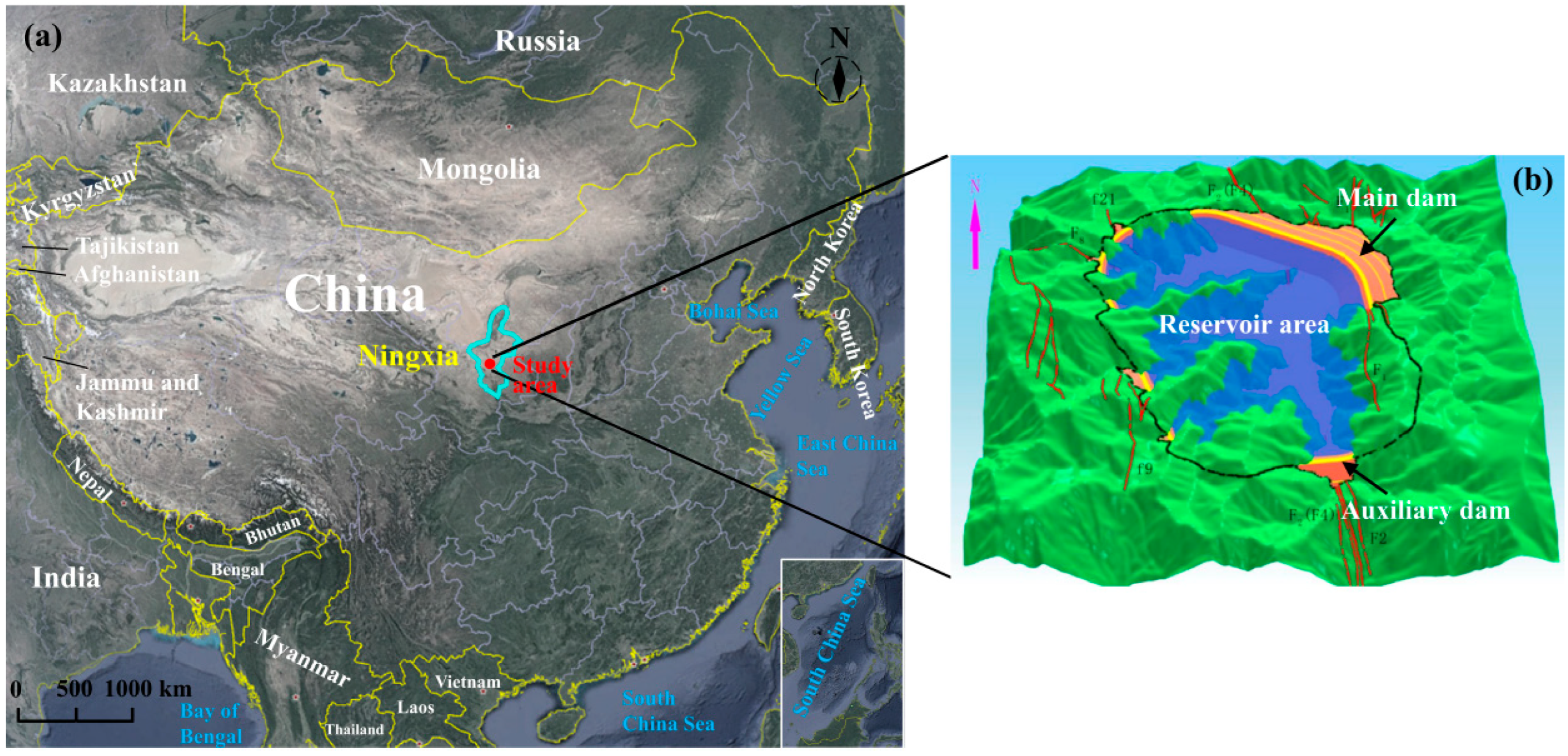
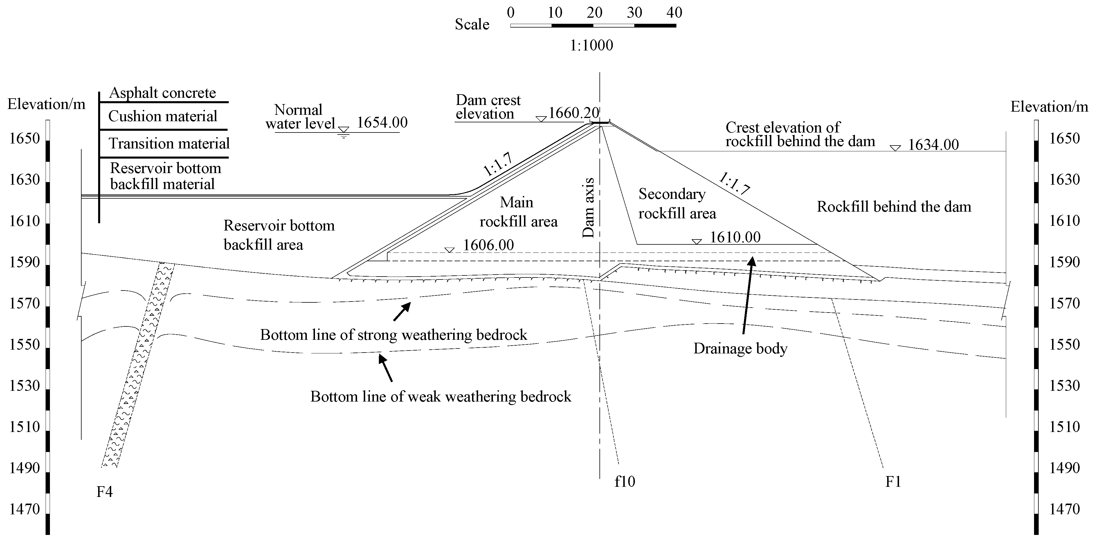
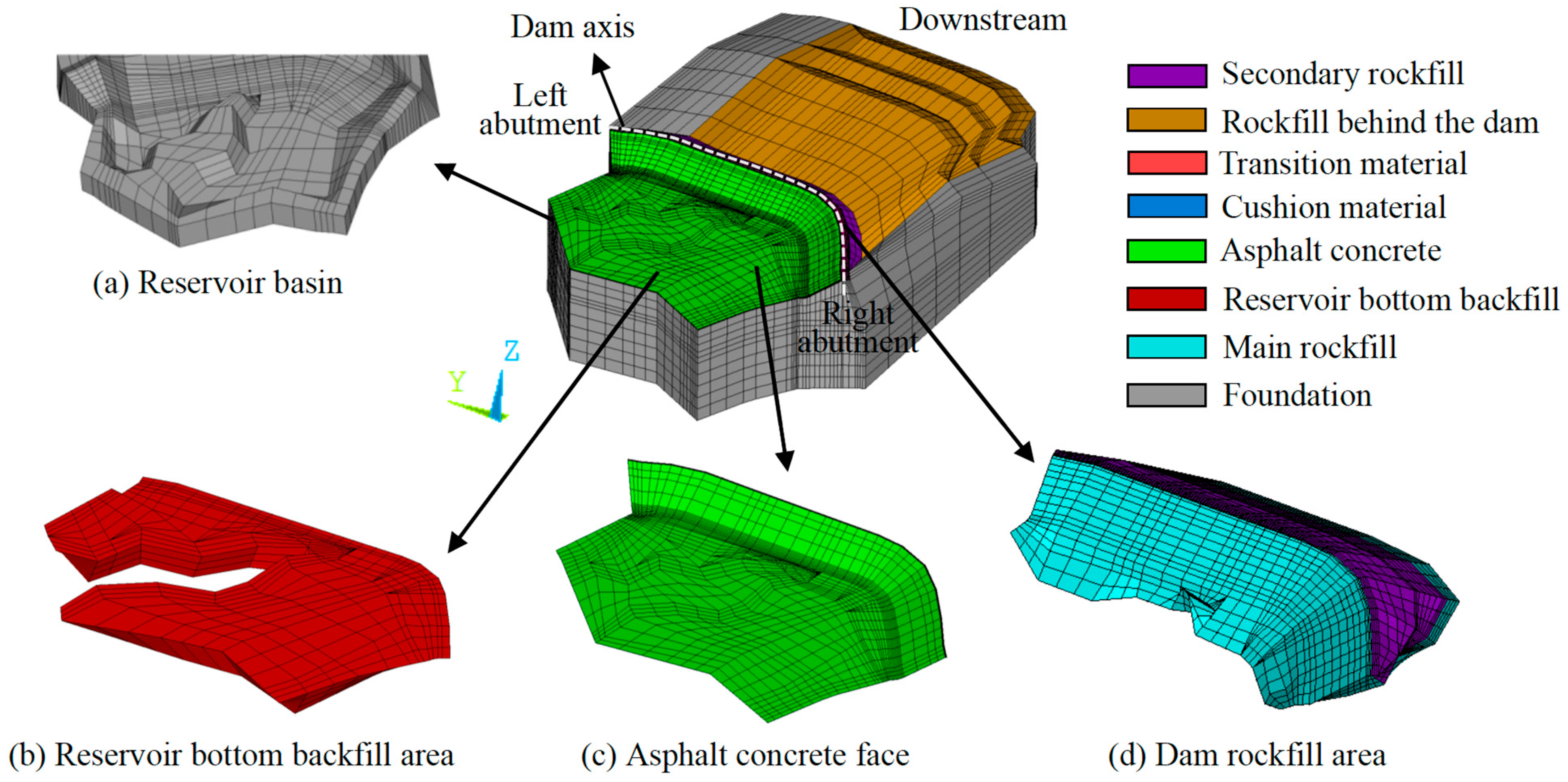
This research aimed to study the sensitivity of horizontal displacement of dam H, vertical displacement u, and asphalt concrete face tensile strain ε to model parameters in the analysis of PSPS dams and asphalt concrete face deformation with the Duncan–Chang E-B model. In this study, the ACFRD of a PSPS in Ningxia Province of China was taken as an example. According to the hydro-geological conditions and engineering design data of the project, a 3D finite element model of the dam’s deformation based on the Duncan–Chang E-B model was established. The orthogonal test was adopted. The sensitivity of PSPS’s ACFRD horizontal displacement H, vertical displacement u, and asphalt concrete face tensile strain ε to the main rockfill zone, secondary rockfill zone, and reservoir bottom backfill zone were studied to provide a theoretical basis for the selection of model parameters for PSPS’s ACFRD deformation analysis.

2. Duncan–Chang E-B Model

To calculate the deformation, the Duncan–Chang E-B model [45] was used to simulate the stress-strain characteristics of the soil. The stress-strain relationship of materials to the Duncan–Chang E-B model was usually obtained by experimental or field triaxial compression tests, which could be approximated as a hyperbola. The Duncan–Chang E-B model could be expressed as follows:
E t = E i ( 1 R f S ) 2
where Et is the tangential elastic modulus; Ei is the initial shear modulus; S is the stress level, which reflects the ratio of practical principal stress difference and principal stress difference at failure; Rf is the damage ratio, which is the ratio of principal stress difference asymptotic value to the actual failure principal stress difference; it was less than 1.0.
S = ( σ 1 σ 3 ) ( σ 1 σ 3 ) f
where σ1 is the maximum principal stress and σ3 is the minimum principal stress.
E i = K P a ( σ 3 P a ) n
where K and n are the initial elastic modulus base, and elastic modulus index, respectively, which are experimentally determined; Pa is the normal atmospheric pressure.
According to the Mohr-Coulomb fracture criterion [46,47]
( σ 1 σ 3 ) f = 2 C cos φ + 2 σ 3 sin φ 1 sin φ
where C is the cohesion and φ is the internal friction angle.
By inserting Equations (2)–(4) into Equation (1), the expression of the tangential modulus could be obtained:
E t = K P a ( σ 3 P a ) n [ 1 R f ( 1 sin φ ) ( σ 1 σ 3 ) 2 C cos φ + 2 σ 3 sin φ ] 2
The tangential bulk modulus could be calculated by
K t = K b P a ( σ 3 P a ) m
where Kb and m are initial bulk modulus base and bulk modulus index, respectively.
The elastic module of the material under unloading or reloading could be expressed as [24]
E u r = K u r P a ( σ 3 P a ) n u r
where Kur and nur were the elastic modulus base and elastic modulus index under unloading and reloading separately, respectively.
The Mohr envelope of the coarse aggregate showed obvious nonlinearity. The internal friction angle φ varied with the value of confining pressure σ3. Therefore, the internal friction angle could be calculated by the following formula:
φ = φ 0 Δ φ log ( σ 3 P a )
where φ0 is the initial internal friction angle; Δφ is the reduction value of friction angle φ when the confining pressure increases by one logarithmic period.
Hence, the Duncan–Chang E-B model parameters used to describe the nonlinear constitutive relationship of dam or reservoir bottom filling materials mainly include C, φ, Δφ, Rf, K, Kb, n, m, Kur, and nur. It should be noted that the creep properties of rockfill, asphalt, concrete, and overburden were simulated by a viscous-elastic-plastic model [48,49].

3. Orthogonal Test Method

3.1. Principle of Orthogonal Test Design

Orthogonal test design is a design method based on mathematical statistics and the orthogonality principle to select representative points from many test points. An orthogonal table is used to arrange and analyze multi-factor tests. Because of the characteristics of the “neat comparability” and “balanced dispersion” of the orthogonal table, using this method can effectively reduce the number of design tests and reflect the variation law of objective things.
An orthogonal table is key to the design of an orthogonal test. It is required to satisfy the following two conditions [43,44]: uniformity was ensured by the same occurrence of different levels of each column (factor); number pairs composed of different level combinations of any two columns (factors) have the same number of occurrences in the test, so as to ensure the uniformity of the distribution of test points. Only when the two conditions are satisfied can the test results be conveniently and comprehensively reflected. In orthogonal tests, the investigated results are called indicators, the parameters that may have an impact on the test indicators are called factors, and the specific test conditions for each factor to be compared in the test are called levels. The orthogonal table can be represented by the symbol Ln (rc). L is the code of the orthogonal table; n is the total number of tests; r is the level number of factors; c is the column number of the orthogonal table, that is, the maximum number of factors that can be arranged. Taking a test with seven factors and three levels as an example, the constructed orthogonal table is shown in Table 1. In Table 1, the first column of factors are two levels, and the last seven factors are three levels; the total number of tests is 18.

3.2. Analysis of Orthogonal Test

The orthogonal test results can be analyzed by: (a) range analysis and (b) variance analysis.

3.2.1. Range Analysis Method

In the range analysis method, the sensitivity degree of the factor is judged by range value Rj, which is defined as the influence degree of the change of the factor level on the test indicator. The greater the range, the greater the influence of the change of the factor level on the test index [50]. The range value is obtained by statistical Kij of factors under various levels. The basic principle of the range analysis method can be described as follows [50]:
K i j = 1 P i j k = 1 P i j Y k Y ¯
R j = Max { K 1 j ,   K 2 j , } Min { K 1 j ,   K 2 j , }
where Kij is the average value of the factor j under level i; Pij is the test numbers of factor j under level i; Yk is the indicator number of the kth test; Y ¯ is the average value of all test results.

3.2.2. Analysis of Variance (ANOVA) Method

Range analysis can intuitively reflect the sensitivity order of each factor, but it cannot distinguish whether the fluctuation of test results is caused by the change of factor level or by test error, and there is no clear boundary standard to determine whether the factor is sensitive. Therefore, to distinguish the influence of factor level change and test error and clearly point out the sensitivity degree of the factor, and to further compare and verify the results of range analysis, the variance analysis method was adopted in this study to analyze the test results. The basic principle of the variance analysis method is as follows.
Suppose that Ln (rc) is used to arrange the test, and the results of the kth test are recorded as Yk (k = 1, 2, ···n), the sum of the test results Yk of the ith level of the jth factor is represented as Tij, where T represents the sum of the total test results and pij is the number of tests of factor j under the ith level, then [44]:
T i j = k = 1 p i j Y k
T = k = 1 n Y k
Y ¯ = T 2 n
p i j = n r
The total variance of n test results was recorded as ST, indicating the degree of difference between all test results; the quadratic sum of the variance of the jth column was recorded as Sj, indicating the degree of difference between different levels of the factors listed in column j; the sum was marked as Se, indicating the different degree of test conditions during the test. The calculation formula could be expressed as [44]:
S T = k = 1 n Y k 2 Y ¯
S j = k = 1 r T i j p i j Y ¯
S e = S T j = 1 c S j
The degrees of freedom of ST, Sj, and Se were assumed to be ST, Sj, and Se, respectively, then:
f T = n 1
f j = r 1
f e = f T j = 1 c f j
In the calculation, the test results (Y1, Y2, ···Yn) were independent and obeyed the normal distribution with the same variance σ2. The statistics of the F test could be constructed [44]:
F j = S j / f j S e / f e ~ F ( f j , f e )
By comparing Fj with the critical test value, Fα (fj, fe) was found in the F distribution table. The sensitivity of the model output results to the changes of various factors could be judged.

4. Case Study

4.1. Study Site

The asphalt concrete face rockfill dam project of PSPS in this study was located at the western foot of the Niushou mountain on the right bank of the reservoir of the Qingtong gorge on the Yellow River in Ningxia, China. The upper reservoir of the PSPS is located in eastern Daxitian, the main peak of the Niushou mountain. The gully is in a “U” shape. The gully in the reservoir area is developed, and the bottom of the reservoir alternates ditches and beams. The gully needed to be backfilled with excavated materials from the reservoir basin to ensure that the reservoir bottom was flat; therefore, the foundation stiffness of the intense weathering rock mass and the weak weathering rock mass of the reservoir basin foundation and that of the backfilled and excavation area were quite different. The obvious foundation heterogeneity is prone to cause uneven deformation of the foundation. The reservoir bottom elevation of the upper reservoir of the PSPS is 1624 m; the normal water and dead water levels are 1654.00 and 1625.00 m, respectively; the maximum drawdown depth of the reservoir is 29 m; and the regulating reservoir capacity is 7.108 million m3, which is a daily regulating reservoir. The pivotal buildings of the project include ACFRD, reservoir basin anti-seepage system, and water inlet and outlet systems. According to the relevant provisions of “Standards for Classification of Hydro-power Projects and Design Safety” (DL5180-2003) and “Standards for Flood Control” (GB50201-2014) in China, this project is a second-class (2) type project according to its storage capacity. The construction of the reservoir was of great significance to the development of the local economy and electrical equipment. Figure 1 shows the geographical location and layout of the reservoir site.
The maximum dam height of the main dam in the project is 78 m with a crest elevation of 1660.2 m; the maximum depth of the reservoir bottom backfill zone is 38 m; the crest length is 549.80 m; the crest width is 10 m; the dam slope ratios of upstream and downstream are all 1:1.7. The zone of the dam from upstream to downstream can be divided into the cushion zone (thickness = 3 m), transition zone (thickness = 3 m), main rockfill zone, secondary rockfill zone, and rockfill behind the dam.
The asphalt concrete face with a simple section structure was adopted for seepage prevention in the reservoir basin. The thickness of the panel is 0.202 m. From top to bottom, there is a 2 mm thick asphalt mastic sealing layer, 10 cm thick asphalt concrete anti-seepage layer, and 10 cm thick flat cementation layer. The reservoir bottom and dam are connected by a thickened asphalt concrete arc. The cementation layer was laid between the gravel drainage cushion and the anti-seepage layer to ensure the stable combination of the asphalt concrete face and the cushion. A typical section of the dam along the river is shown in Figure 2.

4.2. Establishment of Finite Element Model

The actual deformation generally occurred in the semi-infinite domain below the ground, and the deformation calculation could only be conducted in a limited region; therefore, it was very important to determine the scope of the calculation domain for model generalization. The bottom and sides of the deformation calculation domain were truncated boundaries, which were often difficult to accurately determine. Therefore, in addition to including the design area concerned with the displacement field in the computational domain, the position of the truncation boundary should be taken as a position where the error of the adopted boundary conditions has little influence on the displacement field of the concerned area.
In view of the aforementioned principles, the calculation coordinate system and model interception range were defined as follows: the x direction of the model was perpendicular to the dam axis with the positive direction pointing downstream; the y direction was along the dam axis with the positive direction pointing to the left bank; the z-axis was vertically upward with the elevation as the coordinate. The truncated boundaries were 40 m outside the left dam abutment and 60 m outside the right dam abutment. The scope of the reservoir was 20 m within the main backfill area. The downstream truncated boundary was 2 m outside any material area behind the dam. The top elevation was taken as the actual terrain, and the bottom elevation was 1624 m.
According to the geological structure of the dam foundation and abutment on both banks, as well as the requirements of layered filling and loading, super element automatic or manual dissection was adopted to form the finite element mesh. The element model mesh had 20,207 nodes and 20,185 elements after discretization by the hexahedral cells. The nodes and elements for the asphalt concrete face are 1308 and 1244, respectively, and the maximum and minimum sizes are 10.6 m and 0.55 m, respectively. The three-dimensional finite element mesh of the computational zone is shown in Figure 3. It should be noted that in the subsequent description, the dam body refers to the combination of Figure 3b,d.

4.3. Model Parameters

During model calculation, the dam foundation overburden, dam material (e.g., asphalt concrete face, cushion, transition layer, main rockfill zone, secondary rockfill zone), reservoir bottom backfill zone, and rockfill behind the dam were all considered nonlinear materials [51,52]. The Duncan–Chang E-B model was used to describe the nonlinear constitutive relationship of materials. The calculation parameters are shown in Table 2. Both preventative water-wave concrete walls and bedrock were considered linear materials. A linear elastic model was used to describe the constitutive relationship of materials. The calculation parameters are shown in Table 3. All calculation parameters in this study were provided by the design department and geological exploration department of the project.
It should be noted that the calculation parameters were obtained according to Chinese national industry standards. For instance, geotechnical parameters were obtained through laboratory tests in accordance with the “Standard for Geotechnical Testing Method in China” (GB/T 50123-2019), and asphalt concrete parameters were obtained through laboratory tests in accordance with the “Standard for Test Code for Hydraulic Bitumen Concrete in China” (DL/T 5362-2006).

4.4. Boundary Conditions and Step Loading

For boundary conditions, the bottom boundary of the model was a fixed constraint boundary, and the surrounding truncated boundary was constrained in the x and y directions. The purpose of staged loading was mainly to simulate the construction process and water storage process of the dam, reservoir bottom backfill, rockfill behind the dam, and asphalt concrete face. In staged loading, the mountains around the reservoir basin were loaded first, and then the geo-stress balance was conducted. Before loading the reservoir bottom backfill and dam materials, the node displacement was reset to zero, and the element stress was reserved to obtain the initial stress field of the foundation. The calculated displacements were all caused by construction. The whole dam construction and water storage process was divided into 24 levels, as shown in Figure 4. Each level of the load was loaded once, and the midpoint increment method was used to better simulate the loading process.

4.5. Deformation Analysis Based on the Established Model

4.5.1. Horizontal Displacement of Dam Rockfill

Based on the proposed finite element model, the dam rockfill horizontal displacement distribution along the valley direction after completion and impoundment periods (as shown in Figure 5) were calculated. Notably, the horizontal displacement was positive to point to the downstream direction and negative to point to the upstream direction along the river valley. As shown in Figure 5a, after completion, limited by topographic conditions, the maximum horizontal displacement of the dam rockfill downstream along the valley appeared at the middle ridge of the main rockfill zone ((x, y, z) = (−32.2, 59.1, 1640.1)), and the maximum displacement was about 42.17 mm. The maximum displacement of the dam rockfill upstream along the valley was about 68.26 mm, which occurred at the main rockfill zone ((x, y, z) = (−48.6, 213.1, 1606.7)). The maximum displacement of the reservoir bottom backfill zone downstream along the valley was 39.4 mm, which appeared at (x, y, z) = (−324.1, −42.6, 1618.5).
As shown in Figure 5b, after impoundment, the displacement of the dam rockfill zone downstream increased, and the maximum displacement was about 96.03 mm, which appeared at the main rockfill zone ((x, y, z) = (−40.6, 75.0, 1635.2)). The maximum displacement of the dam rockfill zone upstream was about 37.38 mm and appeared at the dam crest ((x, y, z) = (7.32, 271.4, 1650.6)). The maximum displacement of the reservoir bottom backfill zone upstream was about 71.42 mm, which appeared at (x, y, z) = (−242.3, 162.6, 1618.5). The maximum displacement of the reservoir bottom backfill zone downstream was 87.58 mm, which appeared at (x, y, z) = (−158.6, 169.5, 1618.5).
According to the results of the typical cross-section displacement along the river valley, the reservoir bottom backfill zone had an impact on the main rockfill displacement. The maximum displacement of the typical surface to the upstream appeared near y = −30 m, and the displacement at this position decreased under the action of water pressure after impounding. Moreover, after completion, the displacement change of the reservoir bottom surface of the typical section was small, and there was a certain displacement difference on the dam slope. However, after impounding, the displacement difference on the reservoir bottom surface increased to about 60 mm. Although the displacement of the dam slope along the river increased after impounding, the displacement difference was not much different from after completion.

4.5.2. Vertical Displacement of Dam Rockfill

Figure 6 shows the distribution of vertical displacements of dam rockfill after completion and impoundment. Notably, vertical displacement was positive when it was vertically upward and negative when it was vertically downward. As observed, after completion, the maximum vertical displacement of the dam rockfill (506.3 mm) occurred at the dam abutments on both banks of the main rockfill zone ((x, y, z) = (3.2, 109.4, 1622.2)). The maximum vertical displacement of the reservoir bottom backfill zone appeared in the center of the reservoir basin ((x, y, z) = (−253.1, −8.2, 1606.9)). After impoundment, the maximum vertical displacement of the dam rockfill was 525.1 mm, which appeared at about half the dam’s height of the main rockfill zone ((x, y, z) = (−5.8, 109.4, 1622.2)). This was consistent with the actual general law, proving the reliability of the proposed model. Based on the maximum dam height (= 78 m), the maximum vertical displacement was about 0.673% of the maximum dam height. The maximum vertical displacement of the reservoir bottom backfill zone was about 493.4 mm, which appeared at (x, y, z) = (−261.5, 37.3, 1614.7). Based on the maximum depth of the reservoir bottom backfill zone = 38 m, the maximum vertical displacement accounted for about 1.3%.
According to the vertical displacement results of typical cross sections, after completion, the maximum vertical displacement of the dam rockfill was 505.1 mm at (x, z) = (−3.5, 1622.2), and the maximum vertical displacement of the reservoir bottom backfill was 276.8 mm at z = 1607 m. After impoundment, the maximum vertical displacement of the dam rockfill was 523 mm at (x, z) = (−11.9, 1622.2), and the maximum vertical displacement of the reservoir bottom backfill was 496.9 mm at z = 1615 m.

4.5.3. Tensile Strain of Asphalt Concrete Face

From a safety point of view, the internal structure of the anti-seepage material cannot be damaged. In terms of the safety of stress-strain curves of asphalt concrete, the linear section was generally regarded as the main working stage of asphalt concrete. According to the relevant provisions of “Standards for Design Code of Asphalt Concrete Facings and Cores for Embankment Dams” (SL 501-2010), the content of asphalt in the impervious layer of asphalt concrete face could be from 6.5–8.5%. According to much triaxial test data, if the stress when the volume changed from compression equilibrium to micro-expansion was regarded as failure stress [53], the tensile range of the asphalt concrete was 1.0~1.3 MPa. The test value of yield tensile strain for the asphalt concrete at 5 °C at the Sabigawa Dam, Japan at 0.5%. The allowable tensile strain of the modified asphalt concrete could reach 1%, but 0.5% was taken as the yield tensile strain for the asphalt concrete in engineering practice. Figure 7 shows the distribution of tensile strain of asphalt concrete face after impoundment. It should be noted that the negative value represents tensile strain, and the positive represents compressive. To clearly show the tensile strain, strain values above 0 were uniformly limited to one level here, i.e., the compressive strain is displayed in blue.
As shown in Figure 7, the tensile strain peak area appeared at the reverse arc section of the panel and the excavation-filling interface. Overall, the tensile strain of the reverse arc section of the panel was larger at the reservoir bottom backfill zone and tended to gradually decrease towards the middle ridge and the two banks. The tensile strain of most of the panel reverse arc section of the reservoir bottom backfill zone exceeded 0.3%, but the maximum tensile strain was only 0.445%, which did not exceed the specification value by 0.5%, so it was safe. For the excavation-filling interface, the maximum tensile strain was 0.483%, which did not exceed the allowable value of 0.5%. The tensile strain at other locations was not more than 0.05%. It is slightly larger at the left and right bank abutments but still within the allowable range of the specification value. Therefore, the whole asphalt concrete face was safe after impoundment.

4.6. Sensitivity Analysis

4.6.1. Orthogonal Test Design and Results

There were 10 parameters involved in the Duncan–Chang E-B model, including: K, n, Rf, φ, Δφ, Kb, m, c, Kur, and nur. In the process of filling and impounding, the rockfill zone was under a loading state. Parameters Kur and nur were not included in the calculation, and the rockfill was a granular material, so parameter c could be considered zero. Therefore, the factors for sensitivity analysis were φ0, Δφ, Rf, K, n, Kb, and m.
Under the self-weight of the rockfill and water load, vertical and horizontal deformation upstream and downstream had a great impact on the dam. At the same time, considering that the excessive asphalt concrete face tensile strain was the main cause of panel cracking, the dam maximum vertical displacement u, maximum horizontal displacement H, and asphalt concrete face tensile strain ε were selected as the main test indices of parameter sensitivity analysis. Based on the above model calculation parameters, the basic parameters were increased or decreased by 20% as the three level values of the orthogonal test in this study. Table 4 shows the levels of various factors adopted in the orthogonal test sensitivity analysis.
According to the test factors and levels, the L18 (2 × 37) orthogonal table was selected in this study. The first column in the table was set as empty and was not included in the calculation and analysis. The different levels of each factor were filled in accordingly. Assuming that the test factors were independent, the corresponding orthogonal table could be obtained by randomly filling the test factors in the last seven columns of the orthogonal table. Considering the possible differences in the sensitivity of test indicators to model parameters in different zones, the main rockfill, secondary rockfill, and reservoir bottom backfill zones were separately considered, and the maximum vertical displacement of the dam u, maximum horizontal displacement H, and tensile strain of asphalt concrete ε during the impoundment period under the orthogonal combination of the Duncan–Chang E-B model parameters of these three zones was calculated. The test scheme and results are shown in Table 5, Table 6 and Table 7.

4.6.2. Sensitivity Analysis Based on Range Analysis Method

Range Analysis for Main Rockfill Zone

The range analysis method was used to process the results of each scheme in the three columns u, H, and ε and in the summary table of orthogonal test results in the main rockfill zone (Table 5). The range analysis results are shown in Table 8.
The range analysis results of each test index u, H, and ε in the main rockfill zone were organized, and then the range value histogram was drawn according to the range value of each test index according to each factor, as shown in Figure 8.
As shown in Table 8 and Figure 8, during the impoundment period, the sensitivity degree of maximum vertical displacement of dam u to indices of the Duncan–Chang E-B model of the main rockfill zone from high to low was Rf > φ0 > K > Kb > n > Δφ > m; the sensitivity of maximum horizontal displacement H to indices of the Duncan–Chang E-B model of main rockfill zone from high to low was Kb > Rf > K > φ0 > n > m > Δφ; the sensitivity of asphalt concrete face maximum tensile strain ε to indices of the Duncan–Chang E-B model of main rockfill zone from high to low was Kb > Rf > φ0 > K > n > m > Δφ.

Range Analysis for Secondary Rockfill Zone

The range analysis method was used to process the results of each scheme in the three columns u, H, and ε in the summary table of the orthogonal test results in the secondary rockfill zone (Table 6). The range analysis results are shown in Table 9.
The range analysis results of each test index u, H, and ε in the secondary rockfill zone were sorted out, and then the range value histogram was drawn according to the range value of each test index according to each factor, as shown in Figure 9.
As shown in Table 9 and Figure 9, during the impoundment period, the sensitivity degree of maximum vertical displacement of dam u to indexes of secondary rockfill zone Duncan–Chang E-B model from high to low was Kb > K > Rf > φ0 > Δφ > m > n; the sensitivity of maximum horizontal displacement H to indexes of Duncan–Chang E-B model of secondary rockfill zone from high to low was Kb > Rf > K > φ0 > Δφ > m > n; the sensitivity of maximum tensile strain of asphalt concrete face ε to indexes of Duncan–Chang E-B model of secondary rockfill zone from high to low was Kb > K > φ0 > m > Δφ > n > Rf.

Range Analysis for Reservoir Bottom Backfill Zone

The range analysis method was used to process the results of each scheme in the three columns of u, H, and ε in the summary table of orthogonal test results in the reservoir bottom backfill zone (Table 7), and the range analysis results were shown in Table 10.
The range analysis results of each test index u, H, and ε in the reservoir bottom rockfill zone were sorted out, and then the range value histogram was drawn according to the range value of each test index according to each factor, as shown in Figure 10.
As shown in Table 10 and Figure 10, during the impoundment period, the sensitivity of maximum vertical displacement of dam u to indexes of reservoir bottom backfill zone Duncan–Chang E-B model from high to low was Rf > K > Kb > n > φ0 > m > Δφ; the sensitivity of maximum horizontal displacement H to indexes of Duncan–Chang E-B model of reservoir bottom backfill zone from high to low was Kb > Rf > K > Δφ > φ0 > n > m; the sensitivity of maximum tensile strain of asphalt concrete face ε to indexes of Duncan–Chang E-B model of reservoir bottom backfill zone from high to low was Kb > Rf > K > φ0 > Δφ > n > m.

4.6.3. Sensitivity Analysis Based on ANOVA Method

For the variance analysis of the orthogonal test results, the test level confidences were selected α = 0.05 and α = 0.1. From the F distribution table, F0.05 (2, 3) = 16.0 and F0.1 (2, 3) = 5.46. The significance levels of the factors were judged by comparing the calculated Fj with the earlier values. The judgment criteria were when Fj > F0.05 (2, 3), the influence of this factor was highly significant, and the sensitivity was high; when F0.1 (2, 3) ≤ FjF0.05 (2, 3), the influence of this factor was generally significant, and the sensitivity was medium; and when Fj < F0.1 (2, 3), the influence of this factor was not significant, and the sensitivity was low.

ANOVA for Main Rockfill Zone

The results of each scheme involved u, H, and ε in the main rockfill zone orthogonal test results (Table 5) were analyzed with the variance analysis method, and the variance analysis results are shown in Table 11.
To reflect the results of the analysis, the ANOVA results for each test index were collated, and a sensitivity size bar chart was plotted from the F value of each test index (Figure 11). Notably, for comparison convenience, the influence value F of Kb and Rf on the test index H was reduced by 1.5 times, as seen in Figure 11.
As shown in Table 11 and Figure 11, for the maximum vertical displacement of dam u, the sensitivity degree of the Duncan–Chang E-B model of the main rockfill zone parameters from high to low was Rf > φ0 > K > Kb > n > Δφ > m. The influence of Rf was highly significant, and the sensitivity was high; the influences of φ0 and K were generally significant, and the sensitivities were medium; the influences of Kb, n, Δφ, and m were not significant, and the sensitivities were low. For the maximum horizontal displacement of dam H, the sensitivity degree of Duncan–Chang E-B model of main rockfill zone parameters from high to low was Kb > Rf > K > φ0 > n > m > Δφ. The influences of Kb, Rf, K, and φ were highly significant, and the sensitivities were high; the influences of n, m, and Δφ were not significant, and the sensitivities were low. For the tensile strain of asphalt concrete ε, the sensitivity degree of the Duncan–Chang E-B model of the main rockfill zone parameters from high to low was Kb > Rf > φ0 > K > n > m > Δφ. The influence of Kb was highly significant, and the sensitivity was high; the influence of Rf was generally significant, and the sensitivity was medium; the influences of φ0, K, n, m, and Δφ were not significant, and the sensitivities were low.

ANOVA for Secondary Rockfill Zone

The results of each scheme involved u, H, and ε in the secondary rockfill zone’s orthogonal test results (Table 6) were analyzed with the variance analysis method, and the variance analysis results are shown in Table 12.
To obviously reflect the results of the analysis, the ANOVA results for each test index were collated, and a sensitivity size bar chart was plotted through the F value of each test index (Figure 12). Notably, for comparison convenience, the influence value F of Kb on the test index u, H, and ε was reduced three times in Figure 12.
As shown in Table 12 and Figure 12, for the maximum vertical displacement of dam u, the sensitivity degree of the Duncan–Chang E-B model of the secondary rockfill zone parameters from high to low was Kb > K > Rf > φ0 > Δφ > m > n. The influences of Kb and K were highly significant, and the sensitivities were high; the influence of Rf was generally significant, and the sensitivity was medium; the influences of φ0, Δφ, m, and n were not significant, and the sensitivities were low. For the maximum horizontal displacement of dam H, the sensitivity degree of the Duncan–Chang E-B model of the secondary rockfill zone parameters from high to low was Kb > Rf > K > φ0 > Δφ > m > n. The influence of Kb was highly significant, and the sensitivity was high; the influences of Rf and K were generally significant, and the sensitivities were medium; the influences of φ0, Δφ, m, and n were not significant, and the sensitivities were low. For the tensile strain of asphalt concrete ε, the sensitivity degree of the Duncan–Chang E-B model of the secondary rockfill zone parameters from high to low was Kb > K > φ0 > m > Δφ > n > Rf. The influence of Kb was highly significant, and the sensitivity was high; the influences of K, φ0, m, Δφ, n, and Rf were not significant, and the sensitivities were low.

ANOVA for Reservoir Bottom Backfill Zone

The results of each scheme involved u, H, and ε in the reservoir bottom backfill zone orthogonal test results (Table 6) were analyzed with the variance analysis method, and the variance analysis results are shown in Table 13.
To obviously reflect the results of the analysis, the ANOVA results for each test index were collated, and a sensitivity size bar chart was plotted from the F value of each test index (Figure 13). Notably, for comparison convenience, the influence value F of Kb and m on the test index u was reduced ten times in Figure 13 and two times of Kb on the test index H.
As shown in Table 13 and Figure 13, for the maximum vertical displacement of dam u, the sensitivity degree of the Duncan–Chang E-B model of the reservoir bottom backfill zone parameters from high to low was Rf > K > Kb > n > φ0 > m > Δφ. The influences of Rf, K, and Kb were highly significant, and the sensitivities were high; the influences of φ0, n, and m were generally significant, and the sensitivities were medium; the influences of φ0, Δφ, m, and n were not significant, and the sensitivities were low. For the maximum horizontal displacement of dam H, the sensitivity degree of the Duncan–Chang E-B model of the reservoir bottom backfill zone parameters from high to low was Kb > Rf > K > Δφ > φ0 > n > m. The influences of Kb, K, and Rf were highly significant, and the sensitivities were high; the influences of Δφ and φ0 were generally significant, and the sensitivities were medium; the influence of n and m were not significant, and the sensitivities were low. For the tensile strain of asphalt concrete ε, the sensitivity degree of the Duncan–Chang E-B model of the reservoir bottom backfill zone parameters from high to low was Kb > Rf > K > φ0 > Δφ > n > m. The influence of Kb was highly significant, and the sensitivity was high; the influences of K, φ0, m, Δφ, n, and Rf were not significant, and the sensitivities were low.

4.6.4. Comparison of Sensitivity Results of Range Analysis and ANOVA

To explore the analysis accuracy of deformation-sensitive parameters of the PSPS asphalt concrete face dam with an orthogonal test, the results obtained by the range analysis and variance analysis methods were compared, as shown in Table 14. The results obtained by the variance analysis were consistent with those obtained by the range analysis, which reflected the rationality of the sensitivity analysis results in this study to some extent.

5. Conclusions

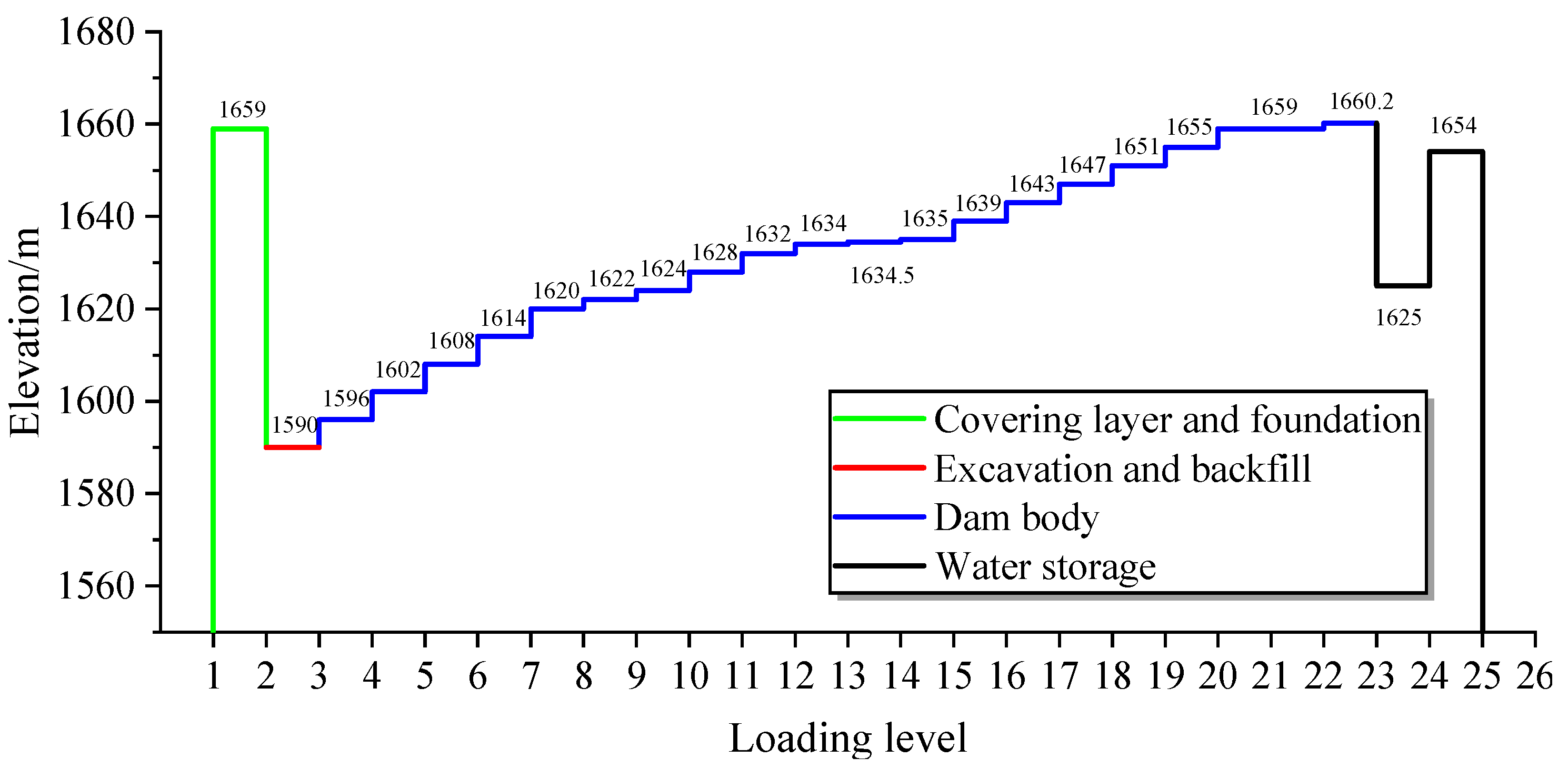
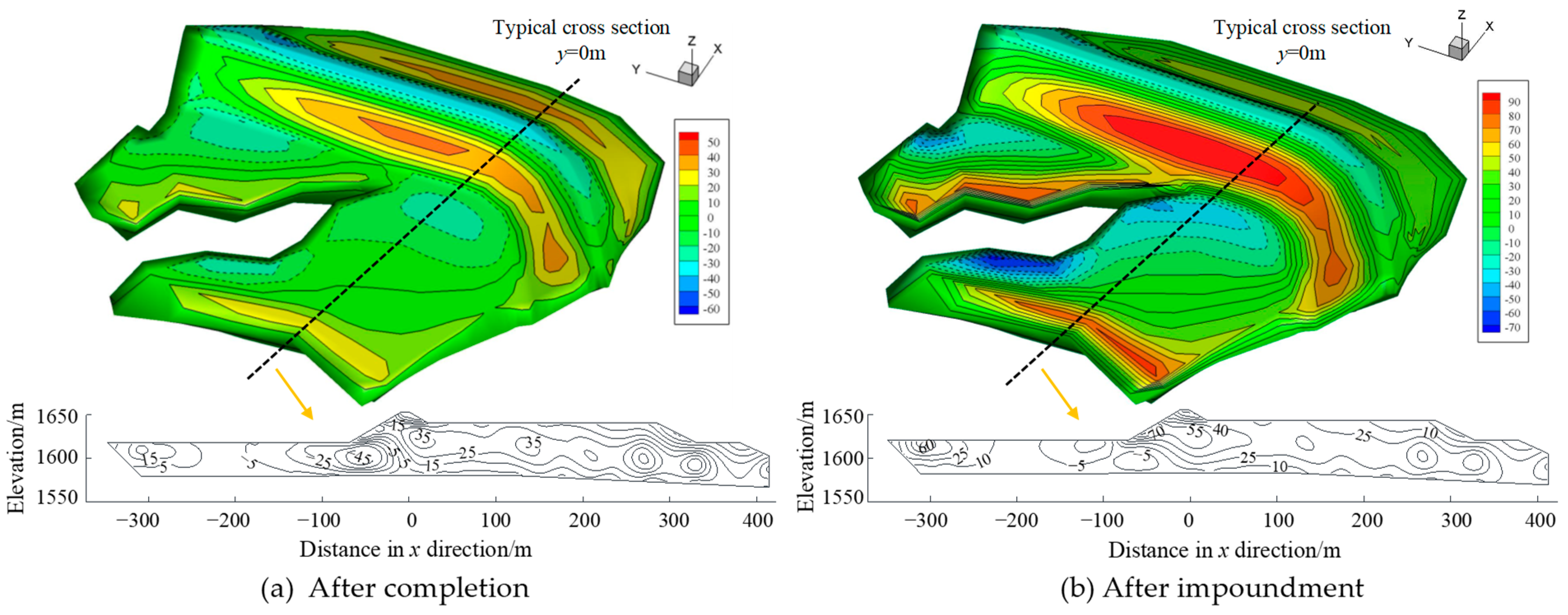
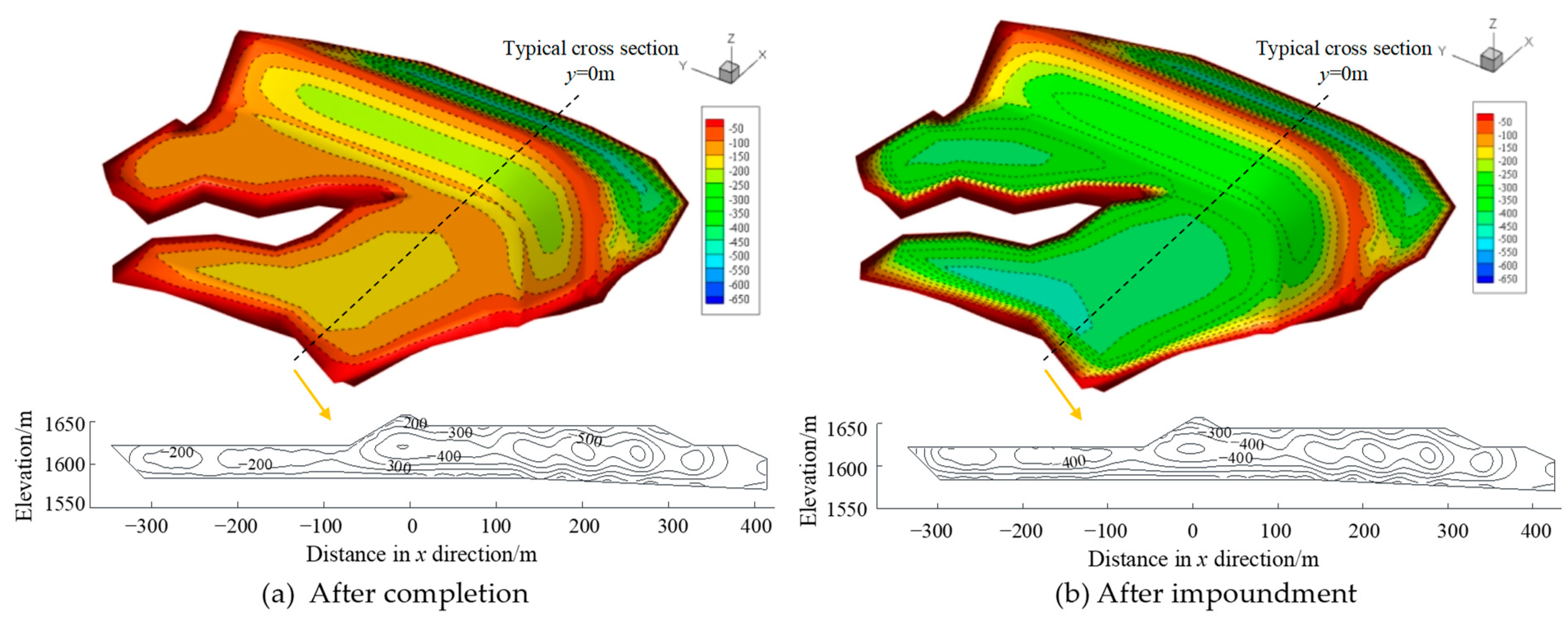
To determine the sensitivity of the deformation of the ACFRD of the PSPS to the Duncan–Chang E-B model parameters, a PSPS project in Ningxia, China, was taken as an example. Firstly, an ACFRD deformation finite element analysis model based on the Duncan–Chang E-B model was established, and the laws of dam horizontal displacement, vertical displacement, and asphalt concrete face tensile strain under the conditions of completion period and impoundment period were analyzed. Then, based on the orthogonal test, the sensitivities of ACFRD horizontal displacement, vertical displacement, and asphalt concrete face tensile strain to the Duncan–Chang E-B models of the main rockfill zone, secondary rockfill zone, and reservoir bottom backfill zone were studied. Finally, the results of the two orthogonal test sensitivity analysis methods (i.e., range analysis and ANOVA methods) were compared to demonstrate the rationality of the sensitivity analysis results. The major conclusions derived from this study could be summarized as follows:
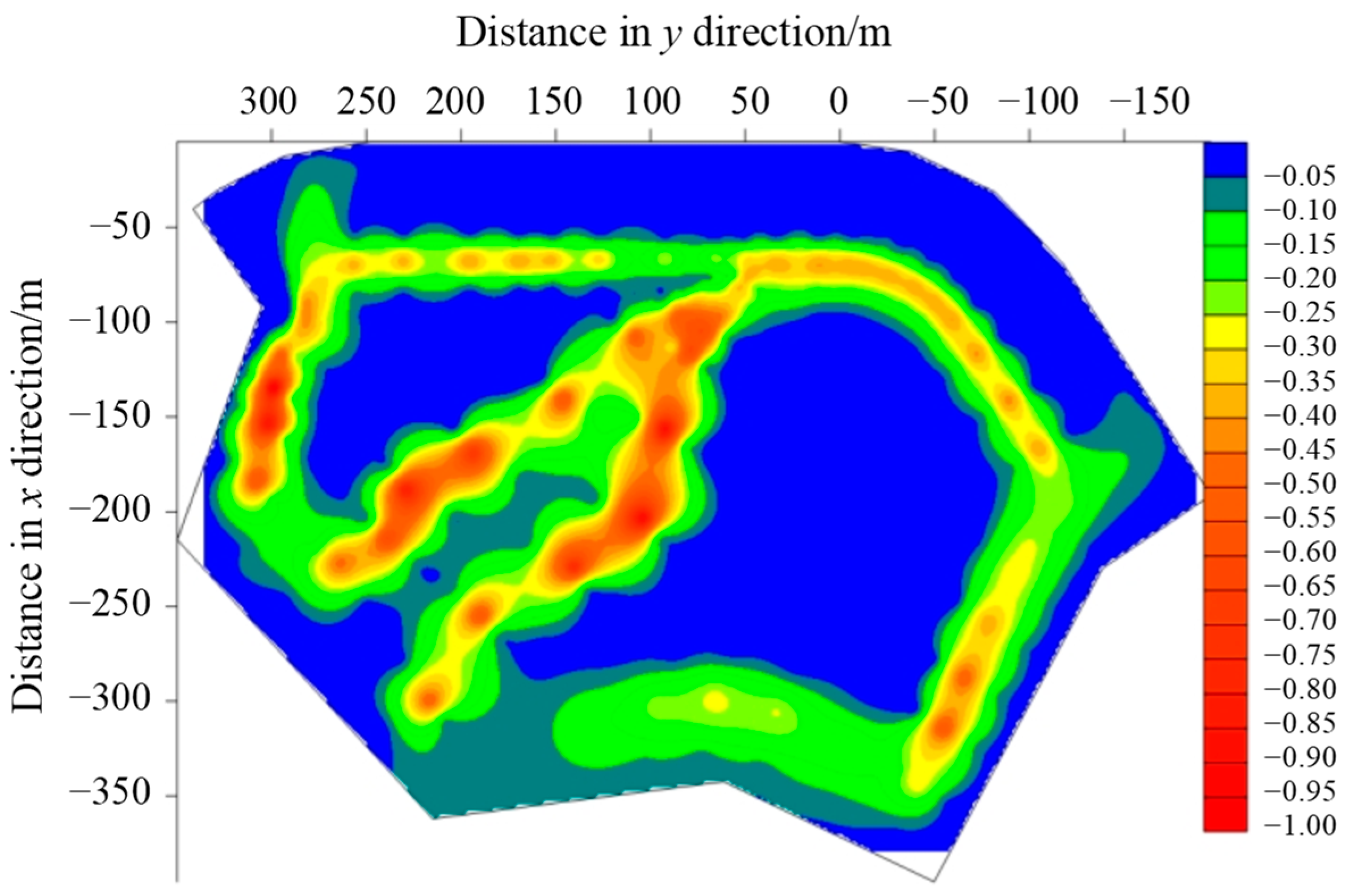
1. The PSPS’s ACFRD deformation finite element analysis model based on the Duncan–Chang E-B model could reasonably reflect the dam’s horizontal displacement, vertical displacement, and the tensile strain of the asphalt concrete face during the completion and impoundment periods. The maximum vertical displacement of the dam appeared at about half the dam’s height of the main rockfill zone in the impoundment period, which was consistent with the actual general law, indicating the rationality of the model calculation results. The maximum tensile strain of asphalt concrete face was 0.483%, which did not exceed the allowable value of 0.5% in the impoundment period. Therefore, during the operation of the dam, the asphalt concrete face was safe.
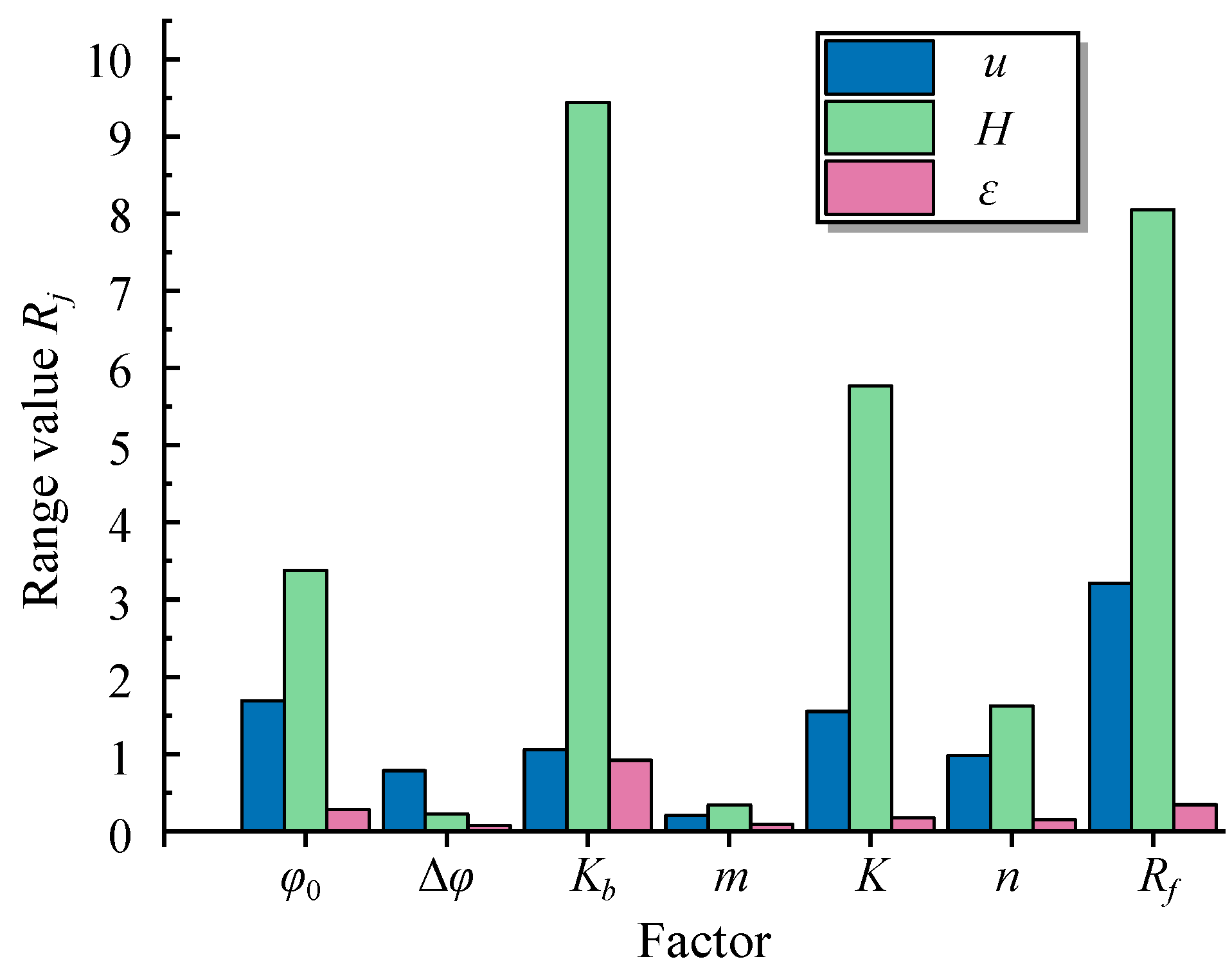
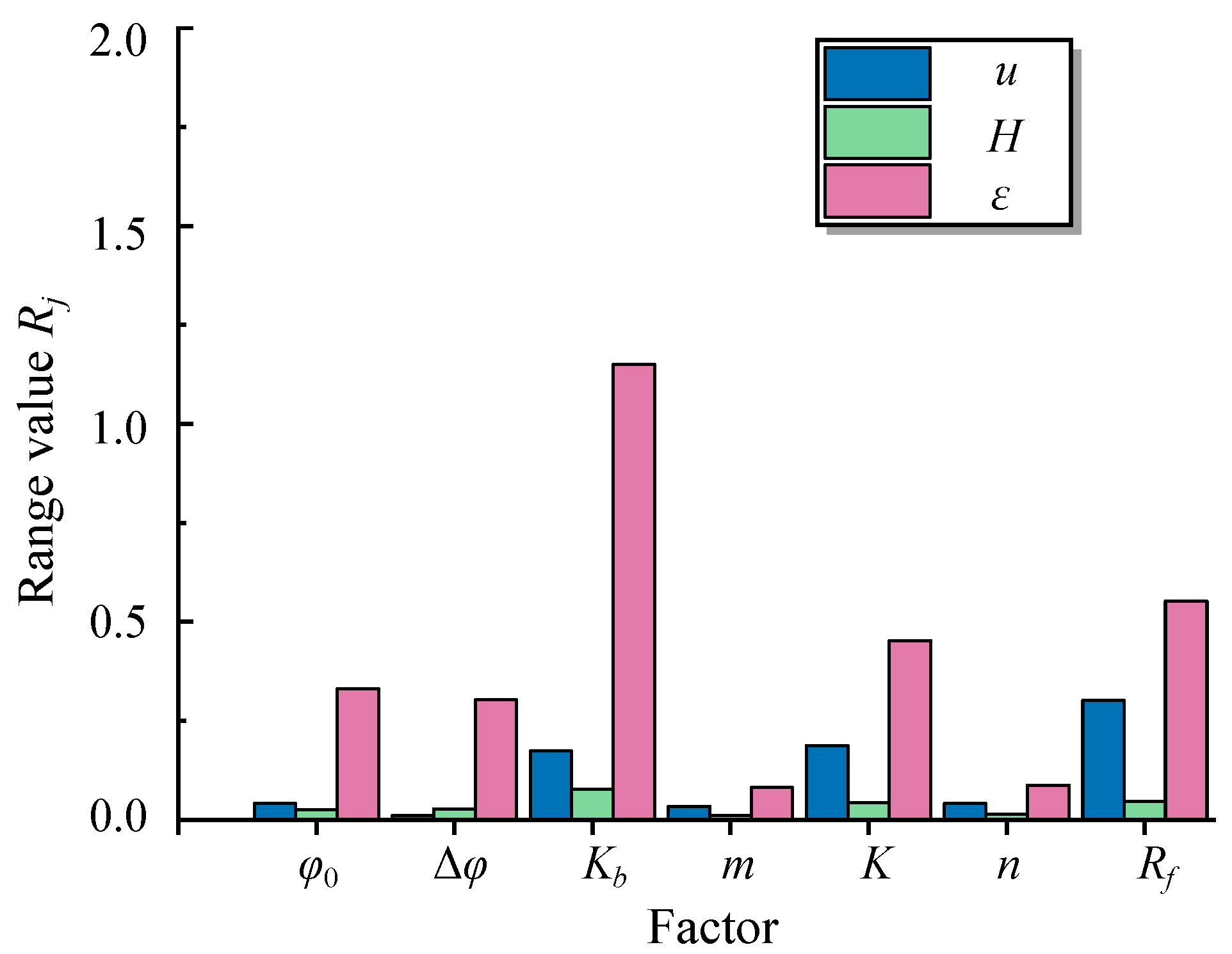
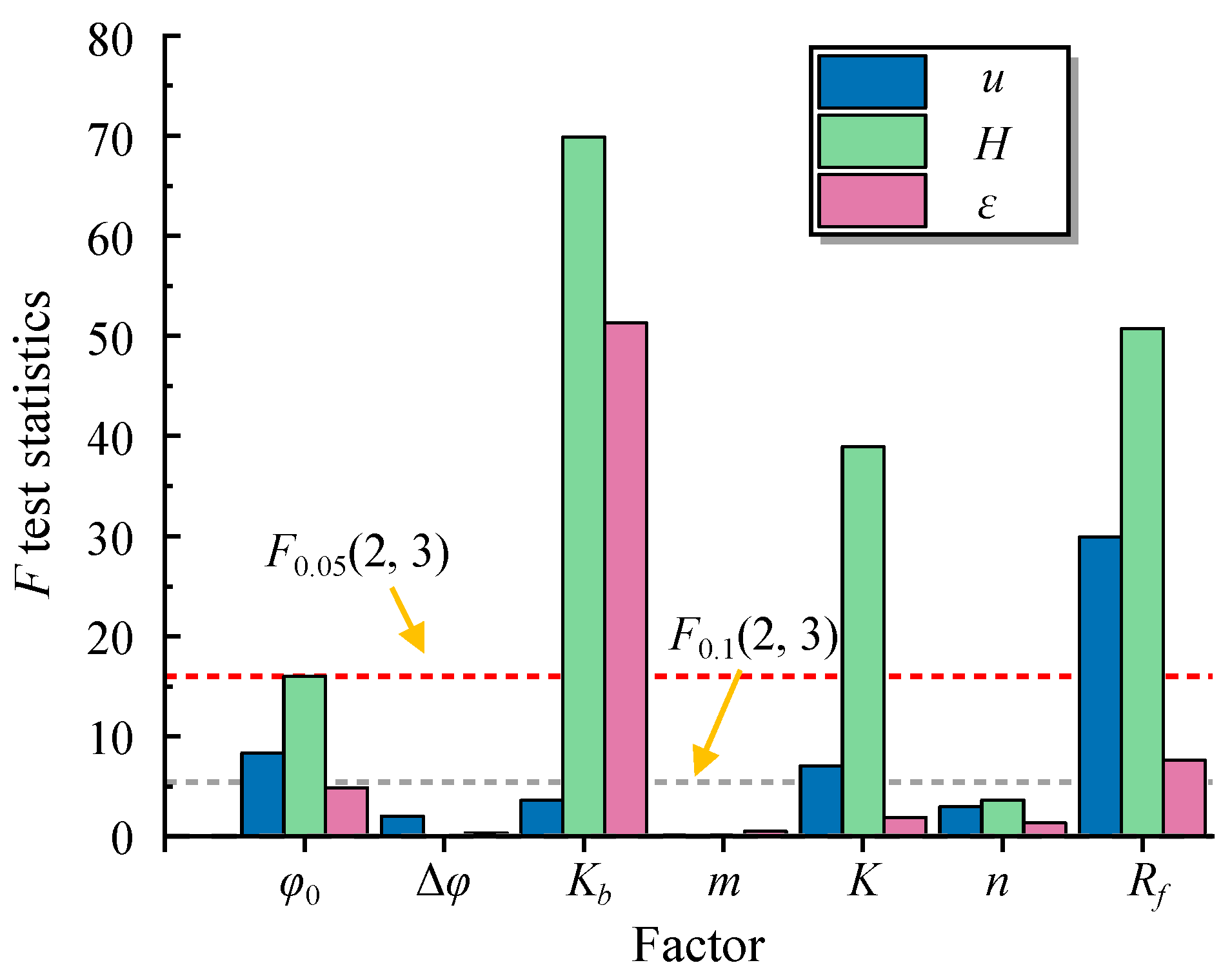
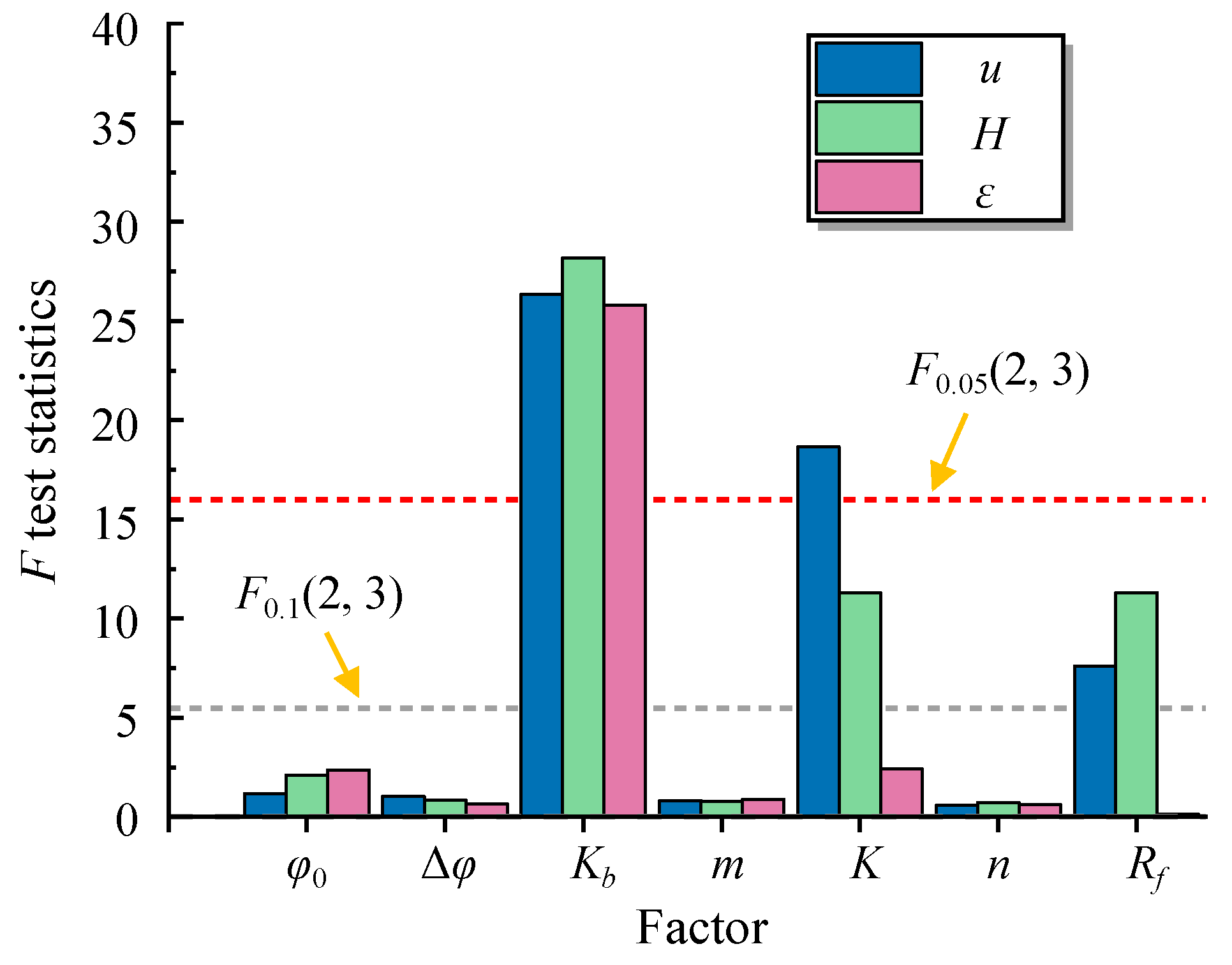
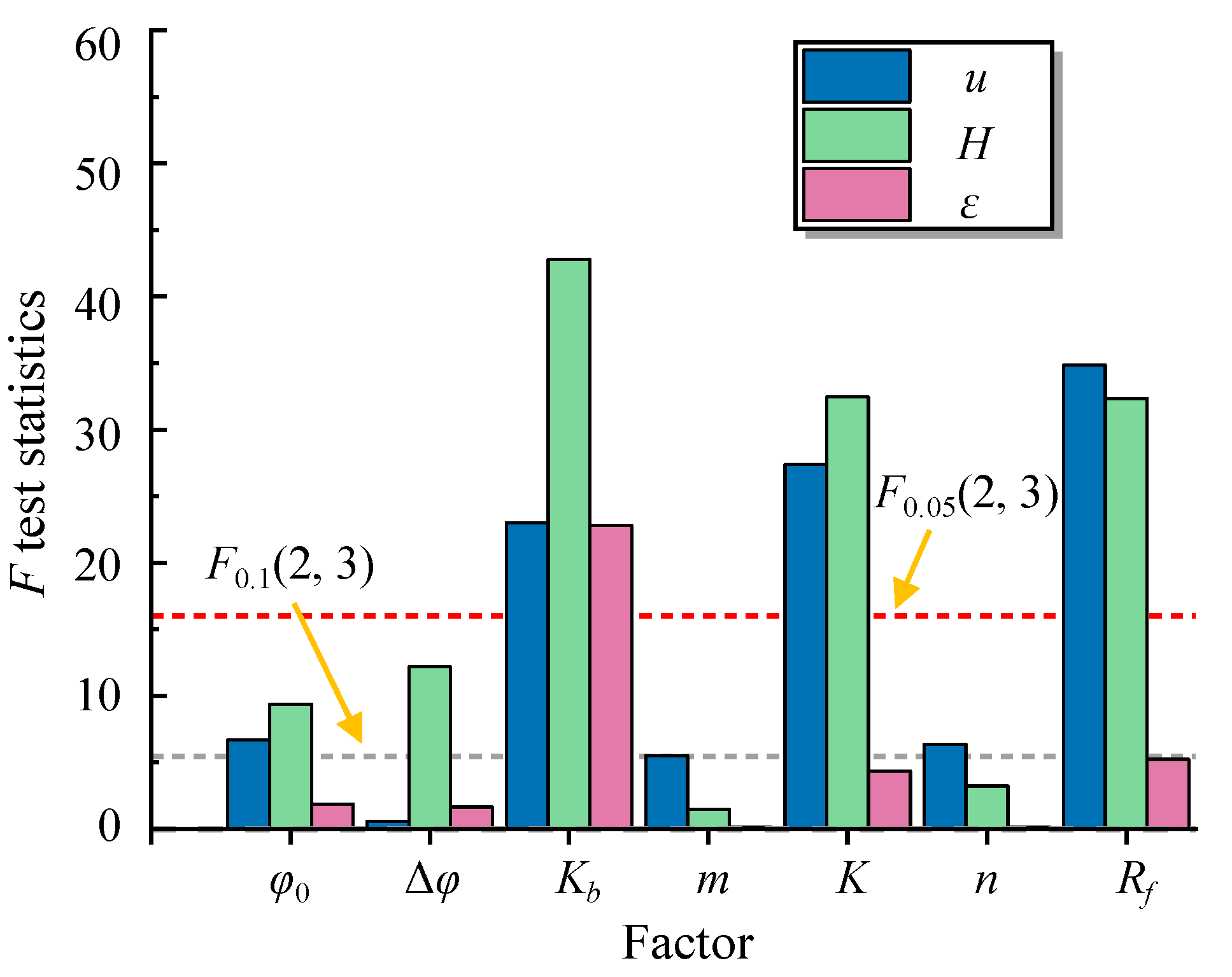
2. For the maximum vertical displacement of dam u, the sensitivity degree of the Duncan–Chang E-B model of the main rockfill zone parameters from high to low was Rf > φ0 > K > Kb > n > Δφ > m, the sensitivity degree of Rf was the highest; the sensitivity degree of the Duncan–Chang E-B model of the secondary rockfill zone parameters from high to low was Kb > K > Rf > φ0 > Δφ > m > n, the sensitivity degrees of Kb and K were high; the sensitivity degree of the Duncan–Chang E-B model of the reservoir bottom backfill zone parameters from high to low was Rf > K > Kb > n > φ0 > m > Δφ, the sensitivity degrees of Rf, K and Kb were highly significant, and the sensitivities were high.
3. For the maximum horizontal displacement of dam H, the sensitivity degree of the Duncan–Chang E-B model of the main rockfill zone parameters from high to low was Kb > Rf > K > φ0 > n > m > Δφ, and the sensitivities of Kb, Rf, K, and φ0 were highly significant, and the sensitivities were high; the sensitivity of the Duncan–Chang E-B model of the secondary rockfill zone parameters from high to low was Kb > Rf > K > φ0 > Δφ > m > n, the sensitivity of Kb was the highest; the sensitivity of the Duncan–Chang E-B model of the reservoir bottom backfill zone parameters from high to low was Kb > Rf > K > Δφ > φ0 > n > m, the sensitivities of Kb, K and Rf were high.
4. For the tensile strain of asphalt concrete ε, the sensitivity of the Duncan–Chang E-B model of main rockfill zone parameters from high to low was Kb > Rf > φ0 > K > n > m > Δφ, and the sensitivity of Kb was highly significant, and the sensitivity was high; the sensitivity of the Duncan–Chang E-B model of secondary rockfill zone parameters from high to low was Kb > K > φ0 > m > Δφ > n > Rf, e the sensitivity of Kb was the highest; the sensitivity of the Duncan–Chang E-B model of the reservoir bottom backfill zone parameters from high to low was Kb > Rf > K > φ0 > Δφ > n > m, the sensitivity of Kb was the highest.
5. The results of the range analysis were consistent with that of the variance analysis, which reflected the reliability of the sensitivity analysis in this study. Therefore, Kb, Rf, and K should be focused when analyzing PSPS’s ACFRD deformation with the Duncan–Chang E-B model, for which values were required to be accurate. For other parameters with low sensitivity, the engineering analogy method could be adopted to obtain the values. In this way, even if the measured data were missed, the calculation accuracy and efficiency could both be ensured. Furthermore, these sensitivity parameters should also be strictly controlled during the design and construction of ACFRD.
It should be noted that the mechanical properties of asphalt concrete are greatly affected by temperature changes. Therefore, for PSPS’s ACFRD deformation analysis in extremely cold or hot environments, the effect of temperature needs to be considered during modeling.

Author Contributions

Conceptualization, B.M., W.Z. and D.Z.; methodology, W.Z. and Z.S.; validation, B.M., W.Z. and D.Z.; formal analysis, W.Z.; resources, Z.S. and D.Z.; data curation, B.M., W.Z., H.Y. and R.W.; writing—original draft preparation, B.M., W.Z. and D.Z.; visualization, B.M. and W.Z., supervision, W.Z. and Z.S., project administration, Z.S., funding acquisition, W.Z. and Z.S. All authors have read and agreed to the published version of the manuscript.

Funding

This work was supported by the Project of National Natural Science Foundation of China (52179130, U1765205), the National Key R&D Program of China (2019YFC1510802), the Fundamental Research Funds for the Central Universities (B210203065), the Postgraduate Research & Practice Innovation Program of Jiangsu Province (KYCX21_0510), the Natural Science Foundation of Jiangsu Province (BK20201312), and the Priority Academic Program Development of Jiangsu Higher Education Institutions (Water Conservancy Project) (YS11001).

Data Availability Statement

Not applicable.

Acknowledgments

The authors are grateful to the reviewers and editors for their helpful and constructive comments, which significantly improved our manuscript.

Conflicts of Interest

The authors declare no conflict of interest.

References

  1. Luo, X.; Wang, J.; Dooner, M.; Clarke, J. Overview of current development in electrical energy storage technologies and the application potential in power system operation. Appl. Energy 2015, 137, 511–536. [Google Scholar] [CrossRef]
  2. Kong, Y.G.; Kong, Z.G.; Liu, Z.Q.; Wei, C.M.; Zhang, J.F.; An, G.C. Pumped-storage power stations in China: The past, the present, and the future. Renew. Sustain. Energy Rev. 2017, 71, 720–731. [Google Scholar] [CrossRef]
  3. Karimi, A.; Heydari, S.L.; Kouchakmohseni, F.; Naghiloo, M. Scheduling and value of pumped storage hydropower plant in Iran power grid based on fuel-saving in thermal units. J. Energy Storage 2019, 24, 100753. [Google Scholar] [CrossRef]
  4. Ma, K.; Feng, B.; Zhuang, D.Y.; Guo, X.F.; Gao, Q. Distance effects of the fault on the surrounding rock mass stability of the main powerhouse at the Huanggou pumped-storage power station. Tunn. Undergr. Space Technol. 2020, 106, 103568. [Google Scholar] [CrossRef]
  5. Luan, F.K.; Yuan, B.; Cao, C.; Yang, J.; Xu, Z.C. Future development and features of pumped storage stations in China. In Proceedings of the 1st International Conference on Environment Prevention and Pollution Control Technology (EPPCT), Tokyo, Japan, 9–11 November 2018. [Google Scholar]
  6. Gao, J.; Dang, F.N.; Ma, Z.Y. Investigation for the key technologies of ultra-high asphalt concrete core rockfill dams. Soils Found. 2019, 59, 1740–1757. [Google Scholar] [CrossRef]
  7. Xu, H.N.; Xing, C.; Zhang, H.Y.; Li, H.Z.; Tan, Y.Q. Moisture seepage in asphalt mixture using X-ray imaging technology. Int. J. Heat Mass Transf. 2019, 131, 375–384. [Google Scholar] [CrossRef]
  8. Lee, S.-H.; Eum, K.-Y.; Le, T.H.M.; Park, D.-W. Evaluation on mechanical behavior of asphalt concrete trackbed with slab panel using full-scale static and dynamic load test. Constr. Build. Mater. 2021, 276, 122207. [Google Scholar] [CrossRef]
  9. Zou, C.G.; Hua, Z.; Mo, L.T.; Qi, C.; Liu, Z.X.; Xie, Y.J.; Yu, H.; Ke, J.T. Evaluation on the performance of hydraulic bitumen binders under high and low temperatures for pumped storage power station projects. Materials 2022, 15, 1890. [Google Scholar] [CrossRef]
  10. Zhang, G.; Zhang, J.M. Numerical modeling of soil-structure interface of a concrete-faced rockfill dam. Comput. Geotech. 2009, 36, 762–772. [Google Scholar] [CrossRef]
  11. Yang, C.; Shen, Z.Z.; Tan, J.C.; Li, G.H. Analytical method for estimating leakage of reservoir basins for pumped storage power stations. Bull. Eng. Geol. Environ. 2021, 80, 5145–5158. [Google Scholar] [CrossRef]
  12. Jappelli, R.; Bertacchi, P.; Callari, C.; Cazzuffi, D.; Maio, S.D.; Sarti, L.; Sembenelli, P. Embankment Dams with Bituminous Concrete Upstream Facing: Review and Recommendations, International Commission on Large Dams (ICOLD) Bulletin n. 114. 1999. Available online: https://www.researchgate.net/publication/347228515_Embankment_Dams_with_Bituminous_Concrete_Upstream_Facing_Review_and_Recommendations_International_Commission_on_Large_Dams_ICOLD_Bulletin_n_114 (accessed on 30 July 2022).
  13. Špano, M.; Říha, J.; Španová, A.; Šedo, O.; Rittich, B. Bacterial diversity in the asphalt concrete lining of the upper water reservoir of a pumped-storage scheme. Water 2020, 12, 3045. [Google Scholar] [CrossRef]
  14. Wang, Z.; Hao, J.; Sun, Z.; Ma, B.; Xia, S.; Li, X. Blistering mechanism analysis of hydraulic asphalt concrete facing. Appl. Sci. 2019, 9, 2903. [Google Scholar] [CrossRef]
  15. Djemili, L.; Chiblak, M.M. Study of the temperature distribution in the bituminous concrete facing used in fill dams in the region of west Algeria. J. Eng. Appl. Sci. 2007, 8, 576–579. [Google Scholar] [CrossRef]
  16. Adam, K.; Říha, J.; Spano, M. Investigation on the temperature of the asphalt-concrete facing of embankment dams. Int. J. Pavement Res. Technol. 2016, 9, 73–81. [Google Scholar] [CrossRef]
  17. Leon, L.P.; Gay, D.; Simpson, N.; Edwin, S. Stress-strain and failure modes of asphalt concrete in compression due to geometrical changes. In Proceedings of the 16th LACCEI International Multi-Conference for Engineering, Education, and Technology, Innovation in Education and Inclusion, Lima, Peru, 18–20 July 2018. [Google Scholar]
  18. Li, Y.L.; Tang, W.; Wen, L.F.; Wu, H.B. Dam seismic deformation evaluation method of asphalt concrete core rockfill dam and its reliability analysis. J. Hydraul. Eng. 2020, 51, 580–588. (In Chinese) [Google Scholar] [CrossRef]
  19. Yang, K.; He, Z.; Li, D.; Xu, H.; Kong, L. Experimental Study on Basalt Fiber Crack Resistance of Asphalt Concrete Based on Acoustic Emission. Materials 2021, 14, 4096. [Google Scholar] [CrossRef]
  20. Hao, J.; Cao, P.; Liu, Z.; Wang, Z.; Xia, S. Developing of a SBS polymer modified bitumen to avoid low temperature cracks in the asphalt facing of a reservoir in a harsh climate region. Constr. Build. Mater. 2017, 150, 105–113. [Google Scholar] [CrossRef]
  21. Chen, Y.; Zhao, W.; Jia, P.-J.; Han, J.-Y. Proportion Analysis of Ground Settlement Caused by Excavation and Dewatering of A Deep Excavation in Sand Area. Indian Geotech. J. 2018, 48, 103–113. [Google Scholar] [CrossRef]
  22. Chen, Y.; Zhao, W.; Han, J.; Jia, P. A CEL study of bearing capacity and failure mechanism of strip footing resting on c-φ soils. Comput. Geotech. 2019, 111, 126–136. [Google Scholar] [CrossRef]
  23. Xu, Q.; Solaimanian, M. Modelling linear viscoelastic properties of asphalt concrete by the Huet–Sayegh model. Int. J. Pavement Eng. 2009, 10, 401–422. [Google Scholar] [CrossRef]
  24. Dong, W.; Hu, L.; Yu, Y.Z.; Lv, H. Comparison between Duncan and Chang’s EB Model and the Generalized Plasticity Model in the Analysis of a High Earth-Rockfill Dam. J. Appl. Math. 2013, 2013, 709430. [Google Scholar] [CrossRef]
  25. Khoshghalb, A.; Khalili, N. A meshfree method for fully coupled analysis of flow and deformation in unsaturated porous media. Int. J. Numer. Anal. Methods Géoméch. 2013, 37, 716–743. [Google Scholar] [CrossRef]
  26. Qian, J.; You, Z.; Huang, M.; Gu, X. A micromechanics-based model for estimating localized failure with effects of fabric anisotropy. Comput. Geotech. 2013, 50, 90–100. [Google Scholar] [CrossRef]
  27. Shahbodagh, B.; Habte, M.; Khoshghalb, A.; Khalili, N. A bounding surface elasto-viscoplastic constitutive model for non-isothermal cyclic analysis of asphaltic materials. Int. J. Numer. Anal. Methods Géoméch. 2017, 41, 721–739. [Google Scholar] [CrossRef]
  28. Huang, M.; Chen, Z.; Lu, X. Bifurcation prediction of shear banding in sand with non-coaxial critical state model considering inherent anisotropy. Soils Found. 2018, 58, 641–653. [Google Scholar] [CrossRef]
  29. Ghaffaripour, O.; Esgandani, G.A.; Khoshghalb, A.; Shahbodaghkhan, B. Fully coupled elastoplastic hydro-mechanical analysis of unsaturated porous media using a meshfree method. Int. J. Numer. Anal. Methods Géoméch. 2019, 43, 1919–1955. [Google Scholar] [CrossRef]
  30. Zhao, G.-F.; Lian, J.; Russell, A.; Khalili, N. Implementation of a modified Drucker–Prager model in the lattice spring model for plasticity and fracture. Comput. Geotech. 2019, 107, 97–109. [Google Scholar] [CrossRef]
  31. Wu, M.; Gao, X.; Lin, H. Simulation analysis of the deformation behavior of nanoindentation based on elasto–plastic constitutive model. Polym. Bull. 2022. Available online: https://www.researchgate.net/publication/361082891_Simulation_analysis_of_the_deformation_behavior_of_nanoindentation_based_on_elasto-plastic_constitutive_model (accessed on 30 July 2022). [CrossRef]
  32. Sternik, K. Elasto-plastic Constitutive Model for Overconsolidated Clays. Int. J. Civ. Eng. 2017, 15, 431–440. [Google Scholar] [CrossRef]
  33. Jia, P.; Khoshghalb, A.; Chen, C.; Zhao, W.; Dong, M.; Esgandani, G.A. Modified Duncan-Chang Constitutive Model for Modeling Supported Excavations in Granular Soils. Int. J. Géoméch. 2020, 20, 04020211. [Google Scholar] [CrossRef]
  34. Guo, P.; Li, W.-C. Development and implementation of Duncan-Chang constitutive model in GeoStudio2007. Procedia Eng. 2012, 31, 395–402. [Google Scholar] [CrossRef]
  35. Wang, Z.; Liu, X.; Yang, X.; Fu, Y. An improved Duncan-Chang constitutive model for sandstone subjected to drying-wetting cycles and secondary development of the model in FLAC3D. Arab. J. Sci. Eng. 2017, 42, 1265–1282. [Google Scholar] [CrossRef]
  36. Ni, P.; Mei, G.; Zhao, Y.; Chen, H. Plane strain evaluation of stress paths for supported excavations under lateral loading and unloading. Soils Found. 2018, 58, 146–159. [Google Scholar] [CrossRef]
  37. Zhang, X.Z.; Wang, R.H.; Jia, B. The Experiment Study on Parameters of Duncan-Chang Model for Silt Based on Different Water Content. Appl. Mech. Mater. 2014, 665, 213–216. [Google Scholar] [CrossRef]
  38. Zhang, B. Analysis on Parameters in Duncan-Chang Constitutive Model. Adv. Mater. Res. 2011, 368–373, 2900–2903. [Google Scholar] [CrossRef]
  39. Jia, Y.; Xu, B.; Chi, S.; Xiang, B.; Xiao, D.; Zhou, Y. Joint back analysis of the creep deformation and wetting deformation parameters of soil used in the Guanyinyan composite dam. Comput. Geotech. 2018, 96, 167–177. [Google Scholar] [CrossRef]
  40. Jia, Y.; Chi, S. Back-analysis of soil parameters of the Malutang II concrete face rockfill dam using parallel mutation particle swarm optimization. Comput. Geotech. 2015, 65, 87–96. [Google Scholar] [CrossRef]
  41. Hu, S.; Chen, Y.; Liu, W.; Zhou, S.; Hu, R. Effect of seepage control on stability of a tailings dam during its staged construction with a stepwise-coupled hydro-mechanical model. Int. J. Min. Reclam. Environ. 2015, 29, 125–140. [Google Scholar] [CrossRef]
  42. Zhang, W.; Shen, Z.; Ren, J.; Bian, J.; Xu, L.; Chen, G. Multifield Coupling Numerical Simulation of the Seepage and Stability of Embankment Dams on Deep Overburden Layers. Arab. J. Sci. Eng. 2022, 47, 7293–7308. [Google Scholar] [CrossRef]
  43. Li, Y.; She, L.; Wen, L.; Zhang, Q. Sensitivity analysis of drilling parameters in rock rotary drilling process based on orthogonal test method. Eng. Geol. 2020, 270, 105576. [Google Scholar] [CrossRef]
  44. Zhang, W.; Shen, Z.; Ren, J.; Gan, L.; Xu, L.; Sun, Y. Phase-field simulation of crack propagation in quasi-brittle materials: COMSOL implementation and parameter sensitivity analysis. Model. Simul. Mater. Sci. Eng. 2021, 229, 055020. [Google Scholar] [CrossRef]
  45. Duncan, J.M.; Chang, C.-Y. Nonlinear Analysis of Stress and Strain in Soils. J. Soil Mech. Found. Div. 1970, 96, 1629–1653. [Google Scholar] [CrossRef]
  46. Coulomb, C.A. Essai sur une application des règles de maximis & minimis à quelques problèmes de statique, relatifs à l’architecture. Acad. R. Des. Sci. 1973, 7, 343–382. [Google Scholar]
  47. Mohr, O. Abhandlungen aus dem Gebiete der Technischen Mechanik, 2nd ed.; Ernst: Berlin, Germany, 1914. [Google Scholar]
  48. Gan, L.; Shen, Z.-Z.; Xu, L.-Q. Long-Term Deformation Analysis of the Jiudianxia Concrete-Faced Rockfill Dam. Arab. J. Sci. Eng. 2014, 39, 1589–1598. [Google Scholar] [CrossRef]
  49. Gan, L.; Shen, X.; Zhang, H. New deformation back analysis method for the creep model parameters using finite element nonlinear method. Clust. Comput. 2017, 20, 3225–3236. [Google Scholar] [CrossRef]
  50. Ren, J.; Zhang, W.; Yang, J.; Shen, Z.; Zhao, J.; Zhou, Y.; Wang, Z. A comparison of numerical and Lu modeling of water flow and heat transport with laboratory experiments. Environ. Earth Sci. 2019, 78, 267. [Google Scholar] [CrossRef]
  51. Fang, C.; Liu, Z. Stress-strain analysis of Aikou rockfill dam with asphalt-concrete core. J. Rock Mech. Geotech. Eng. 2011, 3, 186–192. [Google Scholar] [CrossRef]
  52. Alamnie, M.M.; Taddesse, E.; Hoff, I. Advances in Permanent Deformation Modeling of Asphalt Concrete—A Review. Materials 2022, 15, 3480. [Google Scholar] [CrossRef]
  53. Wang, W.B.; Sun, Z.T.; Wu, L.Y. Study on stress-strain relationship of asphalt concrete. J. Hydraul. Eng. 1996, 5, 1–8+28. (In Chinese) [Google Scholar] [CrossRef]
Figure 1. (a) Geographical location map; (b) layout of the reservoir site.
Water 14 02634 g001
Figure 2. Typical cross-section of the main dam along the river (unit: m).
Water 14 02634 g002
Figure 3. Three-dimensional finite element mesh of the calculation zone: (a) reservoir basin; (b) reservoir bottom backfill area; (c) asphalt concrete face; (d) dam rock area.
Water 14 02634 g003
Figure 4. Step loading and water storage process of the model.
Water 14 02634 g004
Figure 5. Distribution of horizontal displacement along the river (unit: mm): (a) after completion; (b) after impoundment.
Water 14 02634 g005
Figure 6. Distribution of vertical displacement (unit: mm): (a) after completion; (b) after impoundment.
Water 14 02634 g006
Figure 7. Distribution of tensile strain of asphalt concrete face after impoundment (unit: %).
Water 14 02634 g007
Figure 8. Sensitivity of each index for the main rockfill zone.
Water 14 02634 g008
Figure 9. Sensitivity of each test index for the secondary rockfill zone.
Water 14 02634 g009
Figure 10. Sensitivity of each test index for the reservoir bottom backfill zone.
Water 14 02634 g010
Figure 11. ANOVA results of each parameter in the main rockfill zone to different indexes.
Water 14 02634 g011
Figure 12. ANOVA results of each parameter in secondary rockfill zone to different indexes.
Water 14 02634 g012
Figure 13. ANOVA results of each parameter in reservoir bottom backfill zone to different indexes.
Water 14 02634 g013
Table 1. L18 (2 × 37) orthogonal table.
Test NumberColumn Number
12345678
111111111
211222222
311333333
412112233
512223311
612331122
713121323
813232131
913313212
1021133221
1121211332
1221322113
1322123132
1422231213
1522312321
1623132312
1723213123
1823321231
Table 2. Calculation parameters for Duncan–Chang E-B model materials.
Materialρ/(g·cm−3)φ0φKbmKnRf
Cushion material2.242.2411.1498.20.231241.20.300.74
Transition material2.2156.412.1526.70.031324.30.250.72
Main rockfill2.1855.613.0294.90.03969.00.250.71
Secondary rockfill2.1755.013.1237.20.12813.40.230.70
Rockfill behind the dam2.1653.412.4162.80.15747.20.230.70
Reservoir bottom backfill2.1653.412.4162.80.15747.20.230.70
Asphalt concrete2.4030.04.201292.10.40825.90.550.47
Table 3. Calculation parameters for linear elastic model materials.
MaterialVolumetric Weight γ/kN∙m−3Elastic Modulus E/GPaPoisson’s Ratio ν
Concrete wave wall24.028.00.167
Strongly weathered bedrock26.620.00.250
Weakly weathered bedrock28.450.00.250
Table 4. Factor levels for orthogonal test.
ZoneFactor Levelφ0 (°)Δφ (°)KbmKnRf
Main rockfill144.4810.40235.920.024775.200.2000.568
255.6013.00294.900.030969.000.2500.710
366.7215.60353.880.0361162.800.3000.852
Secondary rockfill144.0010.48189.760.096650.720.1840.560
255.0013.10237.200.120813.400.2300.700
366.0015.72284.640.144976.080.2760.840
Reservoir bottom backfill142.729.920130.240.120597.760.1840.560
253.4012.40162.800.150747.200.2300.700
364.0814.88195.360.180896.640.2760.840
Table 5. Orthogonal test scheme and calculation results of main rockfill zone.
SchemeEmpty Columnφ0 (°)Δφ (°)KbmKnRfu/cmH/cmε/%
1144.4810.4235.920.024775.20.200.5685.751−54.952−0.348
2144.4813.0294.900.030969.00.250.7106.849−49.394−0.408
3144.4815.6353.880.0361162.80.300.8528.080−45.835−0.464
4155.6010.4235.920.030969.00.300.8526.288−55.851−0.362
5155.6013.0294.900.0361162.80.200.5684.298−41.551−0.371
6155.6015.6353.880.024775.20.250.7108.404−45.892−0.451
7166.7210.4294.900.0241162.80.250.8526.064−47.026−0.400
8166.7213.0353.880.030775.20.300.5683.565−39.789−0.415
9166.7215.6235.920.036969.00.200.7105.257−52.364−0.349
10244.4810.4353.880.036969.00.250.5685.958−40.957−0.471
11244.4813.0235.920.0241162.80.300.7105.285−51.644−0.351
12244.4815.6294.900.030775.20.200.85210.698−57.170−0.456
13255.6010.4294.900.036775.20.300.7106.982−48.559−0.404
14255.6013.0353.880.024969.00.200.8528.621−46.753−0.467
15255.6015.6235.920.0301162.80.250.5684.035−43.388−0.347
16266.7210.4353.880.0301162.80.200.7105.789−40.488−0.418
17266.7213.0235.920.036775.20.250.8527.472−58.165−0.379
18266.7215.6294.900.024969.00.300.5684.334−41.853−0.369
Table 6. Orthogonal test scheme and calculation results of secondary rockfill zone.
SchemeEmpty Columnφ0 (°)Δφ (°)KbmKnRfu/cmH/cmε/%
114410.48189.760.096650.720.1840.567.253−49.164−0.402
214413.10237.200.120813.400.2300.706.120−47.333−0.395
314415.72284.640.144976.080.2760.845.077−45.942−0.389
415510.48189.760.120813.400.2760.846.934−49.052−0.401
515513.10237.200.144976.080.1840.566.601−46.128−0.394
615515.72284.640.096650.720.2300.704.150−46.209−0.386
716610.48237.200.096976.080.2300.846.018−47.180−0.394
816613.10284.640.120650.720.2760.564.408−45.656−0.385
916615.72189.760.144813.400.1840.707.065−48.570−0.400
1024410.48284.640.144813.400.2300.565.314−45.503−0.388
1124413.10189.760.096976.080.2760.707.555−48.173−0.401
1224415.72237.200.120650.720.1840.844.715−47.923−0.392
1325510.48237.200.144650.720.2760.705.208−47.175−0.391
1425513.10284.640.096813.400.1840.844.462−46.276−0.388
1525515.72189.760.120976.080.2300.567.091−46.712−0.396
1626610.48284.640.120976.080.1840.705.295−45.533−0.388
1726613.10189.760.144650.720.230.845.874−49.213−0.397
1826615.72237.20.096813.40.2760.566.453−46.663−0.394
Table 7. Orthogonal test scheme and calculation results of reservoir bottom backfill zone.
SchemeEmpty Columnφ0 (°)Δφ (°)KbmKnRfu/cmH/cmε/%
1142.729.92130.240.12597.760.1840.565.916−47.179−0.466
2142.7212.40162.800.15747.200.2300.706.069−47.133−0.394
3142.7214.88195.360.18896.640.2760.846.226−47.075−0.330
4153.409.92130.240.15747.200.2760.846.131−47.146−0.502
5153.4012.40162.800.18896.640.1840.565.865−47.116−0.331
6153.4014.88195.360.12597.760.2300.706.270−47.027−0.335
7164.089.92162.800.12896.640.2300.846.183−47.116−0.413
8164.0812.40195.360.15597.760.2760.566.147−47.067−0.328
9164.0814.88130.240.18747.200.1840.706.014−47.159−0.472
10242.729.92195.360.18747.200.2300.566.030−47.126−0.323
11242.7212.40130.240.12896.640.2760.705.845−47.178−0.411
12242.7214.88162.800.15597.760.1840.846.354−47.040−0.405
13253.409.92162.800.18597.760.2760.706.192−47.099−0.389
14253.4012.40195.360.12747.200.1840.846.316−47.044−0.335
15253.4014.88130.240.15896.640.2300.565.840−47.150−0.329
16264.089.92195.360.15896.640.1840.706.110−47.101−0.335
17264.0812.40130.240.18597.760.2300.846.312−47.091−0.497
18264.0814.88162.800.12747.200.2760.565.918−47.154−0.374
Table 8. Range analysis results of influencing factors of each test index for the main rockfill zone.
Test IndexFactorφ0 (°)Δφ (°)KbmKnRf
uK1j0.7852−0.1797−0.63700.09150.82700.4173−1.6615
K2j0.1197−0.30330.2192−0.1143−0.10050.14530.1093
K3j−0.90480.48300.41780.0228−0.7265−0.56271.5522
Rj1.69000.78631.05480.20581.55350.98003.2137
HK1j−2.1236−0.1038−4.8589−0.1516−2.8861−1.01134.1201
K2j0.8694−0.01430.27620.18840.00640.3981−0.1884
K3j1.25420.11814.5827−0.03682.87970.6132−3.9316
Rj3.37780.22199.44160.34005.76581.62458.0517
εK1j0.1481−0.0124−0.4579−0.04210.0730−0.0021−0.1484
K2j−0.0148−0.0308−0.0190−0.00660.02600.0759−0.0476
K3j−0.13330.04320.45990.0487−0.0991−0.07380.1961
Rj0.28140.07400.91780.09080.17210.14970.3445
Table 9. Range analysis results of influencing factors on each test index for the secondary rockfill zone.
Test IndexFactorφ0 (°)Δφ (°)KbmKnRf
uK1j0.13940.13741.09570.1156−0.59830.03220.3204
K2j−0.1253−0.0296−0.0138−0.105780.1917−0.10510.0324
K3j−0.0141−0.1078−1.0819−0.00980.40660.0729−0.3529
Rj0.26470.24522.17760.22141.00490.17800.6733
HK1j−0.2060−0.1342−1.3471−0.1439−0.4231−0.13210.4959
K2j0.20820.00380.06660.0988−0.09920.1086−0.0319
K3j−0.00220.13041.28040.04510.52230.0234−0.4641
Rj0.41420.26462.62750.24270.94540.24070.9600
εK1j0.01220.00620.06190.0072−0.01210.0047−0.0029
K2j−0.0078−0.0013−0.0016−0.00540.0086−0.00610.0019
K3j−0.0044−0.0049−0.0603−0.00180.00360.00140.0011
Rj0.02000.01110.12220.01260.02070.01080.0048
Table 10. Range analysis results of influencing factors of each test index for the reservoir bottom backfill zone.
Test IndexFactorφ0 (°)Δφ (°)KbmKnRf
uK1j−0.0232−0.0029−0.0869−0.02190.1019−0.0007−0.1439
K2j0.0058−0.00420.00030.0119−0.01690.0208−0.0132
K3j0.01740.00710.08660.0010−0.0851−0.02010.1571
Rj0.04060.01130.17350.03380.18700.04090.3010
HK1j−0.0232−0.0029−0.0869−0.02190.1019−0.0007−0.1439
K2j0.0058−0.00420.00030.0119−0.01690.0208−0.0132
K3j0.01740.00710.08660.0010−0.0851−0.02010.1571
Rj0.04060.01130.17350.03380.18700.04090.3010
εK1j0.01090.17340.58920.01890.16220.0342−0.2856
K2j−0.1709−0.0439−0.0279−0.05030.1282−0.05280.0201
K3j0.1601−0.1294−0.56130.0314−0.29040.01860.2656
Rj0.33100.30281.15050.08170.45260.08700.5512
Table 11. ANOVA results of influencing factors of each test index for the main rockfill zone.
Test IndexSource of VarianceSum of Squares of Deviations SjDegree of Freedom fjStatistics FjSignificance
uφ08.697228.3728Generally significant
Δφ2.145522.0655Not significant
Kb3.770323.6297Not significant
m0.1317920.1269Not significant
K7.331027.0575Generally significant
n3.071322.9567Not significant
Rf31.091229.931Highly significant
Random error1.558123
Hφ041.032216.032Highly significant
Δφ0.149520.0584Not significant
Kb268.122104.76Highly significant
m0.359020.1403Not significant
K99.735238.969Highly significant
n9.343023.6501Not significant
Rf194.81276.117Highly significant
Random error3.83903
εφ00.239424.8606Not significant
Δφ0.017820.3618Not significant
Kb2.5273251.310Highly significant
m0.025120.5105Not significant
K0.095021.9294Not significant
n0.067221.3651Not significant
Rf0.376427.6426Generally significant
Random error0.07393
Table 12. ANOVA results of influencing factors of each test index for the secondary rockfill zone.
Test IndexSource of VarianceSum of Squares of Deviations SjDegree of Freedom fjStatistics FjSignificance
uφ00.211921.1768Not significant
Δφ0.188221.0450Not significant
Kb14.228279.003Highly significant
m0.147820.8208Not significant
K3.3599218.656Highly significant
n0.104420.5797Not significant
Rf1.369727.6051Generally significant
Random error0.27013
Hφ00.515122.0988Not significant
Δφ0.210320.8568Not significant
Kb20.751284.557Highly significant
m0.1950020.7945Not significant
K2.7696211.286Generally significant
n0.178720.7282Not significant
Rf2.7740211.303Generally significant
Random error0.36813
εφ00.001422.3810Not significant
Δφ0.000420.6719Not significant
Kb0.0448277.415Highly significant
m0.000520.8810Not significant
K0.001422.4109Not significant
n0.000420.6384Not significant
Rf0.000120.1384Not significant
Random error0.00093
Table 13. ANOVA results of influencing factors of each test index for the reservoir bottom backfill zone.
Test IndexSource of VarianceSum of Squares of Deviations SjDegree of Freedom fjStatistics FjSignificance
uφ00.005326.7039Generally significant
Δφ0.000520.5866Not significant
Kb0.09032115.06Highly significant
m0.004325.5092Generally significant
K0.10752136.93Highly significant
n0.005026.3790Generally significant
Rf0.27342348.30Highly significant
Random error0.00123
Hφ00.002029.3796Generally significant
Δφ0.0025212.191Generally significant
Kb0.0179285.571Highly significant
m0.000321.4848Not significant
K0.0068232.442Highly significant
n0.000723.2408Not significant
Rf0.0068232.337Highly significant
Random error0.00033
εφ00.329821.8892Not significant
Δφ0.292521.6758Not significant
Kb3.9780222.791Highly significant
m0.023220.1330Not significant
K0.762724.3697Not significant
n0.025820.1478Not significant
Rf0.915025.2421Not significant
Random error0.26183
Table 14. Sensitivity results of range analysis and ANOVA.
ZoneAnalysis MethoduHε
Main rockfill zoneRange analysis methodRf > φ0 > K > Kb > n > Δφ > mKb > Rf > K > φ0 > n > m > ΔφKb > Rf > φ0 > K > n > m > Δφ
ANVOA methodRf > φ0 > K > Kb > n > Δφ > mKb > Rf > K > φ0 > n > m > ΔφKb > Rf > φ0 > K > n > m > Δφ
Secondary rockfill zoneRange analysis methodKb > K > Rf > φ0 > Δφ > m > nKb > Rf > K > φ0 > Δφ > m > nKb > K > φ0 > m > Δφ > n > Rf
ANVOA methodKb > K > Rf > φ0 > Δφ > m > nKb > Rf > K > φ0 > Δφ > m > nKb > K > φ0 > m > Δφ > n > Rf
Reservoir bottom backfill zoneRange analysis methodRf > K > Kb > n > φ0 > m > ΔφKb > Rf > K > Δφ > φ0 > n > mKb > Rf > K > φ0 > Δφ > n > m
ANVOA methodRf > K > Kb > n > φ0 > m > ΔφKb > Rf > K > Δφ > φ0 > n > mKb > Rf > K > φ0 > Δφ > n > m
Publisher’s Note: MDPI stays neutral with regard to jurisdictional claims in published maps and institutional affiliations.

