

Improved Monthly and Seasonal Multi-Model Ensemble Precipitation Forecasts in Southwest Asia Using Machine Learning Algorithms

1
Atmospheric Science and Meteorological Research Center (ASMERC), Climate Research Institute (CRI), Mashhad, Iran
2
Climate Service Center Germany (GERICS), Helmholtz-Zentrum Hereon, Fischertwiete 1, 20095 Hamburg, Germany
*
Authors to whom correspondence should be addressed.
Water 2022, 14(17), 2632; https://doi.org/10.3390/w14172632
Submission received: 7 July 2022
/
Revised: 18 August 2022
/
Accepted: 19 August 2022
/
Published: 26 August 2022
(This article belongs to the Special Issue Artificial Intelligence Techniques in Hydrology and Water Resources Management)
Abstract
:Southwest Asia has different climate types including arid, semiarid, Mediterranean, and temperate regions. Due to the complex interactions among components of the Earth system, forecasting precipitation is a difficult task in such large regions. The aim of this paper is to propose a learning approach, based on artificial neural network (ANN) and random forest (RF) algorithms for post-processing the output of forecasting models, in order to provide a multi-model ensemble forecasting of monthly precipitation in southwest Asia. For this purpose, four forecasting models, including GEM-NEMO, NASA-GEOSS2S, CanCM4i, and COLA-RSMAS-CCSM4, included in the North American multi-model ensemble (NMME) project, are considered for the ensemble algorithms. Since each model has nine different lead times, a total of 108 different ANN and RF models are trained for each month of the year. To train the proposed ANN an RF models, the ERA5 reanalysis dataset is employed. To compare the performance of the proposed algorithms, four performance evaluation criteria are calculated for each model. The results indicate that the performance of the ANN and RF post-processing is better than that of the individual NMME models. Moreover, RF outperformed ANN for all lead times and months of the year.
1. Introduction
The accurate forecasting of precipitation has been an important topic from both theoretical points of view and practical applications. Many researchers around the world are working to improve the accuracy of monthly and seasonal weather forecasts. Such forecasts are essential for various water resource planning practices, as well as related actions for agricultural planning and securing food supplies in many regions of the world. With increasing populations that rely on such water resources and the increasing impact of climatic variations and climate change, requirements for the accuracy of such forecasts are also increasing. Different computational methods are used for improving forecasts that are generally divided into two categories: dynamical and statistical methods for post-processing the outputs of General circulation models (GCMs). The performance of these techniques can vary for different geographical areas with different topographies and climate types.
Among the computational methods for post-processing the output of forecasts, the use of machine learning (ML) techniques is very widespread. ML theory employs several types of tools such as fuzzy systems (e.g., [1]), artificial neural networks, decision trees, and so on. The widespread use of these techniques can be attributed to the ability of these methods to model Big Data and their flexibility in calculations, as well as their increased abilities to use such techniques with available modern computational resources. Examples in hydrology include flood forecasting applications (see e.g., [2]) and climate modelling applications for sub-grid processes ([3]).
In seasonal weather forecasting, [4] employed artificial neural networks (ANNs) for the monthly forecasting of precipitation over Iran, and used the outputs of the North American multi-model ensemble (NMME) project. They also used other machine learning techniques including ANN, support vector regression, decision tree, and random forests for the monthly forecast of precipitation [5]. Ref. [6] used the non-linear autoregressive neural network (NARNN), non-linear input–output (NIO), and NARNN with exogenous input (NARNNX), for annual precipitation forecasting over 27 precipitation stations located in Gilan, Iran. Their results showed that the accuracy of the NARNNX was better than that of the NARNN and NIO. Ref. [7] proposed a model for the monthly forecasting of precipitation for East Azarbaijan in Iran, over a ten-year period using the multilayer perceptron neural network (MLP) and support vector regression (SVR) models. They employed the flow regime optimization algorithm (FRA) for training step in multilayer neural network and support vector machine. Ref. [8] constructed an artificial neural network model for generating probabilistic subseasonal precipitation forecasts over California. They used an artificial neural network (ANN) to establish relationships between the 7-day accumulated precipitation of numerical weather prediction (NWP) ensemble forecast. Ref. [9] tried to use the random-forest-based machine learning algorithm for nowcasting convective rain in Kolkata, India, with a ground-based radiometer. They found that their proposed model is very sensitive to the boundary layer instability, as indicated by the variable importance measure. Their study showed the suitability of a random forest algorithm for nowcasting the application and other forecasting problems. Ref. [10] used the ensemble precipitation forecasts of six numerical models from the THORPEX Interactive Grand Global Ensemble (TIGGE) database, associated with four basins in Iran for 2008–2018, which were extracted and bias-corrected by the quantile mapping (QM) and random forest (RF) methods. Their results demonstrated that most models had better skills in forecasting precipitation depth after bias correction using the RF method, compared to using the QM method and raw forecasts. Ref. [11] used random forests and regression tree for quantitative precipitation estimates with operational dual-polarization radar data. The use of neural networks and machine learning techniques is not limited to precipitation forecasting. For example, Ref. [12] used decision tree and neural networks for lightning prediction. Ref. [13] used a kernel least mean square algorithm for solving fuzzy differential equations and studied its application in earth’s energy balance model and climate. Ref. [14] studied the theoretical impact of changing albedo on precipitation and [15] found that fuzzy uncertainty for albedo creates more real results after solving the fuzzy energy balance equation. For some other applications of machine learning in climate modeling, see [16,17,18,19,20,21,22,23].
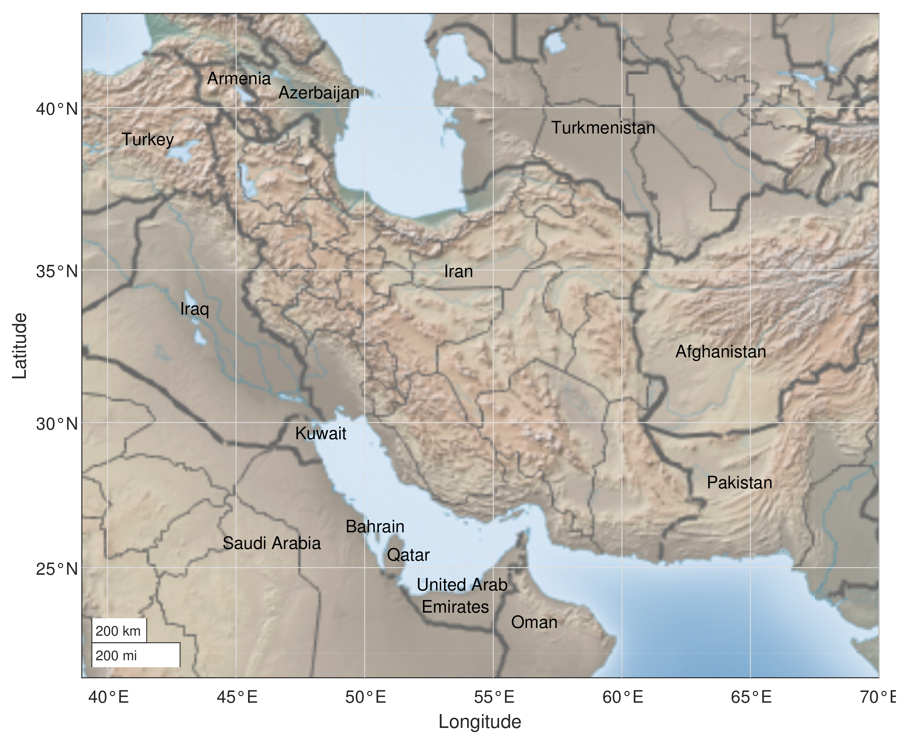
Southwest Asia contains many geographical features including water bodies of Caspian Sea, Persian Gulf, Oman Sea, Arabian Sea, and elongated mountains of Zagros and Alborz, as well as widespread deserts in Saudi Arabia, Iraq, and Iran (Lut and Dasht-e-Kavir). The region has different types of climates including arid, semiarid, Mediterranean, and temperate regions. Due to complex interactions among components of the earth and weather systems, the forecasting of precipitation is a difficult task in such large regions. Several researches have conducted monthly forecasts of precipitation in this region and countries therein. Ref. [24] studied the attributes of precipitation for the Middle East and southwest Asia during periods of enhanced or reduced tropical eastern Indian Ocean precipitation associated with opposing phases of the Madden–Julian oscillation (MJO). They used multiple estimates of both observed precipitation and MJO state during November–April 1981–2016 to provide a more robust assessment in this data-limited region. Ref. [25] assessed the sensitivity of southwest Asia precipitation during the November–April rainy season to four types of El Niño–Southern Oscillation (ENSO) events, El Niño and La Niña, using an ensemble of climate model simulations forced by 1979–2015 boundary conditions. Ref. [26] studied the potential predictability and skill of boreal winter (December to February: DJF) precipitation over central-southwest Asia by using six models of the North American multi-model ensemble project for the period 1983–2018. Ref. [27] explored the predictability of central-southwest Asia wintertime precipitation based on its time-lagged relationship with the preceding months’ (September–October) sea surface temperature (SST), using a canonical correlation analysis (CCA) approach. They showed that the regional potential predictability has a strong dependency on the ENSO phenomenon, and the strengthening (weakening) of this relationship yields forecasts with higher (lower) predictive skill. Based on the literature review, there are various studies in precipitation forecasting for the countries of the Southwest Asian region separately. However, there is no integrated approach based on machine learning methods as well as MME approaches that consider multiple countries simultaneously. Although extending the computations to a larger area increases the computational costs, it can better model large precipitation patterns. On the other hand, using a MME approach can help reduce forecasting error.
The aim of this research is to construct a framework based on ANN and RF methods to improve the performance of monthly forecast of precipitation in Southwest Asia. For this purpose, a multi-model approach is proposed which uses the output of four GCMs, including GEM-NEMO, NASA-GEOSS2S, CanCM4i, and COLA-RSMAS-CCSM4 from the NMME project. We build on previous developments, but include a wider range of ensemble forecasts, and apply these methods to a larger region, to assess its performance. The paper is organized as follows: Section 2 contains information about the datasets and Section 3 illustrates the details of the proposed algorithms. Section 4 contains the results, and finally Section 5 contains concluding remarks.
2. Data
We propose a multi-model ensemble approach for monthly precipitation forecasting in Southwest Asia using the output of four models (GEM-NEMO, NASA-GEOSS2S, CanCM4i, and COLA-RSMAS-CCSM4) from the NMME project. We also need observed precipitation data as a benchmark to compare the forecasts (or, in this case, the hindcasts). In this regard, we use ERA5 data for estimating monthly precipitation. The region of southwest Asia in this paper is contained in the region which is depicted in Figure 1. This region is limited to latitude 22 °N to 42 °N and longitude 39 °E to 70 °E.
Details of the GCMs and their abbreviation are provided in Table 1. The applied spatial resolution in this study is 1° × 1°. The number of members of NEMO, CanCM4i, and CCSM4 is 10, while the number of members of the NASA model is 4. For simplicity, for each of four GCMs, we calculated the average values of all members. Moreover, the number of lead times of NEMO, CanCM4i, and CCSM4 is 12 while the number of lead times of NASA is 9. Thus, we considered the same number of lead times (nine) for all four GCMs. Based on the hindcast period and available data for all four models and also the ERA5 data, the period 1982–2016 was considered for constructing the post-processing model. Data of the four NMME models were downloaded from https://iridl.ldeo.columbia.edu (accessed on 22 January 2022), while the ERA5 data are accessible via https://cds.climate.copernicus.eu (accessed on 22 January 2022). The unit of the amount of precipitation for NMME models was different from the units in the ERA5 data. In preprocessing step, the data were prepared for the post-processing algorithms. No missing data were found in the datasets.
3. Methods
In this section, we use the ability of ANN and RF for monthly forecast of precipitation in Southwest Asia. Based on [28], MLP neural networks, with hidden layers and sigmoid transfer function
are universal approximators, and we can use them for regression tasks. Figure 2 depicts a general architecture of a single (hidden) layer perceptron neural network which was considered in this paper.
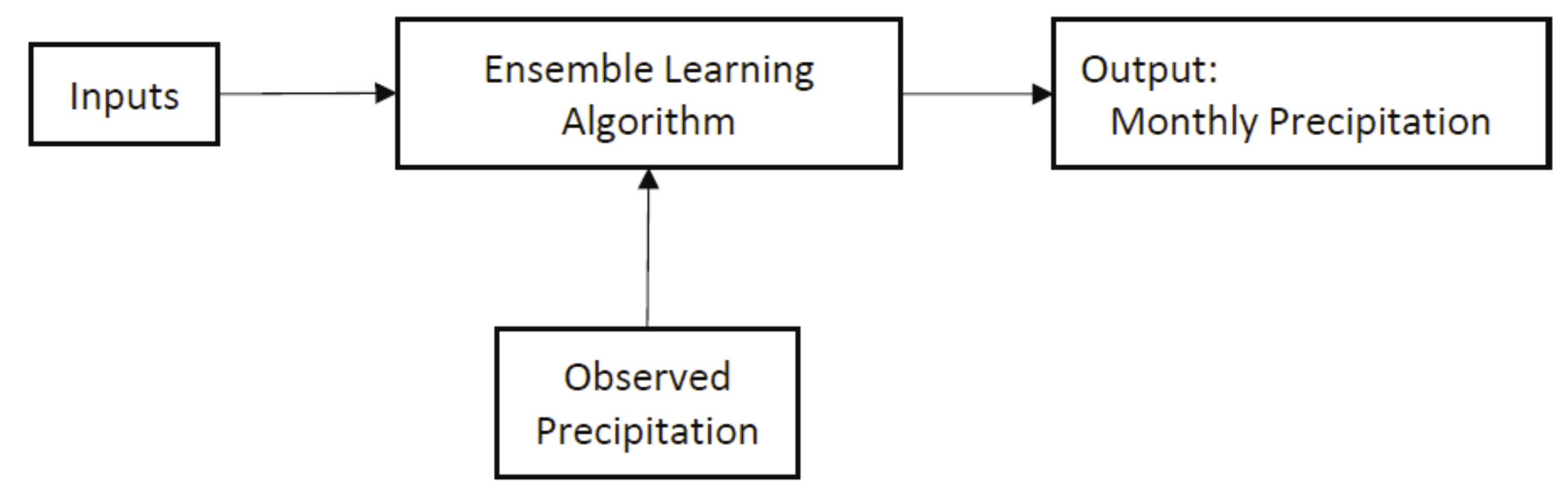
On the other hand, random forest (RF) is an ensemble method in machine learning that can be used for both classification and regression purposes. The base algorithm in RF is a decision tree (DT). Based on the type of the problem, two different types of DT are available: regression DT and classification DT. Thus, based on the type of DT, we can have RF for regression or classification. For more details about the RF, ANN, and DT, see [29]. In this paper, we used the machine learning toolbox of MATLAB 2018b. A general form of the proposed algorithm is depicted in Figure 3, wherein we will simply replace the ensemble learning algorithm by ANN or RF.
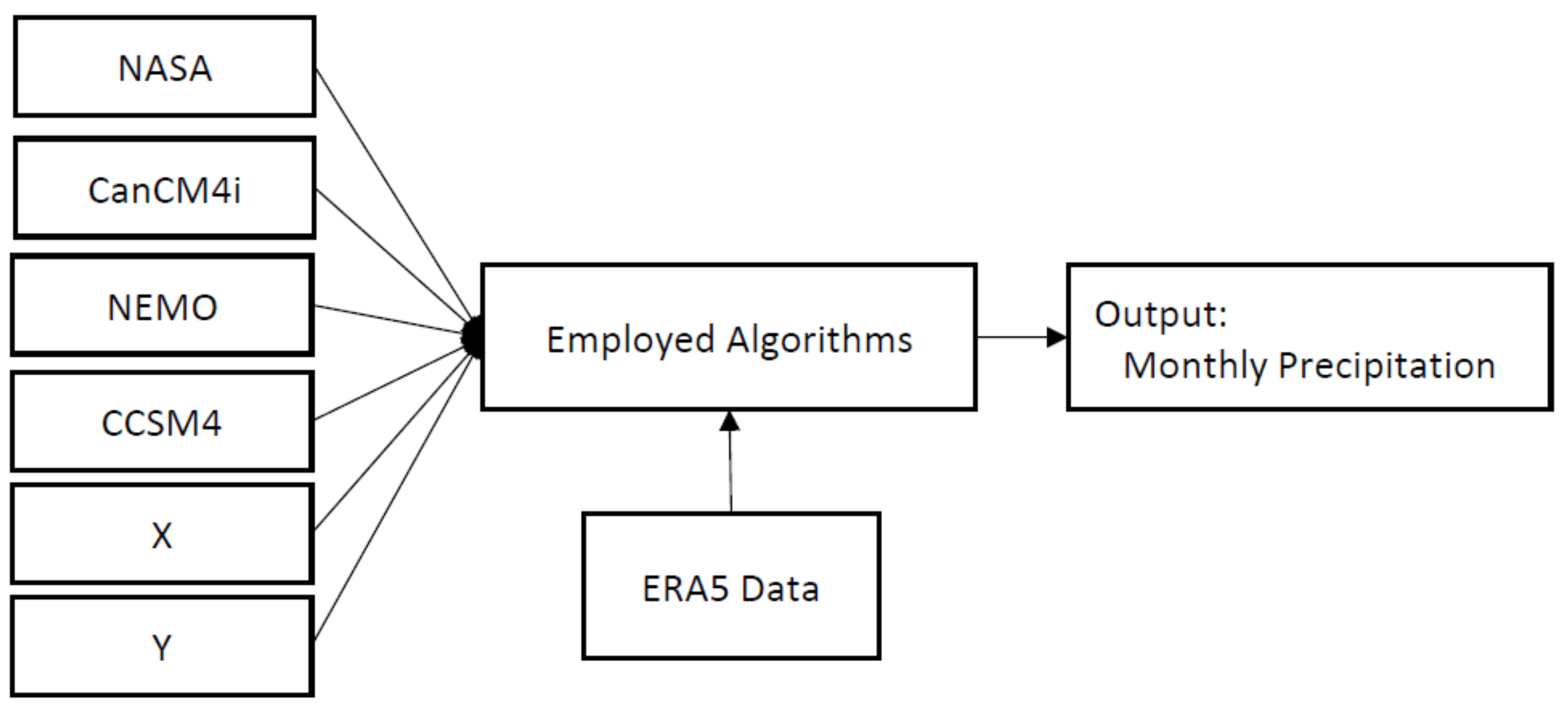
More details about the proposed approach are illustrated in Figure 4. As the figure shows, the proposed algorithm has six inputs and one output. The inputs include the monthly precipitation data of four models from the NMME project, along with the latitude and longitude of the region. In Figure 4, ERA5 data are used to train RF and ANN, and finally the output of the algorithm is an approximation of monthly precipitation.
Suppose that M is the output of the ANN or RF algorithm. Since each climate model generates the forecast data for different lead times, we need to construct a specific post-processing model related to each month and lead time. Suppose that is the output of the i-th NMME model M, for month m and lead time l. We can say that . Also suppose that, is the output of the RF or ANN algorithm for month m, and lead time l. Indeed, is a function of , , latitude, and longitude, as depicted in Figure 4. This function can be defined as follows:
wherein contains all data of , (four NMME models), and x and y indicate longitude and latitude, respectively. Furthermore, P indicates the adjustable parameters of RF or ANN. If F indicates the RF, P indicates the adjustable parameters of RF (for example the number of decision trees in the RF algorithm). If F indicates the ANN algorithm, P indicates the weights of input, hidden, and output layers of the ANN algorithm. The optimal values of P (which will be indicated by ) will be obtained for the training period. For a seasonal forecast, we do not need to provide separate RF and ANN algorithms. The monthly results of three consecutive months can be aggregated for the seasonal forecast of three months.
For selecting the correct initial months for each month for which the prediction is made, see Table 2. An example is provided in Table 3 for a situation which we have four lead times. This table indicates the correct month number for different initial months.
To compare the performance of the models, the values of the correlation coefficient, root mean squared error (RMSE), Kling–Gupta efficiency (KGE), and Nash–Sutcliffe efficiency (NSE) can be calculated as follows:
wherein M and O indicate the values of the model and observation, respectively. Furthermore, and denote the mean values of corresponding values. The can be calculated as follows:
Kling–Gupta efficiency (KGE) is defined as follows (see [30]):
wherein indicates the standard deviation. The maximum value of KGE is 1 which indicates perfect agreement between the model output and observations. Finally, the (Nash–Sutcliffe efficiency) is calculated as follows ([31]):
Similar to KGE, the maximum value of NSE is 1 which indicates perfect agreement between model output and observations.
For tuning the hyperparameters of the ANN and RF algorithms, we used an empirical approach. We examined several values for each hyperparameter and selected the best case. For example, to determine the best value for the number of decision trees in the RF, we examined the values 20, 40, 60, …, 200. The best performance of RF was achieved for the number of trees equal to 100. As another example, for the number of neurons in the hidden layer of the ANN, we examined the values 3, 6, 9, …, 21. The best performance of ANN (considering the RMSE, KGE, NSE, and the correlation coefficient) was achieved for the number of neurons equal to 15. It must be noted that using more (less) neurons or more (less) DTs may cause overfitting (underfitting).
4. Results and Discussion
4.1. Monthly Forecasts
After applying ANN and RF for post-processing the output of the four NMME models, the values of root mean squared error (RMS), correlation coefficient, Nash–Sutcliffe efficiency (NSE), and Kling–Gupta efficiency (KGE) were calculated to evaluate the performance of the proposed algorithms for each model separately.
The raw forecast performance of the four models (before post-processing), along with the performance of RF and ANN (after post-processing), was calculated for all lead times and months. To train and test the RF and ANN, the dataset was divided into two subsets. Since the hindcast period was 1982–2016 and contains 35 years, the period 1982–2007 (26 years) was considered for training the RF and ANN, while the period 2008–2016 (9 years) was considered to test the RF and ANN. This means that approximately 75% of data were used for training and 25% was used for testing.
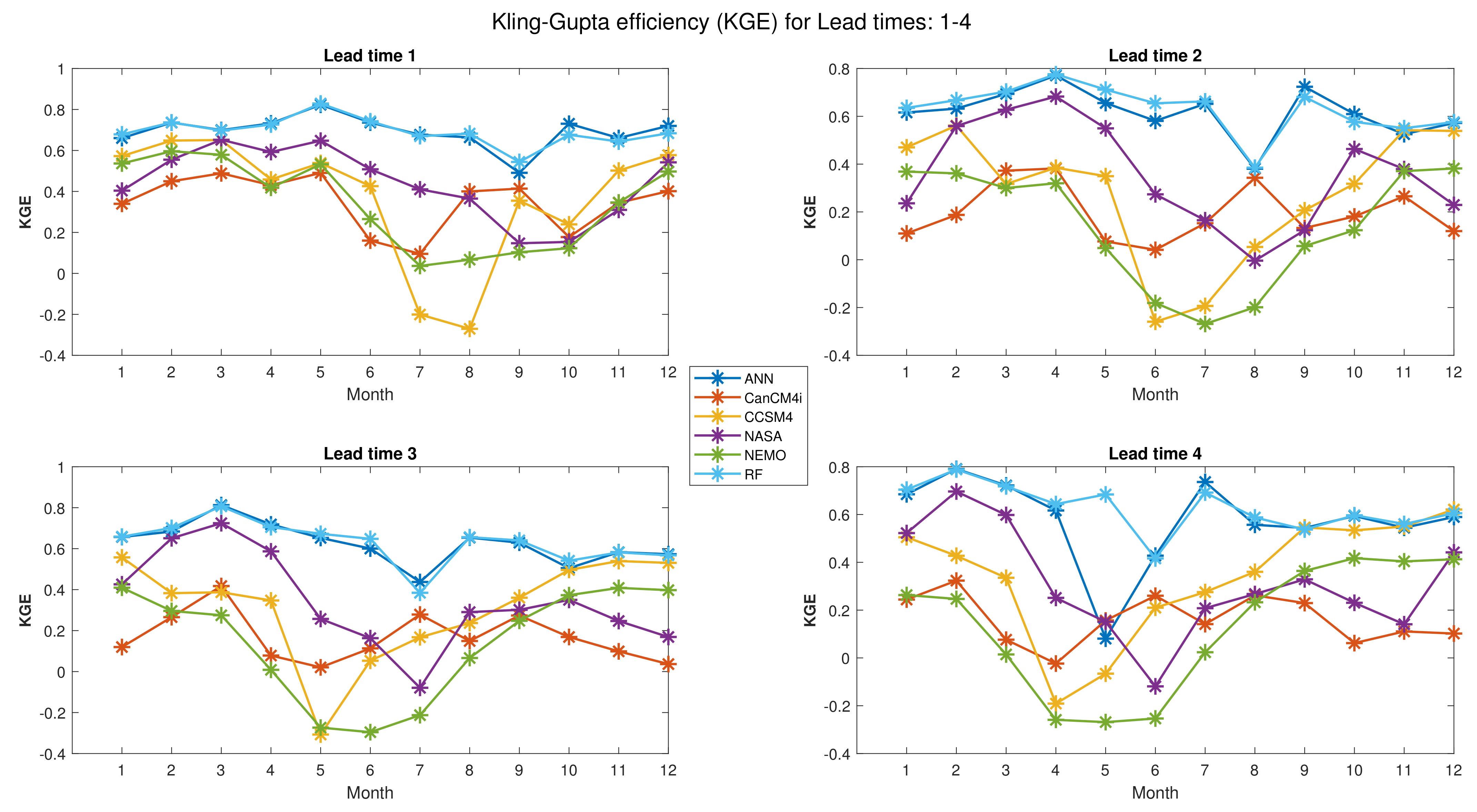
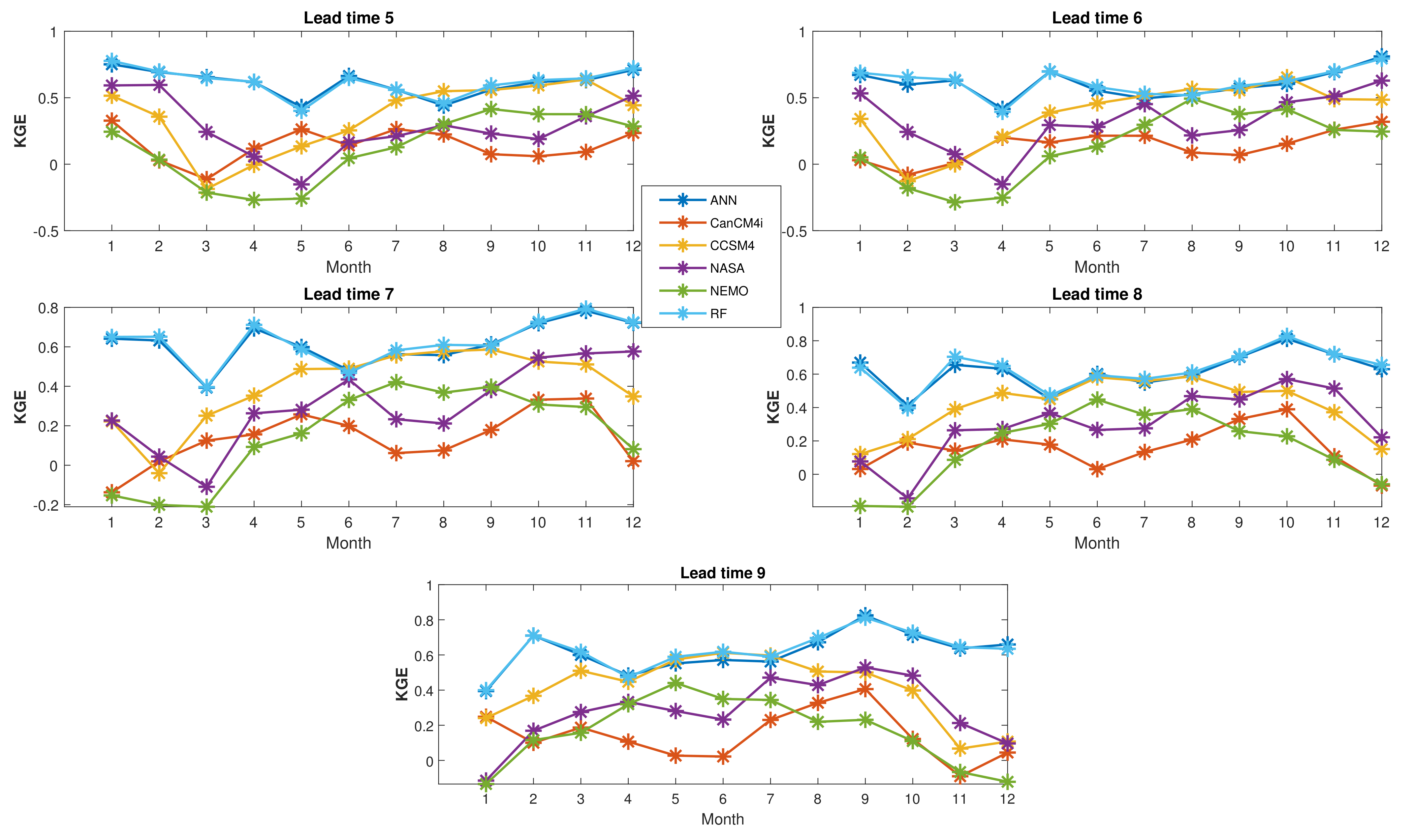
Figure 5 depicts the values of KGE for all months and lead times 1–4 while Figure 6 depicts the values of KGE for all months and lead times 5–9. For example, the maximum value of KGE in the first lead time of Figure 5 occurs in May (which predicts May itself) and for both ANN and RF. The maximum value of KGE in the second lead time of Figure 5 occurs in April (which predicts May) and for both ANN and RF. It is also should be noted that all calculated performance indices (KGE, RMSE, and NSE), as well as the correlation coefficient, were calculated for test period 2008–2016. Thus, all generated figures are devoted to period 2008–2016.
As shown in Figure 5, the values of KGE for RF and ANN are higher than the other NMME models. This is true for approximately all months and lead times (except May in lead 4, whereby the KGE of ANN is lower than that of NASA and CanCM4i). However, the values of KGE (for RF) for all months and lead times are higher than those for ANN and also the NMME models.
When considering the RF and ANN methods, Figure 5 shows that for lead time 1, the maximum forecast error occurs in September, which may be due to the fact that September is the transition month from the warm period to the cold period of the year. A similar discussion can be made for Figure 6. As shown in Figure 5, the lowest values of KGE for the NMME models are (for CCSM4 and month 8), (for NEMO and month 7), (for CCSM4 and month 5), and (for NEMO and month 5) for lead times 1–4, respectively. These values are improved by applying the RF method to , , , and respectively. Similarly, as shown in Figure 6, the lowest values of KGE for the NMME models are (for NEMO and month 4), (for NEMO and month 3), (for NEMO and month 3), (for NEMO and month 2), and (for NEMO and month 1) for lead times 5–9, respectively. These values are improved to (using the RF and ANN), (RF and ANN), (RF), (ANN), and (RF), respectively.
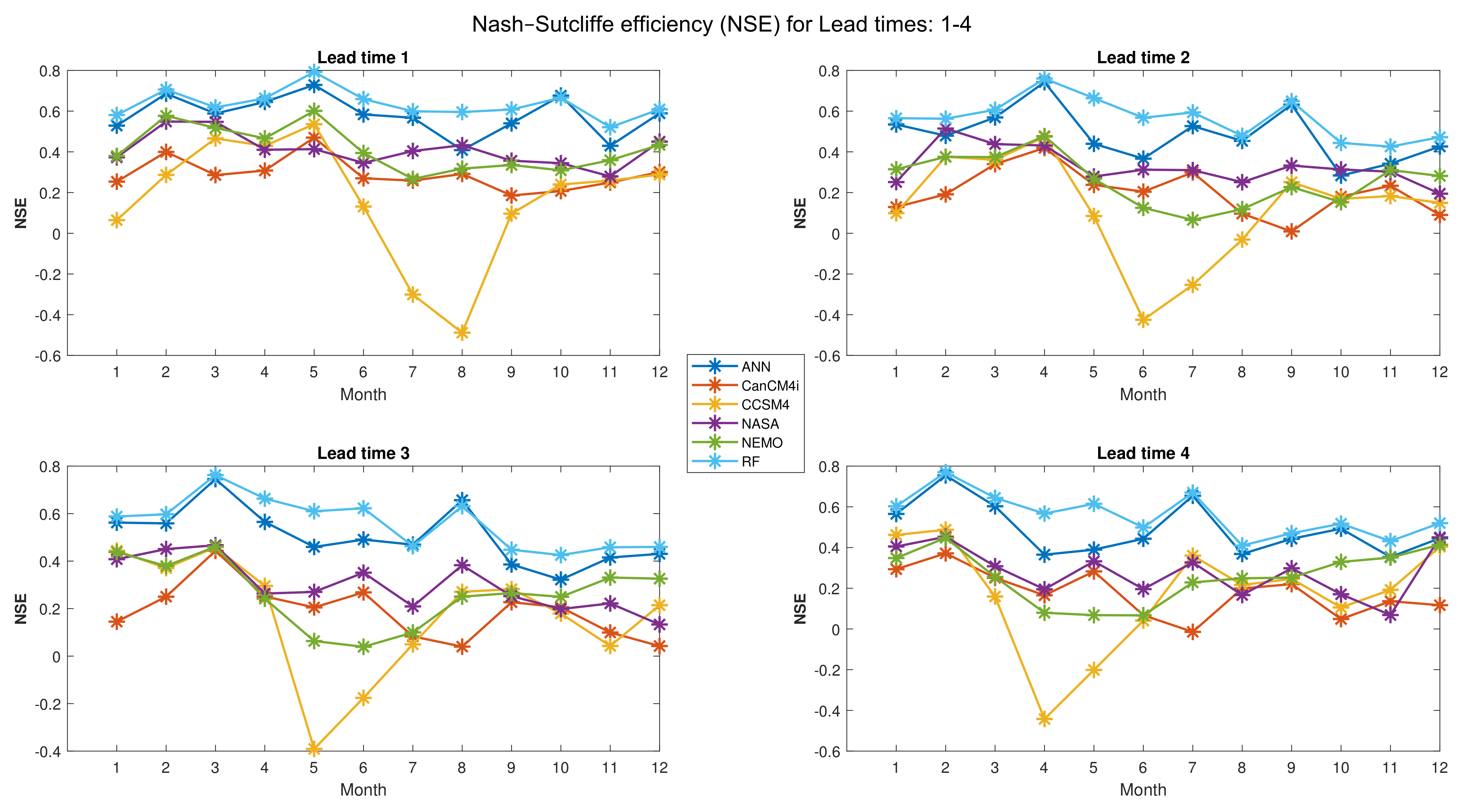
Figure 7 shows the values of NSE for all months and lead times 1–4. As it can be observed in Figure 7, the values of NSE for the RF and ANN are higher than those for the other NMME models. This is true for approximately all months and lead times (except some months of lead 2). However, the values of NSE for the RF algorithm (for all months and lead times) are higher than those for the ANN and also for the NMME models. As shown in Figure 7, the lowest values of NSE for the NMME models are (for CCSM4 and month 8), (for CCSM4 and month 6), (for CCSM4 and month 5), and (for CCSM4 and month 4) for lead times 1–4, respectively. These values are improved by the RF method to , , , and , respectively.
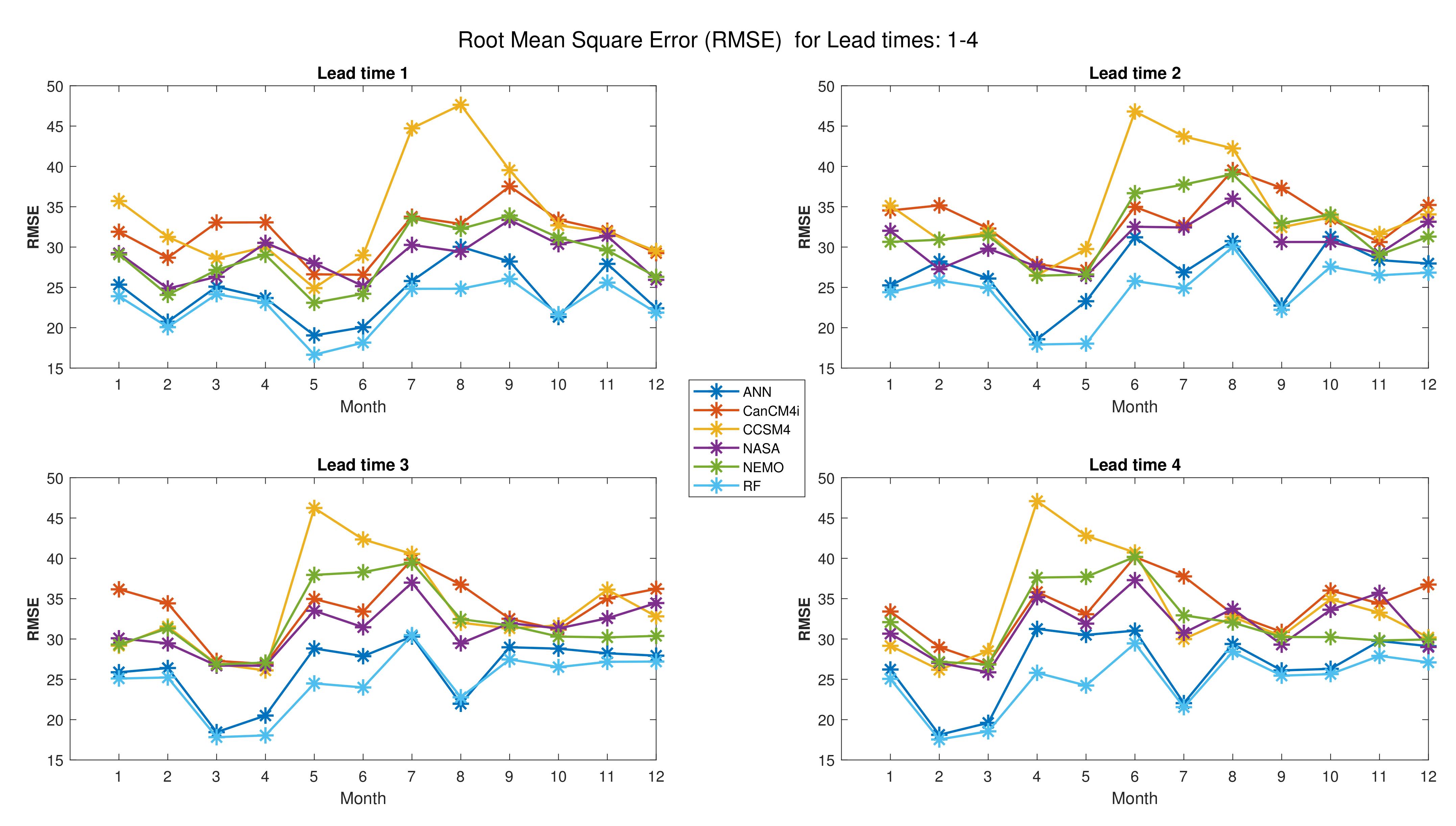
Figure 8 shows the values of RMSE for all months and lead times 1–4. As it can be observed in Figure 8, the values of RMSE for the RF and ANN are lower than those for the other NMME models. This is true for approximately all months and lead times. However, the values of RMSE for the RF algorithm (for all months and lead times) are lower than those for the ANN and also the NMME models. As shown in Figure 8, the maximum values of RMSE for the NMME models are (for CCSM4 and month 8), (for CCSM4 and month 6), (for CCSM4 and month 5), and (for CCSM4 and month 4) for lead times 1–4, respectively. These values are improved by the RF method to , , , and , respectively.
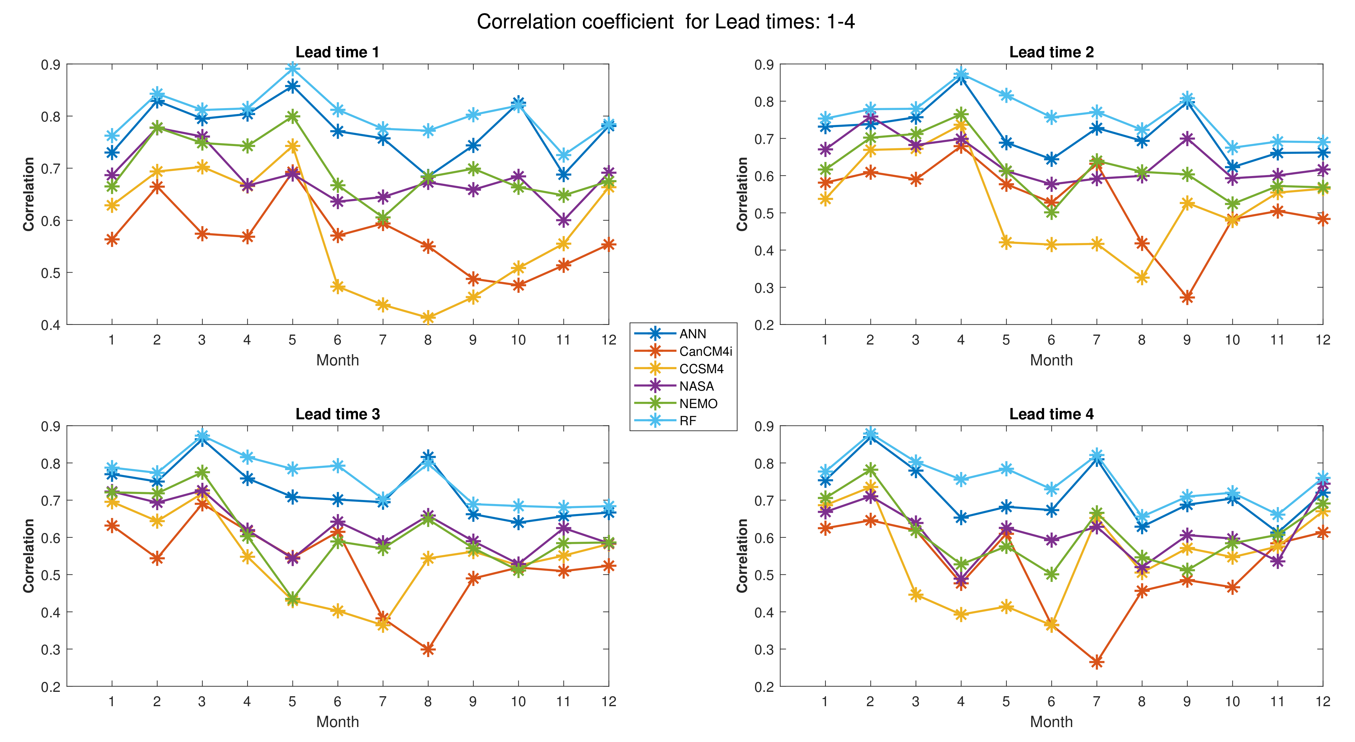
Figure 9 shows the values of correlation coefficient for all months and lead times 1–4. As it can be observed in Figure 9, the correlation coefficient values for the RF and ANN are higher than those for the other NMME models. This is true for approximately all months and lead times. However, the values of correlation coefficient for the RF algorithm (for all months and lead times) are higher than those for the ANN and also the NMME models. As shown in Figure 9, the lowest values of correlation coefficient for the NMME models are (for CCSM4 and month 8), (for CanCM4i and month 9), (for CanCM4i and month 8), and (for CanCM4i and month 7) for lead times 1–4, respectively. These values are improved to (RF), (RF), (ANN), and (RF), respectively.
4.2. Seasonal Forecasts
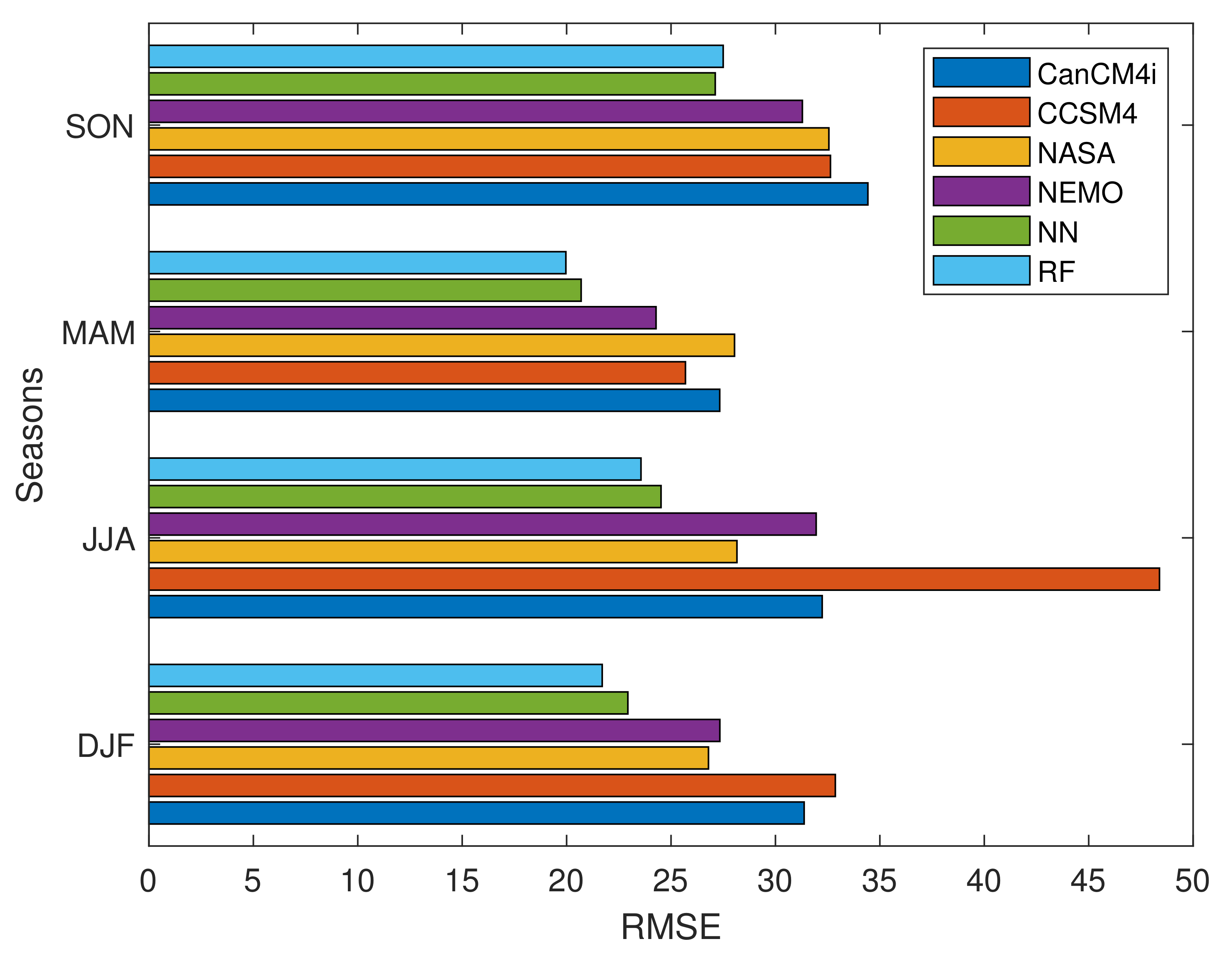
In this section, the skills of the proposed algorithm are evaluated for seasonal forecasts including: DJF (winter), MAM (spring), JJA (summer), and SON (autumn). For this purpose, the lead 1 data of three consecutive months were considered in order to generate the seasonal data. Similar calculations can be performed for the other lead times. Figure 10 depicts the values of RMSE for all seasons and for the test data (2008–2016). Except SON, whereby ANN has lower RMSE than RF, for other seasons, RF outperforms ANN. Furthermore, in comparison to four NMME models, the RMSE of ANN and RF is lower.
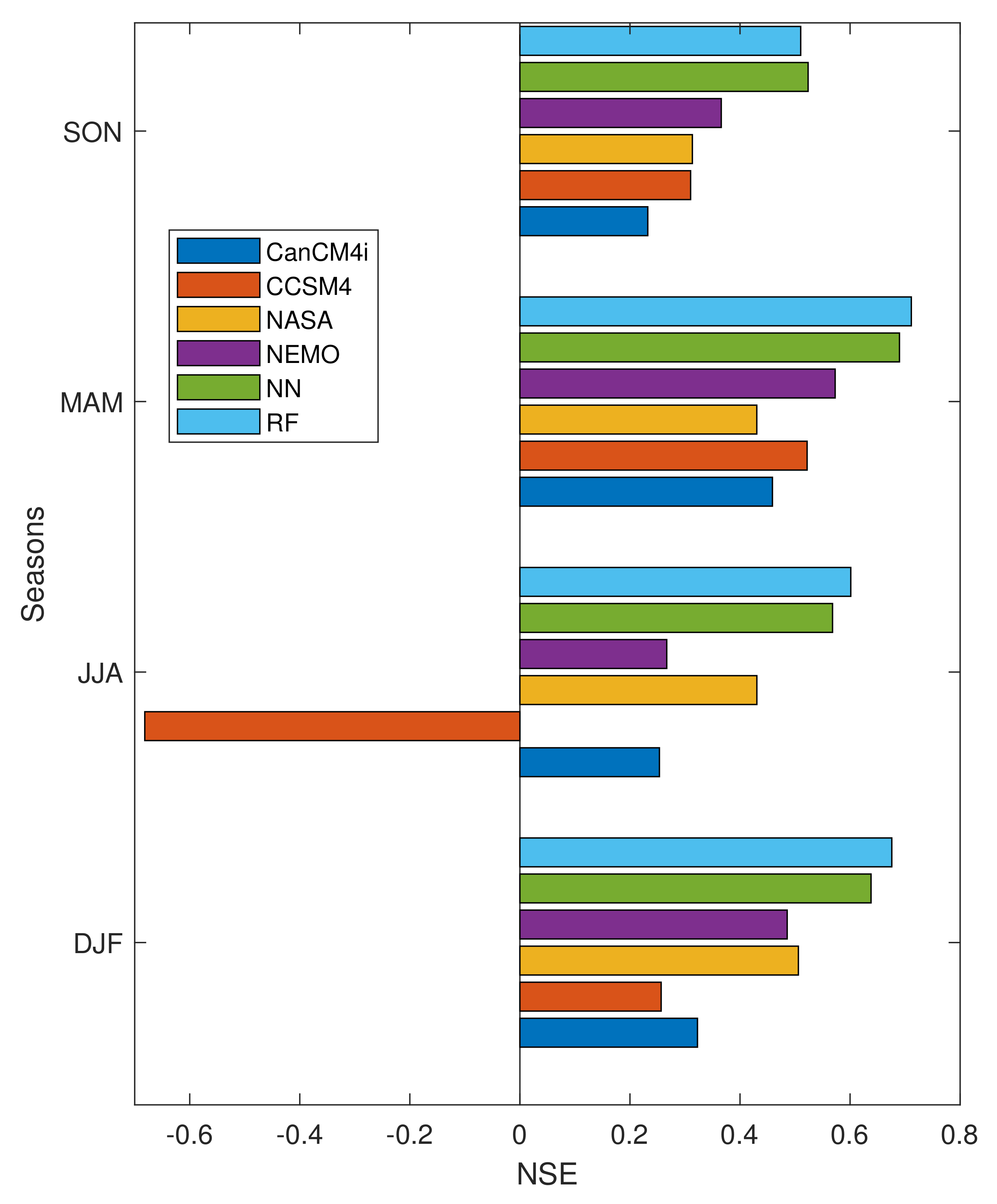
Figure 11 depicts the values of NSE for all seasons and for test data. Except SON, for which ANN has a larger NSE than RF, RF outperforms ANN. Moreover, in comparison with four NMME models, the values of NSE for ANN and RF are larger.
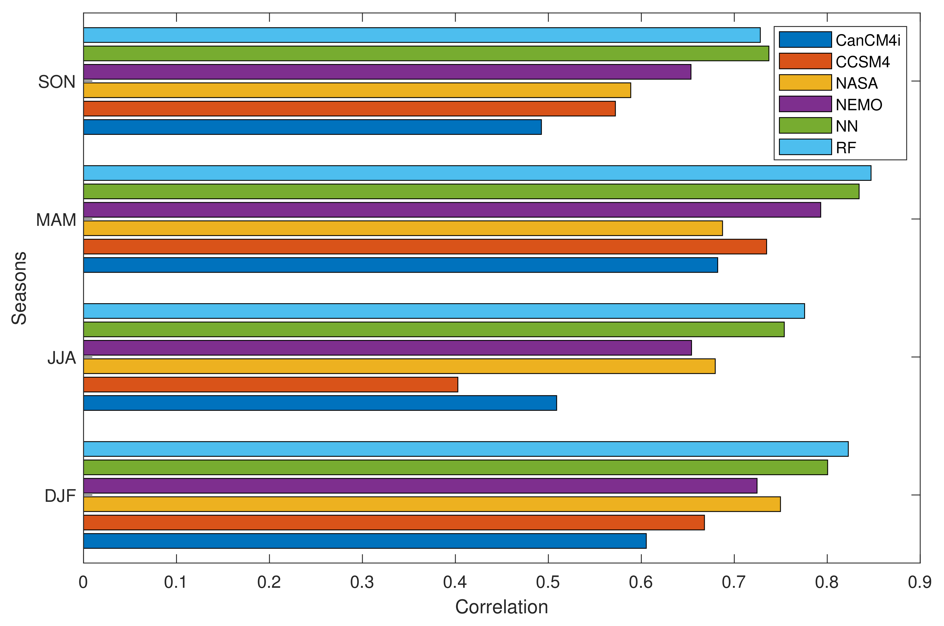
Figure 12 depicts the values of correlation coefficient for all seasons and for test data. Except SON, for which ANN has a larger correlation coefficient than RF, for other seasons, RF outperforms ANN. Furthermore, in comparison with four NMME models, the values of correlation coefficient for ANN and RF are larger.
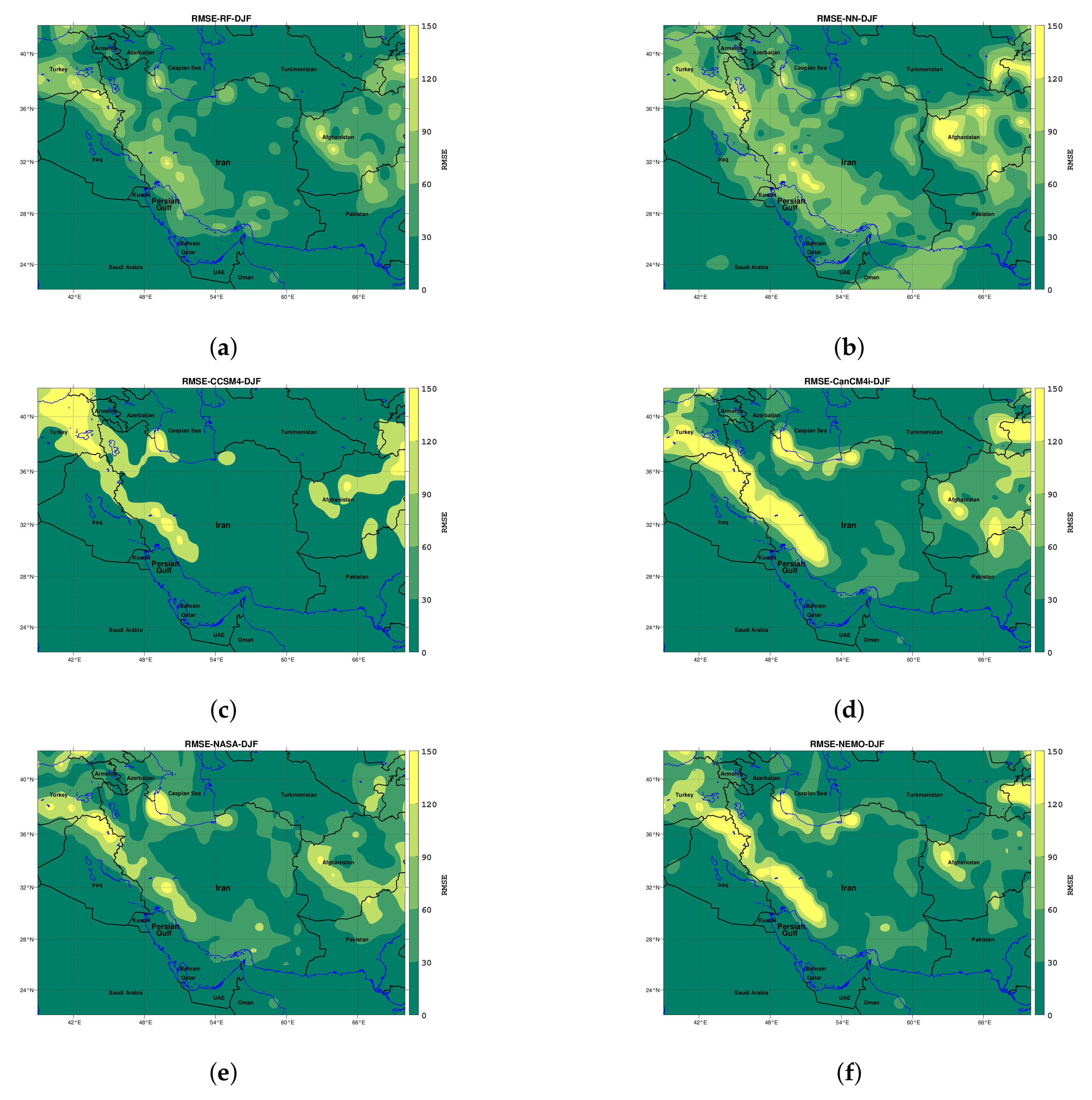
To indicate the performance pattern of the models, during the DJF season, the values of RMSE are plotted for test data in Figure 13. As it can be observed in Figure 13a, the RF algorithm has the best performance among the other models. After the RF algorithm, based on Figure 13b, the ANN algorithm has better performance in comparison with the NMME models. Moreover, it can be inferred that in the raw (NMME) model data, the maximum error occurs in the mountainous areas of Zagros and Alborz and lands in the east and south of the region. However, the ANN and RF methods are able to reduce the error over high-elevation lands, while the ability of the RF method to reduce the error is larger than that for the ANN. However, in both methods, the error increased slightly in some lowland areas.
5. Conclusions
In this paper, a multi-model ensemble approach was proposed for the monthly forecasting of precipitation using ANN and RF algorithms for southwest Asia. For this purpose, the outputs of four NMME models GEM-NEMO, NASA-GEOSS2S, CanCM4i, and COLA-RSMAS-CCSM4 were post-processed using the ERA5 data as a reference. The period 1982–2007 was used for learning the ANN and RF, while the data from period 2008–2016 were used for testing the algorithms. Since each model contains of nine different lead time, for each month of year, we had nine different datasets. In this paper, we trained 108 ANN and RF models for each lead time and month separately. Four performance evaluation criteria (root mean squared error (RMS), correlation coefficient, Nash–Sutcliffe efficiency (NSE), and Kling–Gupta efficiency (KGE), were calculated for each of 108 models along with NMME models. The results indicate that, approximately, the output of ANN and RF outperforms the NMME models for all months and lead times. Specifically, RF outperforms the ANN and the other four NMME models for all months and all lead times. The proposed algorithms and approach can be used for monthly forecasting precipitation in southwest Asia, but can also be modified for the monthly forecasting of, e.g., temperature and other variables. Moreover, other machine learning techniques could be applied to improve the accuracy of the proposed multi-model approach. The results of this research show that despite the vastness of the studied area and the different climates contained therein, machine learning methods can be used for post-processing and improving forecasts in a multi-model ensemble approach.
Author Contributions
Conceptualization, M.P. and I.B.; formal analysis, M.P. and I.B.; validation, M.P., I.B. and L.M.B.; writing—original draft preparation, M.P., I.B. and L.M.B.; writing—review and editing, M.P. and L.M.B.; funding acquisition, M.P. All authors have read and agreed to the published version of the manuscript.
Funding
This work was supported in part by the Iran National Science Foundation (INSF) under project number 98028362. L.M.B. was supported by the Helmholtz Association through the research programme Changing Earth—Sustaining our Future.
Data Availability Statement
The datasets that are analyzed in this paper are publicly available from the following archives: forecasting data from https://iridl.ldeo.columbia.edu (accessed on 22 January 2022); the ERA5 data from https://cds.climate.copernicus.eu (accessed on 22 January 2022).
Acknowledgments
We thank three anonymous reviewers for reading our paper, and for providing constructive comments that have helped to improve the presentation of our study.
Conflicts of Interest
The authors declare no conflict of interest.
Abbreviations
The following abbreviations are used in this manuscript:
| ANN | artificial neural network |
| DJF | December, January, February (winter) |
| ERA5 | ECMWF re-analysis dataset 5 |
| JJA | June, July, August (summer) |
| KGE | Kling–Gupta efficiency coefficient |
| MAM | March, April, May (spring) |
| NMME | North American multi-model ensemble |
| NSE | Nash–Sutcliffe efficiency coefficient |
| RF | Random forest |
| RMSE | Root mean squared error |
| SON | September, October, November (autumn) |
References
- Yazdi, H.S.; Pakdaman, M.; Effati, S. Fuzzy circuit analysis. Int. J. Appl. Eng. Res. 2008, 3, 1061–1072. [Google Scholar]
- Yuval, J.; O’Gorman, P.A. Stable machine-learning parameterization of subgrid processes for climate modeling at a range of resolutions. Nat. Commun. 2020, 11, 3295. [Google Scholar] [PubMed]
- Chang, F.J.; Hsu, K.; Chang, L.C. Flood Forecasting Using Machine Learning Methods; MDPI: Basel, Switzerland, 2019. [Google Scholar]
- Pakdaman, M.; Falamarzi, Y.; Babaeian, I.; Javanshiri, Z. Post-processing of the North American multi-model ensemble for monthly forecast of precipitation based on neural network models. Theor. Appl. Climatol. 2020, 141, 405–417. [Google Scholar]
- Pakdaman, M.; Babaeian, I.; Javanshiri, Z.; Falamarzi, Y. European Multi Model Ensemble (EMME): A New Approach for Monthly Forecast of Precipitation. Water Resour. Manag. 2022, 36, 611–623. [Google Scholar]
- Valipour, M. Optimization of neural networks for precipitation analysis in a humid region to detect drought and wet year alarms. Meteorol. Appl. 2016, 23, 91–100. [Google Scholar]
- Banadkooki, F.B.; Ehteram, M.; Ahmed, A.N.; Fai, C.M.; Afan, H.A.; Ridwam, W.M.; Sefelnasr, A.; El-Shafie, A. Precipitation forecasting using multilayer neural network and support vector machine optimization based on flow regime algorithm taking into account uncertainties of soft computing models. Sustainability 2019, 11, 6681. [Google Scholar]
- Scheuerer, M.; Switanek, M.B.; Worsnop, R.P.; Hamill, T.M. Using artificial neural networks for generating probabilistic subseasonal precipitation forecasts over California. Mon. Weather Rev. 2020, 148, 3489–3506. [Google Scholar]
- Das, S.; Chakraborty, R.; Maitra, A. A random forest algorithm for nowcasting of intense precipitation events. Adv. Space Res. 2017, 60, 1271–1282. [Google Scholar]
- Zarei, M.; Najarchi, M.; Mastouri, R. Bias correction of global ensemble precipitation forecasts by Random Forest method. Earth Sci. Inform. 2021, 14, 677–689. [Google Scholar]
- Shin, K.; Song, J.J.; Bang, W.; Lee, G. Quantitative Precipitation Estimates Using Machine Learning Approaches with Operational Dual-Polarization Radar Data. Remote Sens. 2021, 13, 694. [Google Scholar]
- Pakdaman, M.; Naghab, S.S.; Khazanedari, L.; Malbousi, S.; Falamarzi, Y. Lightning prediction using an ensemble learning approach for northeast of Iran. J. Atmos. Sol.-Terr. Phys. 2020, 209, 105417. [Google Scholar] [CrossRef]
- Pakdaman, M.; Falamarzi, Y.; Yazdi, H.S.; Ahmadian, A.; Salahshour, S.; Ferrara, F. A kernel least mean square algorithm for fuzzy differential equations and its application in earth’s energy balance model and climate. Alex. Eng. J. 2020, 59, 2803–2810. [Google Scholar] [CrossRef]
- Doughty, C.E.; Loarie, S.R.; Field, C.B. Theoretical impact of changing albedo on precipitation at the southernmost boundary of the ITCZ in South America. Earth Interact. 2012, 16, 1–14. [Google Scholar]
- Pakdaman, M.; Habibi Nokhandan, M.; Falamarzi, Y. Revisiting albedo from a fuzzy perspective. Kybernetes, 2021; ahead-of-print. [Google Scholar] [CrossRef]
- Han, X.; Wei, Z.; Zhang, B.; Li, Y.; Du, T.; Chen, H. Crop evapotranspiration prediction by considering dynamic change of crop coefficient and the precipitation effect in back-propagation neural network model. J. Hydrol. 2021, 596, 126104. [Google Scholar] [CrossRef]
- Aksoy, H.; Dahamsheh, A. Markov chain-incorporated and synthetic data-supported conditional artificial neural network models for forecasting monthly precipitation in arid regions. J. Hydrol. 2018, 562, 758–779. [Google Scholar]
- Chang, N.B.; Yang, Y.J.; Imen, S.; Mullon, L. Multi-scale quantitative precipitation forecasting using nonlinear and nonstationary teleconnection signals and artificial neural network models. J. Hydrol. 2017, 548, 305–321. [Google Scholar] [CrossRef]
- Tomassetti, B.; Verdecchia, M.; Giorgi, F. NN5: A neural network based approach for the downscaling of precipitation fields–Model description and preliminary results. J. Hydrol. 2009, 367, 14–26. [Google Scholar]
- Chen, H.; Chandrasekar, V.; Tan, H.; Cifelli, R. Rainfall estimation from ground radar and TRMM precipitation radar using hybrid deep neural networks. Geophys. Res. Lett. 2019, 46, 10669–10678. [Google Scholar] [CrossRef]
- Chen, G.; Wang, W.C. Short-term precipitation prediction for contiguous United States using deep learning. Geophys. Res. Lett. 2022, 49, e2022GL097904. [Google Scholar] [CrossRef]
- Shi, X. Enabling smart dynamical downscaling of extreme precipitation events with machine learning. Geophys. Res. Lett. 2020, 47, e2020GL090309. [Google Scholar] [CrossRef]
- Kim, J.W.; Pachepsky, Y.A. Reconstructing missing daily precipitation data using regression trees and artificial neural networks for SWAT streamflow simulation. J. Hydrol. 2010, 394, 305–314. [Google Scholar] [CrossRef]
- Hoell, A.; Cannon, F.; Barlow, M. Middle East and Southwest Asia daily precipitation characteristics associated with the madden–Julian oscillation during boreal winter. J. Clim. 2018, 31, 8843–8860. [Google Scholar] [CrossRef]
- Hoell, A.; Barlow, M.; Xu, T.; Zhang, T. Cold season southwest Asia precipitation sensitivity to El Niño–Southern Oscillation events. J. Clim. 2018, 31, 4463–4482. [Google Scholar] [CrossRef]
- Ehsan, M.A.; Kucharski, F.; Almazroui, M. Potential predictability of boreal winter precipitation over central-southwest Asia in the North American multi-model ensemble. Clim. Dyn. 2020, 54, 473–490. [Google Scholar] [CrossRef]
- Rana, S.; Renwick, J.; McGregor, J.; Singh, A. Seasonal prediction of winter precipitation anomalies over Central Southwest Asia: A canonical correlation analysis approach. J. Clim. 2018, 31, 727–741. [Google Scholar] [CrossRef]
- Cybenko, G. Approximation by superpositions of a sigmoidal function. Math. Control. Signals Syst. 1989, 2, 303–314. [Google Scholar] [CrossRef]
- Murphy, K.P. Machine Learning: A Probabilistic Perspective; MIT Press: Cambridge, MA, USA, 2012. [Google Scholar]
- Knoben, W.J.; Freer, J.E.; Woods, R.A. Inherent benchmark or not? Comparing Nash–Sutcliffe and Kling–Gupta efficiency scores. Hydrol. Earth Syst. Sci. 2019, 23, 4323–4331. [Google Scholar] [CrossRef]
- Nash, J.E.; Sutcliffe, J.V. River flow forecasting through conceptual models part I—A discussion of principles. J. Hydrol. 1970, 10, 282–290. [Google Scholar] [CrossRef]
Figure 1.
Region of study.

Figure 2.
General architecture of a single (hidden) layer perceptron neural network. f is the activation function.
Figure 2.
General architecture of a single (hidden) layer perceptron neural network. f is the activation function.

Figure 3.
A general architect of the proposed algorithm.

Figure 4.
Details of the proposed algorithm.

Figure 5.
Kling–Gupta efficiency (KGE) for lead times 1–4.

Figure 6.
Kling–Gupta efficiency (KGE) for lead times 5–9.

Figure 7.
Nash–Sutcliffe efficiency (NSE) for lead times 1–4.

Figure 8.
Root mean square error (RMSE) for lead times 1–4.

Figure 9.
Correlation coefficient for lead times 1–4.

Figure 10.
Seasonal RMSE for the models.

Figure 11.
Seasonal NSE for the models.

Figure 12.
Seasonal correlation coefficient for the models.

Figure 13.
The values of RMSE during the DJF for test data: (d–f) have the same range of RMSE in the color bar, unlike the other models in (a–c).
Figure 13.
The values of RMSE during the DJF for test data: (d–f) have the same range of RMSE in the color bar, unlike the other models in (a–c).


Table 1.
Four models which are used in this study for post-processing.
| Models | Abbreviation | Members | Lead Times | Hindcast Period |
|---|---|---|---|---|
| GEM-NEMO | NEMO | 10 | 12 (0.5–11.5 months) | 1981–2018 |
| NASA-GEOSS2S | NASA | 4 | 9 (0.5–8.5 months) | 1981–2017 |
| CanCM4i | CanCM4i | 10 | 12 (0.5–11.5 months) | 1981–2018 |
| COLA-RSMAS-CCSM4 | CCSM4 | 10 | 12 (0.5–11.5 months) | 1982–2021 |
Table 2.
Lead times versus months.
| Lead Time | 1 | 2 | … | 9 | |
|---|---|---|---|---|---|
| Month | |||||
| 1 | M(1,1) | M(1,2) | … | M(1,9) | |
| 2 | M(2,1) | M(2,2) | … | M(2,9) | |
| ⋮ | ⋮ | ⋮ | … | ⋮ | |
| 12 | M(12,1) | M(12,2) | … | M(12,9) | |
Table 3.
An example of determining the target month for a given month and lead time.
| Lead Time | L1 | L2 | L3 | L4 | |
|---|---|---|---|---|---|
| Month | |||||
| January | January | February | March | April | |
| February | February | March | April | May | |
| March | March | April | May | June | |
| April | April | May | June | July | |
| May | May | June | July | August | |
| June | June | July | August | September | |
| July | July | August | September | October | |
| August | August | September | October | November | |
| September | September | October | November | December | |
| October | October | November | December | January | |
| November | November | December | January | February | |
| December | December | January | February | March | |
Publisher’s Note: MDPI stays neutral with regard to jurisdictional claims in published maps and institutional affiliations. |
© 2022 by the authors. Licensee MDPI, Basel, Switzerland. This article is an open access article distributed under the terms and conditions of the Creative Commons Attribution (CC BY) license (https://creativecommons.org/licenses/by/4.0/).
Share and Cite
MDPI and ACS Style
Pakdaman, M.; Babaeian, I.; Bouwer, L.M. Improved Monthly and Seasonal Multi-Model Ensemble Precipitation Forecasts in Southwest Asia Using Machine Learning Algorithms. Water 2022, 14, 2632. https://doi.org/10.3390/w14172632
AMA Style
Pakdaman M, Babaeian I, Bouwer LM. Improved Monthly and Seasonal Multi-Model Ensemble Precipitation Forecasts in Southwest Asia Using Machine Learning Algorithms. Water. 2022; 14(17):2632. https://doi.org/10.3390/w14172632
Chicago/Turabian StylePakdaman, Morteza, Iman Babaeian, and Laurens M. Bouwer. 2022. "Improved Monthly and Seasonal Multi-Model Ensemble Precipitation Forecasts in Southwest Asia Using Machine Learning Algorithms" Water 14, no. 17: 2632. https://doi.org/10.3390/w14172632
Note that from the first issue of 2016, this journal uses article numbers instead of page numbers. See further details here.