Study on Critical Velocity of Sand Transport in V-Inclined Pipe Based on Numerical Simulation

Abstract

The Yellow River has a high sand content, and sand deposition in the pipelines behind the pumping station occurs from time to time. It is of great significance to reasonably predict the critical velocity of the small-angled V-inclined water transportation pipes. In this study, a Eulerian multiphase model was employed to simulate the solid–liquid two-phase flow. Based on the conservation of the sand transport rate, the critical velocity of the V-inclined pipe was predicted. The effects of simulated pipeline length, pipe inclination and particle size were investigated. The results show that when the simulated pipeline length reached a certain value, it did not affect the prediction of the critical velocity of the overall pipeline. The $\pm 2{}^{\circ }$ pipe inclination had a negligible effect on the critical velocity for transporting small-sized particles, but it led to the nonuniform and asymmetrical distribution of liquid velocity and sand deposition at the different cross-sections. As the particle size increased, the critical velocity also increased. However, the influence of particle size on the critical velocity is currently complicated, resulting in a large difference between numerical simulation and empirical formulas when transporting large-sized particles. Accurate prediction of critical velocity is important for long-distance water transportation pipelines to prevent sand deposition and reduce costs.

1. Introduction

The Yellow River in China is one of the rivers with the highest sand content in the world, containing a large proportion of small-sized suspended particles [1]. Due to the changes in the flow rate during the operation of the Yellow River long-distance water transportation pipelines, different degrees of sand deposition are produced in the pipelines. The characteristics of sand transport in the pipe can be described by the flow regime, which is divided into different velocities [2,3,4,5,6,7]. With a sufficiently high flow velocity, the sand can be completely suspended in the water, which can be considered as a homogeneous flow. However, if the flow velocity is low enough to reach a certain value, the sand separates from the water and the flow in the pipe becomes a heterogeneous flow. At an even lower flow velocity, the sand forms a moving bed at the bottom of the pipe and eventually a stationary deposition.

Scholars have conducted plenty of research on the velocities that delineate the different flow regimes, especially the critical velocity that triggers sand deposition at the bottom of the pipes [8,9,10,11]. Critical velocity is one of the most important parameters of pipelines, and it ensures the economic and safe operation of long-distance water transportation. In order to solve the sand deposition problem in the water transportation pipelines, the inflow velocity needs to be higher than the critical velocity. In practical engineering applications, the critical velocity law in the pipelines is extremely complex and affected by many factors. There are three main factors that affect the critical velocity: (1) pipe characteristics: pipe diameter and wall roughness; (2) fluid characteristics: slurry velocity and sand content; and (3) particle characteristics: particle size and particle grading composition, etc.

The critical velocity corresponds to the transition of the particle motion state. Since scholars focus on different particle motion states, the definitions of critical velocity are also distinct. Wasp [12], Shook [13] and Kokpinar [14] considered the critical velocity as the lowest point on the head loss and velocity curve of the pipe. Azamathulla [15] believed that the critical velocity is the value at which the flow velocity changes from small to large until there is no sand deposition at all. Durand [16], Thomas [17], Graf [18] et al. defined the critical velocity as the velocity from large to small until some particles begin to deposit, i.e., the minimum velocity at which all particles can remain in motion. According to He [19], the critical velocity is the average velocity of the cross-section when obvious bedload movement occurs in the pipe. An [20] considers the critical velocity as the average velocity of the cross-section when sand is pushed forward linearly and slowly at the bottom of the pipe without pile deposition. Although the above definitions of critical velocity are different, they are judged by the occurrence of sand deposition at the bottom of the pipes.

At present, there are two methods for predicting the critical velocity: an empirical formula and numerical simulation. Disagreement on the definition of critical velocity, differences in experimental measurement methods and differences in the hydraulic parameters chosen for the calculations lead to different empirical formulas. The representative ones are the formulas of Durand, Wasp, Shook, Turian and He Wuquan. However, the structural form of these formulas and the parameters involved vary greatly and are not universal. Compared with the empirical formulas obtained from experiments, numerical simulation has the advantage of being less expensive and more adaptable. Therefore, it is necessary to study critical velocity using numerical simulation. With the development of CFD, the numerical simulation of solid–liquid two-phase flow has been developed, and three-dimensional numerical simulation has greater advantages in analyzing local pipe sections. Sajeev [21] verified the accuracy of solid–liquid two-phase flow by numerical simulation in comparison with experiments. Ling [22] used a simplified ASM model to simulate the low-concentration solid–liquid two-phase flow. Kaushal [23] performed numerical simulations of pipeline slurry flow with mono-dispersed fine particles at high concentrations using Mixture and Eulerian two-phase models and found that the Eulerian model gives more accurate predictions for both the pressure drop and concentration profiles. Januário [24] used the CFD-DEM method to analyze characteristics of slurry flow at different velocities and compared this with the experiments. Dabirian [25] numerically simulated the critical velocity and compared it with experiments to investigate the effects of parameters such as particle size and fluid viscosity on sand transport in horizontal pipelines and to illustrate the feasibility of numerical simulation predictions of critical velocity. Yang [26] investigated the transport and deposition characteristics of sand in the pipeline by means of the Eulerian multiphase flow model and examined the effects of inlet velocity, particle size and sand concentration.

Long-distance water transportation pipelines unavoidably follow undulating topography. Although the bending angle is small, it complicates the multiphase flow. Most studies have focused on the flow in horizontal pipes and other forms of inclined pipes. Therefore, it is of great significance to study the critical velocity of V-inclined pipe with a small bend angle. Al-lababidi [27] compared a horizontal pipe with a +5° upward-inclined pipe and found that the pipe inclination had a negligible effect on the critical velocity but a significant effect on the sand transport. Danielson [28] studied the sand transport in −1.35° and +4° upward-inclined pipes in liquid and liquid–gas flow and found that the pipe inclination had no significant effect on the sand transport in liquid. Dabirian [29] experimentally investigated the effect of parameters such as particle size, sand content and phase velocity on the three-phase flow of a +1.5° upward-inclined pipe. Conversely, Tebowei et al. [30] used the Eulerian–Eulerian two-fluid model to simulate the sand transport in the V-inclined pipeline. They found that the small-angled V-inclined pipe had a significant impact on sand disposition compared to the horizontal section, and the critical velocity was much higher at the downstream section of the V-inclined pipe. Nossair [31] experimentally studied a +3.6° upward-inclined pipe and found that a higher flow rate is required to eliminate sand deposition in small-angle upward-inclined pipe compared to horizontal pipe. Stevenson [32] reported that downward-inclined pipe is more prone to sand deposition than upward-inclined pipe. Wang [33] used a single variable to conduct experimental research on an inclined pipe. They found that there is an optimal angle between the horizontal and inclined pipes, which makes the critical velocity have a maximum value. They also modified Wasp’s empirical formula to obtain the critical velocity of the inclined pipe. V-inclined pipes tend to be affected by the curvature of the pipe and require more attention compared to separate upward- and downward-inclined pipes.

In this paper, a three-dimensional numerical simulation of a small-angle V-slope water transportation pipe was performed to predict the critical velocity of the pipe based on the conservation of the sand transport rate. The accuracy of the numerical simulation was verified by comparing it with the empirical formula. The effect of simulated pipeline length, pipe inclination and particle size on the critical nonsiltation flow velocity was investigated by controlling a single variable.

2. Numerical Method

2.1. Governing Equations

In the solid–liquid two-phase flow, the water is the primary phase while the sand is the secondary phase. The Eulerian multiphase model was employed to predict the solid–liquid two-phase flow in the pipe [26,30,34,35].The model treats each phase as a continuous medium in time and space, existing in the same space and permeating each other. However, each phase has different volume fraction velocities, temperatures and densities. There is slip and interaction between phases. Momentum and continuity equations are solved for each phase. The following is the governing equation of the Eulerian model applicable to multiphase flow.

The description of multiphase flow as interpenetrating continua incorporates the concept of phasic volume fractions, denoted here by ${\alpha }_q$.

$$\sum _{q=1}^n{\alpha }_q=1$$

(1)

The solid phase is represented by s, the liquid phase is represented by l, ${\alpha }_{{}_s}$ and ${\alpha }_{{}_l}$ is the volume fraction of the liquid phase and the solid phase respectively, then:

$${\alpha }_{{}_s}+{\alpha }_l=1$$

(2)

The conservation of the mass equation for phase q is:

$$\frac{\partial }{\partial \mathrm{t}}\left({\alpha }_q{\rho }_q\right)+\nabla ·\left({\alpha }_q{\rho }_q{\mathit{v}}_q\right)=\sum _{p=1}^n\left({\dot{m}}_{pq}-{\dot{m}}_{qp}\right)$$

(3)

where ${\rho }_q$ is the physical density of phase q, ${\mathit{v}}_q$ is the velocity of phase q, ${\dot{m}}_{qp}$ characterizes the mass transfer from phase q to phase p, and ${\dot{m}}_{pq}$ characterizes the mass transfer from phase p to phase q, and t is time.

In this study, there was no mass transfer between the solid and liquid phases, so ${\dot{m}}_{qp}$ and ${\dot{m}}_{pq}$ are both 0, and Equation (3) was simplified as:

$$\frac{\partial }{\partial \mathrm{t}}\left({\alpha }_q{\rho }_q\right)+\nabla ·\left({\alpha }_q{\rho }_q{v}_q\right)=0$$

(4)

The conservation of momentum equation for phase q is:

$$\begin{array}{cc}\hfill \frac{\partial }{\partial \mathrm{t}}\left({\alpha }_q{\rho }_q{\mathit{v}}_q\right)+\nabla ·\left({\alpha }_q{\rho }_q{\mathit{v}}_q{\mathit{v}}_q\right)=& -{\alpha }_q\nabla p+\nabla ·{\overline{\overline{\tau }}}_q+{\alpha }_q{\rho }_q\mathit{g}\hfill \\ & +\sum _{p=1}^n\left({\mathit{R}}_{pq}+{\dot{m}}_{pq}{\mathit{v}}_{pq}-{\dot{m}}_{qp}{\mathit{v}}_{qp}\right)\hfill \\ & +\left({\mathit{F}}_q+{\mathit{F}}_{lift,q}+{\mathit{F}}_{wl,q}+{\mathit{F}}_{vm,q}+{\mathit{F}}_{td,q}\right)\hfill \end{array}$$

(5)

where ${\overline{\overline{\tau }}}_q$ is the qth-phase stress–strain tensor:

$${\overline{\overline{\tau }}}_q={\alpha }_q{\mu }_q\left(\nabla {\mathit{v}}_q+\nabla {{\mathit{v}}_q}^T\right)+{\alpha }_q\left({\lambda }_q-\frac{2}{3}{\mu }_q\right)\nabla ·{\mathit{v}}_q\overline{\overline{I}}$$

(6)

where g is the acceleration of gravity, ${\mu }_q$ and ${\lambda }_q$ are the shear and bulk viscosity of phase q, $\overline{\overline{I}}$ is the unit tensor, ${\mathit{F}}_q$ is an external body force, ${\mathit{F}}_{lift,q}$ is a lift force, ${\mathit{F}}_{wl,q}$ is a wall lubrication force, ${\mathit{F}}_{vm,q}$ is a virtual mass force, ${\mathit{F}}_{td,q}$ is a turbulent dispersion force, and p is the pressure shared by all phases. ${\mathit{R}}_{pq}$ is an interaction force between phases. ${\mathit{v}}_{pq}$ and ${\mathit{v}}_{qp}$ are the interphase velocities.

This paper considered the effect of gravity on sand deposition. Only the interaction force was considered between phases, ignoring the forces that have less influence such as lift force and virtual mass force. Equation (5) can be simplified as:

$$\frac{\partial }{\partial \mathrm{t}}\left({\alpha }_q{\rho }_q{v}_q\right)+\nabla ·\left({\alpha }_q{\rho }_q{v}_q{v}_q\right)=-{\alpha }_q\nabla p+\nabla ·{\overline{\overline{\tau }}}_q+{\alpha }_q{\rho }_{q}g+{\mathit{R}}_{pq}$$

(7)

For solid–liquid two-phase flow, the interaction force uses the Wen-Yu model and satisfies ${\mathit{R}}_{ls}=-{\mathit{R}}_{sl}$:

$${\mathit{R}}_{ls}=\frac{3{\alpha }_s{\alpha }_l{\rho }_l\left|{\mathit{v}}_s-{\mathit{v}}_l\right|}{4d_s}{{\alpha }_l}^{-2.65}·\frac{24}{{\alpha }_{l}R{e}_f}[1+0.15{\left({\alpha }_{l}R{e}_f\right)}^{0.687}]·({\mathit{v}}_l-{\mathit{v}}_s)$$

(8)

where $d_s$ is the diameter of the solid phase; and $R{e}_f$ is the relative Reynolds number.

2.2. Turbulence Model

Three turbulence models are used to simulate turbulence in multiphase flows: the mixture turbulence model, the dispersed turbulence model and a per-phase turbulence model. These models were used by Kaushal [23], Li [34] and Ekambara [36], respectively. The choice of turbulence model is based on the importance of the second-phase turbulence. The mixture turbulence model uses mixture properties and mixture velocities, which are sufficient to capture important features of the turbulent flow. Therefore, it was also used in this study to reduce the computational overhead while meeting the accuracy requirements of the calculation.

The turbulence kinetic energy k and its rate of dissipation $\epsilon$ are obtained from the following transport equations:

$$\frac{\partial }{\partial t}\left({\rho }_{m}k\right)+\nabla ·\left({\rho }_m{\mathit{v}}_{m}k\right)=\nabla ·\left(\left({\mu }_m+\frac{{\mu }_{t,m}}{{\sigma }_k}\right)\nabla k\right)+G_{k,m}-{\rho }_m\epsilon$$

(9)

$$[\frac{\partial }{\partial t}\left({\rho }_m\epsilon \right)+\nabla ·\left({\rho }_m{\mathit{v}}_m\epsilon \right)=\nabla ·\left(\left({\mu }_m+\frac{{\mu }_{t,m}}{{\sigma }_{\epsilon }}\right)\nabla \epsilon \right)+\frac{\epsilon }{k}\left(C_{1\epsilon }{G}_{k,m}-C_{2\epsilon }{\rho }_m\epsilon \right)]$$

(10)

where ${\sigma }_k$ and ${\sigma }_{\epsilon }$ are the turbulent Prandtl numbers for k and $\epsilon$, respectively. $C_{1\epsilon }$ and $C_{2\epsilon }$ are constants.

$G_{k,m}$, the generation of turbulence kinetic energy, is described as:

$$G_{k,m}={\mu }_{t,m}\left(\nabla {\mathit{v}}_m+{\left(\nabla {\mathit{v}}_m\right)}^T\right):\nabla {\mathit{v}}_m$$

(11)

The turbulent viscosity ${\mu }_{t,m}$ for the mixture can be expressed as:

$${\mu }_{t,m}={\rho }_m{C}_{\mu }\frac{k^2}{\epsilon }$$

(12)

where $C_{\mu }$ is a constant.

The mixture density ${\rho }_m$, velocity ${\mathit{v}}_m$ and molecular viscosity ${\mu }_m$ are listed below:

$${\rho }_m=\sum _{i=1}^N{\alpha }_i{\rho }_i$$

(13)

$${\mathit{v}}_m=\frac{{\displaystyle \sum _{i=1}^N}{\alpha }_i{\rho }_i{\mathit{v}}_i}{{\displaystyle \sum _{i=1}^N}{\alpha }_i{\rho }_i}$$

(14)

$${\mu }_m=\sum _{i=1}^N{\alpha }_i{\mu }_i$$

(15)

where ${\alpha }_i$, ${\rho }_i$, ${\mu }_i$ and $v_i$ are the volume fraction, density, viscosity and velocity of the ith phase, respectively.

2.3. Computational Domain and Grid-Independent Analysis

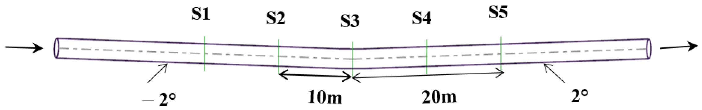
The typical small-angled V-inclined pipe in the pipeline irrigation project of the Yellow River irrigation area was used as the research object. It consisted of −2° downward-inclined pipe and +2° upward-inclined pipe, as shown in Figure 1. The prototype size was used for three-dimensional modeling. The pipe diameter and length were 2600 mm and 80 m, respectively. The sections denoted S1, S2, S3, S4 and S5 on the pipe, as shown in the figure, are the cross-sections where the predicted data were obtained for analysis. Sand deposition at different inflow velocities can be observed in these cross-sections. S3 was the section where the lowest point of the pipe was located. S1, S2, S4 and S5 were located at −20 m, −10 m, 10 m and 20 m, respectively, from the S3 section.

In the study of sand transport and deposition characteristics of multiphase flow, the grid is an important factor affecting the numerical simulation. The coarse mesh of 764,000 cells, the medium mesh of 1,487,600 cells, and the fine mesh of 1,855,600 cells were employed to analyze the sensitivity of the grid resolution to the numerical simulation results, as shown in Figure 2. Considering the influence of wall roughness on the sand deposition, five boundary layers were established along the surface with a growth factor of 1.2, and the height of the first layer from the wall was 5 mm.

The slurry velocity at the S3 cross-section was chosen to evaluate the effect of the grid number on the flow characteristics. Numerical simulations were carried out at an inlet volume fraction of 0.42% and an inlet velocity of 0.3 m/s.

Table 1. Slurry velocity at the S3 cross-section under different grid numbers.

Scheme Number	Grid Number	Slurry Velocity (m/s)	Relative Error (%)
1	764,000	0.3029	0.66
2	1,487,600	0.3010	0.03
3	1,855,600	0.3009	0

shows the slurry velocity at the S3 cross-section for different grid numbers and the relative errors between them. Considering the computational time and accuracy, the final numerical simulation of the multiphase flow was carried out with a grid number of 1,487,600.

2.4. Solution Strategies and Boundary Conditions

The ANSYS FLUENT software was used as a computational platform. The pressure and velocity equations were coupled using a phase-coupled SIMPLE algorithm. The continuity, momentum and turbulence equations were discretized by the second-order upwind scheme, while the volume fraction equation was discretized by the first-order upwind. Velocity and volume fraction of liquid and solid phases were assigned at the inlet condition of this pipe. The pressure was specified at the outlet condition of this pipe. The turbulence specification method used the intensity and hydraulic diameter. At the wall, the velocity was set to zero, which corresponds to the no-slip condition.

The literature shows that the particle size has a greater effect on critical velocity than bed roughness [37]. In the numerical simulation, the roughness of the pipe was not considered. The liquid phase was regarded as an incompressible fluid, and the physical properties of the solid phase were all constants, without considering the phase transformation. The shapes comprising the solid phase were treated as spherical particles of the same size.

Table 2. Parameters under different simulation conditions.

Parameters	Horizontal Pipe	V-Inclined Pipe
		±2°
Grid cell size (m)	0.05	0.05
Pipe length L (m)	80	80/150/200
Pipe diameter D (mm)	2600	2600
Liquid density $\rho$ ($\mathrm{kg}·{\mathrm{m}}^{-3}$ )	998.2	998.2
Sand density ${\rho }_s$ ($\mathrm{kg}·{\mathrm{m}}^{-3}$)	2300	2300
Particle size d (mm)	0.02	0.02\0.05\0.1
Sand content $C_s$ ($\mathrm{kg}·{\mathrm{m}}^{-3}$)	9.71	9.71
Sand volume concentration $C_V$ (%)	0.42	0.42
Inflow velocities (m/s)	0.3–0.7	0.3–1.6

shows parameters under different simulation conditions.

The numerical simulation method for solid–liquid two-phase flow used in this paper was validated by previous experiments [23,26]. The prediction of the critical velocity was achieved by setting different inflow velocities.

3. Results and Discussion

3.1. Comparison between Empirical Formula and Numerical Simulation

Many scholars have summarized the empirical formula of critical velocity in horizontal pipe through experiments. In this study, the critical velocity was predicted by numerical simulation based on the conservation of the sand transport rate. To verify the accuracy, a numerical simulation of the horizontal pipe was carried out and compared with the critical velocity obtained by the empirical formula.

3.1.1. Empirical Formula for Critical Velocity

There are differences in the definition and experimental measurement methods of critical velocity, resulting in different empirical formulas. The factors affecting the critical flow rate generally include sand content, particle size, pipe diameter, pipe roughness, etc. The representative empirical formulas are shown in

Table 3. Empirical formula of critical velocity for horizontal pipe.

Reference	Empirical Formula
Durand [16]	$v_c=F_L{\left(2gD\frac{{\rho }_s-\rho }{\rho }\right)}^{\frac{1}{2}}$
Wasp [12]	$v_c=3.28{C_V}^{0.243}{\left(2gD\frac{{\rho }_s-\rho }{\rho }\right)}^{\frac{1}{2}}{\left(\frac{d}{D}\right)}^{\frac{1}{6}}$
Shook [13]	$v_c=2.43\frac{{C_V}^{\frac{1}{3}}}{{C_D}^{\frac{1}{4}}}{\left(2gD\frac{{\rho }_s-\rho }{\rho }\right)}^{\frac{1}{2}}$
He Wuquan [19]	$v_c=1.8644K{C_W}^{0.2341}{\left(gD{\omega }^2\frac{{\rho }_s-\rho }{\rho }\right)}^{\frac{1}{4}}$

.

In Table 3 $F_L$ is the modified Froude number when the solid particles appear to settle and thus deposit, which needs to be measured experimentally. $C_D$ is the drag coefficient, $\omega$ is the settling velocity of particles, K is the correction factor, and the self-pressure pipe is taken as 1.05.

It can be seen from Table 3 that the empirical formulas based on experiments have similar structural characteristics, but the exponents and coefficients of each parameter are quite different. In most formulas, the critical velocity has an exponential relationship with the pipe diameter, and the critical velocity increases with the increase in the pipe diameter. At the same time, there is an exponential relationship between the critical velocity and sand content $v_c\propto {C_V}^m\left(0<m<1\right)$. Many studies have shown that the critical velocity increases with the increase in the sand content. When a certain limit is reached, the critical velocity decreases. There is a limit value between the critical velocity and the sand content. On the one hand, the increase in sand content inhibits the turbulent intensity of the liquid, and on the other hand, it increases the viscosity between particles and reduces the settling velocity of particles. However, the relationship between critical velocity and particle size is different. The particle size is not included in the formula of Shook. The critical velocity in the formula of Wasp is proportional to the particle size. Although the formula of He Wuquan does not contain particle size, the settling velocity in the formula is proportional to the particle size. It can be seen that the relationship between critical velocity and particle size is complicated.

3.1.2. Numerical Simulation for Critical Velocity

The empirical formula of critical velocity is influenced by experimental measurements as well as the measured parameters, and thus has poor applicability and reliability. Numerical simulation can be used to predict the critical velocity under different conditions, which is more economical.

The movement of sand in the pipelines of the Yellow River irrigation area is dominated by suspension movement, and sand deposition does not easily occur. However, due to the change in flow rate during operation, the sand deposition will occur when the flow rate is too low to maintain the suspension movement of sand. In this paper, critical velocity in the pipe was predicted based on the conservation of the sand transport rate. If the inlet and outlet mass flow rate of sand is basically equal, that is, the net mass flow rate is close to 0, the sand volume concentration no longer changes with time and sand in the pipe reaches the equilibrium between transport and deposition at that inflow velocity. In this paper, it was considered that on the premise of reaching the equilibrium between transport and deposition, the minimum inflow velocity at which the sand volume concentration does not increase with time is the critical velocity of the pipe. At the critical velocity, the sand moves slowly at the bottom of the pipe, but it will not accumulate in piles.

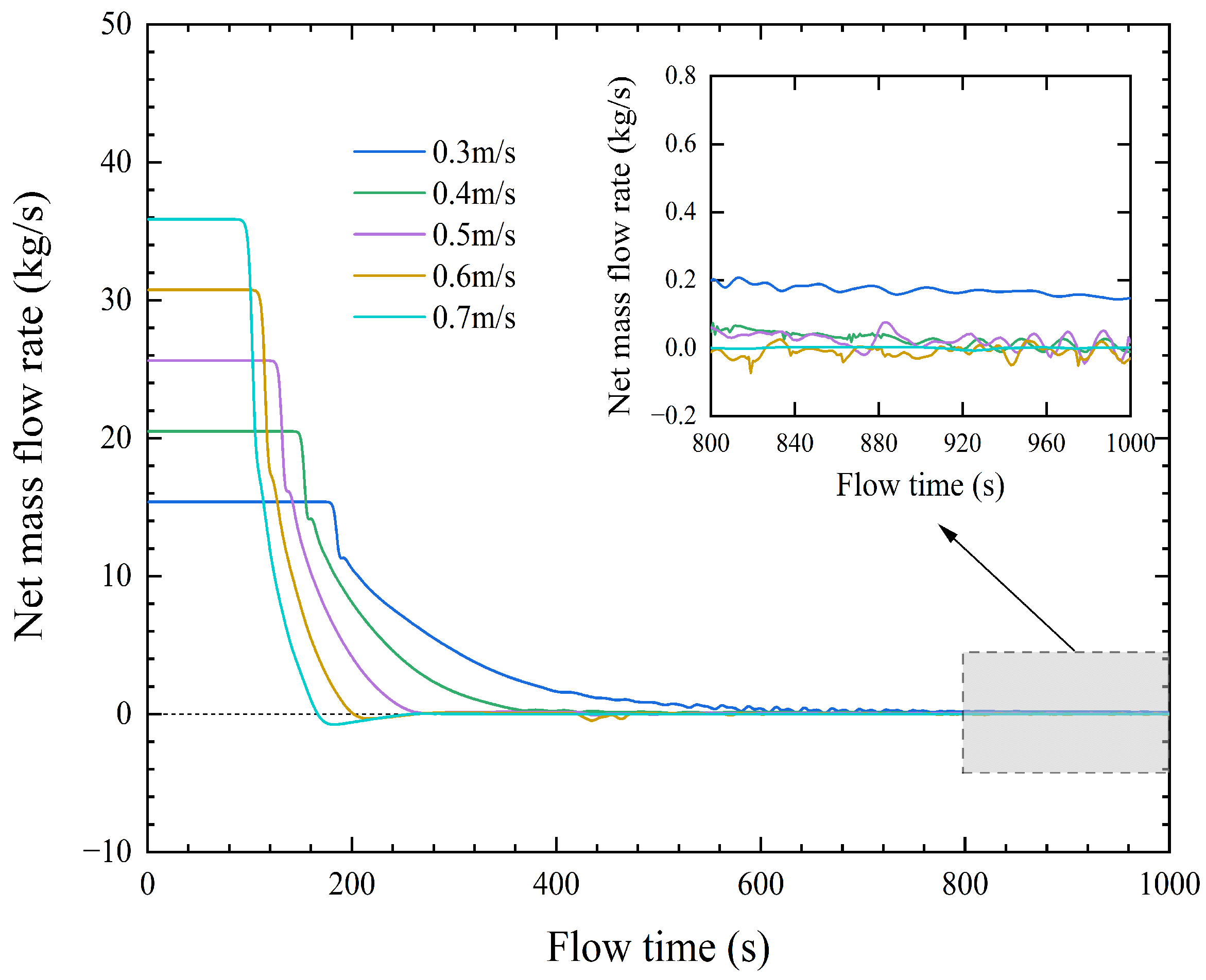
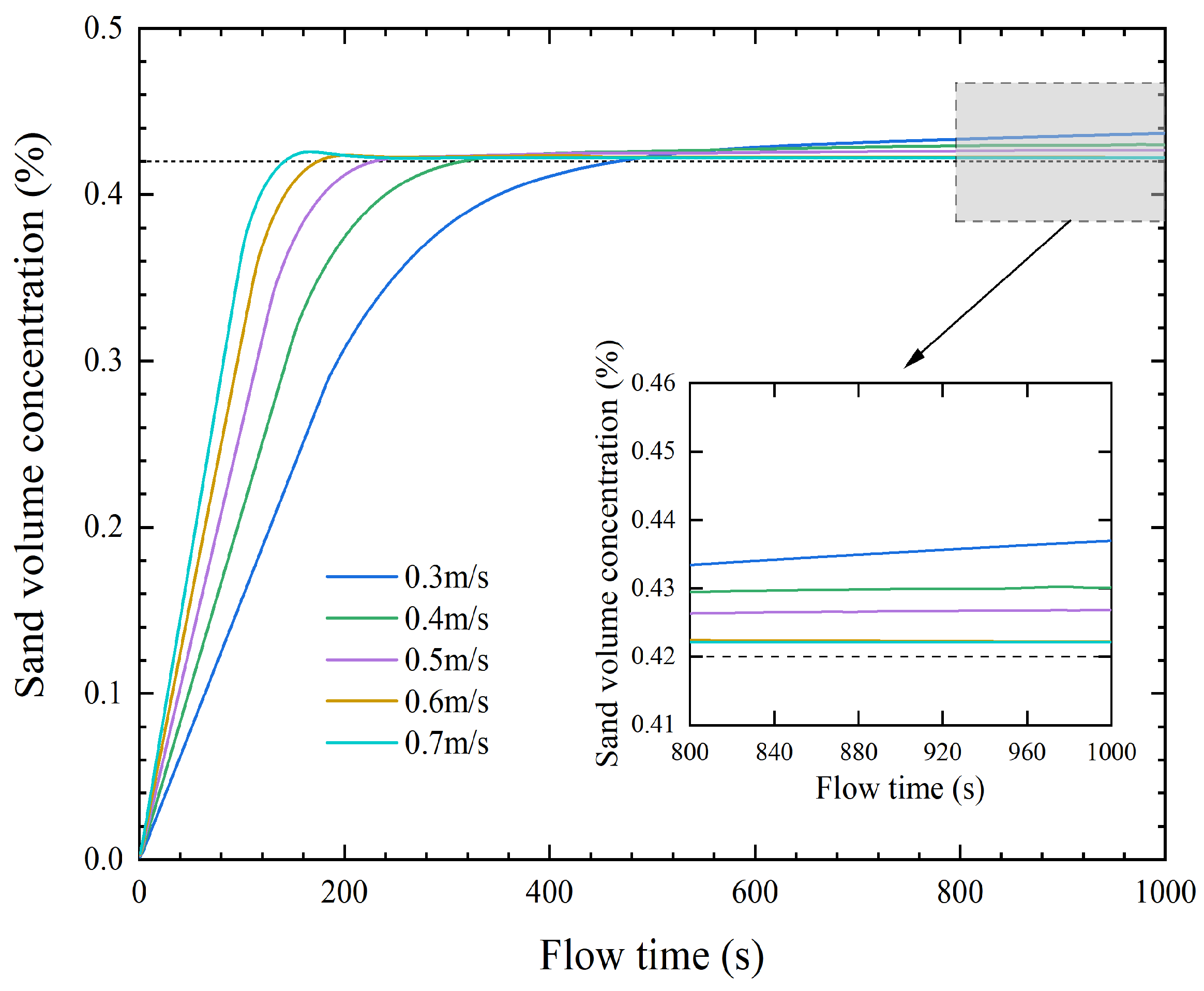
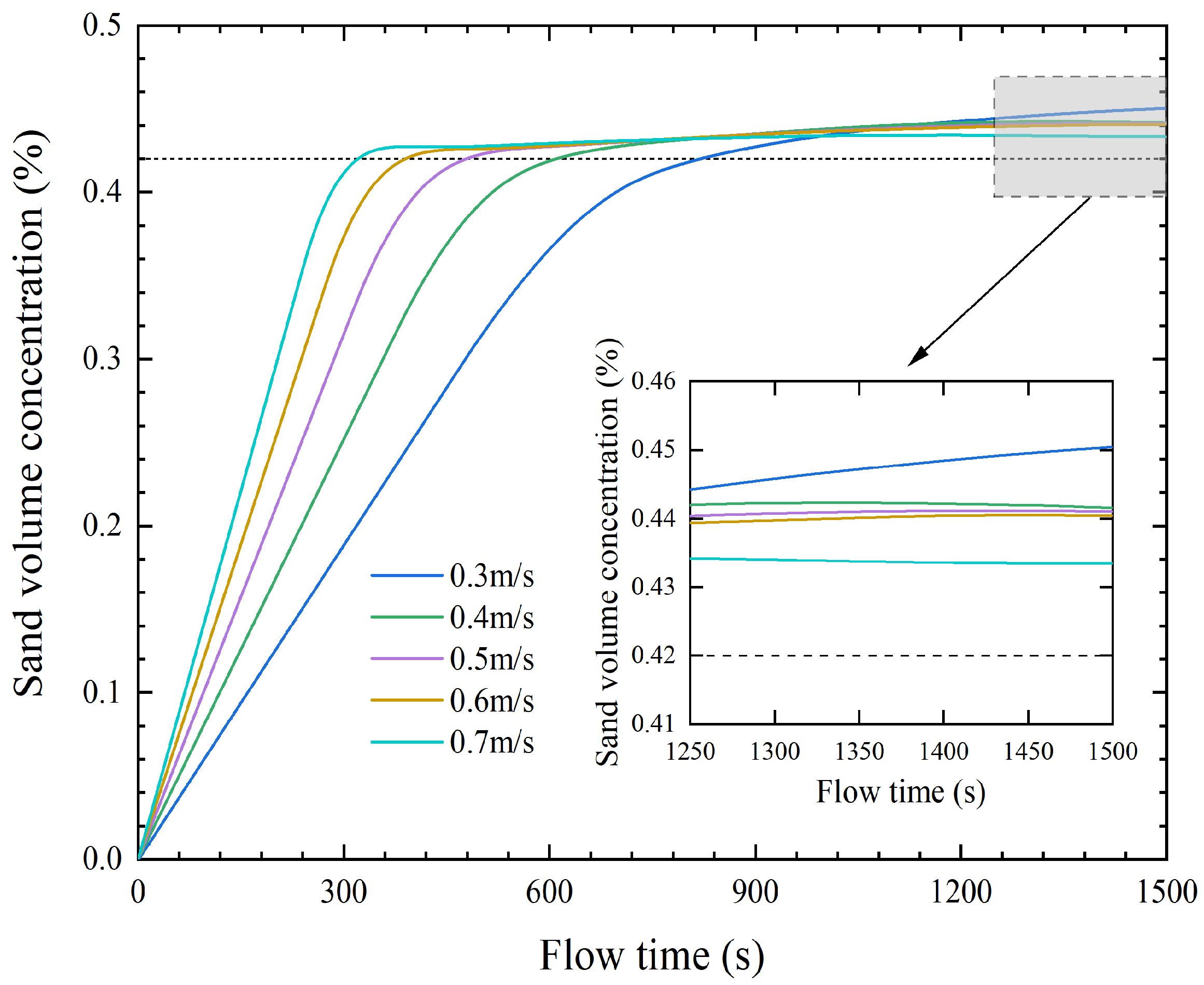
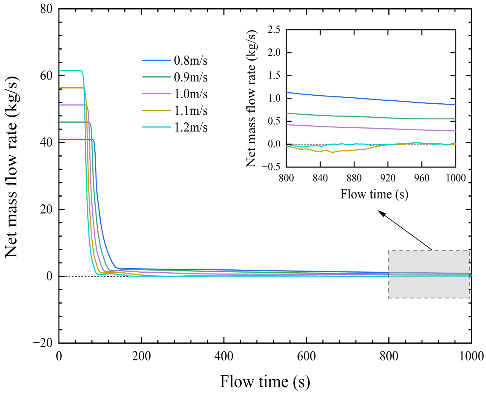
Three-dimensional numerical simulations under different inflow velocities for the horizontal pipe in Table 2 were carried out. Figure 3 and Figure 4 show the change in net mass flow rate and sand volume concentration with time under different inflow velocities. It can be seen from Figure 3 that the net mass flow rate of sand was basically stable after the flow time of 1000 s. When the inflow velocity was greater than 0.3 m/s, and the net mass flow rate was stable near 0, that is, the sand transport at the inlet was equal to that at the outlet, and the equilibrium between transport and deposition was achieved. When the inflow velocity was 0.3 m/s, the net mass flow rate was stable around a certain value but still greater than 0, which indicates that the sand increases with time under this inflow velocity, and a part of sand is deposited at the bottom of the pipe. This conclusion can also be seen in Figure 4. When the inflow velocity was 0.3 m/s, the sand volume concentration increased gradually with time. However, when the inflow velocity increased to 0.4 m/s, the sand volume concentration did not increase with time. The stable sand volume concentration was slightly larger than the initial given concentration of 0.42%, indicating that there was still slight sand deposition. The sand at the bottom of the pipe slides or rolls on the bed surface, but does not affect transportation. In summary, the critical velocity of the horizontal pipe was predicted to be 0.4 m/s by numerical simulation.

The parameters of sand used in this paper come from real data from the pipeline irrigation project of the Yellow River irrigation area. The test sand sample of the He Wuquan formula is also from the Yellow River, so this empirical formula was selected to verify the accuracy of numerical simulation. Substituting the parameters of horizontal pipe in Table 2 into the He Wuquan formula, the critical velocity was found to be as 0.43 m/s. The results from the numerical simulation are in general agreement with this, which illustrates the accuracy of the numerical simulation in predicting the critical velocity.

3.2. Effect of Simulated Pipeline Length

The length of the pipeline in the irrigation project of the Yellow River irrigation area is as long as 40 km. Affected by computer performance, the three-dimensional numerical simulation of the entire pipeline cannot be carried out. Therefore, the effect of different simulated pipeline lengths on predicting the critical velocity of the pipe was investigated. The research object was the V-inclined pipe shown in Table 2. The simulated pipeline lengths were selected to be 80 m, 150 m and 200 m, respectively, and the particle size was set to 0.02 mm.

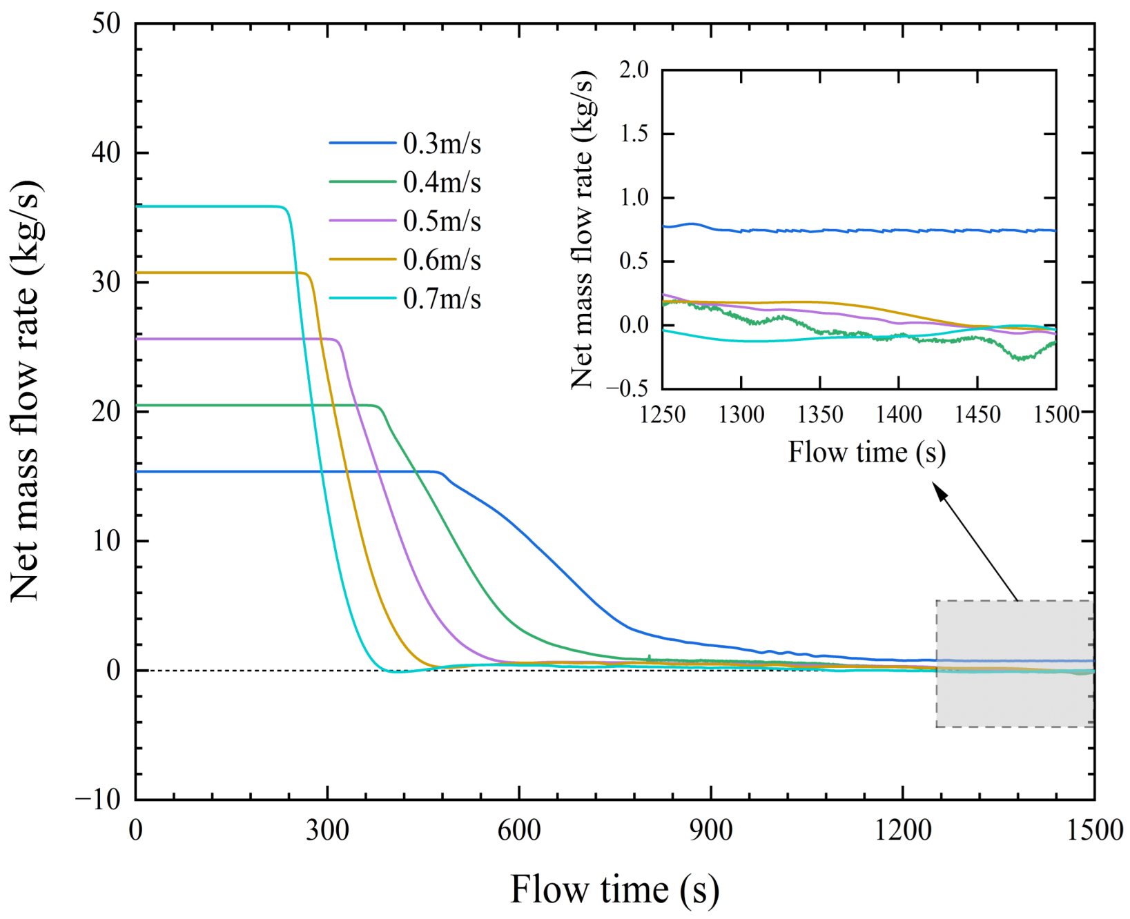
As shown in Figure 5, Figure 6 and Figure 7, there was a change in the net mass flow rate with flow time under different simulated pipeline lengths of 80 m, 150 m and 200 m, respectively. It can be seen that the net mass flow rate of sand was basically stable after 1000 s, 1200 s and 1500 s for the simulated pipeline lengths of 80 m, 150 m and 200 m, respectively. When the inflow velocity was greater than 0.3 m/s, the net mass flow rate was stable near 0, reaching equilibrium between transport and deposition. When the inflow velocity was 0.3 m/s, the net mass flow rate was stable around a certain value, but still greater than 0. This shows that the sand in the pipe keeps increasing with time.

As shown in Figure 8, Figure 9 and Figure 10, there was a change in sand volume concentration with flow time under different simulated pipeline lengths of 80 m, 150 m and 200 m, respectively. It can be seen that at the inflow velocity of 0.3 m/s, sand volume concentration had been increasing under the three simulated pipeline lengths, which is related to the fact that the net mass flow is not 0 after a certain period of flow, indicating that there is a continuous sand deposition in the V-inclined pipe. When the inflow velocity increased to 0.4 m/s, sand volume concentration no longer changed with time under the three simulated pipeline lengths. Therefore, the amount of sand deposition does not increase over time. The critical velocity of the V-inclined pipe at all three pipe lengths was 0.4 m/s.

In summary, the simulated pipeline length had almost no effect on the prediction of the critical velocity of the V-inclined pipe after a certain length. In addition, the stable sand volume concentration for different lengths at 0.4 m/s was slightly larger than the initially given value of 0.42%. Additionally, with the increase in simulated pipeline length, the sand volume concentration after stabilization was larger, which shows that simulated pipeline lengths have an effect on the amount of deposition and deposition forms.

3.3. Effect of Pipe Inclination

The effect of pipe inclination on critical velocity can be obtained by comparing Figure 3 and Figure 4 with Figure 5 and Figure 8. It can be found that under the same conditions as other parameters, the critical velocity of $\pm 2{}^{\circ }$ V-inclined pipe and horizontal pipe when transporting particles with a size of 0.02 mm is 0.4 m/s for both.

Although the $\pm 2{}^{\circ }$ pipe inclination had no obvious effect on the critical velocity, the V-inclined pipe was different from the horizontal pipe in that the pipe curvature still had an impact on the flow and sand deposition. Figure 11 shows the liquid velocity at different cross-sections when the inflow velocity was 0.4 m/s. y is the height of the pipe. It can be seen that the liquid velocity of the section conformed to the distribution characteristics of high velocity in the center of the pipe and low velocity near the pipe wall. Pipe inclination had a certain influence on the liquid velocity of the cross-sections. The liquid velocity of the horizontal pipe was symmetrical similar to that of the central axis. However, the liquid velocity of the V-shaped inclined pipe presented a nonuniform and asymmetric distribution, especially in the upward pipe. The liquid velocity near the top of the pipe was higher than that near the bottom of the pipe.

Figure 12 and Figure 13 are the sand volume concentration contours at different cross-sections of the horizontal pipe and the V-inclined pipe, respectively. It can be seen that the distribution of sand in each cross-section of the horizontal pipe was basically the same. In the V-inclined pipe, there were obvious differences between the upward and downward pipes. Sand was mainly concentrated in the upward pipe. The sand deposition was the largest at the lowest cross-section of the pipe. The low-velocity zone produced by sand deposition had an impact on the liquid velocity distribution, and the low-velocity movement of sand squeezed the main flow, thus resulting in the uniform and asymmetric distribution in Figure 11b. The fundamental reason for these phenomena is that the force on the particles in the V-inclined pipe is different from that in the horizontal pipe. The effect of gravity on the upward and downward pipes is different. In the downward pipe section, the component force of gravity is in the same direction as the flow direction, which can promote the flow of sand, while in the upward pipe section, it acts as a resistance in the opposite direction.

3.4. Effect of Particle Size

It can be seen from the empirical formula of the horizontal pipe that the relationship between the critical velocity and the particle size was complicated, and the critical velocity calculated by different formulas was very different. Therefore, the influence of different particle sizes on predicting the critical velocity of V-inclined pipe was investigated.

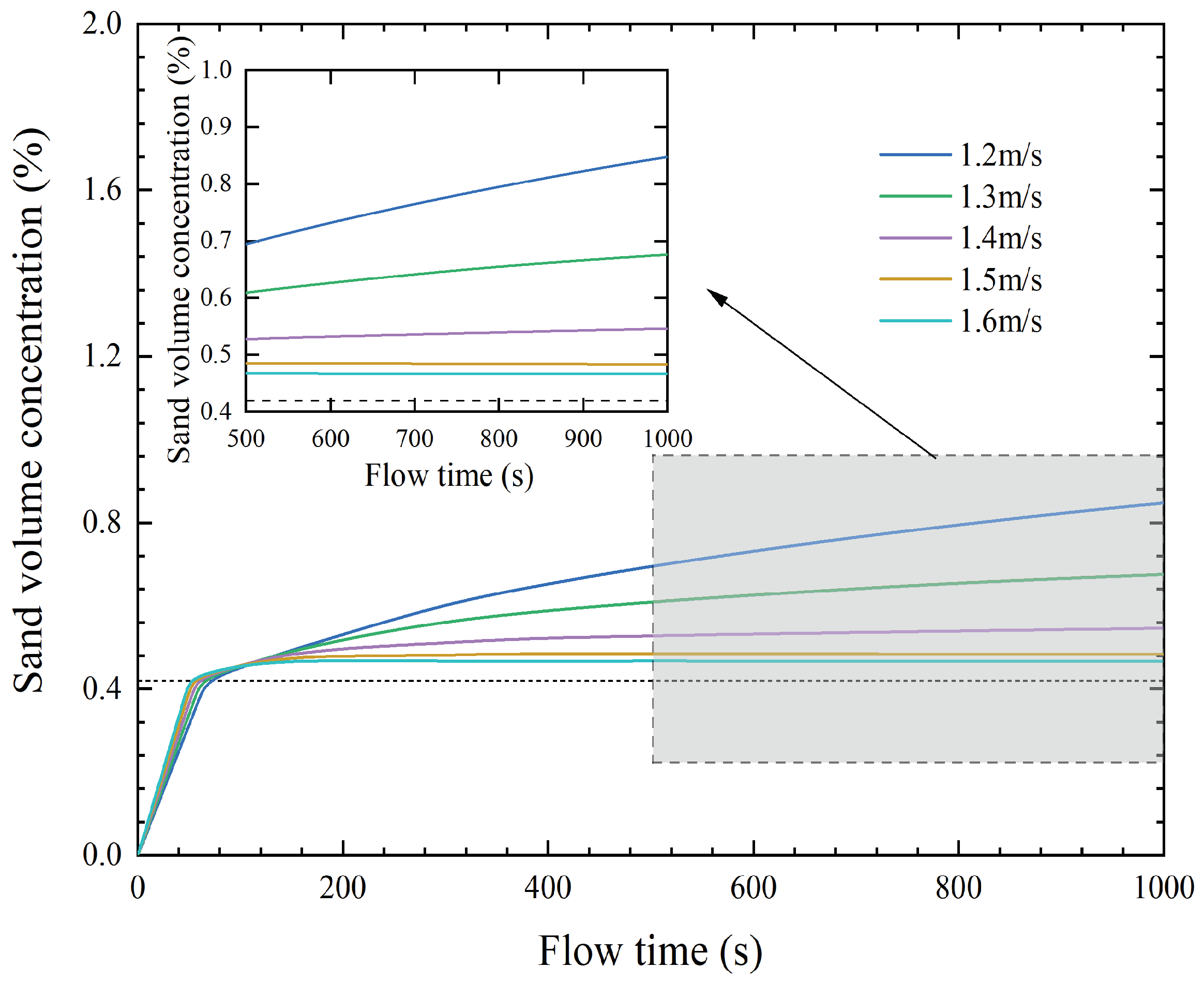
As shown in Figure 5, Figure 14 and Figure 15, there were changes in the net mass flow rate with the flow time under different particle sizes of 0.02 mm, 0.05 mm and 0.1 mm, respectively. The critical velocity was also predicted based on the conservation of the sand transport rate. It can be seen that the net mass flow rate was basically stable after the flow time of 1000 s under different particle sizes. When the flow velocity increased to 0.4 m/s, 1.1 m/s and 1.5 m/s respectively, the net mass flow rate was basically 0. At this time, sand volume concentration no longer changed with time. As shown in Figure 8, Figure 16 and Figure 17, the sand in the V-inclined pipe reached equilibrium between transport and deposition, and the amount of sand deposition did not increase with time. Therefore, the critical velocity of the pipeline under the particle sizes of 0.02 mm, 0.05 mm and 0.1 mm was 0.4 m/s, 1.1 m/s and 1.5 m/s, respectively.

As the particle size increased, the critical velocity increased accordingly, which is consistent with the force of particles in the pipe. When the particles move in the pipe, they are affected by gravity and buoyancy in the vertical direction. The larger the particle size, the easier it is to deposit, and the greater the transporting velocity is required. There was no significant difference in the critical velocity in the V-inclined pipe when the horizontal pipe transport particle size was 0.02 mm, as mentioned in Section 3.3. The critical velocity under different particle sizes was calculated using the Wasp and He Wuquan formulas, which are related to the particle size given in Table 3. The comparison between empirical formulas and numerical simulation of the V-inclined pipe is shown in

Table 4. Comparison between empirical formula and numerical simulation under different particle sizes.

Particle Size	Emprical Formula		Numerical Simulation
	Wasp	He Wuquan
0.02 mm	0.99 m/s	0.43 m/s	0.4 m/s
0.05 mm	1.16 m/s	1.10 m/s	1.1 m/s
0.1 mm	1.30 m/s	2.05 m/s	1.5 m/s

. When transporting smaller particles with particle sizes of 0.02 mm and 0.05 mm, the critical velocity calculated by the empirical formula and numerical simulation was basically the same. However, when transporting larger particles with a particle size of 0.1 mm, there was a significant difference. The reason for the difference is that, on the one hand, different empirical formulas have large differences in the prediction of critical velocity under the same particle size, and the inaccuracy of empirical formula prediction increases; on the other hand, the assumption of spherical particles is adopted in the numerical simulation, and only the drag force effect is considered between phases, which has a certain influence on the prediction of critical velocity.

4. Conclusions

Predicting critical velocity using numerical simulations can greatly reduce labor and cost. In this paper, the critical velocity of the $\pm 2{}^{\circ }$ V-inclined pipe was predicted using three-dimensional numerical simulation based on the conservation of the sand transport rate. The critical velocity predicted by the simulation of the horizontal pipe was basically consistent with the empirical formula, which verified the accuracy of the method. Numerical simulations of V-inclined pipe under different parameters were carried out, and the results show that:

(1) When the simulation length of the pipe reaches a certain value, it has no obvious effect on the prediction of the critical velocity of the V-inclined pipe. However, it will have an effect on the amount of deposition and deposition forms.

(2) Compared with the horizontal pipe, the $\pm 2{}^{\circ }$ pipe inclination has no obvious effect on the critical velocity of transporting 0.02 mm small-sized particles. In addition, the pipe inclination leads to the nonuniform and asymmetrical distribution of liquid velocity and sand deposition at different cross-sections. There are obvious differences between the upward and downward pipes. Sand is mainly concentrated in the upward pipe, and deposition is the largest at the lowest cross-section of the pipe. The effect of gravity on the particles in the downward and upward pipe is different.

(3) As the particle size increases, the critical velocity also increases. However, the effect of particle size on the critical velocity is complicated, resulting in a large difference between numerical simulation and empirical formula when transporting large-sized particles. On the one hand, the empirical formula for horizontal pipe may not be accurate in predicting the critical velocity of V-inclined pipe; on the other hand, the numerical simulation uses the assumption of spherical particles and only considers the drag effect between phases.

References

- He, W.Q.; Cai, M.K.; He, X.Y.; Zhang, C.D. Analysis and determination of critical non-silting velocity of muddy water conveyance pipelines in Yellow River irrigation districts. Paiguan Jixie Gongcheng Xuebao/J. Drain. Irrig. Mach. Eng. 2013, 31, 36–40. [Google Scholar]
- Ardiclioglu, M.; Hadi, A.M.W.; Periku, E.; Kuriqi, A. Experimental and Numerical Investigation of Bridge Configuration Effect on Hydraulic Regime. Int. J. Civ. Eng. 2022, 20, 981–991. [Google Scholar] [CrossRef]
- Daneshfaraz, R.; Aminvash, E.; Ghaderi, A.; Kuriqi, A.; Abraham, J. Three-Dimensional Investigation of Hydraulic Properties of Vertical Drop in the Presence of Step and Grid Dissipators. Symmetry 2021, 13, 895. [Google Scholar] [CrossRef]
- Daneshfaraz, R.; Norouzi, R.; Abbaszadeh, H.; Kuriqi, A.; Di Francesco, S. Influence of Sill on the Hydraulic Regime in Sluice Gates: An Experimental and Numerical Analysis. Fluids 2022, 7, 244. [Google Scholar] [CrossRef]
- Dasineh, M.; Ghaderi, A.; Bagherzadeh, M.; Ahmadi, M.; Kuriqi, A. Prediction of Hydraulic Jumps on a Triangular Bed Roughness Using Numerical Modeling and Soft Computing Methods. Mathematics 2021, 9, 3135. [Google Scholar] [CrossRef]
- Lu, Z.; Xiao, R.; Tao, R.; Li, P.; Liu, W. Influence of guide vane profile on the flow energy dissipation in a reversible pump-turbine at pump mode. J. Energy Storage 2022, 49, 104161. [Google Scholar] [CrossRef]
- Lu, Z.; Zhang, F.; Jin, F.; Xiao, R.; Tao, R. Influence of the hydrofoil trailing-edge shape on the temporal-spatial features of vortex shedding. Ocean Eng. 2022, 246, 110645. [Google Scholar] [CrossRef]
- Oudeman, P. Sand Transport and Deposition in Horizontal Multiphase Trunklines of Subsea Satellite Developments. In Offshore Technology Conference; OnePetro: New York, NY, USA, 1992. [Google Scholar]
- Bello, K.; Oyeneyin, B.; Oluyemi, G. Minimum Transport Velocity Models for Suspended Particles in Multiphase Flow Revisited. In Proceedings of the SPE Annual Technical Conference and Exhibition, Denver, CO, USA, 30 October–2 November 2011; Volume 4. [Google Scholar]
- Doron, P.; Barnea, D. Pressure Drop and Limit Deposit Velocity for solid–liquid Flow in Pipes. Chem. Eng. Sci. 1995, 50, 1595–1604. [Google Scholar] [CrossRef]
- Doan, Q.; Ali, S.M.; George, A.E.; Oguztoreli, M. Simulation of sand transport in a horizontal well. In Proceedings of the International Conference on Horizontal Well Technology, Calgary, AB, Canada, 18–20 November 1996; pp. 581–593. [Google Scholar]
- Wasp, E.; Kenny, J.; Gandhi, R. Solid liquid flow—Slurry pipeline transportation. Trans. Tech. Publ. Rockport MA 1977, 43, 101–109. [Google Scholar]
- Shook, C. Pipelining Solids: The design of short distance pipelines. Proceedings from the Symposium on Pipeline Transport of Solids; Canadian Society for Chemical Engineering: Toronto, ON, Canada, 1969. [Google Scholar]
- Kokpinar, M.; Gogus, M. Critical Flow Velocity in Slurry Transporting Horizontal Pipelines. J. Hydraul. Eng. 2001, 127, 763–771. [Google Scholar] [CrossRef]
- Azamathulla, H.M.; Ahmad, Z. Estimation of Critical Velocity for Slurry Transport through Pipeline Using Adaptive Neuro-Fuzzy Interference System and Gene-Expression Programming. J. Pipeline Syst. Eng. Pract. 2013, 4, 131–137. [Google Scholar] [CrossRef]
- Durand, R. Basic relationships of the transportation of solids in pipes-experimental research. In Proceedings of the International Association of Hydraulic Research, Minneapolis, MN, USA, 1–4 September 1953; pp. 89–103. [Google Scholar]
- Thomas, D. Transport Characteristics of Suspensions: Application of Different Rheological Models to Flocculated Suspension Data. In Progress in International Research on Thermodynamic and Transport Properties; Academic Press: Cambridge, MA, USA, 1962; pp. 704–717. [Google Scholar]
- Graf, W.; Robinson, M.; Yucel, O. Critical velocity for solid–liquid mixtures. In Proceedings of the 1st Conference on Hyd Transport of Solids in Pipes, BHRA Fluid Engineering, Cranfield, UK; 1970. [Google Scholar]
- He, W.; Wang, Y.; Zhang, Y. Experimental on Muddy Water Delivery for Irrigation in Low-pressure Pipeline System. J. Shenyang Agric. Univ. 2007, 38, 98–101. [Google Scholar]
- Jie, A.N.; Zong, Q.; Tang, H. Experimental Study on Non-depositing Critical Velocity of Muddy Water Delivery in Low-pressure Pipeline System. J. Shihezi Univ. (Natl. Sci.) 2012, 30, 83–86. [Google Scholar]
- Sajeev, S.; Mclaury, B.; Shirazi, S. Critical Velocities for Particle Transport from Experiments and CFD Simulations. Int. J. Environ. Ecol. Eng. 2017, 11, 538–542. [Google Scholar]
- Ling, J.; Skudarnov, P.V.; Lin, C.X.; Ebadian, M.A. Numerical investigation of liquid-solid slurry flows in a fully developed turbulent flow region. Int. J. Heat Fluid Flow 2003, 24, 389–398. [Google Scholar] [CrossRef]
- Kaushal, D.R.; Thinglas, T.; Tomita, Y.; Kuchii, S.; Tsukamoto, H. CFD modeling for pipeline flow of fine particles at high concentration. Int. J. Multiph. Flow 2012, 43, 85–100. [Google Scholar] [CrossRef]
- Januário, J.; Maia, C. CFD-DEM Simulation to Predict the Critical Velocity of Slurry Flows. J. Appl. Fluid Mech. 2020, 13, 161–168. [Google Scholar] [CrossRef]
- Dabirian, R.; Arabnejad Khanouki, H.; Mohan, R.S.; Shoham, O. Numerical Simulation and Modeling of Critical Sand-Deposition Velocity for Solid/Liquid Flow. SPE Prod. Oper. 2018, 33, 866–878. [Google Scholar] [CrossRef]
- Yang, Y.; Peng, H.; Wen, C. Sand Transport and Deposition Behaviour in Subsea Pipelines for Flow Assurance. Energies 2019, 12, 4070. [Google Scholar] [CrossRef]
- Al-lababidi, S.; Yan, W.; Yeung, H. Sand Transportations and Deposition Characteristics in Multiphase Flows in Pipelines. J. Energy Resour. Technol. 2012, 134, 034501. [Google Scholar] [CrossRef]
- Danielson, T. Sand Transport Modeling in Multiphase Pipelines. In Proceedings of the Offshore Technology Conference, Houston, TX, USA, 30 April–3 May 2007. [Google Scholar]
- Dabirian, R.; Mohan, R.; Shoham, O.; Kouba, G. Sand Transport in Slightly upward-inclined Multiphase Flow. J. Energy Resour. Technol. 2018, 140, 072901. [Google Scholar] [CrossRef]
- Tebowei, R.; Hossain, M.; Islam, S.Z.; Droubi, M.G.; Oluyemi, G. Investigation of sand transport in an undulated pipe using computational fluid dynamics. J. Pet. Sci. Eng. 2018, 162, 747–762. [Google Scholar] [CrossRef]
- Nossair, A.; Rodgers, P.; Goharzadeh, A. Influence of Pipeline Inclination on Hydraulic Conveying of Sand Particles. In Proceedings of the ASME International Mechanical Engineering Mechanical Engineering Congress and Exposition, Houston, TX, USA, 9–15 November 2012; Volume 7. [Google Scholar]
- Stevenson, P.; Thorpe, R.B. Towards understanding sand transport in subsea flowlines. In Proceedings of the 9th International Conference on Multiphase ’99: Cannes, Paris, France, 16–18 June 1999; pp. 583–594. [Google Scholar]
- Wang, J.; Li, Y.; Pan, L.; Lai, Z.; Jian, S. Study of the Sediment Transport Law in a Reverse-Slope Section of a Pressurized Pipeline. Water 2020, 12, 3042. [Google Scholar] [CrossRef]
- Li, M.Z.; He, Y.P.; Liu, Y.D.; Huang, C. Hydrodynamic simulation of multi-sized high concentration slurry transport in pipelines. Ocean Eng. 2018, 163, 691–705. [Google Scholar] [CrossRef]
- Parkash, O.; Kumar, A.; Sikarwar, B.S. Analytical and comparative investigation of particulate size effect on slurry flow characteristics using computational fluid dynamics. J. Therm. Eng. 2021, 7, 220–239. [Google Scholar] [CrossRef]
- Ekambara, K.; Sanders, R.S.; Nandakumar, K.; Masliyah, J.H. Hydrodynamic Simulation of Horizontal Slurry Pipeline Flow Using ANSYS-CFX. Ind. Eng. Chem. Res. 2009, 48, 8159–8171. [Google Scholar] [CrossRef]
- Alihosseini, M.; Thamsen, P.U. Analysis of sediment transport in sewer pipes using a coupled CFD-DEM model and experimental work. Urban Water J. 2019, 16, 259–268. [Google Scholar] [CrossRef]
Figure 1.
Schematic of the V-inclined pipe.
Figure 2.
Grid structure of the pipe.
Figure 3.
Net mass flow rate changes with flow time (horizontal pipe ).
Figure 4.
Sand volume concentration changes with flow time (horizontal pipe ).
Figure 5.
Net mass flow rate changes with flow time (V-inclined pipe ).
Figure 6.
Figure 7.
Figure 8.
Sand volume concentration changes with flow time (V-inclined pipe ).
Figure 9.
Figure 10.
Figure 11.
Liquid velocity at different cross-sections (inflow velocity = 0.4 m/s).
Figure 12.
Sand volume concentration contours at different cross-sections of horizontal pipe (inflow velocity = 0.4 m/s).
Figure 13.
Sand volume concentration contours at different cross-sections of V-inclined pipe (inflow velocity = 0.4 m/s).
Figure 14.
Figure 15.
Figure 16.
Figure 17.