Estimating Soil Clay Content Using an Agrogeophysical and Agrogeological Approach: A Case Study in Chania Plain, Greece

Abstract

Thorough knowledge of soil lithology and its properties are of considerable importance to agriculture. These parameters have a direct impact on water permeability and the content of the water in soil, which represent significant factors in crop yield, decisively determining the design of irrigation systems and farming processes. In the framework of this study, and considering the inevitable impacts of climate change, the rational management of water resources and the optimization of irrigation through innovative technologies become of significant importance. Thus, we propose an interdisciplinary approach based on robust techniques from the allied fields of earth (geological mapping, geophysical methods) and soil sciences (sampling, mechanical analysis) assisted by statistics and GIS techniques. Clay or the sum of clay and silt soil content is successfully determined from the normalized chargeability using induced polarization and electrical resistivity techniques. Finally, we distinguished three classes (S1, S2 and S3) considering the clay or the sum of clay and silt soil content in the study area (a) based on the dry period geophysical data and (b) using as classification criterion the spatial distribution of the geological formations.

1. Introduction

Globally, agriculture consumes most water resources since farming activities correspond to 70% of global water usage with agricultural use in some developing countries reaching as much as 95% of all uses [1]. Irrigation is inseparable from agricultural output, since the 20% of cultivated land worldwide that is irrigated is also responsible for 40% of global food production. The global trend of accelerated dryland expansion [2] and the shifting of large portions of land to a dryer climate is well documented. Especially for the Mediterranean climate change hot-spot [3], climate model projections indicate a high level of susceptibility to water stress [4], thus risking the status of irrigation resources, which are projected to become more scarce and fragile.

Available water content (AWC) is a critical concept in managing agricultural consumption, since it is a descriptor of the effective storage of water in the soil [5], typically associated with the difference in soil water potential between 33 kPa (soil field capacity) and 1500 kPa (plant permanent wilting point). In the context of water resources management, high values of AWC per unit of soil volume allow for the longer retention of rainwater and more infrequent irrigation scheduling. Thus, the pressure on rechargeable water resources (groundwater), vegetation growth and irrigation water distribution [6] decreases. On the other hand, uncertainty about AWC can lead to overirrigation and a loss of valuable water resources below the root zone, with research showing losses that can exceed 30% of irrigated water [7,8,9]. The exact determination of water retention characteristics at soil sample level typically involves expensive and time-consuming lab work [10,11] but can also be predicted using data-driven approaches [12,13], the most popular of which is arguably ROSETTA [14]. While spatial datasets of AWC do exist [15,16] and are widely used [17], scaling AWC point values in space pose a challenge due to the high spatial variability of determining soil properties (i.e., soil texture and bulk density). To overcome the challenge of spatially explicit assessment of AWC, or the soil properties that control it, various methods have been employed, for example, the use of hyperspectral imaging [18], microwave backscatter [19,20,21] and geophysical methods [22]. The latter are especially attractive because measurements can predict soil properties beyond the topsoil layer, thus providing assessments more relevant to the root zone of tree crops.

Geophysical methods, assisted by geology, have been widely used in recent decades to improve the understanding of spatial variation in soil moisture content and cation exchange capacity (CEC) of soils. One of the most promising geophysical methods is the ground-penetrating radar method (GPR), due to its high sensitivity to changes in moisture content [23]. However, this involves the challenging task of building an appropriate velocity model, which is directly associated with dielectric permittivity, used as an indicator of water saturation [24]. Electrical resistivity and electromagnetic induction methods can be combined to determine the electrical resistivity (ρ) of soils. The electrical conductivity (σ = 1/ρ) of soil depends on the temperature, the porosity, its structure, the water saturation, the dissolved salts content in the water and the clay content [25,26,27,28]. Induced polarization (IP) is a geophysical method that can be used to image two geoelectrical properties of soil: electrical conductivity (σ) and chargeability (M) [29,30]. The IP method determines the physical properties of the soil, such as hydraulic conductivity [31], since the mechanism governing IP phenomena mainly occurs in the contact between pores and soil grains. The chargeability, a quantity determined by induced polarization method, is used in environmental problems studies (i.e., pollutants detection, [32,33]) and for the identification of the clay composition in geological formations [34]. The normalized chargeability (M_n), defined as the ratio of the chargeability to the electrical resistivity, is an independent parameter of the measured soil sample electrical resistivity. M_n is proportional to the quadrature conductivity (σ), which is directly related to the polarization processes occurring between pores and soil grains [35]. Consequently, M_n is proportional to the accumulation of clay minerals in the soil.

Against this backdrop and considering the strong relation between soil characteristics and water content in designing effective and climate-proof agricultural water management systems, we propose a new approach. This is based on agrogeophysical field measurements [36] assisted by agrogeological [37,38,39,40,41,42] and pedometrical methods [43,44,45,46,47] to both qualitatively and quantitatively characterize the agricultural land of Chania Plain (Crete, Greece). Specifically, the objectives of the present work are (a) to highlight the effective use of the agrogeophysical and agrogeological methods, along with soil analyses, and to interpret their results qualitatively and quantitatively and (b) to correlate the normalized chargeability of soils with the percentage of the clay content or the sum of the clay and silt content for different geological formations and for different time periods (wet and dry). The proposed method is applied in the plain of Chania in western Crete (Greece), where advancing crop-and-tree-planting planning and agricultural water-management strategies is critical to maintaining local livelihood and avoiding desertification [48].

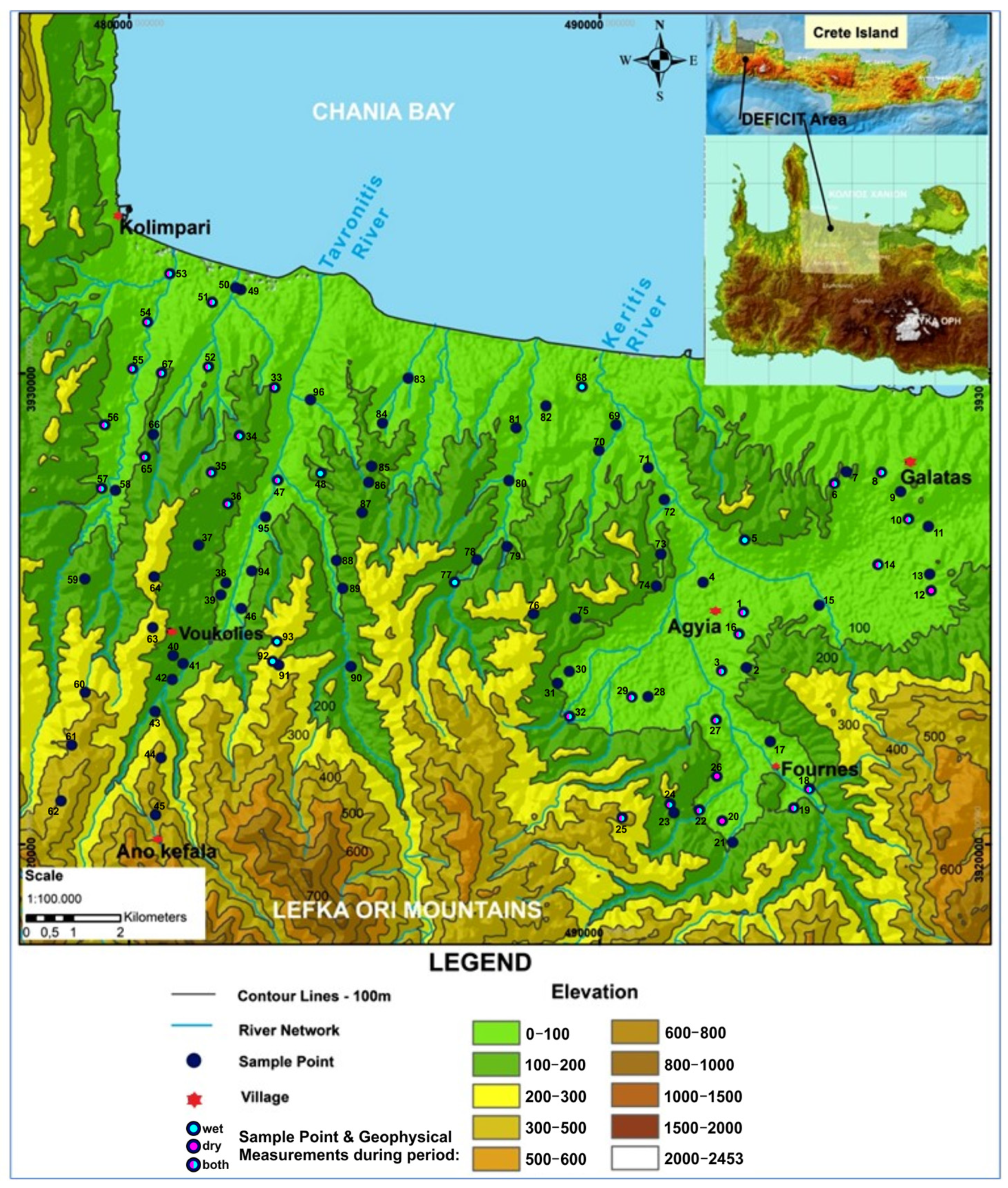
2. The Study Area

The study area, mainly cultivated with olive, avocado and citrus crops, extends in northwestern Crete covering an area of 182 km² (Figure 1). It presents a mild geomorphology with altitudes ranging from sea level, along the northern coastline, to about 700 m above sea level (masl), close to the foot of the Lefka Ori Mountains to the south, while the average altitude is 270 masl. The stream network of the study area is complex, with prevailing rivers being the northward-flowing Keritis and Tavronitis (Figure 1). From the geological point of view, this area is a tectonic basin, created under the intense tectonic influence of normal faults within the neotectonic period [49,50,51,52]. In the middle of the Agyia Plain (Figure 1), a significant group of springs exists, representing the natural discharges of the Lefka Ori Mountains’ karstic aquifers, with an average annual discharge of 80 Mm³ [49].

The geological formations of the study area are shown in Figure 2 and in Figure A2 and Figure A3 (Appendix A). The geological structure of the study area corresponds to a tectonic pile of nappes, successively superimposed on each other, within the Alpine orogeny, in a compression regime, closely associated with the tectonic plates’ convergence [50,53,54]. They include the lower nappes of the Plattenkalk unit (Pk), Tripalion unit (Trip), phyllite–quartzite unit (Ph) and the upper nappes of Tripolis and Pindos as well [50,52,55].

In Miocene times, the southward migration of the convergence’s limit between the Eurasian and African plates affected the extension in Crete region. This impacted the uplifting and the extensional exhumation of the lower tectonic nappes (carbonate rocks of the Lefka Ori tectonic window) [50,51,52]. During this evolution, major fault zones enabled large-scale uplift, resulting in normal faults [51]. Such fault zones, mainly trending NNW–SSE and WSW–ENE, are nowadays the borders of the Lefka Ori Mountains and the related tectonic basins. The largest of these basins is the Agyia-Galatas basin (Figure 1), where the Neogene and Quaternary sediments from the Miocene to now were deposited. These are the geological deposits of the Miocene (Ms, Me), Pliocene (Plm), Pleistocene (dl) and Holocene (al), mainly consisting of marls, sandstones, marly limestones, conglomerates, clays, sands, gravels and pebbles.

The map in Figure 2 provides the necessary information, especially regarding the exact demarcation and lithology of the geological formations covering the study area. The lithological differentiation of the geological formations is undoubtedly related to the upper soil composition (0–3 m below the surface), which further affects the crop growth. The upper soil layers are constantly enriched with the products of erosion, transferred from surface water flow through the hydrographic network of the area. The water flow of the streams erodes the geological formation passing through. So, the composition of the upper soil layers varies according to the upstream geological formation.

According to the Koppen climate classification, the area of West Crete is classified in the Cs subgroup, so the climate is characterized as a wet, subtropical, Mediterranean climate, with a rainy winter and six months of nearly dry summer ([50] and references therein). Crete has a remarkable annual overall potential of groundwater (2.2 × 10⁹ m³) and surface water resources (1.2 × 10⁹ m³) due to the high average annual precipitation (7.7 × 10⁹ m³) and the existence of the mountain ranges mainly consisting of permeable carbonate bedrock [56]. The temperate climatic conditions contribute, among other things, to the agricultural and rural development of the investigated area, as well as for the rest of Crete. Agriculture is one of the main pillars of Crete’s economy, and its potential for further development is based on (a) the improvement of the competitiveness of traditional dynamic crops, (b) the introduction of new technologies and (c) the enhancement and promotion of the agricultural production [57].

Unfortunately, despite the substantial volume of water resources, its insufficiency for further agricultural development is an unpleasant reality. This is directly related to the substantial imbalance between the uneven distribution of water resources availability (i.e., rainfall only in winter–spring periods) and demand (significantly increased during the dry season) [57]. Further development of Crete’s agricultural economy under the pressure of increased demand and climate change [58,59] can only take place under strategic adaptation [60] in all three types of water footprints: green (rainwater taken by plants), blue (surface and groundwater used by irrigation) and gray (freshwater required to assimilate pollutants) [1]. To meet long-term future water demands, four main water resources planning and management schemes have been implemented according to European directives [57]. The first water resources planning, and management scheme concerns the wider area of the present study, aiming to supply fresh water for 300,000 inhabitants and tourists and to irrigate 220 km² of land. The project is approximately 70% complete and is now currently in operation [61,62].

3. Methodology

3.1. Geological Mapping and Soil Sampling

The terrain model (Figure 1) in this work is from NASA Shuttle Radar Topography Mission Global 1 arc second (~30 m) V003 (https://earthexplorer.usgs.gov/), while the geological map, shown later, was compiled from [50]. In addition, soil sampling in arable fields took place in 96 sites of the study area located in western Crete (the region of Chania), in both wet and dry periods. Furthermore, a single soil sample from a depth of 0.1 up to 0.3–0.4 m was acquired at each site, next to or very close to geophysical sections, and was considered a representative sample for each studied site. Soil samples were taken aiming to (a) characterize the geological nature of the arable soils (Figure A2, Appendix A), (b) define the mechanical composition, (c) support and further interpret the results of the geophysical survey and (d) contribute to the interpretation of the soils hydro-lithological behavior closely related to their texture and physical properties. ArcGIS Pro (https://www.esri.com/en-us/arcgis/products/arcgis-pro/overview, accessed on 1 June 2022) was used to visualize the spatial data, shown in this work.

3.2. Geophysical Methods

A geophysical survey was conducted at 38 sites within Chania Plain (Figure 1), based on the geological characterization of the arable soils. We applied electrical resistivity tomography (ERT) and induced polarization (IP) geophysical methods as most appropriate according to the nature and texture of the soils covering the study area. Specifically, the geophysical survey took place at 30 sites twice, i.e., in the dry (June–August of 2020 and 2021) and wet (November–February of 2020 and 2021) periods, and at eight sites only once in either the wet or dry period. The length of each geoelectrical section was 3.9 m, and we used forty (40) electrodes spaced every 0.1 m. The gradient electrode array [63] was applied, providing 0.83 m maximum depth of investigation (Figure 3). Since ERT and IP methods map the electrical resistivity and the chargeability in two dimensions, we acquired soil samples along the geoelectrical line, as near as possible to the center of the line aiming to provide information for a single subsurface point (usually from 0.1–0.3 m depth).

An example of the collected data from two sites (#6 and #29) is shown in

Table A1. Collected data from sites #6 and #29.

Parameter	Site 6		Site 29
Position (X,Y) (HGRS87) 1	494983, 3927674		490678, 3923134
Local area	Galatas		Vatolakos
Soil sampling date	17 December 2019		14 February 2020
Soil sample name	deficit 6		deficit 29
Clay (%)	21.12		11.44
Silt (%)	41.28		20.56
Sand (%)	37.60		68
EC (dS/m)	0.34		1.07
EC sterr. (dS/m)	0.03		0.01
pH	8.33		5.27
pH sterr.	0.09		0.07
P Olsen (ppm)	14.33		100.06
P Olsen sterr. (ppm)	1.90		3.87
TKN (mg/kg)	1026.67		2298.33
TKN sterr. (mg/kg)	222.59		30.87
Ca / Mg (mg/kg)	4142/4.98		713.30/5.01
Ca / Mg sterr. (mg/kg)	334.0/0.04		22.30/0.01
Texture	Lo		SaLo
Crop	Grapes		Avocado
Geology	Marly sandstone series		Alluvial deposits
Geological description	Brownish-yellow loose marly gravel		Lose soil consisting of clay mixed with gravel of mostly fillites–quartzites composition
Geological age	Middle-Upper Miocene		Quaternary
Period of geophysical measurements (wet|dry)	November 2020	August 2020	November 2020	August 2020
Resistivity section RMS (%) (wet|dry)	1.53	8.28	3.49	14.86
Mean resistivity (Ohm.mOhm.m) (wet|dry)	28.7	666.1	319.0	2230.6
Median resistivity (Ohm.mOhm.m) (wet|dry)	29.2	236.2	239.2	1628.4
Resistivity standard deviation (wet|dry)	3.7	1160.8	265.4	1893.7
Norm. Chargeability section RMS (%) (wet|dry)	2.49	11.44	4.51	9.21
Mean Norm. Chargeability (mS/m) (wet|dry)	4.86 × 10−2	4.50 × 10−3	2.13 × 10−2	1.25 × 10−3
Median Norm. Chargeability (mS/m) (wet|dry)	2.94 × 10−2	2.12 × 10−3	1.94 × 10−2	4.38 × 10−4
Norm. Chargeability standard deviation (wet|dry)	6.04 × 10−2	7.79 × 10−3	1.07 × 10−2	1.97 × 10−3
Regression weight (wet|dry)	1.91	1.76	2.30	1.80

Note: ¹ Hellenic Geodetic Reference System 1987.

(Appendix A) during the dry and wet periods.

3.3. Soil Analyses

Soil samples (n = 96) were air-dried at 45 °C for about 48 h; small rocks and root debris were then manually removed, and samples were sieved in a 2 mm sieve. The fraction under 2 mm was collected and ground to homogeneity using a porcelain mortar. Soil texture analysis was performed by dispersing samples of known dry weight in a column of water and measuring the density of the suspension at predetermined intervals afterwards [43,44]. Precisely 50 g of the dried and sieved soil was placed in a tube along with 100 mL of 0.1 N sodium hexametaphosphate, and the mixture was stirred for 5 min. The mixture was then transferred to a 1250 mL cylinder, which was filled with distilled water to 1130 mL. Density was measured using a hydrometer after 40 s, 2 h and 4 h to account for settling sand, silt and clay fractions, respectively. During the procedure, the temperature was measured to correct for density changes.

Saturated extract electrical conductivity ${\mathrm{EC}}_{\mathrm{se}}$ [dS m⁻¹] was estimated from a 1:2 soil solution in distilled water (${\mathrm{EC}}_{1:2}$ [dS m⁻¹]) after [64]:

$${\mathrm{EC}}_{\mathrm{se}}=0.94\left[14-0.13\mathrm{C}\right]{ \mathrm{EC}}_{1:2}$$

(1)

where $\mathrm{C}$ is the percentage of clay in the sample. ${\mathrm{EC}}_{1:2}$ was determined using HQ40D Multi (HACH). Available water content (AWC) [%] was estimated using the R implementation of the ROSETTA model [65,66] in the 33 kPa to 1500 kPa interval using the sand, silt and clay soil fractions as input. The unpaired Wilcoxon test was used to compare soil sample groups for significant differences in soil texture, EC and AWC.

3.4. Sample Classification

According to the surface geological structure and the expected inherent resistivity [67], soil samples were classified in three classes (S1, S2 and S3), as shown in

Table 1. Sample classification according to surface geological structure. Geology symbols drawn from Figure 2. Ranges of resistivity values based on [67].

Sample Class	Geology Symbol	Resistivity (ohm.m)	Underlying Geology
S1	Me, Ph	103–2 × 106	Loose sediments consisting of red quartzitic–phylitic conglomerate, breccia and phyllite–quartzite unit
S2	al	10–103	Alluvial deposits consisted of loose clay materials, sand, gravel and pebbles
S3	Plm	1–102	White yellow and well-bedded marls

. Class spatial distribution is shown in Figure 2. Other classification scenarios were also considered based on other geomorphological characteristics of the sampled locations. Nevertheless, the classification based on geological features proved the most robust for the subsequent analysis of the geophysical measurements. The proposed classification distinguishes between quartzitic–phylitic (S1) and alluvial parent material (S2), which have distinct resistivity value ranges, and marls (S3), the resistivity value range of which largely overlaps that of S2.

3.5. Statistical Analysis

To compare the properties of ERT and IP geophysical methods with the soil properties deduced from sampling, we calculated (a) the average value, (b) the median value and (c) the standard deviation of resistivity and normalized chargeability within an effective length (1–3 m) and depth (0.1–0.3 m) of the corresponding section (see black frames in Figure 3), as well as (d) the RMS error of data inversion (Table A1, Appendix A). The RMS error is an expression of the section reliability (difference between observed and calculated resistivity/chargeability), and it is based on the measured noise level. Namely, from each geophysical section (resistivity or normalized chargeability), we selected a relatively narrow window (see black rectangle in Figure 3), and we evaluated the mean and median values of resistivity and normalized chargeability. These values are considered representative for the entire studied site.

Furthermore, aiming to correlate the results of the geophysical survey with the mechanical composition of soils, we produced two types of cross-plots related to (a) the resistivity versus normalized chargeability and (b) the normalized chargeability versus the clay or the sum of the clay and silt soil content. Concerning the cross-plots (log–log diagrams) of resistivity versus the normalized chargeability, we categorized the data into three depth zones: the 1st zone ranges between the surface and 0.08 m, the 2nd zone from 0.08 m to 0.28 m and the 3rd zone from 0.28 m to 0.83 m. For the cross-plots of the normalized chargeability and the clay or the sum of clay and silt soil content, we selected to present the dry period data within the effective data window (length, 1–3 m, and depth, 0.1–0.3 m) of the corresponding section (Figure 3). This is because the effect of water content on electrical conductivity measurements during the wet season tends to mask the influence of the soil texture [68]. Linear regression was performed on the data mentioned above using both ordinary (OLS, [69]) and weighted least squares (WLS, [70]). The linear formula, extracted from the regression, is:

log₁₀(M_n) = a·log₁₀(%cnt) + log₁₀(b)

(2)

where %cnt is the percent of clay content or the sum of clay and silt content, while a and b are the slope and the intercept of the line, respectively. The weights (W) in WLS were calculated using the normalized-to-the-mean value (mnv) standard deviation (std) of the data within the effective window of the section, according to the formula:

W = 2 + log₁₀(mnv/std)

(3)

In order to increase the goodness of fit of the regression models, principal component analysis (PCA) [71] was applied using as input data the log₁₀(%clay) and log₁₀(M_n) values for the dry period data set (33 sites). Four (4) points were removed as outliers, while the remaining 29 sites were distributed to two classes, providing high coefficients of determination (R²) in regression. However, there was a difficulty in attributing any new measurement (M_n) points to the classes produced by PCA, because we could not establish a generalized model of the classes considering the agrogeological and pedological data. Thus, we decided to base the data classification on the spatial distribution of the geological formations in the study area, and we finally classified the dry period data (33 sites) in three new classes (S1, S2 and S3), as shown later in the text.

4. Results and Discussion

4.1. Geophysical Properties of the Soils and Statistical Processing

High values of the normalized chargeability are observed in soils with high clay content [72]. From the combination of a geoelectric section (electrical resistivity) with the section of chargeability, it is possible to depict zones rich in clay minerals, as well as to evaluate the volumetric water content in the soil pores’ space [73]. Under the assumptions that the volumetric water content of soils is reduced during the dry period and that soil bulk density variation (from 1 to 1.6 g/cm³ for heavy to coarse soil texture, respectively) is neglected, soil clay content is the major parameter that affects the values of the normalized chargeability. This implies that no great variations in water content and bulk density are anticipated at the sites of the same class (same geological setting), and thus, the normalized chargeability is mostly affected by the clay content. Furthermore, it has been observed that high normalized chargeability values correspond to sediments with high clay content, while soils with uniform size of sand and gravel particles tend to provide lower values of resistivity and normalized chargeability in geoelectrical measurements. In addition, resistivity values of 10 to 100 ohm.m and normalized chargeability (M_n) greater than 0.07 mS/m correspond to soils with sufficient clay content, while M_n less than 0.07 mS/m correspond to reduced or non-existent clay content [74,75]. Induced polarization measurements in the frequency domain (SIP) can provide information on soil structure, such as the range of grain size distribution [76].

Figure 4 and Figure 5 display the resistivity and normalized chargeability data from the sites #22 and #14 in log₁₀–log₁₀ diagrams. At site #22 (Figure 4), the electrical resistivity (ρ) values are, in general, smaller during the wet period (blue color points) compared to those of the dry one (red color points). This is because of the increased percentage of water content. In addition, almost no measurements meet the criterion of increased clay content (i.e., ρ < 100 ohm.m or log₁₀(ρ) < 2 and M_n > 0.07 mS/m or log10(M_n) > −1.155) at site #22 (see green frame in Figure 4). Concerning the data of the wet period, log₁₀(ρ) and log10(M_n) from all three zones are linearly correlated (blue line in Figure 4). On the other hand, the data of the dry period are more scattered compared to those of the wet period, thus a distinct separation between the 1^st, 2^nd and 3^rd zones (crosses, circles and stars, respectively) is present. Furthermore, there is a linear correlation between the log₁₀(ρ) and log10(M_n) data of each depth zone for the dry period data. Blue and red lines in Figure 4 indicate the linear regression of wet and dry period data (all zones), respectively, while the black line shows the linear regression considering data from both periods.

At site #14 (Figure 5), the electrical resistivity (ρ) values are, in general, smaller during the wet period (blue color points) compared to those of the dry one (red color points), due to the increased percentage of water content. At this site, almost 50% of the measurements meet the above-mentioned criterion of increased clay content (ρ < 100 ohm.m or log₁₀(ρ) < 2 and M_n > 0.07 mS/m or log10(M_n)> −1.155—green frame in Figure 5). For the wet period data, there is a linear correlation between log₁₀(ρ) and log10(M_n) from all three zones (blue line in Figure 5). On the other hand, the data of the dry period are more scattered, and the different depth zones are not well distinct. The dispersion of datapoints in Figure 4 and Figure 5 is somehow regularized in this study by taking into consideration the mean (or median) value from depths of 0.1 to 0.3 m along the distance of 1 to 3 m from each geophysical section.

The evaluated mean (or median) value of normalized chargeability is related to the clay or the sum of clay and silt content of the sample and together consist of one point in the charts of Figure 6, Figure 7 and Figure 8. Specifically, the dry period data set (33 sites) was divided into three classes (S1, S2 and S3) based on the geological classification of the surveyed positions, while data from two control sites (#19 from class S1 and #54 from class S2) were excluded from the regression to be used for regression evaluation. The data classification was essential, both because the regression of the total dataset was a poor fit (R² = 0.2658 and 0.2543 for OLS and WLS in Figure 6a,b, and

Table 2. Regression parameters and evaluation of the clay content at control sites #19 and #54, using the data from all sites and from sites distributed in classes S1 and S2 deduced from the geological classification of the surveyed positions.

	All Sites (Dry Period) (Apart from #19 and #54)				Class S1 Sites (Dry Period) (Apart from #19)		Class S2 Sites (Dry Period) (Apart from #54)
Parameters	OLS		WLS		OLS	WLS	OLS	WLS
a	2.2756		1.8909		2.5837	2.8014	3.3531	3.2618
log10(b)	−5.2798		−4.7249		−6.0734	−6.3828	−6.4873	−6.3638
b	5.25 × 10−6		1.88 × 10−5		8.45 × 10−7	4.14 × 10−7	3.26 × 10−7	4.33 × 10−7
R2	0.2658		0.2543		0.6241	0.6181	0.4587	0.4581
variance(a)	0.5108		0.5188		0.6701	0.6808	1.3270	1.3284
variance(log(b))	0.9027		0.9168		1.2074	1.2266	2.0489	2.0508
Control site #	19	54	19	54	19	19	54	54
Measured mean Mn (mS/m)	1.029 × 10−3	4.330 × 10−2	1.029 × 10−3	4.330 × 10−2	1.029 × 10−3	1.029 × 10−3	4.330 × 10−2	4.330 × 10−2
Measured clay (%)	17.44	26.72	17.44	26.72	17.44	17.44	26.72	26.72
Lower limit of clay content (%)	6.87	31.55	5.29	32.18	10.19	10.88	20.37	20.31
Evaluated mean clay content (%)	10.17	52.60	8.30	59.94	15.64	16.29	33.73	34.12
Upper limit of clay content (%)	16.09	95.70	14.31	>100	25.85	26.00	61.43	63.38

) and because the estimated mean value of the clay content for the regression evaluation sites was unacceptable (Table 2). Specifically, the red dots in Figure 6a,b correspond to the %clay vs M_n data from the 33 investigated sites. The geophysical survey was conducted during the dry period (June–August). The slanted thick solid and dashed lines, passing from the center of the data, correspond to the best-fitted lines from the OLS and WLS regression, respectively. The slanted thin solid and dashed lines, passing from the outer part of the data, correspond to the data limits, which are drawn based on ±1/4 of the regression standard deviation. Figure 6a,b shows the evaluation of the clay content with its corresponding bounds (vertical solid and dashed lines) from the M_n value measured at control sites #19 and #54, respectively. A total of 10.17% and 52.60% were the estimated mean values of the clay content for site #19 and site #54, respectively, using OLS regression (Table 1), which are far from the corresponding measured mean values (17.44% and 26.72%, respectively). The dispersion of datapoints in Figure 6 is regularized by introducing the soil class into consideration. Thus, as indicated by the regression results, the dispersion of data is considerably reduced in classes S1 and S2, compared to the entire population of data.

Figure 7a,b shows the corresponding estimated mean values of clay content for site #19 and site #54, after the division of the data into three classes (S1, S2 and S3) based on the geological classification of the surveyed sites. There is an improved correlation of M_n values with the percentile clay content for S1 and S2 classes compared to the corresponding correlation using the complete dataset. The same improvement does not apply for class S3 (Pliocene marls). The evaluated mean clay contents at site #19 using OLS and WLS regression on S1 class data are considered acceptable (Table 2). The relative errors (100 ∗ (measured clay − evaluated mean clay)/measured clay) in that case are 10.3% and 6.6% for OLS and WLS, respectively. Similarly, the relative errors for site #54 are 26.3% and 27.7% for OLS and WLS, respectively. The corresponding relative errors using the median values of clay content for site #19 were 13.8% and 15.1% for OLS and WLS, respectively, while, for site #54, the estimations are almost twice the measured values for both OLS and WLS. The corresponding linear regression for S3 subset is shown in Figure 7c. No clay content evaluation was performed due to the poor fit of class S3 data.

Figure 8a,b shows the corresponding estimated mean values of the sum of clay and silt content for site #19 and site #54, after dividing the data into three classes based on the geological classification of the surveyed positions. There was a small improvement in the correlation of M_n values with the percentile of clay and silt sum for classes S1 and S2, compared to the complete dataset’s corresponding correlation. The evaluated clay contents at site #19 using OLS and WLS regression on S1 class data are both acceptable (

Table 3. Regression parameters and evaluation of the sum of clay and silt content at control sites #19 and #54, using the data from all sites and from sites distributed in classes S1 and S2 deduced from the geological classification of the surveyed positions.

	All Sites (Dry Period) (Apart from #19 and #54)				Class S1 Sites (Dry Period) (Apart from #19)		Class S2 sites (Dry Period) (Apart from #54)
Parameters	OLS		WLS		OLS	WLS	OLS	WLS
a	3.6491		3.5606		2.7730	3.0200	3.7427	3.5385
log10(b)	−8.2898		−8.1050		−7.0375	−7.4469	−8.4434	−8.1086
b	5.13 × 10−9		7.85 × 10−9		9.17 × 10−8	3.57 × 10−8	3.60 × 10−9	7.79 × 10−9
R2	0.3131		0.3103		0.3833	0.3791	0.3858	0.3847
variance(a)	1.0434		1.0476		2.0616	2.0756	2.2299	2.2341
variance(log(b))	2.8439		2.8555		5.2412	5.2768	5.9460	5.9572
Control site #	19	54	19	54	19	19	54	54
Measured mean Mn (mS/m)	1.029 × 10−3	4.330 × 10−2	1.029 × 10−3	4.330 × 10−2	1.029 × 10−3	1.029 × 10−3	4.330 × 10−2	4.330 × 10−2
Measured clay + silt (%)	32.00	66.72	32.00	66.72	32.00	32.00	66.72	66.72
Lower limit of clay + silt content (%)	17.78	46.34	16.99	45.26	12.89	14.10	37.32	37.00
Evaluated mean clay + silt content (%)	28.38	79.09	27.37	78.23	28.87	29.96	77.92	80.58
Upper limit of clay + silt content (%)	48.60	>100	47.47	>100	82.18	78.06	>100	>100

). The relative errors, in that case, are 9.8% and 6.4% for OLS and WLS, respectively. On the other hand, the relative errors for site #54 are 16.8% and 20.8.3% for OLS and WLS, respectively. The corresponding relative errors using the median values of clay content for site #19 were 8.7% and 10.2% for OLS and WLS, respectively, while for sites #54, 47.3% and 49.1% for OLS and WLS, respectively. The corresponding linear regression for the S3 subset is shown in Figure 8c. No clay content evaluation was performed due to the poor fit of the class S3 data.

In summary, considering the cross-plot of mean normalized chargeability versus the clay soil content values (Figure 7), we concluded that the correlation of the above-mentioned parameters was not entirely clear. Since, with PCA analysis we were unable to distribute a new measured position to the extracted-from-PCA-analysis classes, we decided to apply the geological classification of the data, and we distinguished three classes (S1, S2 and S3). This classification was essential because (a) the regression of the total dataset presents a poor fit (R² = 0.2648 and 0.2543 for OLS and WLS, respectively, Figure 6a) and because (b) the results concerning the mean value of clay content from the regression evaluation sites (#19 for class S1 and #54 for class S2) were poor (see the measured and evaluated clay content from the control sites on Table 2). Considering the classification based on the geology of the study area, classes S1 and S2 present an improvement in the goodness of fit, while the S3 class does not. The S3 class related to the Pliocene marls will be the issue of future research. This is because we believe that a denser network of geophysical measurements on Pliocene marls, distributed throughout the whole year, is required to check the efficient application of the normalized chargeability for clay content evaluation.

The water content and the content of clay minerals, as well as the bulk density of the soil (through its effective porosity), affect the electrical conductivity and the chargeability of the soil. The collection of geoelectric measurements over time for different humidity conditions allows the estimation of soil properties, such as the electrical conductivity of the solid, liquid and gas phases. During the wet season, the effect of water content on electrical conductivity measurements tends to mask the influence of the other factors. In contrast, measurements under dry conditions are more favorable for estimating the porosity and the soil texture. This work shows that clay or the sum of clay and silt soil content within the investigated area can be reasonably estimated from the measurements of the normalized chargeability using IP and resistivity measurements under dry conditions. However, classification analysis seems to be essential for the improvement of the correlation of the above-mentioned parameters. In that case, the examined sites must be firstly distributed to the classes considering the spatial distribution and the nature of the geological formations. Thus, it is possible to reasonably estimate the clay, or the sum of clay and silt soil content, based on the normalized chargeability values, except Pliocene marls, which will be investigated in more detail in the future.

4.2. Soil Analysis

Overall, the three classes show minor significant differences with respect to their constituents (Figure 9), with clay content (Figure 9c) differences standing out only between classes S2 and S3 (mean values of 18.6 and 28.8%, respectively). Classes S1 and S2 have no significant differences with respect to sand (Figure 9a) and clay (Figure 9c) content but show significant differences with respect to silt (Figure 9b) content (mean values of 17.1 and 27.0%, respectively). Based on their constituents, and according to the classification triangle defined by the FAO Soil Map of Europe [77], the soils belong mainly to the medium texture (see Figure A1 in Appendix A). This similarity, as well as the similarity of S1 and S2 with respect to clay content, highlights the importance of the classification of the sampling area based on other features, such as geology. Furthermore, as shown in Figure 10a, the three classes present no significant differences in terms of electrical conductivity, which would otherwise interfere with geophysical measurements. Finally, classes S1 and S2 show significant differences with respect to AWC, with mean values of 14.1 and 15.6%, respectively (Figure 10b). This difference can be attributed to the significant difference in the amount of silt in these classes (Figure 9b). On the other hand, the AWC of class S3 shows no significant differences from that of classes S1 and S2. While a mean difference of 1.5% in terms of AWC between classes S1 and S2 seems small, one should also consider the variability of AWC values, ranging from IQR (13.5–14.4%) for S1 to IQR (14.9–16.3%) for S2, both of which sit in the medium and high values of AWC for medium texture soils [78], respectively.

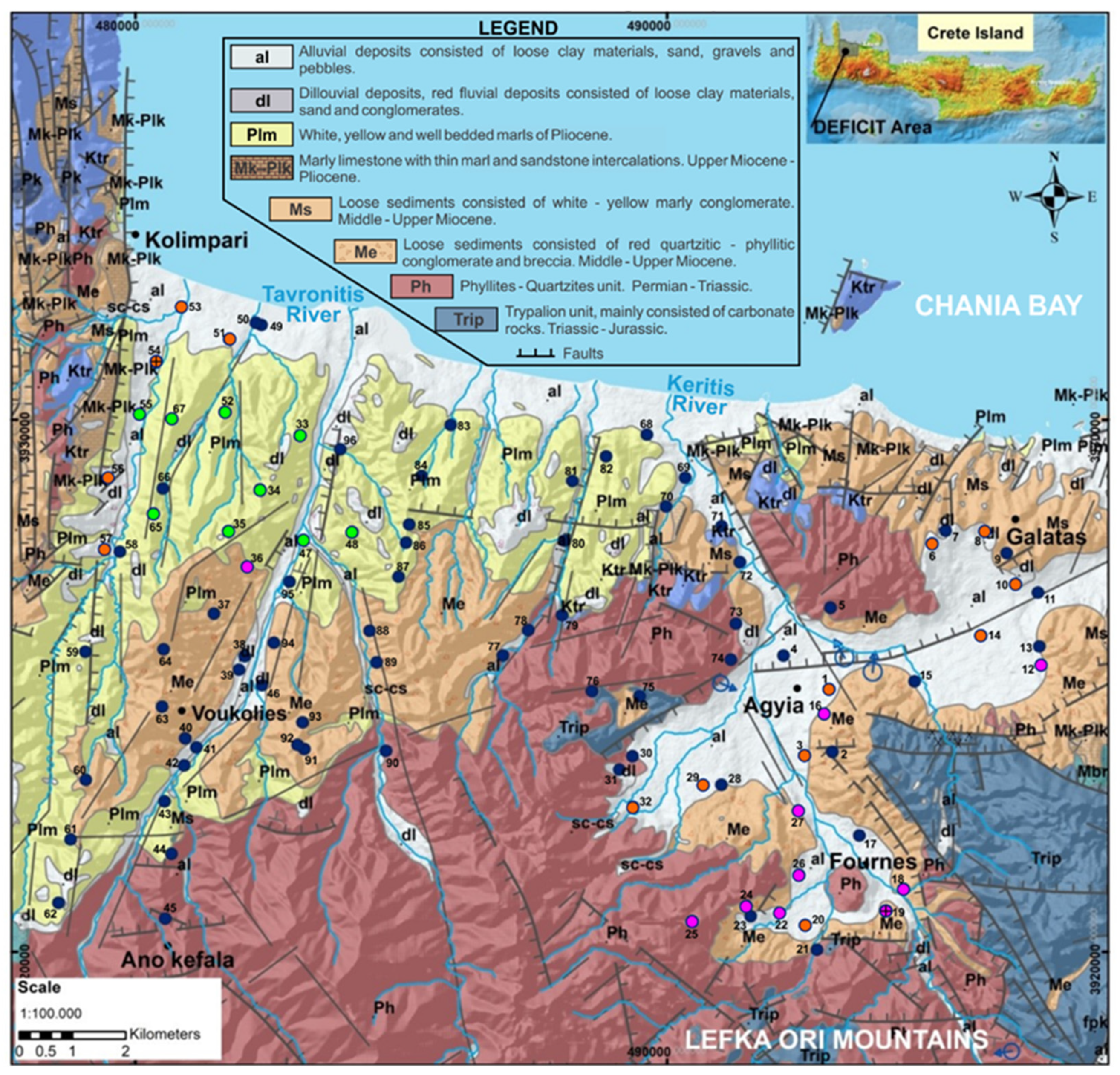
4.3. Agrogeology

Considering the findings of the agrogeophysical methods and soil analysis along with the geomorphological and geological structure of the study area, it is worth stressing that:

➢

70% of the members in S1, S2 and S3 classes are in altitudes below 100 m, and about 60% are in the vicinity of the hydrographic network.

➢

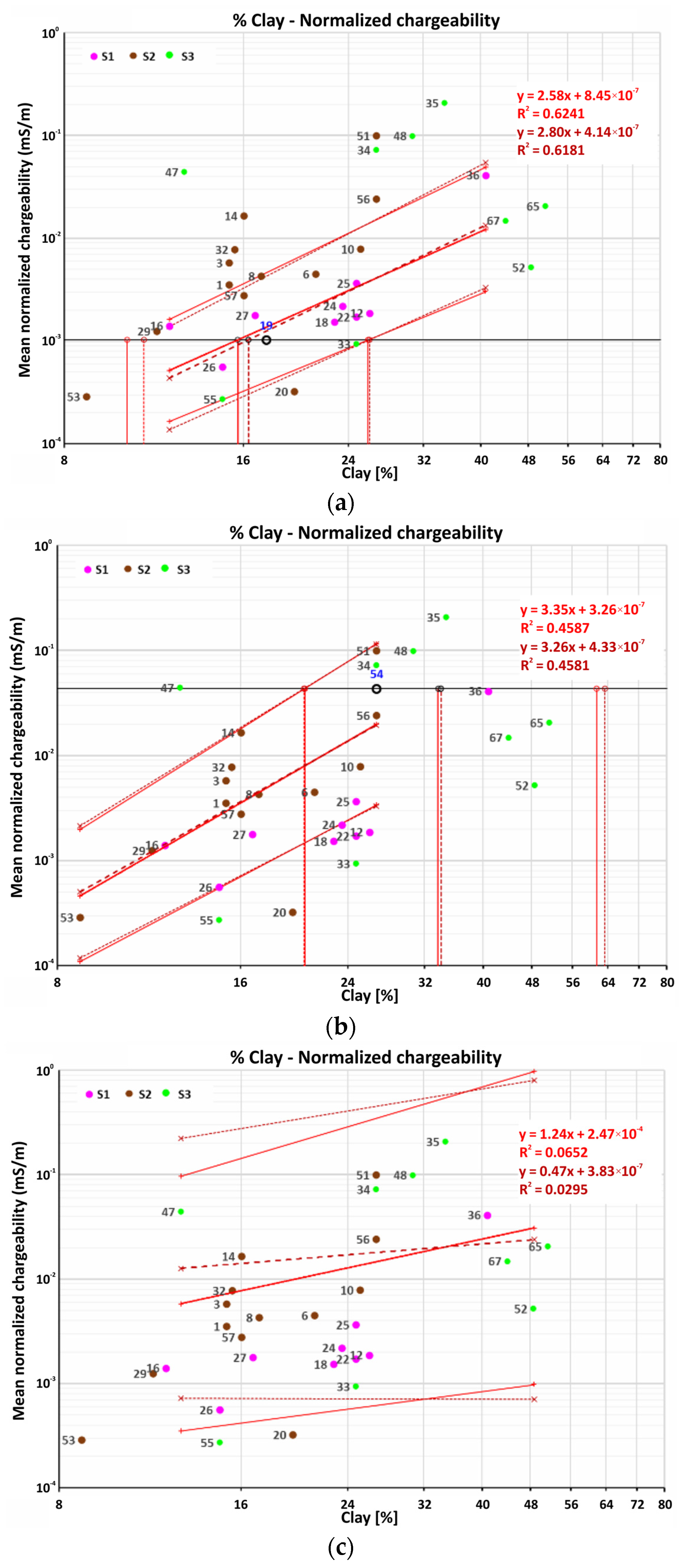
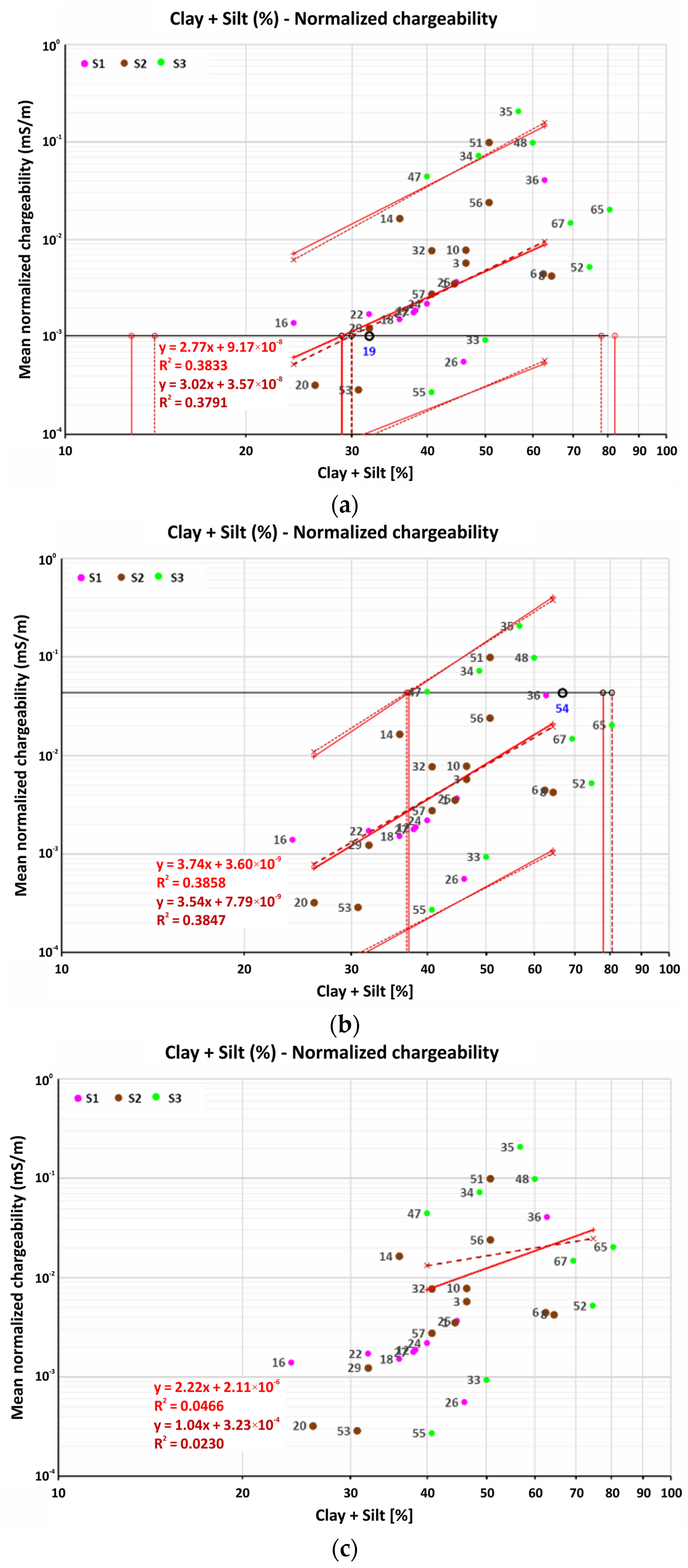
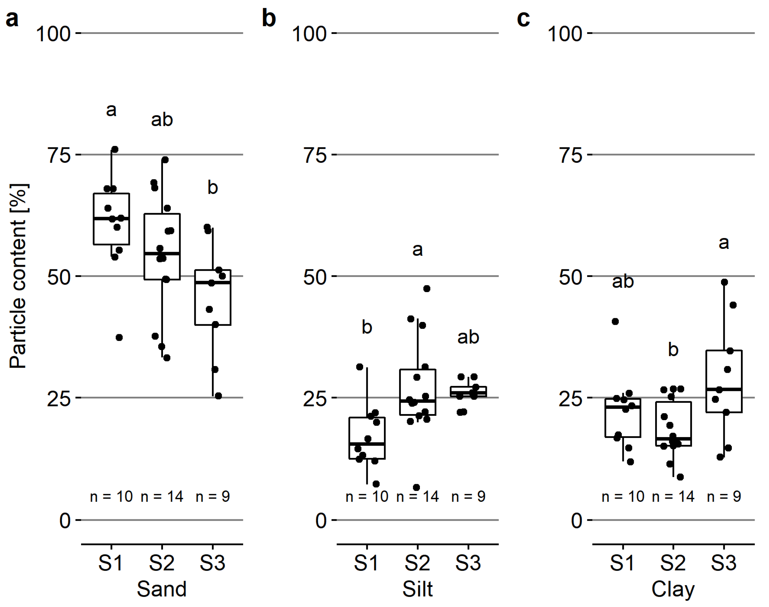
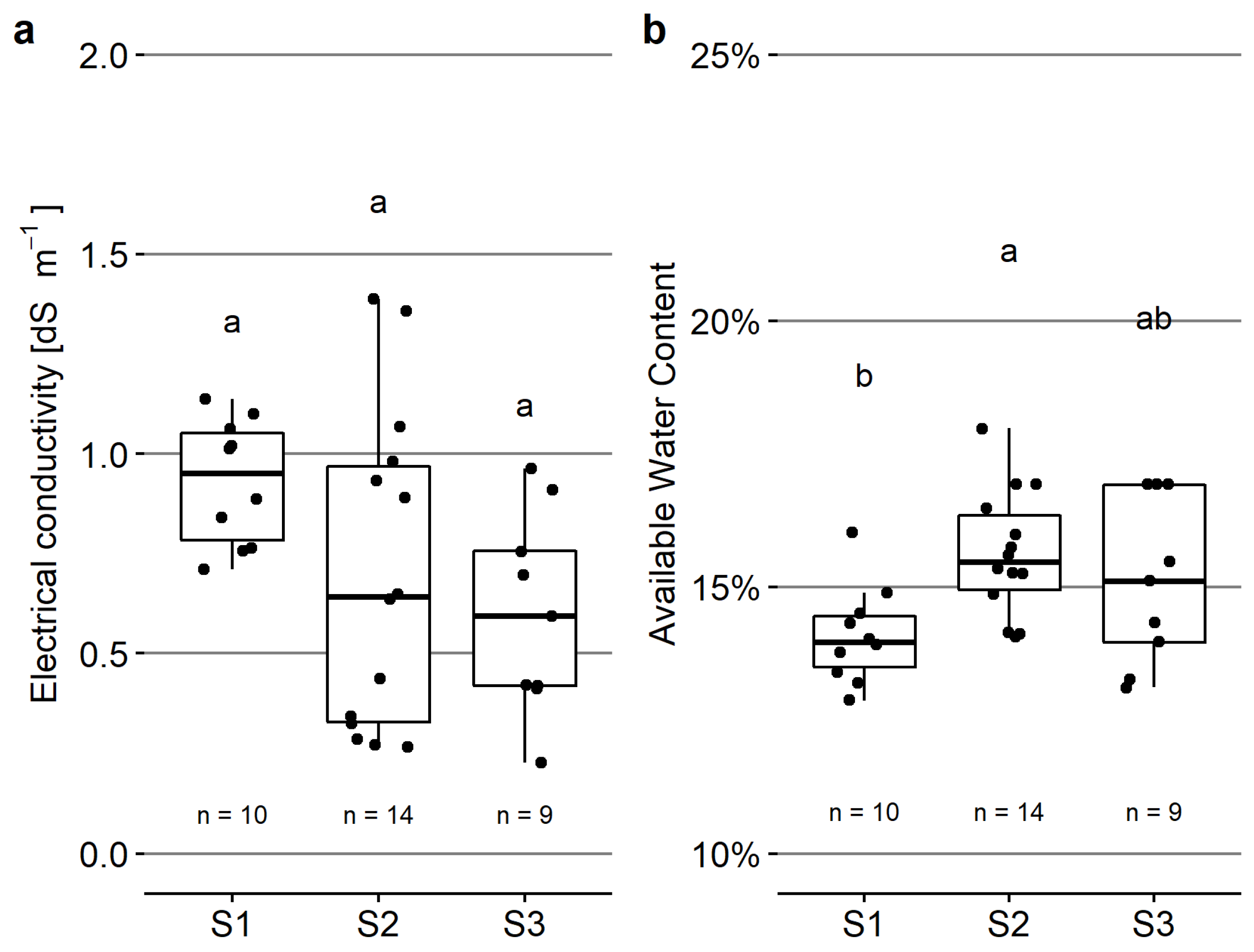
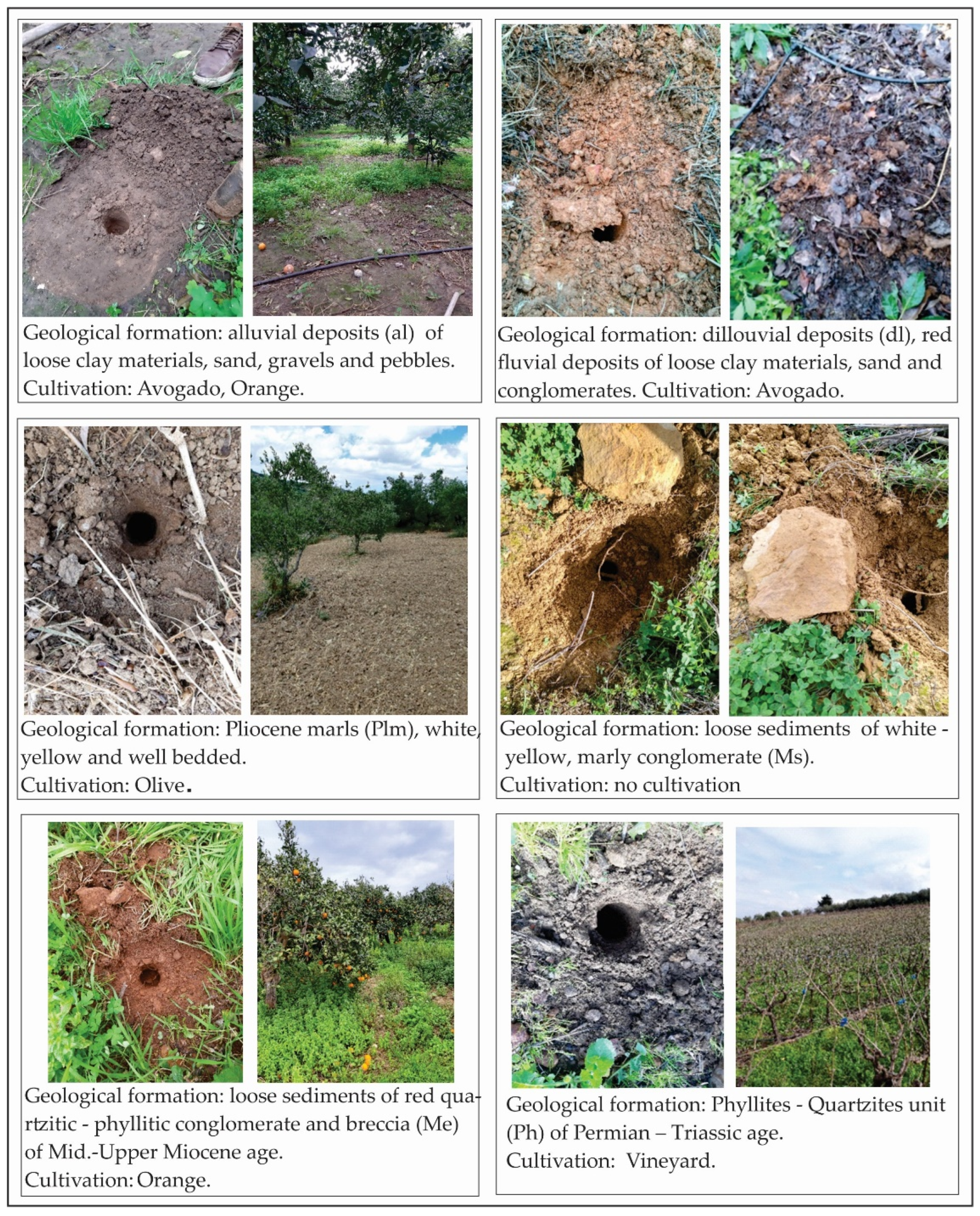
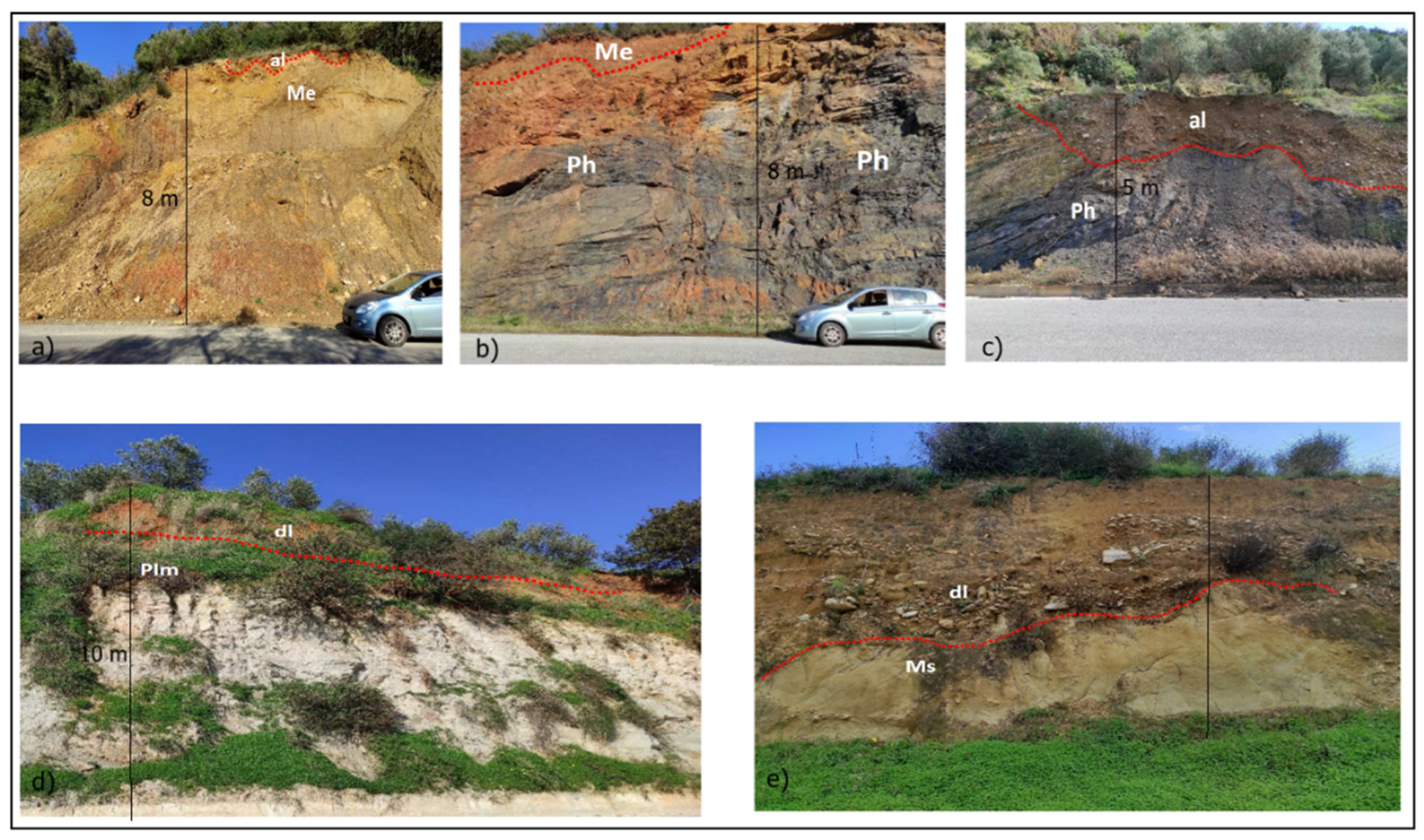
The S1 class, mainly present in the eastern part of the study area (Agyia), corresponds to formations older than Upper Miocene also including the transitional zone between the pre-Upper Miocene formations and the alluvial sediments. Specifically, the parent material of S1 class soils most probably is (a) the phyllite–quartzite unit (Ph) of the Permian–Triassic age and (b) the phyllitic–quartzitic conglomerate and breccia (Me) of the Middle-Upper Miocene. Furthermore, most (70%) S1 members belong to a cluster located in a small, closed basin (southeastern part of the Chania Plain–Fournes, Figure 2). This closed basin has been generated from the action of normal faults trending E–W, NW–SE, and NE–SW. The fault groups firmly control the ground slopes in the area around Fournes, thus facilitating the water movement and the transfer of erosional material from the parent rocks. The primary mineralogical component of the phyllitic–quartzitic material is quartz, while minor components are the clay minerals of muscovite and talc and rarely the gibbsite [79,80]. This supports the findings of the present, i.e., the sand content, apart from prevailing in all three classes, is also the highest for the S1 class (Figure 9). In addition, the S1 class corresponds to AWC, ranging between 12.5% and 15% (Figure 10), which is lower compared to the S2 and S3 classes. This is probably related to the fact that the phyllitic–quartzitic material is impermeable to water. Class S1 presents an improvement in the goodness of fit compared to the unclassified data. Thus, the predicted mean clay content at the test site (#19) of class S1 is considered acceptable (Table 2).

➢

The S2 class is present in the eastern and western part of the study area. It corresponds to Holocene and Pleistocene formations that include the alluvial (al) and dilluvial (dl) deposits and the transitional zones al-dl, al-Me and dl-Plm. Markopoulos et al. [81] collected samples of mudstones and soils from the wide area of the present study, aiming to evaluate their properties as raw materials. The soil particle distribution, plasticity, and the mineralogical content (through X-ray diffraction and calcimetry) were determined. Generally, quartz, illite, muscovite, chlorite, and calcite, with some Fe-minerals, feldspars and traces of gypsum, halite and anhydrite were identified in the samples, while clay minerals are between 30 to 50%. The high percentages of quartz and mica are because of the phyllite–quartzite unit in the area, while the presence of gypsum, anhydrite and halite is related to the deposition of marine sediments [82,83]. Especially for the Agyia (the eastern part of the study area), Markopoulos et al. [81] determined that the content was 79% sand, 13% clay and 8% silt. The interpretation of Markopoulos et al. [81] is supported by the findings of the present study. Specifically, the sand content of the S2 class members in this research ranges between 33% and 74%, and most of the members reveal sand content around 58%. Most of the S2 members reveal AWC higher than 15%, probably attributed to the nature of these alluvial sediments (high sand percentage, clay content ranging between 15 and 27%, high porosity, low compaction). Class S2 presents an improvement in the goodness of fit compared to the unclassified data. Consequently, the predicted mean clay content at the test site (#54) of class S2 is considered acceptable (Table 2).

➢

The S3 class is present in the western part of the study area, and it corresponds to the white and yellow well-bedded Pliocene marls of the Tavronitis Formation [84]. The upper part of this formation is a 25–50 cm thick layer of well-bedded medium-to-fine grained and brown soft sands, which alternates with massive white marls, interspersed with many unoriented worm tracks [85]. From the mineralogical point of view and considering the analogue of Pliocene marls for the Heraklion basin in central Crete [86], clay minerals are montmorillonite (up to 25%), illite (10–15%) and chlorite (less than 13%), while non-clay components are calcite (16–82%) and quartz (15–25%), with some grains of plagioclase and mica to be present. Furthermore, Tsiambaos [86] classified the Heraklion Pliocene marls in two groups, based on the calcium carbonate content. The marls of the first group are mainly marls and limey marls showing calcium carbonate content of 35–85%, and those of the second group are clayey marls revealing calcium carbonate content of 26–35%. These could possibly explain the findings of the present study, concerning class S3. The observed scattered clay content and AWC of class S3, compared to the other classes, shown in Figure 9 and Figure 10, might lead to low correlation between the normalized chargeability and the measured clay content. Furthermore, if class S3 consists mainly of limey marls, then it contains high sum of clay and silt content but a low concentration of clay minerals, which is the parameter that affects the normalized chargeability.

➢

The prediction of clay when the soil shows a small variation of clay content is another challenging part of this work. We show in this work that, in some cases, this can be feasible by taking into consideration geophysical and geological data as well.

4.4. Impact on Crop and Water Management

This empirical relationship between normalized chargeability and soil clay content in combination with the appropriate agrogeological soil classification can contribute to better crop-and-tree-planting planning and agricultural water management. The effect of soils on irrigation water requirement is essential to accurately evaluating regional water-saving potential and irrigation water needs [47,87]. Soils with different characteristics present significantly different irrigation times and total irrigation amounts. This is because of their different water-holding capacities, infiltration, water distribution in the soil profile and water retention time in the soil. While the volume of irrigation is a function of a combination of soil characteristics, plant growth stage and climate conditions, irrigation frequency depends only on soil characteristics [47]. The proposed approach facilitates a more efficient assessment of soil texture by allowing clay and the sum of clay and silt content to be estimated in 2-dimensional geophysical measurement cross-sections and potentially in 3-dimensional, rather than point-scale, samples. This improvement can contribute to better informed agricultural planning and agricultural decision support systems [88,89,90], as well as better strategic planning [60], which are essential for the Mediterranean.

The clay-based irrigation strategy is very different from the sand-based soil irrigation strategy. Clay-based soils have flat, small, compact particles with large surface-to-volume ratios. Thus, water is absorbed and moves slowly through clay soils, but they retain substantial amounts of moisture once wet. This means that water rapidly applied to clay soil tends to run off instead of moving into the ground. Therefore, when irrigating clay soils, water should be applied slowly for an extended period of time [45]. On the other hand, sand-based soils have large particles with a small surface-to-volume ratios. In these soils, water is absorbed and moves quickly beyond the root zone, making it unavailable to the plant and contributing to soil leaching. Thus, for sand-based soils, the irrigation dose should be applied in small quantities and more often (short intervals) [46].

In addition, as for drip irrigation system, the emitter flow rate can also be selected to accommodate different soil types, with high flow emitters used on sandy-based locations and low flow emitters on clay-based locations. Emitter distances can also vary, with longer distances in clay soils and shorter distances in sandy sites. Farmers using drip systems should take advantage of the above to maximize water-use efficiency [47]. As proposed in this study, easily applied field agrogeophysical and agrogeological approaches [91,92,93,94,95] can offer an accurate estimation of clay content for the upper soil layer (root zone soil depth), information, which is very important for farmers to apply the irrigation water to their plants with the proper frequency. In such cases, irrigation could be more efficient and environmentally safe.

5. Conclusions

In the present work, we explore the application of agrogeophysical properties (resistivity, conductivity, chargeability) assisted by agrogeological mapping and pedometrical analysis to both qualitatively and quantitatively characterize the arable fields in the plain of Chania in western Crete. Principal component analysis (PCA) in our case study failed to distribute a new measured position to the extracted from PCA analysis classes, while geologically based classification recognized three classes (S1, S2 and S3). The main conclusions from this research are:

• Agrogeophysical measurements aimed at investigating the clay or the sum of clay and silt soil content in medium-texture soils, such as in the arable fields of the Chania Plain, it is better to carry out the dry period of the year. This is because the effect of the water in the wet period of the year masks the influence of other factors (porosity, soil texture). The clay or the sum of clay and silt soil content within the investigated area can be successfully estimated by the normalized chargeability using induced polarization (IP) and resistivity measurements under dry conditions. Based on geological classification analysis for the above-mentioned measurements, we distinguished three classes (S1, S2 and S3) for the dry period data. For the first two classes (S1 and S2) associated with phyllites–quartzites, phyllitic–quartzitic conglomerate and breccia, and alluvial deposits, respectively, the estimation of clay or the sum of clay and silt soil content is feasible from measurements of the normalized chargeability. The S3 class, geologically related to Pliocene marls, is not statistically correlated to geoelectrical measurements. A denser network of geophysical measurements on Pliocene marls, distributed in the whole year, is required to check if normalized chargeability for clay content evaluation is suitable for Pliocene marls.
• The unpaired Wilcoxon test showed that classes S1, S2 and S3 present slight differences with respect to soil characteristics, while, according to the FAO European classification, they belong mainly to the medium texture. The sand content, relative to silt and clay contents, clearly prevails in all three classes. Considering the clay content, the S3 class presents the highest clay content compared to the S1 and S2 classes. In addition, classes S1 and S2 show differences with respect to available water content (AWC) probably attributed to the significant difference in the amount of silt in these classes. There are slight differences among the three classes considering the electrical conductivity.
• The S1 class mainly corresponds to formations older than the Upper Miocene, comprising the parent material of S1 class soils. These formations, older than the Upper Miocene, are (a) the phyllite–quartzite unit (Ph) of the Permian–Triassic age, and (b) the phyllitic–quartzitic conglomerate and breccia (Me) of the Middle-Upper Miocene. The primary mineralogical component of the phyllitic–quartzitic material is quartz, thus explaining the large (greater than 54%) sand content of S1 class members. The S2 class corresponds to Holocene and Pleistocene formations, including the alluvial (al) and dilluvial (dl) deposits and some transitional zones (al-dl, al-Me and dl-Plm). Most of the S2 class members reveal sand content around 58%. A reliable explanation for the high percentage of sand content in Holocene and Pliocene formations of S2 class members is the extended presence of the phyllite–quartzite unit that feeds with erosional material places of lower elevation in the study area. The S3 class corresponds to the Pliocene marls of the Tavronitis Formation, which exhibit scattered clay content and available water content (AWC), compared to the other classes. This might lead to low correlation between the normalized chargeability and the measured clay content in the data of class S3.

Future crop and tree planting planning and agricultural water strategy for the Chania Plain may consider the above findings since soil texture is significantly affected by the agrogeological characteristics in this area. The proposed combination of geophysical and geological approaches may be used to assess clay, the sum of clay and silt and, by extension, the available water content with significant detail in depth and scale. Soil texture should always be considered in the interpretation of the results. Probably, specialized geological analyses (such as mineralogical) could assist a more detailed characterization of the arable fields in the study area. Further work will concentrate on adding more observation points (collecting both soil samples and geophysical data) for all classes and performing analysis of the samples’ mineralogical content.

References

- Rossi, R. Irrigation in EU Agriculture; European Union: Brussels, Belgium, 2019. [Google Scholar]
- Huang, J.; Yu, H.; Guan, X.; Wang, G.; Guo, R. Accelerated Dryland Expansion under Climate Change. Nat. Clim. Chang. 2016, 6, 166–171. [Google Scholar] [CrossRef]
- Diffenbaugh, N.S.; Giorgi, F. Climate Change Hotspots in the CMIP5 Global Climate Model Ensemble. Clim. Chang. 2012, 114, 813–822. [Google Scholar] [CrossRef] [PubMed]
- Vrochidou, A.-E.; Tsanis, I.; Grillakis, M.; Koutroulis, A. The Impact of Climate Change on Hydrometeorological Droughts at a Basin Scale. J. Hydrol. 2012, 476, 290–301. [Google Scholar] [CrossRef]
- Chandler, D.G.; Seyfried, M.S.; McNamara, J.P.; Hwang, K. Inference of Soil Hydrologic Parameters from Electronic Soil Moisture Records. Front. Earth Sci. 2017, 5, 25. [Google Scholar] [CrossRef]
- Christias, P. A Comparative Study on Decision Support Approaches under Uncertainty. In Proceedings of the Lecture Notes in Business Information Processing; Springer: Berlin/Heidelberg, Germany, 2019; Volume 339, pp. 517–526. [Google Scholar]
- Phogat, V.; Skewes, M.A.; Cox, J.W.; Sanderson, G.; Alam, J.; Šimůnek, J. Seasonal Simulation of Water, Salinity and Nitrate Dynamics under Drip Irrigated Mandarin (Citrus Reticulata) and Assessing Management Options for Drainage and Nitrate Leaching. J. Hydrol. 2014, 513, 504–516. [Google Scholar] [CrossRef]
- Daliakopoulos, I.Ν.; Papadimitriou, D.; Matsoukas, T.; Zotos, N.; Moysiadis, H.; Anastasopoulos, K.; Mavrogiannis, I.; Manios, T. Development and Preliminary Results from the Testbed Infrastructure of the DRIP Project. Proceedings 2020, 30, 64. [Google Scholar] [CrossRef]
- Egea, G.; Diaz-Espejo, A.; Fernández, J.E. Soil Moisture Dynamics in a Hedgerow Olive Orchard under Well-Watered and Deficit Irrigation Regimes: Assessment, Prediction and Scenario Analysis. Agric. Water Manag. 2016, 164, 197–211. [Google Scholar] [CrossRef]
- Daliakopoulos, I.; Papadimitriou, D.; Manios, T. Improving the Efficiency of HYPROP by Controlling Temperature and Air Flow. In Proceedings of the EGU General Assembly Conference Abstracts, Online, 19–30 April 2021; p. EGU21-13082. [Google Scholar]
- Schelle, H.; Heise, L.; Jänicke, K.; Durner, W. Water Retention Characteristics of Soils over the Whole Moisture Range: A Comparison of Laboratory Methods. Eur. J. Soil Sci. 2013, 64, 814–821. [Google Scholar] [CrossRef]
- Koekkoek, E.J.W.; Booltink, H. Neural Network Models to Predict Soil Water Retention. Eur. J. Soil Sci. 1999, 50, 489–495. [Google Scholar] [CrossRef]
- Ghanbarian-alavijeh, B.; Liaghat, A.; Huang, G.-H.; Van Genuchten, M.T. Estimation of the van Genuchten Soil Water Retention Properties from Soil Textural Data. Pedosphere 2010, 20, 456–465. [Google Scholar] [CrossRef]
- Schaap, M.G.; Leij, F.J.; van Genuchten, M.T. Rosetta: A Computer Program for Estimating Soil Hydraulic Parameters with Hierarchical Pedotransfer Functions. J. Hydrol. 2001, 251, 163–176. [Google Scholar] [CrossRef]
- Hengl, T.; de Jesus, J.M.; MacMillan, R.A.; Batjes, N.H.; Heuvelink, G.B.M.; Ribeiro, E.; Samuel-Rosa, A.; Kempen, B.; Leenaars, J.G.B.; Walsh, M.G.; et al. SoilGrids1km—Global Soil Information Based on Automated Mapping. PLoS ONE 2014, 9, e105992. [Google Scholar] [CrossRef] [PubMed]
- Batjes, N.H. Harmonized Soil Profile Data for Applications at Global and Continental Scales: Updates to the WISE Database. Soil Use Manag. 2009, 25, 124–127. [Google Scholar] [CrossRef]
- Grillakis, M.G.; Koutroulis, A.G.; Alexakis, D.D.; Polykretis, C.; Daliakopoulos, I.N. Regionalizing Root-Zone Soil Moisture Estimates From ESA CCI Soil Water Index Using Machine Learning and Information on Soil, Vegetation, and Climate. Water Resour. Res. 2021, 57, e2020WR029249. [Google Scholar] [CrossRef]
- Babaeian, E.; Homaee, M.; Vereecken, H.; Montzka, C.; Norouzi, A.A.; van Genuchten, M.T. A Comparative Study of Multiple Approaches for Predicting the Soil-Water Retention Curve: Hyperspectral Information vs. Basic Soil Properties. Soil Sci. Soc. Am. J. 2015, 79, 1043–1058. [Google Scholar] [CrossRef]
- Ulaby, F.T.; Bradley, G.A.; Dobson, M.C. Microwave Backscatter Dependence on Surface Roughness, Soil Moisture, and Soil Texture: Part II-Vegetation-Covered Soil. IEEE Trans. Geosci. Electron. 1979, 17, 33–40. [Google Scholar] [CrossRef]
- Ulaby, F.T.; Batlivala, P.P.; Dobson, M.C. Microwave Backscatter Dependence on Surface Roughness, Soil Moisture, and Soil Texture: Part I-Bare Soil. IEEE Trans. Geosci. Electron. 1978, 16, 286–295. [Google Scholar] [CrossRef]
- Alexakis, D.D.D.; Mexis, F.-D.K.F.D.K.; Vozinaki, A.-E.K.A.E.K.; Daliakopoulos, I.N.I.N.; Tsanis, I.K.I.K. Soil Moisture Content Estimation Based on Sentinel-1 and Auxiliary Earth Observation Products. A Hydrological Approach. Sensors 2017, 17, 1455. [Google Scholar] [CrossRef]
- De Melo, L.B.B.; Silva, B.M.; Peixoto, D.S.; Chiarini, T.P.A.; de Oliveira, G.C.; Curi, N. Effect of Compaction on the Relationship between Electrical Resistivity and Soil Water Content in Oxisol. Soil Tillage Res. 2021, 208, 104876. [Google Scholar] [CrossRef]
- Klotzsche, A.; Lärm, L.; Vanderborght, J.; Cai, G.; Morandage, S.; Zörner, M.; Vereecken, H.; Kruk, J. Monitoring Soil Water Content Using Time-Lapse Horizontal Borehole GPR Data at the Field-Plot Scale. Vadose Zone J. 2019, 18, 190044. [Google Scholar] [CrossRef] [Green Version]
- Economou, N.; Brintakis, J.; Andronikidis, N.; Kritikakis, G.; Kokkinou, E.; Papadopoulos, N.; Kourgialas, N.; Vafidis, A. Gpr Data Migration Velocity Estimation Using a Local Diffraction Multi-Focusing Criterion. In Proceedings of the 11th Congress of the Balkan Geophysical Society, Online, 10–14 October 2021; European Association of Geoscientists & Engineers: Bunnik, The Netherlands; pp. 1–5. [Google Scholar]
- Archie, G.E. The Electrical Resistivity Log as an Aid in Determining Some Reservoir Characteristics. Trans. AIME 1942, 146, 54–62. [Google Scholar] [CrossRef]
- Waxman, M.H.; Smits, L.J.M. Electrical Conductivities in Oil-Bearing Shaly Sands. Soc. Pet. Eng. J. 1968, 8, 107–122. [Google Scholar] [CrossRef]
- Linde, N.; Binley, A.; Tryggvason, A.; Pedersen, L.B.; Revil, A. Improved Hydrogeophysical Characterization Using Joint Inversion of Cross-Hole Electrical Resistance and Ground-Penetrating Radar Traveltime Data. Water Resour. Res. 2006, 42. [Google Scholar] [CrossRef]
- Soupios, P.M.; Kouli, M.; Vallianatos, F.; Vafidis, A.; Stavroulakis, G. Estimation of Aquifer Hydraulic Parameters from Surficial Geophysical Methods: A Case Study of Keritis Basin in Chania (Crete—Greece). J. Hydrol. 2007, 338. [Google Scholar] [CrossRef]
- Vinegar, H.J.; Waxman, M.H. Induced Polarization of Shaly Sands. Geophysics 1984, 49, 1267–1287. [Google Scholar] [CrossRef]
- Kemna, A.; Binley, A.; Cassiani, G.; Niederleithinger, E.; Revil, A.; Slater, L.; Williams, K.H.; Orozco, A.F.; Haegel, F.-H.; Hördt, A.; et al. An Overview of the Spectral Induced Polarization Method for Near-Surface Applications. Near Surf. Geophys. 2012, 10, 453–468. [Google Scholar] [CrossRef]
- Slater, L. Near Surface Electrical Characterization of Hydraulic Conductivity: From Petrophysical Properties to Aquifer Geometries—A Review. Surv. Geophys. 2007, 28, 169–197. [Google Scholar] [CrossRef]
- Ntarlagiannis, D.; Doherty, R.; Costa, R.; Williams, K.H.; Zhang, C.; Soupios, P. Introduction to Special Section: Characterization and Monitoring of Subsurface Contamination. Interpretation 2015, 3, 2324–8858. [Google Scholar] [CrossRef]
- Ntarlagiannis, D.; Robinson, J.; Soupios, P.; Slater, L. Field-Scale Electrical Geophysics over an Olive Oil Mill Waste Deposition Site: Evaluating the Information Content of Resistivity versus Induced Polarization (IP) Images for Delineating the Spatial Extent of Organic Contamination. J. Appl. Geophys. 2016, 135, 418–426. [Google Scholar] [CrossRef]
- Revil, A.; Razdan, M.; Julien, S.; Coperey, A.; Abdulsamad, F.; Ghorbani, A.; Gasquet, D.; Sharma, R.; Rossi, M. Induced Polarization Response of Porous Media with Metallic Particles—Part 9: Influence of Permafrost. Geophysics 2019, 84, E337–E355. [Google Scholar] [CrossRef]
- Revil, A.; Qi, Y.; Ghorbani, A.; Coperey, A.; Ahmed, A.S.; Finizola, A.; Ricci, T. Induced Polarization of Volcanic Rocks. 3. Imaging Clay Cap Properties in Geothermal Fields. Geophys. J. Int. 2019, 218, 1398–1427. [Google Scholar] [CrossRef]
- Garré, S.; Hyndman, D.; Mary, B.; Werban, U. Geophysics Conquering New Territories: The Rise of “Agrogeophysics”. Vadose Zone J. 2021, 20, e20115. [Google Scholar] [CrossRef]
- Woodward, H. Geology and Agricutlure. Nature 1869, 46–48. [Google Scholar] [CrossRef]
- Gough, L.P.; Herring, J.R. Geologic Research in Support of Sustainable Agriculture. Agric. Ecosyst. Environ. 1993, 46, 55–68. [Google Scholar] [CrossRef]
- Lin, H. Earth’s Critical Zone and Hydropedology: Concepts, Characteristics, and Advances. Hydrol. Earth Syst. Sci. 2010, 14, 25–45. [Google Scholar] [CrossRef]
- Zeng, Q.; Ma, X.; Peng, P.; Xu, W.; Feng, X.; Wei, R.; Huang, X.; Qi, T.; Xiaofeng, W. Limei Pan Agrogeological Investigation on the Original Producing Area of Siraitia Grosvenorii. In Proceedings of the 2011 International Conference on Multimedia Technology, Melbourne, Australia, 19–20 November 2011; IEEE: Piscataway, NJ, USA, 2011; pp. 5264–5267. [Google Scholar]
- Gill, J.C. Geology and the Sustainable Development Goals. Episodes 2017, 40, 70–76. [Google Scholar] [CrossRef]
- Jones, J.M.C.; Guinel, F.C.; Antunes, P.M. Carbonatites as Rock Fertilizers: A Review. Rhizosphere 2020, 13, 100188. [Google Scholar] [CrossRef]
- Bouyoucos, G.J. The Hydrometer as a New Method for the Mechanical Analysis of the Soil. Soil Sci. 1927, 23, 343–349. [Google Scholar] [CrossRef]
- Bouyoucos, G.J. A Recalibration of the Hydrometer Method for Making Mechanical Analysis of Soils. Agron. J. 1951, 43, 434–438. [Google Scholar] [CrossRef]
- Katerji, N.; Mastrorilli, M. The Effect of Soil Texture on the Water Use Efficiency of Irrigated Crops: Results of a Multi-Year Experiment Carried out in the Mediterranean Region. Eur. J. Agron. 2009, 30, 95–100. [Google Scholar] [CrossRef]
- Katerji, N.; Mastrorilli, M.; Cherni, H.E. Effects of Corn Deficit Irrigation and Soil Properties on Water Use Efficiency. A 25-Year Analysis of a Mediterranean Environment Using the STICS Model. Eur. J. Agron. 2010, 32, 177–185. [Google Scholar] [CrossRef]
- Fang, J.; Su, Y. Effects of Soils and Irrigation Volume on Maize Yield, Irrigation Water Productivity, and Nitrogen Uptake. Sci. Rep. 2019, 9, 7740. [Google Scholar] [CrossRef] [PubMed]
- Daliakopoulos, I.N.; Panagea, I.S.; Tsanis, I.K.; Grillakis, M.G.; Koutroulis, A.G.; Hessel, R.; Mayor, A.G.; Ritsema, C.J. Yield Response of Mediterranean Rangelands under a Changing Climate. Land Degrad. Dev. 2017, 28, 1962–1972. [Google Scholar] [CrossRef]
- Pavlakis, P. Contribution to the Hydrogeological Investigation of the Calcareous Aquifer of Agyia Springs; Aristotle University of Thessaloniki: Thessaloniki, Greece, 1989. [Google Scholar]
- Pavlaki, A. Engineering Geological Conditions in Chania Prefecture, Crete Island; Aristotle University of Thessaloniki: Crete, Greece, 2008. [Google Scholar]
- Pavlaki, A.; Meladiotis, I.; Pavlakis, P. Applicability of the "Lefka Ori" Western Crete region "GeoFactors" Interaction Matrix (GFIM) as a key to understanding the engineering geological condtions. Bull. Geol. Soc. Greece 2013, 47, 1820–1833. [Google Scholar] [CrossRef]
- Mountrakis, D.; Kilias, A.; Pavlaki, A.; Fassoulas, C.; Thomaidou, E.; Papazachos, C.; Papaioannou, C.; Roumelioti, Z.; Benetatos, C.; Vamvakaris, D. Neotectonic Study of the Western Crete and Implications for Seismic Hazard Assessment. J. Virtual Explor. 2012, 42, 2. [Google Scholar] [CrossRef]
- Fytrolakis, N. The Geological Structure of Crete; University of Athens: Athens, Greece, 1980. [Google Scholar]
- Kilias, A.; Fassoulas, C.; Mountrakis, D. Tertiary Extension of Continental Crust and Uplift of Psiloritis Metamorphic Core Complex in the Central Part of the Hellenic Arc (Crete, Greece). In Active Continental Margins—Present and Past; Springer: Berlin, Heidelberg, 1994; pp. 417–430. [Google Scholar]
- Fassoulas, C.; Kilias, A.; Mountrakis, D. Postnappe Stacking Extension and Exhumation of High-Pressure/Low-Temperature Rocks in the Island of Crete, Greece. Tectonics 1994, 13, 127–138. [Google Scholar] [CrossRef]
- Pavlakis, P. Water Resources of Crete. Unified Transport Planning & Management—Water Schemes. In Proceedings of the Development, Spatial Planning and Environment; Technical Chamber of Greece, Department of Eastern Crete: Heraklion, Greece, 2007. [Google Scholar]
- Pavlakis, A.P. Water Resources Planning & Management Schemes of Crete. Potential for Increasing Available Water Resources in Western Crete. In Proceedings of the 11th ICOLD European Club Symposium, Chania, Greece, 2–4 October 2019. [Google Scholar]
- Koutroulis, A.G.A.; Grillakis, M.G.M.; Daliakopoulos, I.N.I.; Tsanis, I.I.K.; Jacob, D. Cross Sectoral Impacts on Water Availability at +2 °C and +3 °C for East Mediterranean Island States: The Case of Crete. J. Hydrol. 2016, 532, 16–28. [Google Scholar] [CrossRef]
- Koutroulis, A.G.; Tsanis, I.K.; Daliakopoulos, I.N.; Jacob, D. Impact of Climate Change on Water Resources Status: A Case Study for Crete Island, Greece. J. Hydrol. 2013, 479, 146–158. [Google Scholar] [CrossRef]
- Demetropoulou, L.; Lilli, M.A.; Petousi, I.; Nikolaou, T.; Fountoulakis, M.; Kritsotakis, M.; Panakoulia, S.; Giannakis, G.V.; Manios, T.; Nikolaidis, N.P. Innovative Methodology for the Prioritization of the Program of Measures for Integrated Water Resources Management of the Region of Crete, Greece. Sci. Total Environ. 2019, 672, 61–70. [Google Scholar] [CrossRef]
- Pavlakis, A.P.; Lydakis, N.S. Exploitation of the Important Water Resources in Chania Prefecture, in Order to Meet the Irrigation & Water Supply Demands. In Proceedings of the Conference Promotion of Development & Environmental Infrastructure Projects—ESPA 2007–2013; Technical Chamber of Greece, Department of Western Crete: Chania, Greece, 2010. [Google Scholar]
- Pavlakis, P. The Major Hydraulic Projects of Crete. Available Water Resources Projects’ Management. In Dams and Reservoirs in Crete: Design, Construction & Management of Large Hydraulic Works; OAK: Heraklion, Greece, 2014. [Google Scholar]
- Dahlin, T.; Zhou, B. Multiple-Gradient Array Measurements for Multichannel 2D Resistivity Imaging. Near Surf. Geophys. 2006, 4, 113–123. [Google Scholar] [CrossRef] [Green Version]
- Rengasamy, P. World Salinization with Emphasis on Australia. J. Exp. Bot. 2006, 57, 1017–1023. [Google Scholar] [CrossRef] [PubMed]
- Beaudette, D.; Skovlin, J.; Roecker, S.; Brown, A. Maintainer, Package “SoilDB”. Soil Database Interface. R Package Version 2.7.2. 2022. Available online: https://CRAN.R-project.org/package=soilDB (accessed on 1 June 2022).
- Zhang, Y.; Schaap, M.G. Weighted Recalibration of the Rosetta Pedotransfer Model with Improved Estimates of Hydraulic Parameter Distributions and Summary Statistics (Rosetta3). J. Hydrol. 2017, 547, 39–53. [Google Scholar] [CrossRef]
- Telford, W.M.; William, M.; Geldart, L.P.; Sheriff, R.E. Applied Geophysics; Cambridge University Press: Cambridge, UK, 1990. [Google Scholar] [CrossRef]
- Friedman, S.P. Soil Properties Influencing Apparent Electrical Conductivity: A Review. Comput. Electron. Agric. 2005, 46, 45–70. [Google Scholar] [CrossRef]
- Draper, N.R.; Smith, H. Applied Regression Analysis; Wiley: West Maitland, FL, USA, 1998; ISBN 978-0-471-17082-2. [Google Scholar]
- Cohen, A.; Migliorati, G. Optimal Weighted Least-Squares Methods. SMAI J. Comput. Math. 2017, 3, 181–203. [Google Scholar] [CrossRef]
- Davydenko, A.Y.; Grayver, A.V. Principal Component Analysis for Filtering and Leveling of Geophysical Data. J. Appl. Geophys. 2014, 109, 266–280. [Google Scholar] [CrossRef]
- Mao, D.; Revil, A.; Hinton, J. Induced Polarization Response of Porous Media with Metallic Particles—Part 4: Detection of Metallic and Nonmetallic Targets in Time-Domain Induced Polarization Tomography. Geophysics 2016, 81, D359–D375. [Google Scholar] [CrossRef]
- Revil, A.; Gresse, M. Induced Polarization as a Tool to Assess Alteration in Geothermal Systems: A Review. Minerals 2021, 11, 962. [Google Scholar] [CrossRef]
- Gonzales, A.A.; Dahlin, T.; Barmen, G.; Rosberg, J.-E. Electrical Resistivity Tomography and Induced Polarization for Mapping the Subsurface of Alluvial Fans: A Case Study in Punata (Bolivia). Geosciences 2016, 6, 51. [Google Scholar] [CrossRef]
- Slater, L.D.; Lesmes, D. IP Interpretation in Environmental Investigations. Geophysics 2002, 67, 77–88. [Google Scholar] [CrossRef]
- Lesmes, D.P.; Friedman, S.P. Relationships between the Electrical and Hydrogeological Properties of Rocks and Soils. In Hydrogeophysics; Rubin, Y., Hubbard, S.S., Eds.; Springer: Dordrecht, The Netherlands, 2005; Volume 50. [Google Scholar] [CrossRef]
- European Soil Bureau. Georeferenced Soil Database for Europe; European Soil Bureau and Joint Research Centre, EC.: Ispra, Italy, 1998. [Google Scholar]
- Phocaides, A. Handbook on Pressurized Irrigation Techniques; Food and Agriculture Organization of the United Nations (FAO): Rome, Italy, 2007. [Google Scholar]
- Dornsiepen, U.F.; Manutsoglu, E. On the Subdivision of the Phyllite-Nappe of Crete and Peloponnesus. Z. Dtsch. Geol. Ges. 1994, 145, 286–304. [Google Scholar] [CrossRef]
- Trichos, D.; Alevizos, G.; Stratakis, A.; Petrakis, E.; Galetakis, M. Mineralogical Investigation and Mineral Processing of Iron Ore from the Skines Area (Chania—West Crete). Bull. Geol. Soc. Greece 2016, 47, 1652. [Google Scholar] [CrossRef]
- Markopoulos, T.; Rotondo, P.; Chrysafaki, G.; Mousourakis, A. Evaluation of Mudstone Formations from Crete and Their Suitability for Rammed Earth and Adobe Production. Proc. Sci. Conf. SGEM 2008, 1, 659–673. [Google Scholar]
- Frydas, D.; Keupp, H. Biostratigraphical Results in Late Neogene Deposits of NW Crete, Greece, Based on Calcareous Nannofossils. Berl. Geowiss. Abh. 1996, 169–189. [Google Scholar]
- Frydas, D.; Keupp, H.; Bellas, S. Biostratigraphical Research in Late Neogene Marine Deposits of the Chania Province. Berl. Geowiss. Abh. 1999, E30, 55–67. [Google Scholar]
- Frydas, D. Calcareous and Siliceous Phytoplankton Stratigraphy of Neogene Marine Sediments in Central Crete (Greece). Rev. Micropaléontologie 2004, 47, 87–102. [Google Scholar] [CrossRef]
- Freudenthal, T. Stratigraphy of Neogene Deposits in the Khania Province, Crete, with Special Reference to Foraminifera of the Family Planorbulinidae and the Genus Heterostegina. Ph.D. Thesis, Utrecht University, Utrecht, The Netherlands, 1969. [Google Scholar]
- Tsiambaos, G. Correlation of Mineralogy and Index Properties with Residual Strength of Iraklion Marls. Eng. Geol. 1991, 30, 357–369. [Google Scholar] [CrossRef]
- Ali, M.H.; Talukder, M.S.U. Increasing Water Productivity in Crop Production—A Synthesis. Agric. Water Manag. 2008, 95, 1201–1213. [Google Scholar] [CrossRef]
- Christias, P.; Daliakopoulos, I.N.; Manios, T.; Mocanu, M. Comparison of Three Computational Approaches for Tree Crop Irrigation Decision Support. Math 2020, 8, 717. [Google Scholar] [CrossRef]
- Petousi, I.; Daliakopoulos, I.N.; Matsoukas, T.; Zotos, N.; Mavrogiannis, I.; Manios, T. DRIP: Development of an Advanced Precision Drip Irrigation System for Tree Crops. Terraenvision Abstr. 2018, 1, 2018–2022. [Google Scholar]
- Kourgialas, N.N.; Koubouris, G.C.; Dokou, Z. Optimal Irrigation Planning for Addressing Current or Future Water Scarcity in Mediterranean Tree Crops. Sci. Total Environ. 2019, 654, 616–632. [Google Scholar] [CrossRef]
- Chesworth, W.; van Straaten, P.; Semoka, J.M.R. Agrogeology in East Africa: The Tanzania-Canada project. J. Afr. Earth Sci. 1989, 9, 357–362. [Google Scholar] [CrossRef]
- Van Straaten, P. Rocks for Crops: Agrominerals of Sub-Saharan Africa; ICRAF: Nairobi, Kenya, 2002. [Google Scholar]
- Corwin, D.L.; Lesch, S.M. Apparent soil electrical conductivity measurements in agriculture. Comput. Electron. Agric. 2005, 46, 11–43. [Google Scholar] [CrossRef]
- Allred, B.J.; Daniels, J.J.; Ehsani, M.R. Handbook of Agricultural Geophysics; CRC Press: Boca Raton, FL, USA, 2008. [Google Scholar] [CrossRef]
- Guo, L.; Chen, J.; Cui, X.; Fan, B.; Lin, H. Application of ground penetrating radar for coarse root detection and quantification: A review. Plant Soil 2012, 362, 1–23. [Google Scholar] [CrossRef] [Green Version]