
Implementation of TETIS Hydrologic Model into the Hillslope Link Model Framework


Iowa Flood Center, IIHR-Hydroscience and Engineering, 323 Maxwell Stanley Hydraulics Laboratory, University of Iowa, Iowa City, IA 52245, USA
*
Author to whom correspondence should be addressed.
Water 2022, 14(17), 2610; https://doi.org/10.3390/w14172610
Submission received: 22 July 2022
/
Revised: 19 August 2022
/
Accepted: 20 August 2022
/
Published: 25 August 2022
(This article belongs to the Section Hydrology)
Abstract
:This communication introduces HLM-Tetis, which is a model structure coupled to the Hillslope Link Model (HLM) framework developed by the Iowa Flood Center. The model was designed to improve some limitations of previous HLM model structures. The following changes have been made: (1) modules to simulate snow processes; (2) better flexibility to simulate infiltration and percolation; (3) more flexibility to derive total runoff from the partitioning of overland flow, interflow and baseflow components. We show applications of the model in flood events at five basins in Iowa where previous model structures had performance limitations.
1. Introduction
The Iowa Flood Center at the University of Iowa developed a framework for hydrologic modeling known as the Hillslope Link Model (HLM). The modeling system is oriented to anticipate flood events, which is one of the most prevalent natural disasters, leading to mortality and significant economic losses in infrastructure and agriculture [1,2,3,4]. HLM is based on the decomposition of the landscape into hillslopes and channels. The hillslope is the hydrologic response unit where the runoff generation processes take place; the channel is where water is routed across the river network. Hydrologic models’ structures can be added into HLM by implementing the ordinary differential equations that describe the conversion of rainfall into runoff through soil moisture accounting at each hillslope and the routing of flow in the channels across the river network [5]. To solve the system of ordinary differential equations, HLM includes a numerical solver that offers variable size through an error control structure and is compatible with a High-Performance Computing framework [6].
1.1. Deficiencies of Previous Models
Different model structures have been added to HLM over time, with varying levels of complexity and model forcings [7,8,9,10]. The models have been extensively been evaluated in basins in the state of Iowa, USA, where they are used to provide flood forecasting. The models have been examined using offline comparing simulations with streamflow observations at 140 basins, which range between 10 and 40,000 km2, using different metrics such as Kling Gupta Efficiency, Nash Efficiency, peak flow bias, volume bias and others [11]. The models have been examined using different precipitation products, including Stage IV [12] precipitation data from 2002 to the present. The performance of the models has been also tested using the Iowa Flood Center radar-based precipitation product, version 5 [13].
Previous literature studies [11,14] found that models implemented in HLM have good overall skill in reproducing the fluctuations of streamflow and the annual maxima [11,14]. However, these studies also allowed detecting deficiencies of the models that led to poor performance in specific regions and type of event. These deficiencies include:
1.1.1. Model Performance in Western Iowa
Past examination of the models in basins of Western Iowa showed poor performance [11]. The basins in this region are characterized for having steep hills and man-made channels, which lead to faster overland flow in the hillslope surface and faster flow in the channels in the river network. The previous model structures implemented in HLM did not perform well at modeling these conditions, even after changing model parameterization.
1.1.2. Model Performance in Des Moines Lobe
A similar performance issue is found at basins in the Des Moines Lobe landform, which is characterized by having shallow soils with perennial river networks.
1.1.3. Flow Events Governed by Snowmelt
Many basins in Iowa, including those in the Des Moines Lobe and Western Iowa, are covered by snow in winter and spring months. During the cold season of the year, runoff generation is governed by snowmelt processes, and infiltration is controlled by frozen ground. Previous model structures in HLM did not include a snowmelt and frozen ground component.
1.2. Development of a New Model and Novel Contribution
In this study, the authors implemented a new model structure designed to overcome the deficiencies described in the previous section. The new model is called HLM-Tetis, honoring the name of a model with similar structure created by a former mentor of the authors [15,16]. A novel contribution of our paper is that the model structure is implemented in the Hillslope Link framework; that is, all the runoff generation processes occur at the hillslope scale, in contrast to the pixel scale of the original Tetis model. In a similar way, a novelty of our work is that the routing component uses channel links as control volume compared to the gridded representation of the river network used in the original implementation of Tetis. The advantages of using a hillslope link structure for hydrologic modeling are presented in detail in [5]. The model structure and its forcings are described in the Materials and Methods section. We propose an experiment to evaluate the model performance and compare it with previous models available in HLM.
2. Materials and Methods
2.1. The Hillslope Link Model Framework
The Hillslope Link Model (HLM) is a framework for hydrologic simulation that is based on the decomposition of the landscape into hillslopes and river channels. The hillslope is the hydrologic response unit where the runoff generation processes occur. The channel is the control volume where water produced in the hillslope is routed across the river network. Hydrological model structures are added into HLM by implementing the ordinary differential equations that describe the runoff generation at each hillslope and the routing at each channel. To solve the resultant system of ordinary differential equations, HLM includes a numerical solver that offers variable size through an error control structure and is compatible with a High-Performance Computing framework [6]. In this paper, we propose a new model structure described next.
2.2. Model Forcings
The new model uses five forcings: (1) rainfall, (2) actual evapotranspiration, (3) air temperature, (4) frozen ground, and (5) observed discharge. Inputs can be forced at any temporal resolution as long as they match the units required by the model. Inputs can be also forced uniformly for all the spatial domain or distributed as the forcing of each hillslope. Rainfall is forced as intensity in mm per hour, evapotranspiration in mm per month, and air temperature in Celsius degrees. Frozen ground is a binary variable (0 or 1) describing if the soil surface is frozen (1) or not (0). Observed discharge can be optionally forced into the model in m3/s and can be used to incorporate the data of reservoir operation or to assimilate streamflow data from measurement gages.
2.3. Runoff Generation and Routing
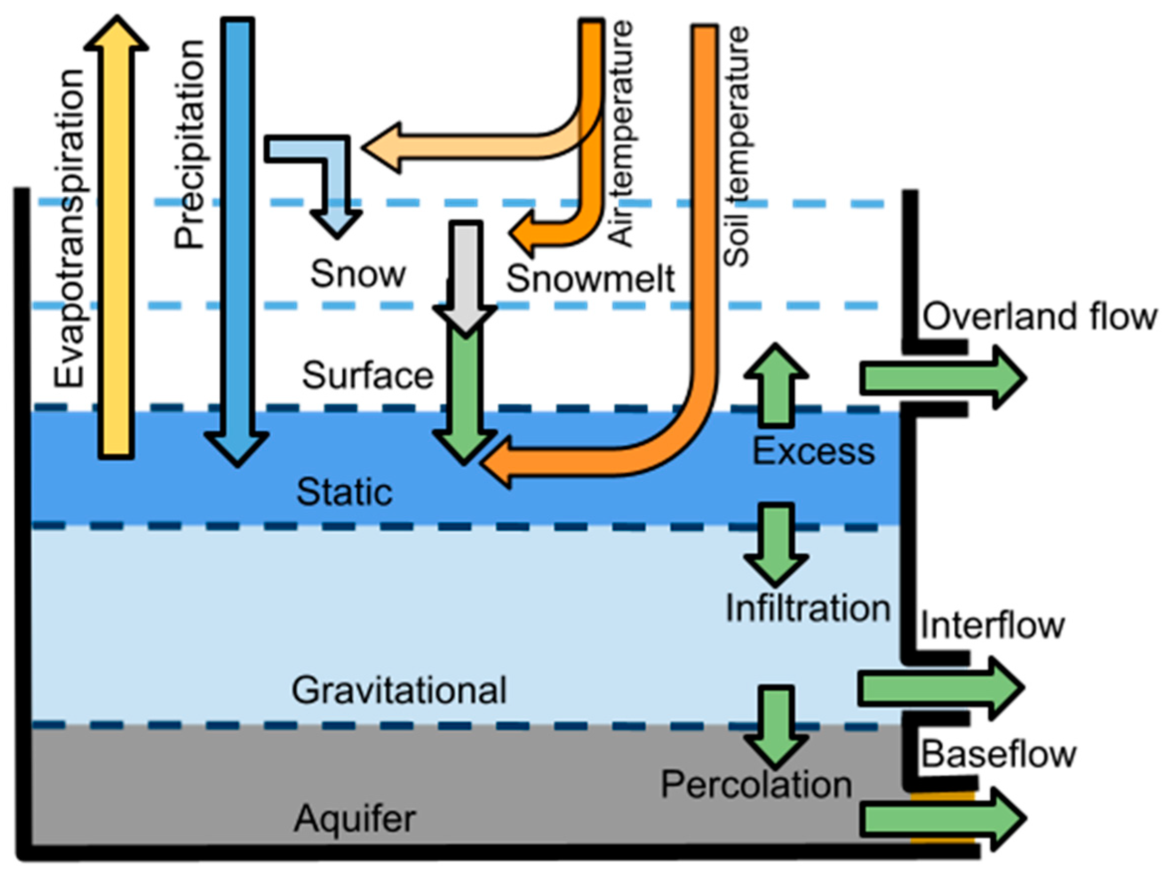
A schematic of the model is shown in Figure 1. The model uses six tanks to represent water storages in an extended soil column and the river. The tanks are called snow, static, surface, gravitational, aquifer, and channel. The vertical connections between tanks are the fluxes of precipitation, snowmelt, evapotranspiration, infiltration, and percolation. The horizontal outputs from the tanks represent the overland flow, interflow, base flow, and total discharge. The processes at each tank are described next.
2.3.1. Snow Tank
This storage represents the snow water equivalent H0, stored in the snowpack. We used the temperature threshold index (TI) method to simulate snow accumulation [17] and the degree-day method for snowmelt [18]. Precipitation X0 is added as snow to this tank if the air temperature is below a threshold value Tmax; otherwise, X0 is considered rainfall, X1. The air temperature threshold Tmax is a model parameter. Snowmelt Y0 is estimated using the melting rate parameter M and the temperature by:
Y0 = max (M T H0, H0)
If the frozen ground forcing indicates frozen conditions, the snowmelt and the rainfall skip the static tank and go as input to the surface tank. If the ground is not frozen, the snowmelt goes as input to the static tank. The mass balance equation for the snow tank is
2.3.2. Static Tank
This storage represents the initial abstractions H1 (interception and water detention in puddles) and the capillary water storage in the upper part of the soil. The capillary water storage is the water retained in the soil rooting zone by capillary forces and is a function of the field capacity and effective root depth. The static tank maximum storage Hmax is the sum of the maximum field capacity and effective root depth. Water exits the static tank only by evapotranspiration Y1 without contributing to the runoff. The inputs to the static tank when the ground is not frozen are the rainfall and the snowmelt. These are stored in the static tank until its maximum capacity Hmax is reached. The static exceedance X2 is defined as:
which is equivalent to assuming an infinite infiltration capacity until the static tank is filled.
X2 = max (0, X1 + Y0 − Hmax + H1)
The mass balance equation of the static storage is given by:
2.3.3. Surface Tank
This storage represents the water on the hillslope surface H2, which can either flow over the surface as surface runoff or infiltrate. The velocity of flow in the surface Vsurf is a model parameter and can be estimated based on the surface’s terrain slope and flow resistance. The amount of water that goes to the gravitational tank X3 is a function of the static storage exceedance X2 and an upper soil infiltration parameter I2:
X3 = min (X2, I2)
The upper soil infiltration can be derived from the upper soil saturated hydraulic conductivity Ks multiplied by the model temporal resolution Δt as I2 = Δt Ks. Therefore, X3 plus the flow derived to the static tank represents the total runoff abstractions. The overland flow at each hillslope is obtained with a linear reservoir approach as a function of overland flow velocity Vsurf and the width of the hillslope, which is approximated by L/Ah where L and Ah are the channel length and area of the hillslope, respectively
Y2 = Vsurf (L/Ah) H2
The mass balance for the surface storage is given by:
2.3.4. Gravitational Tank
This storage represents the gravitational storage in the upper part of the soil H3 between field capacity and saturation. The outflows of this tank are the deep percolation X4 and the hillslope interflow Y3. The percolated water X4 is a function of X3, and the infiltration rate of the deep soil I3. X4 is estimated by
X4 = min (X3, I3)
I3 can be estimated from the saturated hydraulic conductivity of the upper soil substratum Kp (deep soil or base rock) as I3 = Δt Kp. Interflow Y3 is obtained using a linear reservoir function as:
Y3 = C3 H3
The C3 residence time parameter is a function of the horizontal hydraulic conductivity of the upper part of the soil, which is mainly defined by its macropore structure. The mass balance for the gravitational storage is given by:
2.3.5. Aquifer
This storage represents the water stored in the lower layer of soil H4 before the bedrock. The outflows from this storage correspond to the groundwater outflow X5 and the base flow Y4. Groundwater outflow X5 represents the saturated flow that does not reach the surface catchment outlet; in this model implementation, the groundwater outflow is assumed to be zero. Base flow Y4 is calculated using a linear reservoir with a discharge coefficient C4 that can be related to the aquifer saturated hydraulic conductivity Kb using the equation:
Y4 = C4 H4
The mass balance for the aquifer storage is given by:
2.3.6. Channel
The sum of overland flow Y2, interflow Y3, and baseflow Y4 goes to the channel storage, representing the water stored in the channels of the river network. The equation describing the mass balance in the channel is given by:
where is a channel flow velocity parameter; is the channel link length; ExpQ and ExpA are parameters associated with the nonlinearity of flow velocity as a function of discharge in the channel and drainage area , respectively; is the area of the hillslope; and is the total discharge entering the channel from upstream. The terms and are constant unitary terms to keep the equation units consistent. Table 1 summarizes the model parameters and their units.
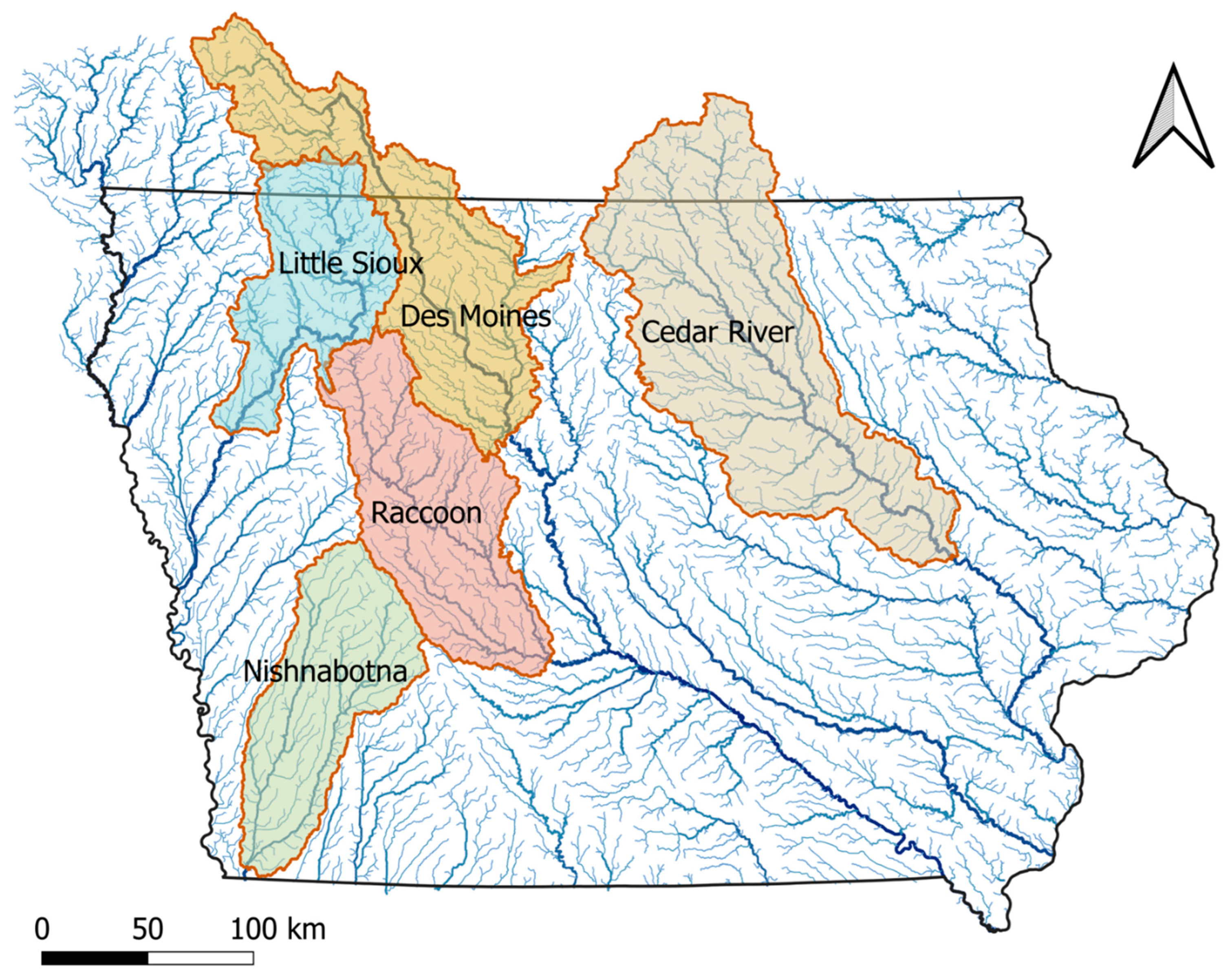
2.4. Study Area
We present applications of the new model in basins of Iowa. The basin locations are shown in Figure 2. The Cedar River basin at Cedar Rapids is located in Eastern Iowa. The basin has an area of 16,300 km2. The basin is predominantly devoted to agriculture of corn and soybean, with some urban developments in the lower part of the basin. The city of Cedar Rapids is the headquarters of diverse industries in the state. Flood level defined by the National Weather Service for this gage is reached at 900 m3s−1. The basin of the Des Moines River at Fort Dodge is located in north central Iowa, in the Des Moines Lobe landform. The basin has a drainage area of 10,830 km2. The land use is predominantly devoted to agriculture. The flood level defined by the National Weather Service for this gage is reached at 470 m3s−1. The Raccoon River basin at Van Meter is also in the Des Moines Lobe, with a drainage area of 8800 km2. The basin is also predominantly used for agriculture, has very flat slope, and their water used to supply water to the city of Des Moines. The flood level defined by the National Weather Service for this gage is reached at 650 m3s−1. The Little Sioux River at Correctionville is located in western Iowa, and it has a drainage area of 6450 km2. Land use is mostly agricultural, and it has steep hills. Flood level defined by the National Weather Service for this gage is reached at 380 m3s−1. In addition, in western Iowa, we selected the Nishnabotna River basin at Hamburg, with a drainage area of 7230 km2. The basin also has steep hills and man-made channels. Flood level defined by the National Weather Service for this gage is reached at 545 m3s−1.
3. Applications
In this section, we show some model applications, focusing on the aspects where previous model structures implemented in HLM had deficiencies. We present three applications: (1) a flood event where snow processes play an essential role, (2) simulations of discharge at the Des Moines Lobe landform, and (3) simulation of discharge at Western Iowa.
3.1. Simulation of Snow-Related Processes
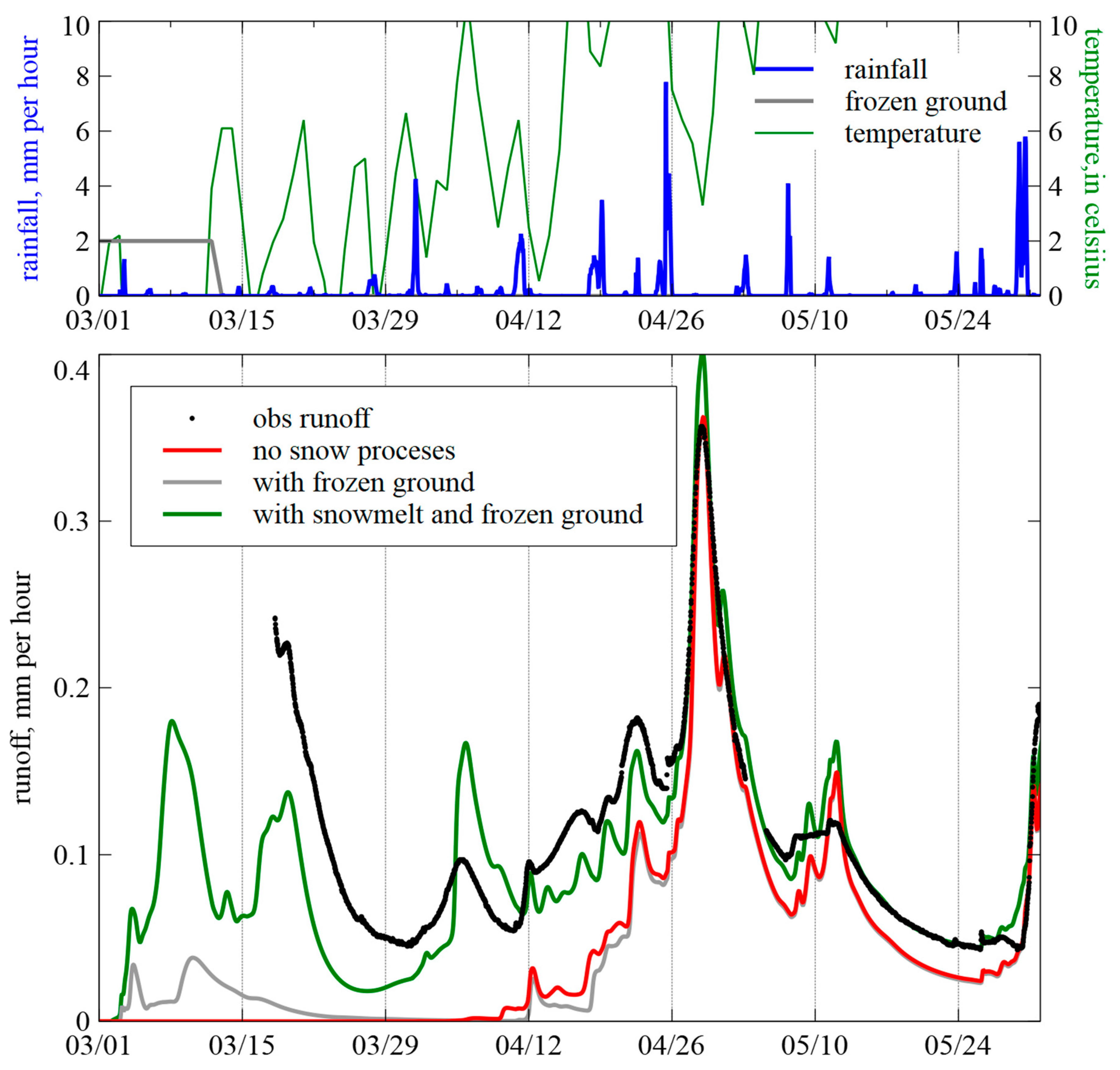
In June 2008, many watersheds in Iowa, including the Cedar River basin, experienced record floods. The genesis of the flood event is well described in [19,20,21]. During the cold season between 2007 and 2008, the Cedar River basin experienced a winter with heavy snow with water equivalent accumulations up to 100 mm in early March 2008 (SNODAS, https://nsidc.org/data/g02158, accessed on 1 July 2022). The upper panel of Figure 3 shows basin average hourly rainfall in blue based on Stage IV data; the green line shows the daily average air temperature according to gage data from the Mesonet network [22]. The black line in the bottom panel of Figure 3 shows the discharge observed at the United States Geological Survey gage in Cedar Rapids. The snow accumulation and melting were not directly responsible for the peak event of June. However, they left the soil saturated and triggered discharge events during March and April, which we analyze here. Temperatures above freezing point during March caused melting of the snowpack, leading to the discharge event observed on March 15. Unfortunately, discharge data before 15 March 2008 are not available at the gage, limiting tracking the evolution of the event.
The simulation of the hydrologic model with a configuration that does not include snow components is shown in red in the bottom panel of Figure 3. Without the snow processes, the model underestimates the runoff and cannot correctly simulate the discharge event between 15 March and 1 May, because forcing the model only with rainfall does not produce enough runoff volume to mimic the observed conditions. The gray line in the bottom panel of Figure 3 shows a configuration that does not accumulate or melt snow but considers if the ground is frozen and converts the rainfall into surface runoff. With this configuration, the observed frozen ground conditions during the first week of March (see the gray line in the upper panel of Figure 3) cause the rainfall of early March to become converted into surface runoff. A third model configuration is shown in green, where precipitation accumulates snow if temperatures are below 0 Celsius degrees, and the accumulated snowpack is melted at a rate of 5 mm day-1 Celsius degree-1. The snow storage is initialized with the values observed in the SNODAS data. With this configuration, the snow storage water helps the model reproduce better the discharge behavior in March and April. More accurate runoff estimation leads to reproducing better the falling limb of the hydrograph in late May. Including snow processes also sets the soil conditions that led to the event of June 2008
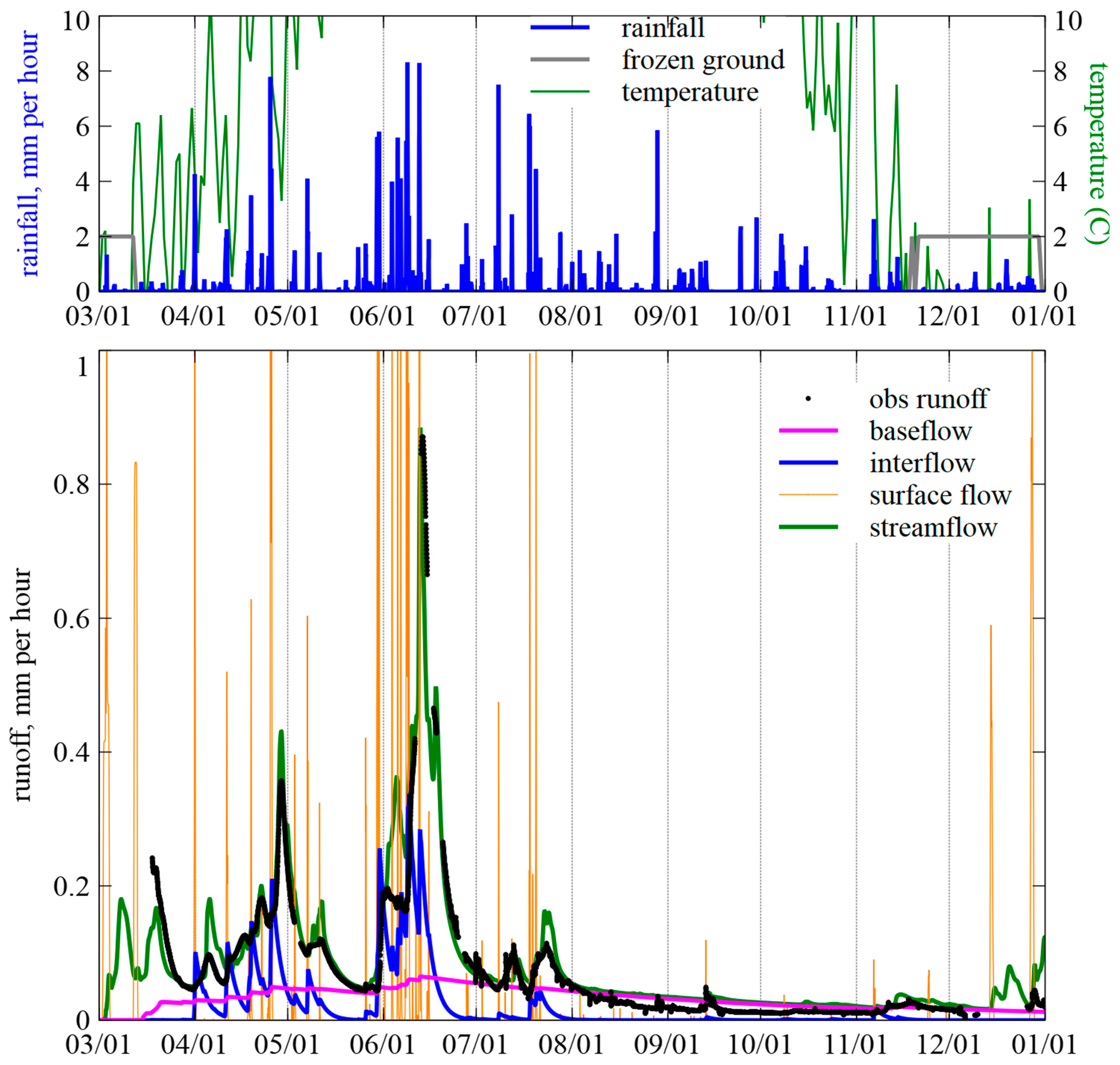
Now, we focus on the event of June 2008 in Figure 4. In late May, several storms trailed over Iowa, with rainfall falling over the saturated ground. The conditions were worsened by heavy rainfall across the Cedar River basin during 6–12 June. The observed peak reached 3900 m3s−1 on 15 June, producing the highest flow crest ever recorded in Cedar Rapids. Figure 4 shows observed and simulated flows in mm/hour to better understand how rainfall is transformed into different runoff components. The model streamflow simulation (shown in green) accurately reproduces the observed flood event. We show the decomposition of streamflow into the surface flow (in orange), interflow (in blue) and base flow (in purple) components. It is important to keep track of the magnitude of each one of those flow components, because there are model parameter sets that can lead to streamflow simulations similar to the one presented here but created from an inadequate proportion of the flow components. In this case, the baseflow coincides with the minimum values observed between hydrographs. The interflow concurs with the recessions and explains a significant portion of the volume. Moreover, the surface flows coincide with the observed peaks. The described decomposition is a numerical estimation of the fluxes involved that highlights the relevance of each process. The model reproduces adequately the falling limb of the hydrograph between the 15 June peak and 1 July. There is some overestimation of the baseflow conditions between August 1 and the end of the year.
We checked the mass conservation during the time period shown in Figure 4 for the precipitation input and flow components. The basin total rainfall accumulation is 1021 mm; total runoff is 596 mm; total overland flow is 222 mm, which is 37% of total runoff; total interflow is 141 mm, which is 23% of total runoff; and total baseflow is 233 mm, which is 39% of total runoff. There are 15 mm of water that remain stored in the soil at the end of the time period.
3.2. Simulation of discharge at the Des Moines Lobe and Western Iowa
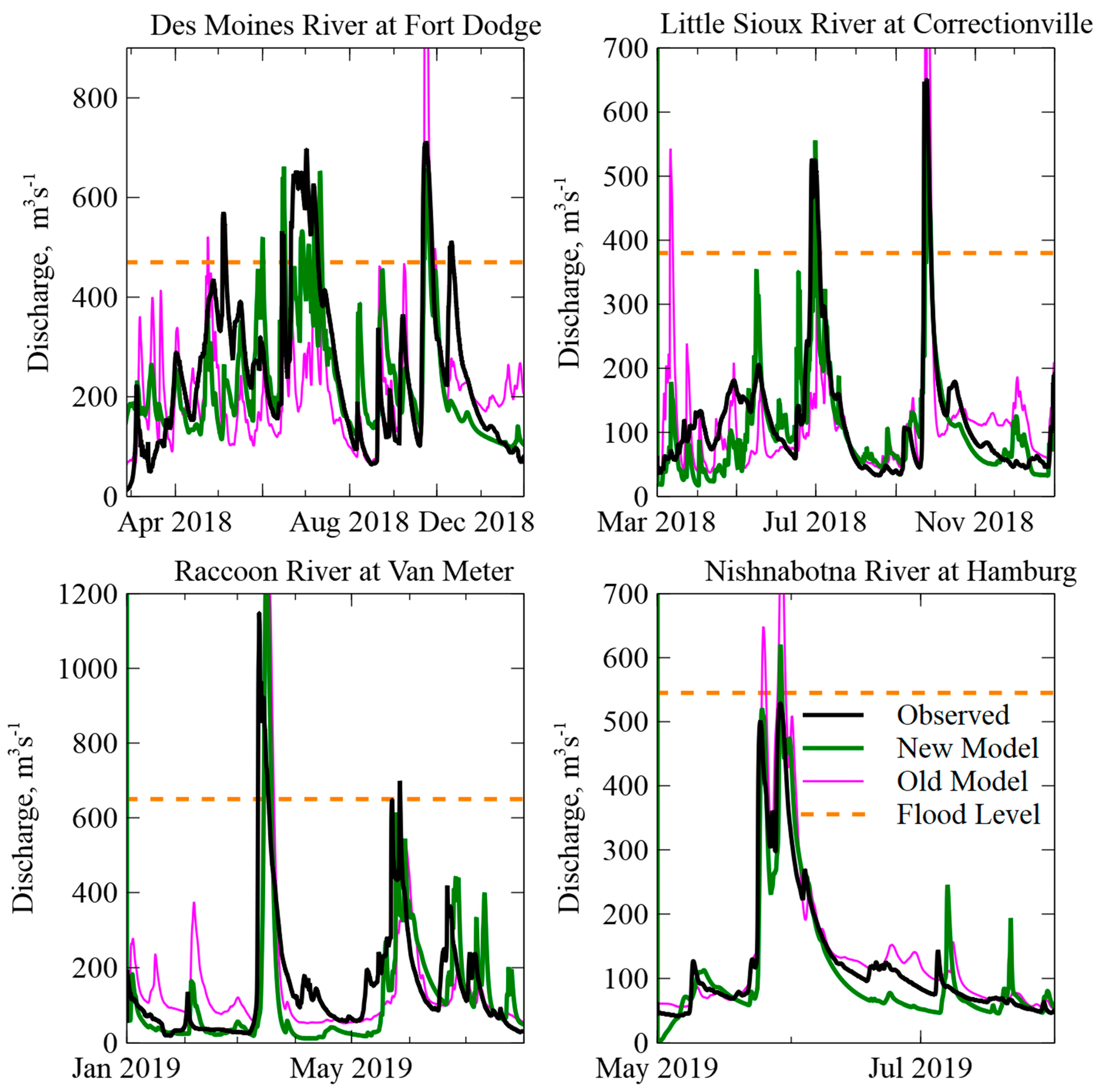
Figure 5 presents streamflow simulations at basins in the Des Moines Lobe and Western Iowa. In this area, previous model developments had challenges reproducing the hydrologic response [11,14]. The upper left panel shows the results at the Des Moines River basin at Fort Dodge, which is located in the Des Moines Lobe. Simulations from previous model structures (in purple) in this basin could not represent the discharge volumes in May and June due to the lack of accounting for snowmelting, poor replication of the falling limb, and recession of the hydrographs. With the new model structure (in green), there is an improvement representing the falling limbs and the recession during the last part of the year. Some issues in the rainfall input limited the accounting for better volume estimation in May and one event in December.
The bottom left panel shows the results of the Raccoon River basin at Van Meter, which is also located in the Des Moines Lobe. Simulations from previous model structures in this basin were characterized by having a poor replication of the falling limb and recession of the hydrographs. The new simulations capture well the peak flow and have better recessions. There was a limitation in capturing the discharge volume in May 2019 due to issues estimating snow water equivalent from the precipitation product.
The upper right panel shows the results at the Little Sioux River basin at Correctionville, which is located in Western Iowa. Compared to simulations from the old model where there were problems in estimating volume in the summer months, the new model structure produces a reasonable estimation of the volume and the recession of the flows. The lower right panel shows results at the Nishnabotna River basin in Hamburg, which is located in Western Iowa. The figures show a flow event in June 2019 where the model captures the rising and falling limbs of the hydrographs, as well as the observed double peak structure and their magnitude, better than the old model structure.
4. Conclusions
This paper introduced a new model structure compatible with the Hillslope Link Model framework. The model structure was designed to overcome some limitations of the previous models, including the lack of snow modeling components and giving more flexibility to the infiltration and overland flow processes, which were tightly coupled in previous model structures. The proposed model structure still has some limitations and does not reproduce perfectly every characteristic of runoff generation and routing. However, the contribution of this new model is gaining in flexibility, and the model structure allows for better characterization of the runoff generation processes and relating the model parameters with the soil hydraulic properties and features of the landscape. Suggested improvements for the new model will be derived from subsequent research ongoing by the authors, which explores the performance of the proposed model in more basins and over a longer period of study.
Author Contributions
All authors contributed equally to the paper. All authors have read and agreed to the published version of the manuscript.
Funding
Both authors are funded by the Iowa Flood. Felipe Quintero received funding from Iowa Department of Transportation (Project number 20-SPR2-002). Nicolas Velasquez received funding from Mid-America Transportation Center via a grant from the U.S. Department of Transportation’s University Transportation Centers Program (USDOT UTC grant number for MATC: 69A3551747107), the Iowa Highway Research Board and Iowa Department of Transportation (Contract number:TR-699).
Acknowledgments
The authors would like to acknowledge the Iowa Flood Center, Iowa Department of Transportation, and Mid-America Transportation Center for their support.
Conflicts of Interest
The authors declare no conflict of interest.
References
- Centre for Research on the Epidemiology of Disasters Crunch 66-Disasters Year in Review 2021. Available online: https://cred.be/sites/default/files/CREDCrunch66N.pdf (accessed on 10 May 2022).
- Chatzichristaki, C.; Stefanidis, S.; Stefanidis, P.; Stathis, D. Analysis of the flash flood in rhodes island (south Greece) on 22 November 2013. Silva Balc. 2015, 16, 76–86. [Google Scholar]
- Diakakis, M. Characteristics of Infrastructure and Surrounding Geo-Environmental Circumstances Involved in Fatal Incidents Caused by Flash Flooding: Evidence from Greece. Water 2022, 14, 746. [Google Scholar] [CrossRef]
- Porter, J.R.; Shu, E.; Amodeo, M.; Hsieh, H.; Chu, Z.; Freeman, N. Community flood impacts and infrastructure: Examining national flood impacts using a high precision assessment tool in the united states. Water 2021, 13, 3125. [Google Scholar] [CrossRef]
- Mantilla, R.; Krajewski, W.F.; Velasquez, N.; Small, S.J.; Ayalew, T.B.; Quintero, F.; Jadidoleslam, N.; Fonley, M. The Hydrological Hillslope-Link Model for Space-Time Prediction of Streamflow: Insights and Applications at the Iowa Flood Center. In Extreme Weather Forecasting; Astitha, M., Nikolopoulos, E.I., Eds.; Elsevier: Amsterdam, The Netherlands, 2022; ISBN 9780128201244. [Google Scholar]
- Quintero, F.; Krajewski, W.F.; Mantilla, R.; Small, S.; Seo, B.-C. A Spatial–Dynamical Framework for Evaluation of Satellite Rainfall Products for Flood Prediction. J. Hydrometeorol. 2016, 17, 2137–2154. [Google Scholar] [CrossRef]
- Krajewski, W.F.; Ceynar, D.; Demir, I.; Goska, R.; Kruger, A.; Langel, C.; Mantilllla, R.; Niemeier, J.; Quintero, F.; Seo, B.C.; et al. Real-time flood forecasting and information system for the state of Iowa. Bull. Am. Meteorol. Soc. 2017, 98, 539–554. [Google Scholar] [CrossRef]
- Fonley, M.R.; Qiu, K.; Velásquez, N.; Haut, N.K.; Mantilla, R. Development and Evaluation of an ODE representation of 3D subsurface tile drainage flow using the HLM flood forecasting system. Water Resour. Res. 2021, 57, e2020WR028177. [Google Scholar] [CrossRef]
- Ayalew, T.B.; Krajewski, W.F.; Mantilla, R.; Small, S.J. Exploring the effects of hillslope-channel link dynamics and excess rainfall properties on the scaling structure of peak-discharge. Adv. Water Resour. 2014, 64, 9–20. [Google Scholar] [CrossRef]
- Quintero, F.; Krajewski, W.F.; Seo, B.C.; Mantilla, R. Improvement and evaluation of the Iowa Flood Center Hillslope Link Model (HLM) by calibration-free approach. J. Hydrol. 2020, 584, 124686. [Google Scholar] [CrossRef]
- Lin, Y.; Mitchell, K.E. The NCEP Stage II/IV hourly precipitation analyses: Development and applications. In Proceedings of the 19th Conference on Hydrology, American Meteorological Society, San Diego, CA, USA, 9–13 January 2005; Paper 1.2. pp. 2–5. [Google Scholar]
- Seo, B.-C.; Krajewski, W.F. Statewide real-time quantitative precipitation estimation using weather radar and NWP model analysis: Algorithm description and product evaluation. Environ. Model. Softw. 2020, 132, 104791. [Google Scholar] [CrossRef]
- Velásquez, N.; Mantilla, R.; Krajewski, W.; Fonley, M.; Quintero, F. Improving Hillslope Link Model Performance from Non-Linear Representation of Natural and Artificially Drained Subsurface Flows. Hydrology 2021, 8, 187. [Google Scholar] [CrossRef]
- Vélez, J.I. Estrategia de simulación hidrológica distribuida: Integración conceptual de hidrología, hidráulica y geomorfología. Rev. Acad. Colomb. Cienc. Exactas Físicas Nat. 2013, 37, 393–409. [Google Scholar]
- Francés, F.; Vélez, J.I.; Vélez, J.J. Split-parameter structure for the automatic calibration of distributed hydrological models. J. Hydrol. 2007, 332, 226–240. [Google Scholar] [CrossRef]
- Small, S.J.; Jay, L.O.; Mantilla, R.; Curtu, R.; Cunha, L.K.; Fonley, M.; Krajewski, W.F. An asynchronous solver for systems of ODEs linked by a directed tree structure. Adv. Water Resour. 2013, 53, 23–32. [Google Scholar] [CrossRef]
- Singh, V.P. The Snowmelt Runoff Model (SRM). Comput. Model. Watershed Hydrol. 1995, 1, 477–520. [Google Scholar]
- Martinec, J.; Rango, A. Areal distribution of snow water equivalent evaluated by snow cover monitoring. Water Resour. Res. 1981, 17, 1480–1488. [Google Scholar] [CrossRef]
- Budikova, D.; Coleman, J.S.M.; Strope, S.A.; Austin, A. Hydroclimatology of the 2008 Midwest floods. Water Resour. Res. 2010, 46, W12524. [Google Scholar] [CrossRef] [Green Version]
- Krajewski, W.F.; Mantilla, R. Why Were the 2008 Floods So Large? In A Watershed Year: Anatomy of the Iowa Floods of 2008; University of Iowa Press: Iowa City, IA, USA, 2010; p. 9. [Google Scholar]
- Mutel, C.F. A Watershed Year: Anatomy of the Iowa Floods of 2008; University of Iowa Press: Iowa City, IA, USA, 2010. [Google Scholar]
- Todey, D.P.; Herzmann, D.E.; Takle, E.S. The Iowa Environmental Mesonetcombining observing systems into a single network. In Sixth Symposium on Integrated Observing Systems; Iowa State University: Ames, IA, USA, 2002. [Google Scholar]
Figure 1.
Schematics of the TETIS model structure in HLM.

Figure 2.
Basins selected to evaluate the model implementation.

Figure 3.
Model simulation in Cedar River at Cedar Rapids, from 1 March to 1 June 2008. The upper panel shows basin average rainfall and temperature. The gray line indicates when ground is frozen. The bottom panel shows streamflow simulations with and without snow components.
Figure 3.
Model simulation in Cedar River at Cedar Rapids, from 1 March to 1 June 2008. The upper panel shows basin average rainfall and temperature. The gray line indicates when ground is frozen. The bottom panel shows streamflow simulations with and without snow components.

Figure 4.
Model simulation in Cedar River at Cedar Rapids from 1 March 2008 to 1 January 2009. The upper panel shows basin average rainfall and temperature. The gray line indicates when ground is frozen. Bottom panel shows the decomposition of streamflow simulations into surface flow, interflow and baseflow.

Figure 5.
Flow simulations obtained at basins of the Des Moines Lobe landform (left column) and basins in Western Iowa.
Figure 5.
Flow simulations obtained at basins of the Des Moines Lobe landform (left column) and basins in Western Iowa.


Table 1.
Model parameter names, symbols and units required in HLM.
| Name | Symbol | Units Required |
|---|---|---|
| Air temperature threshold | Tmax | Celsius degree |
| Melting rate | M | mm/day/degree Celsius |
| Maximum storage static tank | Hmax | mm |
| Upper soil infiltration rate | I2 | mm/hour |
| Overland flow velocity | Vsurf | m/s |
| Deep soil infiltration rate | I3 | mm/hour |
| Gravitational storage residence time | C3 | Days |
| Aquifer storage residence time | C4 | Days |
| Flow velocity in channel | Vc | m/s |
| Discharge exponent | ExpQ | Adimensional |
| Drainage Area exponent | ExpA | Adimensional |
Publisher’s Note: MDPI stays neutral with regard to jurisdictional claims in published maps and institutional affiliations. |
© 2022 by the authors. Licensee MDPI, Basel, Switzerland. This article is an open access article distributed under the terms and conditions of the Creative Commons Attribution (CC BY) license (https://creativecommons.org/licenses/by/4.0/).
Share and Cite
MDPI and ACS Style
Quintero, F.; Velásquez, N. Implementation of TETIS Hydrologic Model into the Hillslope Link Model Framework. Water 2022, 14, 2610. https://doi.org/10.3390/w14172610
AMA Style
Quintero F, Velásquez N. Implementation of TETIS Hydrologic Model into the Hillslope Link Model Framework. Water. 2022; 14(17):2610. https://doi.org/10.3390/w14172610
Chicago/Turabian StyleQuintero, Felipe, and Nicolás Velásquez. 2022. "Implementation of TETIS Hydrologic Model into the Hillslope Link Model Framework" Water 14, no. 17: 2610. https://doi.org/10.3390/w14172610
Note that from the first issue of 2016, this journal uses article numbers instead of page numbers. See further details here.