
Flushing Capacity of a Stored Volume of Water: An Experimental Study


1
Hidr@m Research Group, Department of Mining and Civil Engineering, Universidad Politécnica de Cartagena, 30203 Cartagena, Spain
2
Department of Civil and Environmental Engineering, Escuela Politécnica Nacional, Quito 170143, Ecuador
*
Author to whom correspondence should be addressed.
Water 2022, 14(17), 2607; https://doi.org/10.3390/w14172607
Submission received: 24 July 2022
/
Revised: 17 August 2022
/
Accepted: 19 August 2022
/
Published: 24 August 2022
(This article belongs to the Special Issue Hydraulic, Sediment Transport and Morphological Assessment in Rivers and Reservoirs)
Abstract
:This paper presents a systematic analysis of the hydraulic flushing capacity of a stored volume of water to remove sediments. This analysis is based on 90 laboratory experiments in which the volume of sediment evacuated was measured for varying initial volumes of water, three bed slopes, and three sediment sizes. The experiments consisted of the rapid emptying of a reservoir by means of suddenly opening a tilting gate downstream. This opening produced an accelerated flow which eroded the mobile bed of the reservoir. The efficacy of flushing, herein defined as the ratio of the volume of sediments evacuated to the volume of water released, increased with the initial slope, and decreased as the initial volume of water increased. In relation to the sediment size, while the results obtained for the coarse and medium sands were very similar to each other, the results obtained for the fine sand were affected by the existence of apparent cohesion in the mobile bed. In comparison to the results obtained for the medium and coarse sands, this apparent cohesion reduced the volume of sediment evacuated by a given volume of water and hence, the efficacy of flushing.
1. Introduction
Reservoir sedimentation has become a major concern for dams’ operators and owners. The gradual and incessant loss of storage capacity in reservoirs, owing to sediment deposition, reduces their operability and sustainability. In addition, the impoundment of sediments upstream of the dam alters the riverine sediment balance, resulting in a lack of sediments downstream [1,2]. This, in turn, leads to bed erosion and impoverished habitats downstream, owing to a deficit in those nutrients transported with the sediment particles [1,3]. In addition, the dam impedes the natural migration of riverine species upstream, which often results in a reduction in the species richness and the number of some assemblages [4]. In extreme cases, the sediment deposits in reservoirs may partially or totally block the water release structures, or even render the reservoir definitively inoperable [5,6]. The worldwide average loss of storage capacity has been estimated to range from 0.5% to 1.0% of volume per year [2,6,7,8]. Nevertheless, and depending on the region, this rate may reach higher values, such as the 4.3% reported by [9] for the reservoirs of California State in 2008. At a global scale, the loss of storage capacity owing to reservoir sedimentation, and the decrease in the rate at which new reservoirs are being built, have led to a decrease in the total net reservoir storage volume since 2000, and a decrease in the storage volume per capita since 1980 [1]. Moreover, these trends may be aggravated by a climate change scenario in which sediment yield is expected to increase [10,11], thereby raising the amounts of sediment being deposited in reservoirs.
Sediment management strategies seek to mitigate the negative effects derived from sediment depositing in reservoirs. Such strategies can be classified into three groups: (i) measures to reduce the fraction of sediment yield that enters the reservoirs; (ii) measures to minimize sediment deposition within reservoirs; and (iii) measures to recover or to increase storage volume in the reservoir [2,12,13]. Among the measures included in the third group, the present study focuses on hydraulic flushing, which consists of the opening of the low-level outlets of a dam to remove previously deposited sediments. In addition, extreme cases of flushing are those dam removal projects in which the reservoirs are rapidly drawn down by breaching the dam [14,15,16]. Flushing has been reported as being one of the most efficient techniques for removing sediments from a reservoir [2,17,18]. However, this efficiency depends on factors such as the initial water level, the geometry of the reservoir, the capacity of the low-level outlets, the hydrology of the region, and the characteristics of the sediment deposited. Thus, when flushing is carried out with a water level that is so high as to cause a pressure flow through the low-level outlets, it is called pressure flushing, and the resulting erosion is limited to a cone-shaped zone in the vicinity of the outlets [19]. On the contrary, when the water level drops and the flow becomes a free-surface flow, it is called free-flow flushing, and the resulting erosion may extend several kilometers upstream of the outlets, eroding a channel and removing a large volume of sediments from the reservoir. Those reservoirs equipped with low-level outlets with a relatively large capacity, located in narrow valleys with steep sides, steep longitudinal slopes, and with strong seasonal flow patterns are the most suitable for successful flushing [2,13,17]. Additionally, [12] stated that, for flushing to be successful, the ratio of capacity to mean annual flow of the reservoir should be less than 4%, because a larger capacity would affect the reservoir draw down. Furthermore, periodic and controlled release of sediments from a reservoir can be beneficial for the riverine ecosystem, as it reduces the deficit of sediments downstream of the dam and may provide spawning grounds for fishes, especially when gravel predominates among the released sediments. On the contrary, when fine sediments are predominant in the release, severe environmental impacts can be created downstream of the dam. Flushing releases with fine sediments are characterized by high sediment concentrations and, consequently, they reduce the oxygen concentration, the visibility, and the light penetration. The deposition of sediment also often results in infilled pools and bed clogging, reducing the sites for spawning and impoverishing fish habitats [1].
The existing knowledge about flushing has been gained mainly from case studies based on field observations and measurements, performed during flushing operations in real reservoirs [2,3,13,17,18]. In addition, numerical studies, also based on case studies, have significantly contributed to characterizing and optimizing the processes involved in flushing [20,21,22,23]. In contrast, few experimental studies conducted under controlled laboratory conditions have systematically investigated the flushing technique. This is the case of the studies by [14], which focused on the geomorphic response of a channel after a dam removal, and that by [24], which focused on the evolution and characterization of the flushing channel and on the amount of sediment removed. Furthermore, in most of the flushing operations documented by the studies referred to above, sediments were eroded by the natural discharge of the river, which flowed through the low-level outlets as a free-surface flow. In this context, the present study focuses on those reservoirs located in arid or semiarid regions in which the hydrological conditions result in weak river discharges with low or negligible erosion capacity for flushing. Thus, the available water for flushing is that previously stored in the reservoir.
Therefore, the present study proposes a detailed, novel, and systematic experimental approach with the following objectives:
- To analyze the capacity of flushing sediments in a reservoir using only that water previously stored in it.
- To characterize the effects of the initial water head, the initial volume of water, the bed slope, and the sediment grain size on the efficacy of flushing. This efficacy is herein defined as the volume of sediments removed to the volume of water released.
To address these objectives, 90 laboratory experiments were conducted at the hydraulic laboratory of Universidad Politécnica de Cartagena, Spain. These experiments included different configurations of the reservoir geometry, bed slope, and sediment grain size.
2. Methodology
2.1. Experimental Facility and Procedure
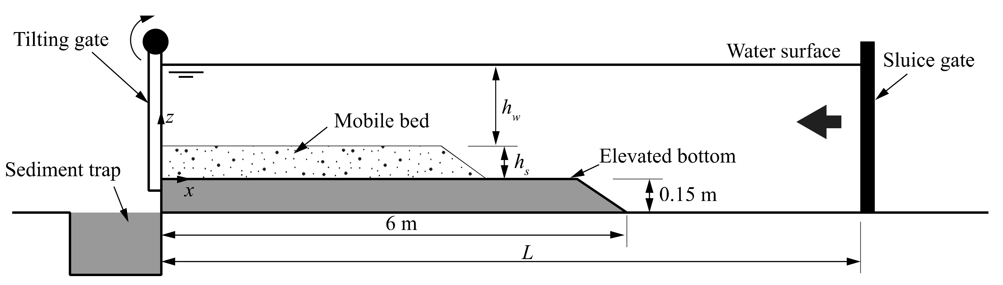
The experimental facility consisted of a 15 m long, 0.31 m wide, and 0.50 m high rectangular glass-wall flume, with an adjustable longitudinal slope. The flume was equipped with a sluice gate upstream, a tilting gate downstream, and a sediment trap at the downstream end of the flume. The tilting gate was the same width as the flume (B = 0.31 m) to characterize the maximum hydraulic capacity of the stored volume for flushing. The bottom was elevated 0.15 m along 6 m, to ensure supercritical flow downstream of the tilting gate. The origin of coordinates was located at the downstream end on the elevated bottom (Figure 1).
Figure 1 sketches a lateral view of the experimental facility in which hs stands for the initial thickness of the sediment layer, hw is the initial water head measured from the top of the sediment layer, and L is the reservoir length, comprised between the tilting gate (downstream) and the sluice gate (upstream) (Figure 1). Both hw and hs varied from 0.05 m to 0.20 m by intervals of 0.05 m, and combined they gave ten pairs hs—hw, in which:
- For hs = 0.05 m, hw = 0.05 m, 0.10 m, 0.15 m, and 0.20 m.
- For hs = 0.10 m, hw = 0.05 m, 0.10 m, and 0.15 m.
- For hs = 0.15 m, hw = 0.05 m, and 0.10 m.
- For hs = 0.20 m, hw = 0.05 m.
The sediments consisted of three non-cohesive, well-sorted silica-sands (ρs = 2600 kg/m3) with d50 = 0.39, 0.80, and 1.54 mm, referred to as fine, medium, and coarse, respectively.
The experimental set-up consisted of a total of 90 experiments, including:
- Thirty experiments in which ten pairs hs—hw were tested for an initial bed slope S0 = 0.0%, for the medium sand, and for three different reservoir lengths: L = 5.997 m, 9.287 m, and 12.043 m with ΔL = ±0.001 m accuracy.
- Twenty experiments in which ten pairs hs—hw were tested for S0 = 0.5%, and 1.0%, for the medium sand, and for L = 12.043 m.
- Forty experiments in which ten pairs hs—hw were tested for S0 = 0.0%, for the fine and coarse sands, and for L = 5.997 m, and 12.043 m.
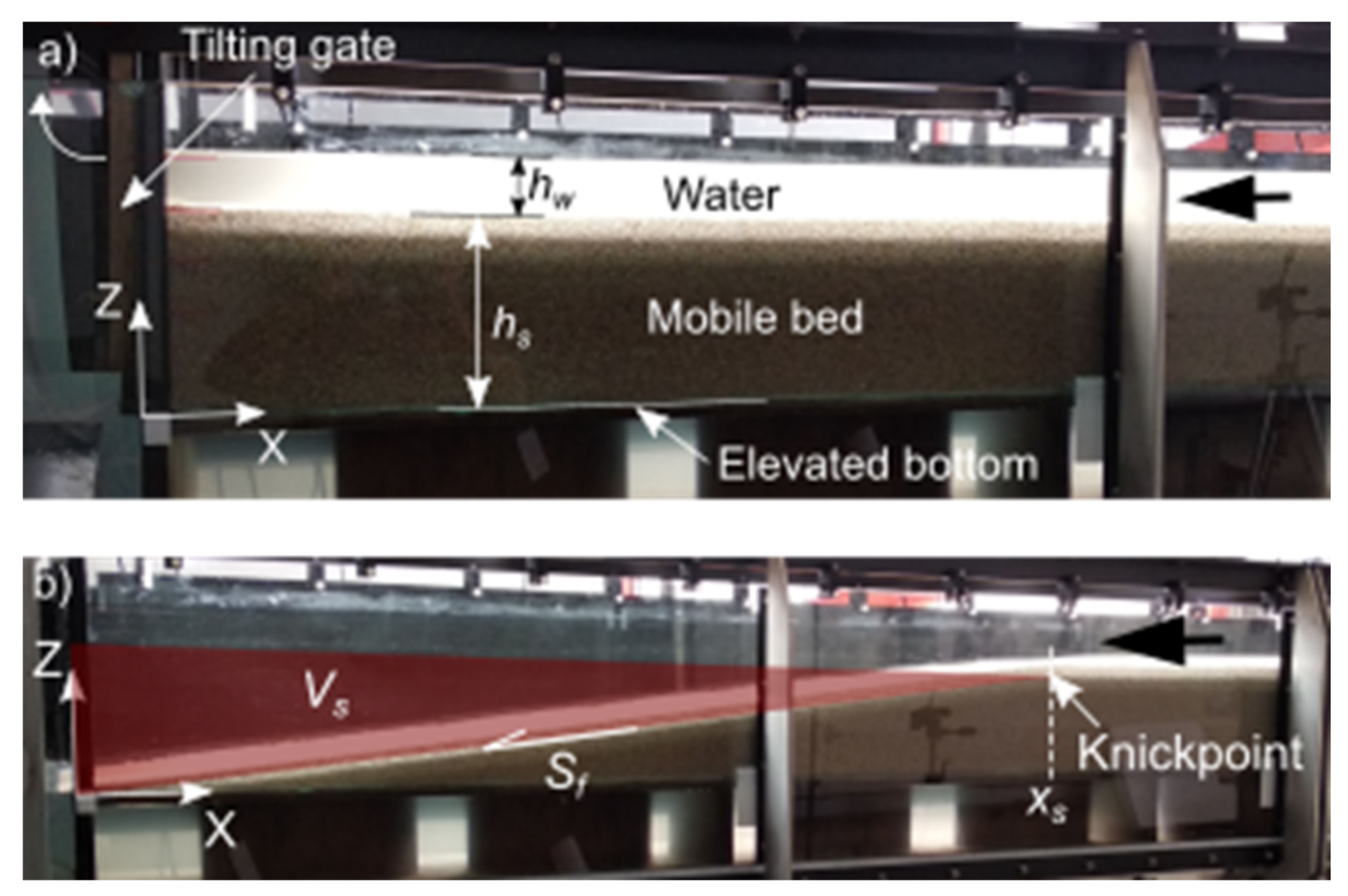
Prior to each experiment, a layer of unconsolidated loose sediments of thickness hs was extended and leveled throughout the elevated bottom with Δhs = ±0.003 m accuracy. Later, the flume was carefully filled up with water until reaching the level hw with Δhw = ±0.001 m accuracy, and the upstream sluice gate was closed to confine the initial volume of water (Vw). The experiment started with a sudden opening of the tilting gate, and it finished when the initial volume of water (Vw) was completely evacuated from the flume, along with a volume of sediments (Vs). These sediments were collected in the sediment trap, to be reused in subsequent experiments. Once the experiment had finished, the abscise of the final position of the knickpoint xs was measured with Δxs = ±0.005 m accuracy (Figure 2). All the experiments were laterally recorded to follow the evolution of the bed and the water surface. Figure 2 shows a lateral view of the experimental facility just before the beginning of one experiment and after finishing it. The final slope of the bed, downstream of the knickpoint, was computed as Sf = hs/xs (Figure 2b), and Vs was estimated geometrically as:
Thus, the steeper Sf, the lower Vs, and vice versa. The measurement errors of Sf and Vs were estimated as:
where ΔB = ±0.005 m.
2.2. Dimensional Analysis
A dimensional analysis was performed in order to characterize the effects of the reservoir geometry, the sediment characteristics, and the initial water head on Sf. Thus, Sf depends on the following variables:
where, obviating those variables already defined, B is the width of the flume, ρ is the density of water, υ is the kinematic viscosity of water, g is the gravitational acceleration, and u*_cr is the critical shear velocity according to [25]. In this analysis, B can be eliminated because it remains constant for all the experiments. Thus, by considering hs as the length scale, ρ·hs3 as the mass scale, and hs/u*_cr as the time scale, the Buskingham π theorem yields:
which, rearranged, reads:
which is equivalent to:
where Re* and τ*_cr are the Shields’ parameters [25]. These parameters can be combined as D* = Re*2/3 · τ*_cr1/3, which is the non-dimensional sediment diameter [26]. Thus, the dimensional analysis finally yields:
where hw·L/hs2 is the product of the initial water head to sediment thickness ratio (hw/hs) and the reservoir length to sediment thickness ratio (L/hs). The measurement error of the parameter hw·L/hs2 was estimated as:
This analysis is also valid for characterizing the flushing efficacy (Vs/Vw) as a function of the reservoir geometry, the sediment characteristics, and the initial water head. Thus, by expressing Sf as a function of Vs from Equation (1) and substituting in Equation (8), it reads:
where multiplying the term on the left side by hw/hs and by L/hs, and multiplying the first parameter on the right side by B/hs, it reads:
which is equivalent to:
where Vs/Vw stands for the efficacy of the flushing, and Vw/hs3 is the non-dimensional initial volume of water. Table 1 shows the values adopted in this study for the aforementioned governing parameters.
2.3. Studies for Comparison
The results obtained in this study have been compared to the results obtained from laboratory experiments by [24], and to the field measurements reported for the flushing operations of the Condit dam in USA [15], and the Gebidem dam in Switzerland [2]. Despite the existing differences between these previous studies and the experiments conducted in this study, mainly in terms of reservoir and outlet geometries and sediment characteristics, all these studies report on the rapid release of a previously stored volume of water, which provokes the erosion of the bed evacuating a volume of sediments. For comparison, the values of the variables L, hw, hs, Vw, Vs, and Sf were obtained for each of these previous studies, to compute the parameters hw·L/hs2 and Vw/hs3. The effects of S0 and D* on the final bed slope (Sf) and on the efficacy of flushing (Vs/Vw) were not analyzed for these studies, because the available data did not enable the individual effects of these variables on the overall process to be decoupled.
The experiments by [24] were conducted in a 50 m long, 2.4 m wide, horizontal and rectangular flume at the hydraulic laboratory of University of California at Berkeley (USA). In that flume, a reservoir was modeled within the upstream 30 m of the flume. The outlet consisted of a 0.15 m wide, 0.25 m high rectangular sluice gate, located at the downstream end of the reservoir. For each experiment, a 0.10 m thick and unconsolidated sediment layer was extended on an elevated bottom, approximately 9 m from the outlet. The sediment material consisted of walnut shell grit (d50 = 1.25 mm and ρs = 1.39 kg/m3). The reservoir was filled with water until the desired water level was reached. Then, the discharge was set to the desired value and the sluice gate was opened until the steady state was reached, i.e., constant water level and the outlet discharge equal to the incoming one. To start the experiments, the gate was opened at a constant rate of approximately 5 cm per minute, until the opening reached 10 cm above the elevated bottom. Each experiment lasted approximately 30 min, during which time the incoming discharge was kept constant, and the outlet hydrograph and solidograph were measured. In those experiments, different discharges ranging from 0.56 m3/s to 4.86 m3/s were tested. The initial water level (hw) varied from 0.02 m to 0.07 m, measured from the top of the sediment layer. The data for those experiments were obtained directly from [27], with the exception of L and Vw. L was estimated as Vw/(B·hw) for each run, where B was the width of the laboratory flume, i.e., 2.4 m, and Vw was computed from the corresponding liquid hydrograph.
The case of the Condit dam consisted of the removal of a 38 m-high dam on the White Salmon River (USA), which stored 1.8·106 m3 of sediments. Prior to the demolition of the dam, the reservoir was rapidly emptied by blasting a 5 m wide hole into the base of the dam. This blast led to a rapid reservoir draw down and to an abrupt release of water and sediments, which lasted approximately five hours [15]. During that time, a channel was eroded approximately 1 km from the dam. Although the erosion and the transport of sediment downstream of the dam continued for several weeks, it was provoked by the natural discharge of the river, rather than by the water previously stored in the reservoir. Hence, in this study, only the first five hours after breaching were considered for comparison. Thus, L, hw, hs, and Sf were obtained directly from Figure 2 in [15]. hs was estimated as the average difference between the pre-dam bathymetry and that performed in 2006, considering the nearest 1 km to the dam. Sf was estimated from the 56 days post-breach profile, by considering an average value for the nearest 1 km to the dam. Vs and Vw were calculated for the first five hours after the dam breaching from the sediment concentrations and discharge hydrograph, respectively (Figure 4 in [15]).
The third case considered for comparison in this study is that concerning the flushing operation conducted in the Gebidem dam in Switzerland, in 1991 [2]. This flushing operation began with the water level of the reservoir at its minimum operational level, at which the water surface extended some 450 m from the dam. Then, the low-level outlets were opened for 96 h, while the discharge hydrograph and suspended sediment concentrations were measured. The volume of water previously stored in the reservoir was released within the first two hours of flushing. After that, the natural river discharge flowed through the low-level outlets, carrying sediments downstream of the dam. In that study, only the first two hours of flushing were considered for comparison. In this case, L, hw, hs, and Sf were estimated from Figure 21.8 in [2], by considering the nearest 450 m to the dam. Vw and Vs were computed from the discharge hydrograph and the values of suspended solid concentrations shown in Figure 21.6 in [2]. Table 2 contains the values of the variables and parameters needed for comparison.
Other field and laboratory studies in which water and sediments were suddenly released by an abrupt dam removal were also analyzed for comparison, but they were discarded for different reasons. These are the cases of the removal of the Marmot dam [16], the failure of the Barlin dam [28], and the experiments by [14]. The case of the Marmot dam was discarded because the water stored in the reservoir prior to the dam breaching was mostly responsible for the erosion of the earth cofferdam, whereas the sediments impounded in the reservoir were mostly eroded by the natural discharge of the river. [16]. The abrupt failing of the Barlin dam in Japan during the typhoon WeiPa in 2007 was discarded for comparison, because no data of the volume of water previously stored in the reservoir were found [28]. The experiments by [14] were discarded because the outlet volumes of water and sediments were not reported for the experiments.
3. Results
3.1. Morphodynamics of the Experiments
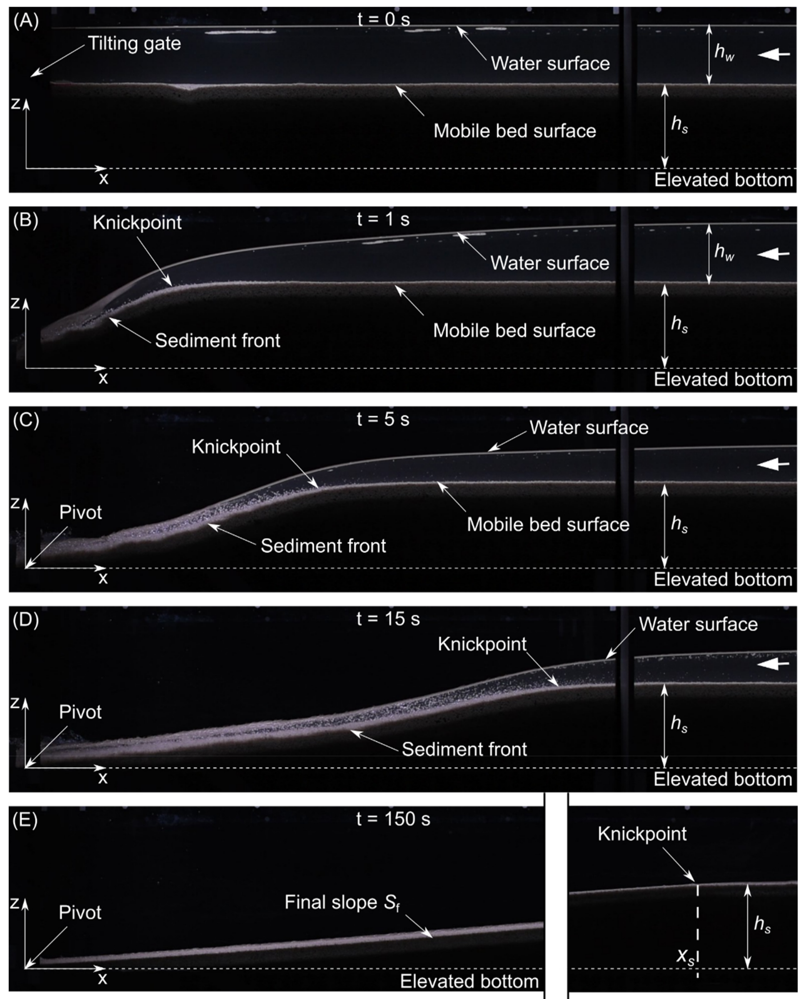
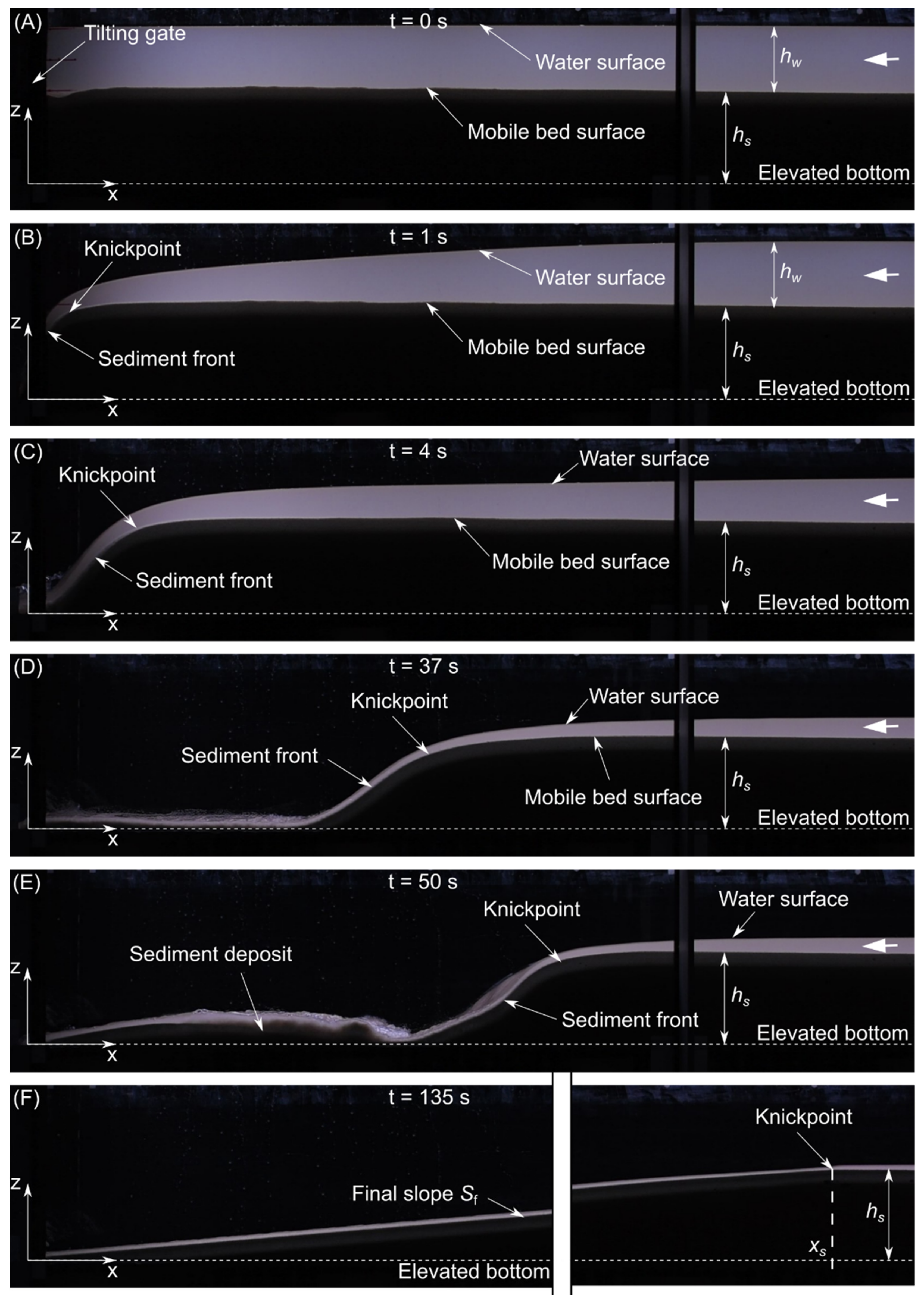
Every experiment began with a sudden opening of the tilting gate, which provoked a steep hydraulic gradient, flow acceleration, and rapid vertical erosion of the sediment front. This erosion led to the formation of a knickpoint that migrated upstream as the sediment front was eroded (Figure 3 and Figure 4). In this study, and according to [29], a knickpoint is that point at which the longitudinal slope of the bed changes abruptly (Figure 3 and Figure 4). The migration of the knickpoint was fast during the first instants of the experiments, and it was associated with intense sediment transport. For the coarse and medium sands, the sediment front pivoted around the edge of the elevated bottom at the downstream end, and its gradient decreased as the knickpoint migrated upstream (Figure 3). Meanwhile, the flow discharge gradually decreased until the initial volume of water (Vw) was completely evacuated. At the instant at which the flow was not enough to entrain any more sediments, the knickpoint ceased its migration and the sediment front reached the final slope (Sf) (Figure 3E and Figure 4F). In contrast, for the fine sand, the sediment front migrated upstream by keeping a roughly constant gradient, while downstream of the front, all sediments were transported by the flow (Figure 4D). This lasted until the transport capacity of the flow diminished and sediments began to deposit downstream of the sediment front. The deposited sediments and the sediment front merged gradually, creating a final bed surface with a uniform slope (Sf), similar to those observed for the coarse and medium sands (Figure 4E). Upstream of the knickpoint, no sediment transport was observed for any of the experiments. The aforementioned features are illustrated in Figure 3 and Figure 4, which depict the evolution of the bed and water surfaces of two representative experiments at different instants. These experiments were performed for hw L/hs2 = 26.65, Vw/hs3 = 54.73, S0 = 0.0% and for medium and fine sands (Figure 3 and Figure 4, respectively).
3.2. Sf for Varying Values of hw·L/hs2, D*, and S0
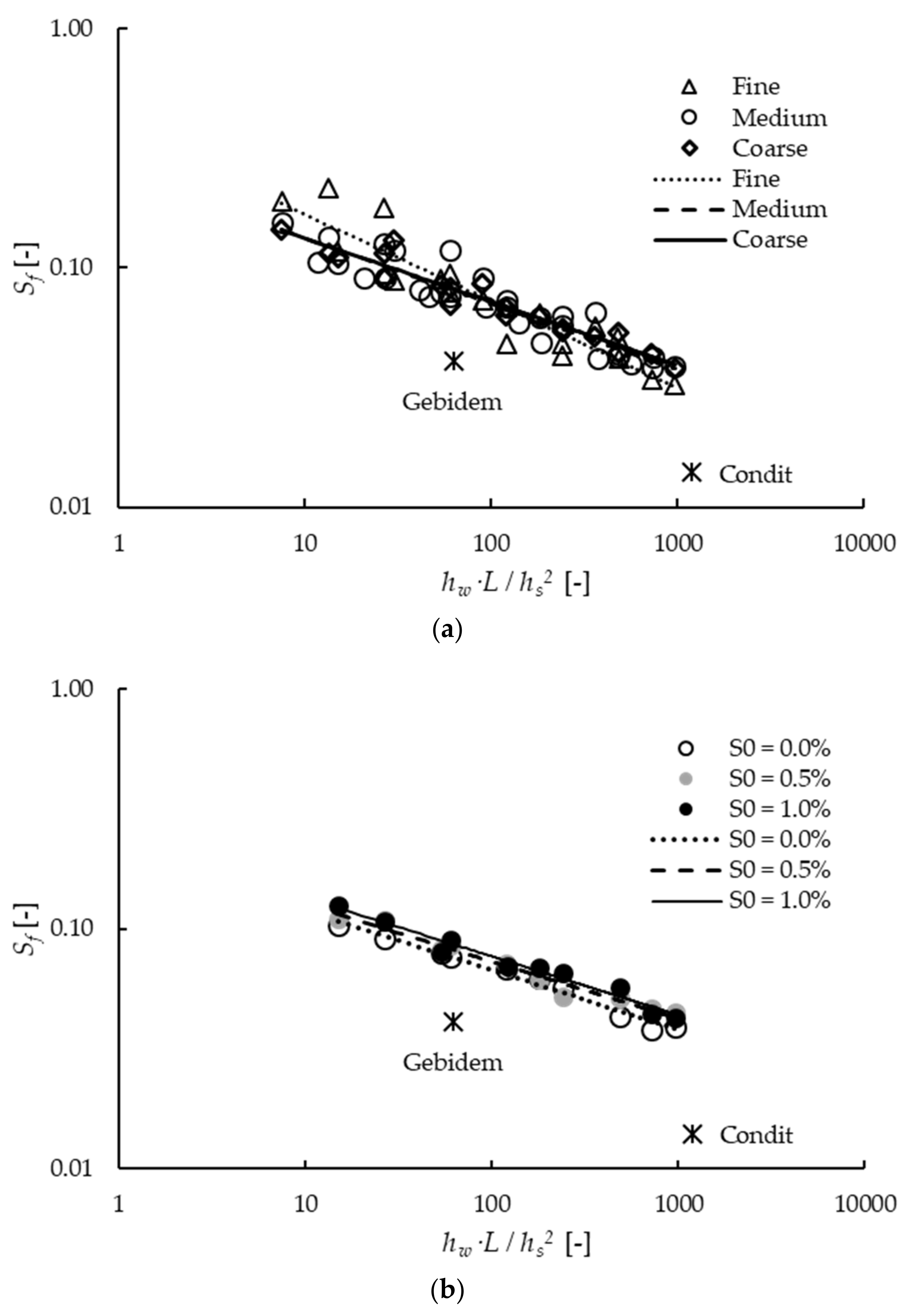
Figure 5a shows the evolution of Sf for the experiments performed for S0 = 0.0%, and for varying values of hw·L/hs2, and D*. In this experimental setup, the relative error ΔSf/Sf varies from 2% to 7%, with an average value of 4%, and Δ (hw·L/hs2)/hw·L/hs2 varies from 5% to 14%, with an average value of 9%. For the sake of clarity, error bars are not shown in the figure. Additionally, the values of Sf and hw·L/hs2 obtained for the flushing operations of the Gebidem and Condit dams are illustrated in Figure 5a. In this study, Sf was observed to decrease as the ratios hw/hs and L/hs increased individually (not shown). Hence, it is assumed that the evolution of Sf for varying values of hw·L/hs2 is also representative of the individual effects of hw/hs and L/hs on Sf. In these experiments, Sf decreased as the value of hw·L/hs2 increased. Namely, Sf ranged from 0.21 for hw·L/hs2 = 13 to 0.03 for hw·L/hs2 = 963. This trend was also observed when comparing the values obtained for the Gebidem and Condit dams, although the values of Sf obtained in this study were higher than those reported for the dams. In the present study, the values of Sf obtained for the coarse and medium sands were very similar, but they differed from those values obtained for the fine sand. Namely, for hw·L/hs2 < 134 approximately, the values of Sf obtained for the coarse and medium sands were lower than those obtained for the fine sand, whereas for hw L/hs2 > 134 and for the coarse and medium sands, Sf was steeper than for the fine sand. In some experiments, there were different values of Sf measured for the same value of hw·L/hs2. These were the cases in which, for a given value of hs, different values of hw and L led to the same value for the product hw·L. For instance, for hs = 0.05 m, those configurations in which hw = 0.05 m—L = 12.043 m and hw = 0.10 m—L = 5.997 m, both resulted in hw·L/hs2 = 240. In those cases, Sf increased as the ratio hw/L decreased, where hw/L denotes the initial hydraulic gradient of the reservoir. Regarding S0, the steeper it was, the steeper the Sf was. Nevertheless, it is important to note that, for given values of hw and L, Vw decreased as S0 increased. Hence, when comparing values of Sf measured for different values of S0, one must take into account that the initial volume of water (Vw) was also different. Therefore, the increase in Sf and the respective decrease in Vs must be attributed to the decrease in Vw, rather than to the increase in S0. Figure 5b shows the evolution of Sf for the experiments performed with medium sand, and for varying values of hw·L/hs2, and S0. In terms of the volume of sediment evacuated (Vs) and according to Equation (1), Vs increased as hw·L/hs2 and S0 increased. Regarding D*, for hw·L/hs2 < 134 the value of Vs was larger for the coarse and medium sands than for the fine sand, whereas for hw·L/hs2 > 134, the values of Vs obtained for the fine sand were larger than those obtained for the coarse and medium sands. Moreover, for a given value of hs and for a given value of hw·L, Vs was larger in those configurations with relatively low hydraulic gradients (hw/L).
3.3. Flushing Efficacy for Varying Values of Vw/hs3, S0 and D*
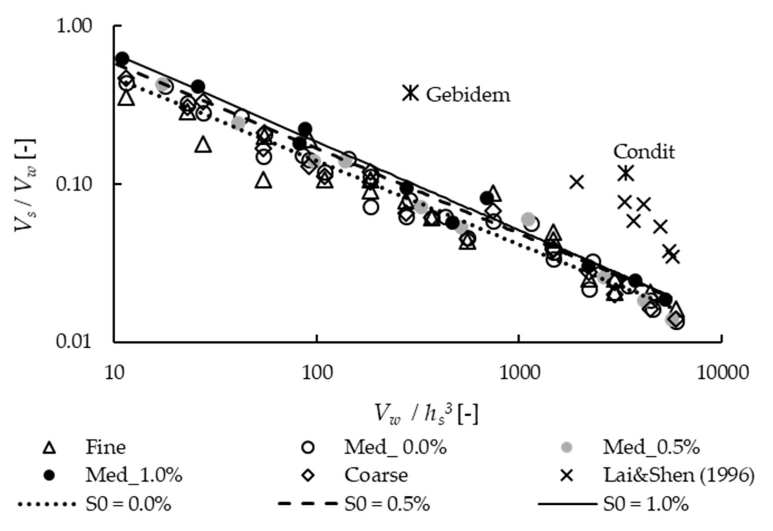
The evolution of the flushing efficacy (Vs/Vw) for varying values of Vw/hs3, S0 and D* is illustrated in Figure 6, along with the values of Vw/hs3 and Vs/Vw corresponding to the flushing operations of the Gebidem dam [2], the Condit dam [15], and those corresponding to the experiments performed by [24]. The results of this study show that Vs/Vw decreased as Vw/hs3 increased, for the three values of S0 and for the three values of D*. Namely, Vs/Vw varied from 0.63 for Vw/hs3 = 11 to 0.01 for Vw/hs3 = 79. The values of Vs/Vw obtained for the Gebidem and Condit dams, and for the experiments by [24], also decreased as Vw/hs3 increased. However, for a given value of Vw/hs3, the values of Vs/Vw measured in this study were lower than those obtained for the Gebidem and Condit dams and for the experiments by [24] (Figure 6). In this study, for the fine sand, the values of Vs/Vw measured for Vw/hs3 < 100 were lower than those measured for the coarse and medium sands. For those experiments with the same value of Vw/hs3 but different values for hw and L, the flushing efficacy increased as the ratio hw/L decreased (not shown). Regarding S0, the steeper it was, the higher the flushing efficacy (Vs/Vw) was. This pattern is highlighted in Figure 6 by means of three trend lines corresponding to each value of S0. These lines were obtained by means of Equation (13) (see below) for each value of S0. Equation (13) characterizes the influences of Vw/hs3, S0 and D* on Vs/Vw as:
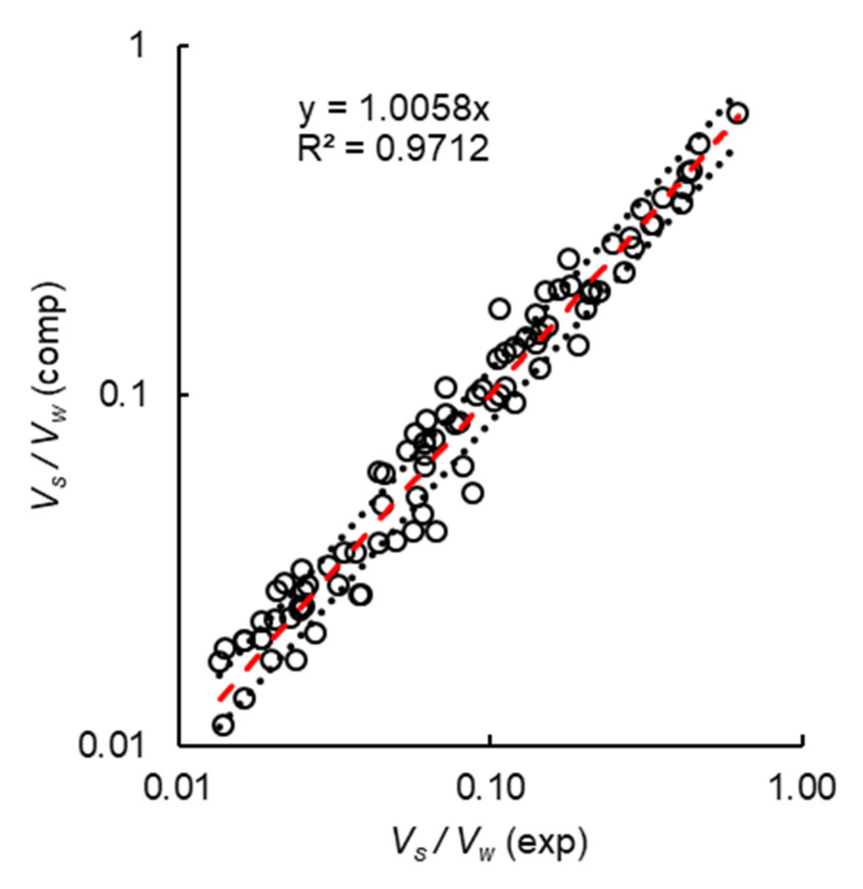
where the coefficients were calculated by means of the least square method, in order to obtain the best fitting curve for the whole dataset. Thus, Equation (13) provides the value of Vs/Vw as a function of Vw/hs3, S0 and D*; with an average relative error of ±17% regarding the values measured in the experiments. Figure 7 depicts the correlation between the values of Vs/Vw obtained from the experiments and those obtained by means of Equation (13), along with the error lines corresponding to ±17%.
4. Discussion
The experiments conducted in this study characterize the capacity of a stored volume of water to erode a mobile bed by means of flushing. The efficacy of the flushing (Vs/Vw) was evaluated for different initial conditions (hw, hs, Vw, S0) and for different sediment sizes (D*). During the experiments, the evolution of the bed morphology was characterized by: (i) an initial rapid and short vertical incision in the mobile bed that led to the formation of a knickpoint, (ii) a rapid upstream migration of it, accompanied by an intense sediment transport, retrogressive erosion, and bed degradation downstream of the knickpoint; and (iii) a slowdown of the knickpoint migration and a decrease in the sediment transport rate, downstream of the knickpoint. Finally, the bed profile was shaped by a roughly uniform slope (Sf) downstream of the knickpoint, and by an unaltered horizontal surface upstream of it (Figure 3E and Figure 4F). Similar patterns for the bed morphology are commonly observed in nature in those channels with a base-level lowering downstream, although the time scale of the process may vary significantly, depending on the case [15,16,28,29,30,31,32,33,34,35]. In nature, a base-level lowering leading to a knickpoint migration may originate either from natural processes [32], or from human interventions such as reservoir flushing or dam removals [2,15,16,35,36,37]. Typically, the upstream migration of the knickpoint is associated firstly with a rapid incision of the bed, and secondly with a slower widening of the incised channel. Initially, the incised channel may undergo narrowing, depending on the flow discharge [14]. In these experiments, bed erosion was uniform across the channel width, and hence, neither narrowing incision nor widening of it were observed. The absence of narrowing incision during the initial stage of the experiments can be attributed to the high flow discharge, resulting from both the sudden opening and the width of the outlet. The absence of channel widening can be attributed, on the one hand, to the full-width uniform erosion registered from the beginning of the experiments and, on the other hand, to the rigid lateral banks that impeded lateral erosion. The stages observed during the evolution of these experiments are analogous to those reported by [34], who characterized the channel response to dam removal by a conceptual model, including six stages. In this study, all the stages reported by [34] were registered, with the exception of stage D, which corresponds to channel widening. Stage B, in which the bed remains unaltered while the water level is lowering, was observed only upstream of the knickpoint, whereas downstream, stage C (degradation) followed stage A (pre-removal). Stage E, which characterizes bed aggradation downstream, was observed only for the experiments performed with fine sand (Figure 4E). Finally, the equilibrium of the bed (stage F) was reached when the flow discharge diminished and no more sediments were transported. Similar bed evolution, albeit with lateral erosion, was reported for the laboratory experiments by [14,24], and for the field observation during the removal of the Marmot and Condit dams in the USA [15,16], and after the failure of the Barlin dam in Japan [28].
The final bed slope registered downstream of the knickpoint (Sf) was observed to decrease as the value of hw·L/hs2 increased (Figure 5). Thus, the larger the initial volume of water per unit width (hw·L) was with respect to the thickness of sediments (hs), the lower Sf was and, consequently, the larger the volume of sediment evacuated (Vs) was. This pattern was also observed for the data reported for the flushing operations conducted at the Gebidem and Condit dams ([2] and [14], respectively) (Figure 5). Moreover, the lower values of Sf observed for those two dams with respect to the values obtained in this study are, presumably, owing to the lateral erosion. In these dams, the lateral erosion contributed to flattening the bed slope by bringing sediments into the incised channel.
In these experiments, Sf and, consequently, Vs were influenced by the sediment size, herein characterized by D*. The evolution of the experiments performed with fine sand and the results obtained from them differ from those obtained for the coarse and medium sands. These differences can be attributed to the existence of apparent cohesion in those mobile beds prepared with fine sand. These beds were not fully saturated owing to the unavoidable pores filled with air and confined within the soil matric. Apparent cohesion is typically observed in unsaturated granular soils, as a result of negative pressures exerted by capillary forces within the soil matric [38,39]. During the upstream migration of the knickpoint, this cohesion led to steep and roughly constant slopes of the sediment front [30]. This contrasts with the gradually decreasing and comparatively mild slope observed for the coarse and medium sands (Figure 3 and Figure 4). In addition, for the fine sand, the effect of the apparent cohesion was enhanced as hs increased and, consequently, hw·L/hs2 decreased. This resulted in comparatively high values of Sf for hw·L/hs2 < 134, with respect to the values of Sf measured for the coarse and medium sands. On the contrary, for relatively low values of hs (hw·L/hs2 > 134), the cohesion was weak and the values of Sf measured for the fine sand were lower than those measured for the coarse and medium sands.
In this study, and when comparing the data obtained for the Gebidem and Condit dams and for the laboratory experiments by [24], the efficacy of flushing, i.e., Vs/Vw, increases as Vw/hs3 decreases. This reveals that, although the volume of sediment evacuated from a reservoir increases as the volume of water increases, large increments in the volume of water only yield marginal increments in the volume of sediment evacuated. The higher values of efficacy registered for the Gebidem and Condit dams, and for the experiments by [24] with respect to the results of this study, can be attributed to lateral erosion. This erosion, not registered in this study, contributed by increasing in the total amount of sediments evacuated for a given volume of water, which resulted in higher values of Vs/Vw. In these experiments, the efficacy of flushing increases as the initial bed slope increases (S0), because steep bed slopes enhance the transport capacity of the flow. The effect of the sediment grain size (D*) on the efficacy of flushing was limited to that related to the apparent cohesion for the fine sand. Thus, in those experiments with high values of hs (low values of Vw/hs3), the efficacy of flushing measured for fine sand was lower than that measured for the coarse and the medium sands (Figure 6).
5. Conclusions
This study presents a comprehensive and systematic analysis of the effects of the initial volume of water, the initial water head, the bed slope, and the sediment grain size on the efficacy of flushing, when only the water previously stored in the reservoir is used. In addition, a group of dimensionless parameters have been derived to characterize this type of flushing. Nevertheless, the representativeness of the results obtained in this study is limited to those cases whose geometry, sediment characteristics, and initial conditions are within the range of values of the parameters tested in this study.
The results show that the volume of sediments evacuated from the reservoir increases as the initial volume of water and the bed slope increase. However, for relatively high initial volumes of water, only marginal increments in the volume of sediments evacuated were obtained. Thus, the efficacy of flushing, i.e., the ratio of the volume of sediments to the volume of water released, increases with the bed slope and decreases as the initial volume of water increases. These trends are corroborated by previous studies based on field observations and laboratory experiments. Nevertheless, owing to the absence of lateral erosion in these experiments, the values obtained in this study for the volume of sediments evacuated and for the efficacy of flushing are lower than those reported in previous studies, in which lateral erosion exists.
Regarding the sediment size, the results obtained for the fine sand differed from those obtained for the medium and coarse sands, owing to the existence of apparent cohesion in the sediment beds prepared with fine sand. The effect of this cohesion was significant in the experiment performed with relatively thick layers of fine sand, i.e., high values of hs; whereas for the experiments performed with relatively thin layers of fine sand, the effect of the apparent cohesion was negligible. Specifically, for a given volume of water, the apparent cohesion reduced the volume of sediment evacuated and hence, the efficacy of flushing, in comparison to those experiments performed with the medium and coarse sands. On the contrary, for those experiments performed with thin layers of fine sand, both the volume of sediment evacuated and the flushing efficacy were higher than those measured for the medium and coarse sands.
Author Contributions
All authors made a significant contribution to the research. S.G.-L. and J.A.T. performed the formal analysis of data and developed the methodology under the guidance and supervision of L.G.C. Results were thoroughly discussed by the three authors. All authors have read and agreed to the published version of the manuscript.
Funding
This study is part of the project EFISED (20403/SF/17) funded by the Fundación Séneca from Región de Murcia (Spain). The second author thanks the Escuela Politécnica Nacional (Ecuador), the Fundación Carolina (Spain), and Universidad Politécnica de Cartagena (Spain) for the financial aid received for his doctoral studies.
Institutional Review Board Statement
Not applicable.
Informed Consent Statement
Not applicable.
Data Availability Statement
The data presented in this study are available on request from the corresponding author. The data are not publicly available as they are part of broader ongoing research.
Conflicts of Interest
The authors declare no conflict of interest.
References
- Annandale, G.W.; Morris, G.L.; Karki, P. Extending the Life of Reservoirs: Sustainable Sediment Management for Dams and Run-of-River Hydropower; The World Bank: Washington, DC, USA, 2016. [Google Scholar] [CrossRef]
- Morris, G.L.; Fan, J. Reservoir Sedimentation Handbook: Design and Management of Dams, Reservoirs, and Watersheds for Sustainable Use, 1.04; McGraw-Hill Book Co.: New York, NY, USA, 1998. [Google Scholar]
- Kondolf, G.M.; Rubin, Z.K.; Minear, J.T. Dams on the Mekong: Cumulative sediment starvation. Water Resour. Res. 2014, 50, 5158–5169. [Google Scholar] [CrossRef]
- Franssen, N.R.; Tobler, M. Upstream effects of a reservoir on fish assemblages 45 years following impoundment. J. Fish Biol. 2013, 82, 1659–1670. [Google Scholar] [CrossRef] [PubMed]
- Bellmore, R.J.; Duda, J.J.; Craig, L.S.; Greene, S.L.; Torgersen, C.E.; Collins, M.J.; Vittum, K. Status and trends of dam removal research in the United States. Wiley Interdiscip. Rev. Water 2017, 4, e1164. [Google Scholar] [CrossRef]
- Schleiss, A.J.; Franca, M.J.; Juez, C.; De Cesare, G. Reservoir sedimentation. J. Hydraul. Res. 2016, 54, 595–614. [Google Scholar] [CrossRef]
- Mahmood, K. Reservoir Sedimentation: Impact, Extent, and Mitigation; Technical Paper WTP71; The World Bank: Washington, DC, USA, 1987. [Google Scholar]
- Sumi, T.; Okano, M.; Yasufumi, T. Reservoir sedimentation management with bypass tunnels in Japan. In Proceedings of the Ninth International Symposium on River Sedimentation, Yichang, China, 18–21 October 2004; pp. 1036–1043. [Google Scholar]
- Minear, J.T.; Kondolf, G.M. Estimating reservoir sedimentation rates at large spatial and temporal scales: A case study of California. Water Resour. Res. 2009, 45, 1–8. [Google Scholar] [CrossRef]
- Shrestha, B.; Babel, M.S.; Maskey, S.; van Griensven, A.; Uhlenbrook, S.; Green, A.; Akkharath, I. Impact of climate change on sediment yield in the Mekong River basin: A case study of the Nam Ou basin, Lao PDR. Hydrol. Earth Syst. Sci. 2013, 17, 1–20. [Google Scholar] [CrossRef]
- Guillén-Ludeña, S.; Manso, P.; Schleiss, A. Multidecadal Sediment Balance Modelling of a Cascade of Alpine Reservoirs and Perspectives Based on Climate Warming. Water 2018, 10, 1759. [Google Scholar] [CrossRef]
- Kondolf, G.M.; Gao, Y.; Annandale, G.W.; Morris, G.L.; Jiang, E.; Zhang, J.; Cao, Y.; Carling, P.; Fu, K.; Guo, Q.; et al. Sustainable sediment management in reservoirs and regulated rivers: Experiences from five continents. Earth’s Future 2014, 2, 256–280. [Google Scholar] [CrossRef]
- White, R. Evacuation of Sediments from Reservoirs; Thomas Telford Publishing: London, UK, 2001. [Google Scholar] [CrossRef]
- Cantelli, A.; Paola, C.; Parker, G. Experiments on upstream-migrating erosional narrowing and widening of an incisional channel caused by dam removal. Water Resour. Res. 2004, 40, 1–12. [Google Scholar] [CrossRef]
- Wilcox, A.C.; O’Connor, J.E.; Major, J.J. Rapid reservoir erosion, hyperconcentrated flow, and downstream deposition triggered by breaching of 38 m tall Condit Dam, White Salmon River, Washington. J. Geophys. Res. Earth Surf. 2014, 119, 1376–1394. [Google Scholar] [CrossRef]
- Major, J.J.; O’Connor, J.E.; Podolak, C.J.; Keith, M.K.; Grant, G.E.; Spicer, K.R.; Pittman, S.; Bragg, H.M.; Wallick, J.R.; Tanner, D.Q.; et al. Geomorphic Response of the Sandy River, Oregon, to Removal of Marmot Dam; U.S. Geological Survey: Reston, VA, USA, 2012. [CrossRef]
- Atkinson, E. The Feasibility of Flushing Sediment from Reservoirs; Report OD 137; HR Wallingford: Wallingford, UK, 1996. [Google Scholar]
- Batuca, D.G.; Jordaan, J.M. Silting and Desilting of Reservoirs; Taylor & Francis: Oxfordshire, UK, 2000. [Google Scholar]
- Di Silvio, G. Modeling Desiltation of Reservoirs by Bottom-Outlet Flushing. In Movable Bed Physical Models; Shen, H.W., Ed.; Springer: Dordrecht, The Netherlands, 1990; pp. 159–171. [Google Scholar] [CrossRef]
- Castillo, L.G.; Carrillo, J.M.; Álvarez, M.A. Complementary Methods for Determining the Sedimentation and Flushing in a Reservoir. J. Hydraul. Eng. 2015, 141, 05015004. [Google Scholar] [CrossRef]
- Dahal, S.; Crosato, A.; Omer, A.Y.A.; Lee, A.A. Validation of Model-Based Optimization of Reservoir Sediment Releases by Dam Removal. J. Water Resour. Plan. Manag. 2021, 147, 04021033. [Google Scholar] [CrossRef]
- Esmaeili, T.; Sumi, T.; Kantoush, S.; Kubota, Y.; Haun, S.; Rüther, N. Three-Dimensional Numerical Study of Free-Flow Sediment Flushing to Increase the Flushing Efficiency: A Case-Study Reservoir in Japan. Water 2017, 9, 900. [Google Scholar] [CrossRef]
- Esmaeili, T.; Sumi, T.; Kantoush, S.A.; Kubota, Y. Free-Flow Sediment Flushing: Insights from Prototype-Scale Studies. J. Disaster Res. 2018, 13, 677–690. [Google Scholar] [CrossRef]
- Lai, J.-S.; Shen, H.W. Flushing sediment through reservoirs. J. Hydraul. Res. 1996, 34, 237–255. [Google Scholar] [CrossRef]
- Shields, A. Application of similarity principles and turbulence research to bed-load movement. In Hydrodynamics Laboratory Publ. No. 167; Ott, W.P., van Uchelen, J.C., Eds.; U.S. Department of Agriculture, Soil Conservation Service Cooperative Laboratory, California Institute of Technology: Pasadena, CA, USA, 1936. [Google Scholar]
- van Rijn, L.C. Sediment Transport, Part I: Bed Load Transport. J. Hydraul. Eng. 1984, 110, 1431–1456. [Google Scholar] [CrossRef] [Green Version]
- Lai, J.-S. Hydraulic Flushing for Reservoir Desiltation; University of California, Berkeley: Berkeley, CA, USA, 1994. [Google Scholar]
- Tullos, D.; Wang, H.-W. Morphological responses and sediment processes following a typhoon-induced dam failure, Dahan River, Taiwan. Earth Surf. Process. Landf. 2014, 39, 245–258. [Google Scholar] [CrossRef]
- Begin, Z.B.; Schumm, S.A.; Meyer, D.F. Knickpoint Migration due to Baselevel Lowering. J. Waterw. Port Coast. Ocean Div. 1980, 106, 369–388. [Google Scholar] [CrossRef]
- Brush, L.M.J.; Wolman, M.G. Knicpoint behavior in noncohesive material: A laboratory study. GSA Bull. 1960, 71, 59–74. [Google Scholar] [CrossRef]
- Schumm, S.A.; Mosley, M.P.; Weaver, W.E. Incised Channels. In Experimental Fluvial Geomorphology; John Wiley & Sons, Ltd.: Hoboken, NJ, USA, 1987; pp. 192–225. [Google Scholar]
- Loget, N.; Van Den Driessche, J. Wave train model for knickpoint migration. Geomorphology 2009, 106, 376–382. [Google Scholar] [CrossRef]
- Shepherd, R.G.; Schumm, S.A. Experimental study of river incision: Discussion and reply. Geol. Soc. Am. Bull. 1976, 87, 320. [Google Scholar] [CrossRef]
- Doyle, M.W.; Stanley, E.H.; Harbor, J.M. Geomorphic analogies for assessing probable channel response to dam removal. J. Am. Water Resour. Assoc. 2002, 38, 1567–1579. [Google Scholar] [CrossRef]
- Pizzuto, J. Effects of dam removal on river form and process. Bioscience 2002, 52, 683–691. [Google Scholar] [CrossRef]
- Doyle, M.W.; Stanley, E.H.; Harbor, J.M. Channel adjustments following two dam removals in Wisconsin. Water Resour. Res. 2003, 39, 1–15. [Google Scholar] [CrossRef]
- MacBroom, J.G. Evolution of Channels Upstream of Dam Removal Sites. In Proceedings of the Managing Watersheds for Human and Natural Impacts, Williamsburg, VA, USA, 19–22 July 2005; pp. 1–12. [Google Scholar] [CrossRef]
- Bento, A.M.; Amaral, S.; Viseu, T.; Cardoso, R.; Ferreira, R.M.L. Direct Estimate of the Breach Hydrograph of an Overtopped Earth Dam. J. Hydraul. Eng. 2017, 143, 06017004. [Google Scholar] [CrossRef]
- Pickert, G.; Weitbrecht, V.; Bieberstein, A. Breaching of overtopped river embankments controlled by apparent cohesion. J. Hydraul. Res. 2011, 49, 143–156. [Google Scholar] [CrossRef]
Figure 1.
Sketch of the experimental facility. Not to scale.

Figure 2.
(a) Lateral view of the experimental facility just before the beginning of one experiment. (b) Lateral view of the experimental facility at the end of the experiment.
Figure 2.
(a) Lateral view of the experimental facility just before the beginning of one experiment. (b) Lateral view of the experimental facility at the end of the experiment.

Figure 3.
Lateral view of the experiment performed with medium sand, hw·L/hs2 = 26.65, Vw/hs3 = 54.73, and S0 = 0.0% at the instants: (A) t = 0 s, (B) t = 1 s, (C) t = 5 s, (D) t = 15 s, and (E) t = 150 s.
Figure 3.
Lateral view of the experiment performed with medium sand, hw·L/hs2 = 26.65, Vw/hs3 = 54.73, and S0 = 0.0% at the instants: (A) t = 0 s, (B) t = 1 s, (C) t = 5 s, (D) t = 15 s, and (E) t = 150 s.

Figure 4.
Longitudinal profiles of the bed surface and water surface for the experiment performed with fine sand, hw·L/hs2 = 26.65, Vw/hs3 = 54.73, and S0 = 0.0% at the instants: (A) t = 0 s, (B) t = 1 s, (C) t = 4 s, (D) t = 37 s, (E) t = 50 s, and (F) t = 135 s.
Figure 4.
Longitudinal profiles of the bed surface and water surface for the experiment performed with fine sand, hw·L/hs2 = 26.65, Vw/hs3 = 54.73, and S0 = 0.0% at the instants: (A) t = 0 s, (B) t = 1 s, (C) t = 4 s, (D) t = 37 s, (E) t = 50 s, and (F) t = 135 s.

Figure 5.
(a) Evolution of Sf for S0 = 0.0% and for varying values of hw·L/hs2 and D*. (b) Evolution of Sf for medium sand and for varying values of hw·L/hs2 and S0.
Figure 5.
(a) Evolution of Sf for S0 = 0.0% and for varying values of hw·L/hs2 and D*. (b) Evolution of Sf for medium sand and for varying values of hw·L/hs2 and S0.

Figure 6.
Evolution of Vs/Vw for varying values of Vw/hs3, S0, and D*.

Figure 7.
Correlation between the values of Vs/Vw obtained from the experiments and those computed with Equation (13). Dotted lines correspond to a relative error of ±17%.
Figure 7.
Correlation between the values of Vs/Vw obtained from the experiments and those computed with Equation (13). Dotted lines correspond to a relative error of ±17%.


Table 1.
Adopted values for the governing variables and parameters.
| hw·L/hs2 | Vw/hs3 | S0 | D* |
|---|---|---|---|
| [-] | [-] | [%] | [-] |
| Min = 7.5 Max = 963.4 | Min = 11.5 Max = 5934.8 | 0.0 0.5% 1.0% | 10 (Fine) 20 (Medium) 39 (Coarse) |
Table 2.
Values for the variables and parameters obtained from previous studies for comparison.
| Dam/Experiment | Data Source | L | hw | hs | Vw | Vs | Sf | hw·L/hs2 | Vw/hs3 | Vs/Vw |
|---|---|---|---|---|---|---|---|---|---|---|
| [m] | [m] | [m] | [m3] | [m3] | [-] | [-] | [-] | [%] | ||
| Condit (USA) | [15] | 2900 | 25 | 8 | 1.6 × 10⁶ | 1.8 × 10⁵ | 1.4% | 1192 | 3354 | 12% |
| Gebidem (CH) | [2] | 450 | 13 | 10 | 0.3 × 10⁶ | 1.0 × 10⁵ | 4.1% | 62 | 292 | 38% |
| Lai and Shen Run 1 | [27] | 33 | 0.07 | 0.1 | 5.53 | 0.21 | - | 230 | 5530 | 4% |
| Lai and Shen Run 2 | 22 | 0.07 | 0.1 | 3.69 | 0.22 | - | 154 | 3691 | 6% | |
| Lai and Shen Run 3 | 42 | 0.03 | 0.1 | 3.31 | 0.26 | - | 138 | 3313 | 8% | |
| Lai and Shen Run 4 | 24 | 0.07 | 0.1 | 4.13 | 0.31 | - | 172 | 4134 | 7% | |
| Lai and Shen Run 6 | 35 | 0.07 | 0.1 | 5.75 | 0.20 | - | 239 | 5747 | 3% | |
| Lai and Shen Run 7 | 30 | 0.07 | 0.1 | 4.98 | 0.27 | - | 208 | 4982 | 5% | |
| Lai and Shen Run 8 | 36 | 0.02 | 0.1 | 1.93 | 0.20 | - | 80 | 1930 | 10% |
Publisher’s Note: MDPI stays neutral with regard to jurisdictional claims in published maps and institutional affiliations. |
© 2022 by the authors. Licensee MDPI, Basel, Switzerland. This article is an open access article distributed under the terms and conditions of the Creative Commons Attribution (CC BY) license (https://creativecommons.org/licenses/by/4.0/).
Share and Cite
MDPI and ACS Style
Guillén-Ludeña, S.; Toapaxi, J.A.; Castillo, L.G. Flushing Capacity of a Stored Volume of Water: An Experimental Study. Water 2022, 14, 2607. https://doi.org/10.3390/w14172607
AMA Style
Guillén-Ludeña S, Toapaxi JA, Castillo LG. Flushing Capacity of a Stored Volume of Water: An Experimental Study. Water. 2022; 14(17):2607. https://doi.org/10.3390/w14172607
Chicago/Turabian StyleGuillén-Ludeña, Sebastián, Jorge A. Toapaxi, and Luis G. Castillo. 2022. "Flushing Capacity of a Stored Volume of Water: An Experimental Study" Water 14, no. 17: 2607. https://doi.org/10.3390/w14172607
Note that from the first issue of 2016, this journal uses article numbers instead of page numbers. See further details here.