Understanding the Effect of Hydro-Climatological Parameters on Dam Seepage Using Shapley Additive Explanation (SHAP): A Case Study of Earth-Fill Tarbela Dam, Pakistan

Abstract

For better stability, safety and water resource management in a dam, it is important to evaluate the amount of seepage from the dam body. This research is focused on machine learning approach to predict the amount of seepage from Pakistan’s Earth and rock fill Tarbela Dam during 2003 to 2015. The data of temperature, rainfall, water inflow, sediment inflow, reservoir level collected during 2003 to 2015 served as input while the seepage from dam during this period was the output. Artificial Neural Network (ANN), Random Forest (RF), Support Vector Machine (SVM), and CatBoost (CB), have been used to model the input-output relationship. The algorithms used to predict the dam seepage reported a high R² scores between actual and predicted values of average seepage, suggesting their reliability in predicting the seepage in the Tarbela Dam. Moreover, the CatBoost algorithm outperformed, by achieving an R² score of 0.978 in training, 0.805 in validation, and 0.773 in testing phase. Similarly, RMSE was 0.025 in training, 0.076 in validation, and 0.111 in testing phase. Furthermore, to understand the sensitivity of each parameter on the output (average seepage), Shapley Additive Explanations (SHAP), a model explanation algorithm, was used to understand the affect of each parameter on the output. A comparison of SHAP used for all the machine learning models is also presented. According to SHAP summary plots, reservoir level was reported as the most significant parameter, affecting the average seepage in Tarbela Dam. Moreover, a direct relationship was observed between reservoir level and average seepage. It was concluded that the machine learning models are reliable in predicting and understanding the dam seepage in the Tarbela Dam. These Machine Learning models address the limitations of humans in data collecting and analysis which is highly prone to errors, hence arriving at misleading information that can lead to dam failure.

1. Introduction

The Climate-Water-Energy-Food nexus is the hot topic of current scientific research directly linked to water resources [1]. The global fixed available water resource is becoming scarce due to human consumption, increasing population, industrialization, global warming, and climate change around the globe, especially in Asian countries [2,3]. 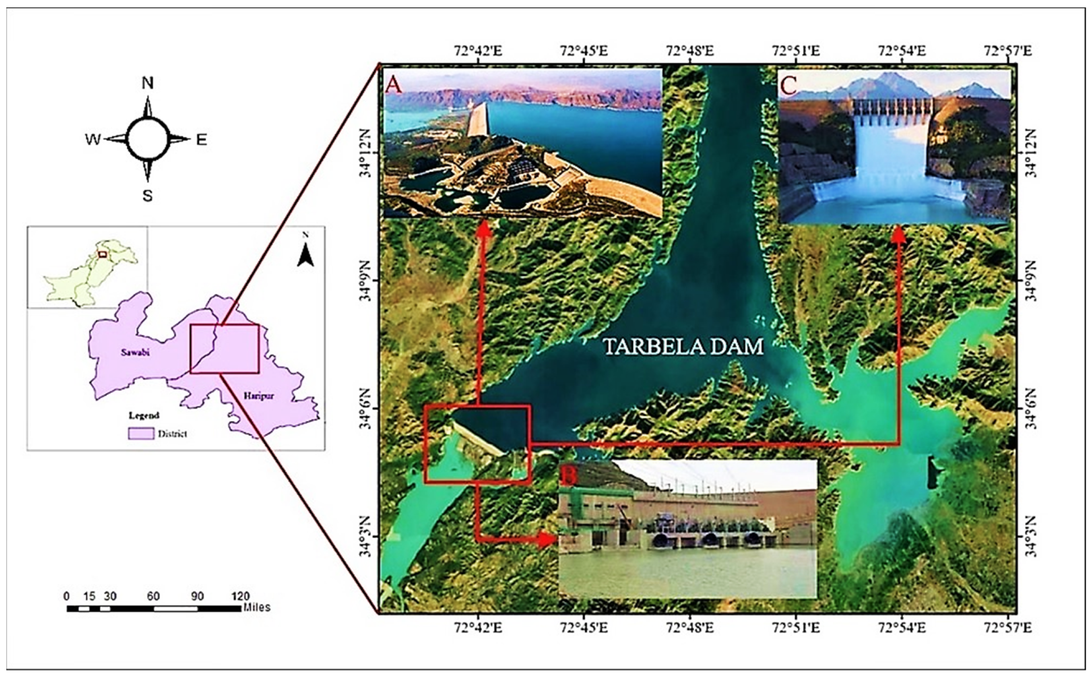Economic growth and environmental developments are being realized to develop new water storage projects (Dams and Canal systems) that yield sustainable water resource management [4]. Conservation of water resources is of utmost importance in recent times. Dams are the important infrastructure for power generation, agriculture and water resource management which has been under the influence of climatic deformation over the last decade. Earth fill dams such as the Tarbela Dam in Pakistan is the most important reservoir, which provides 52% of irrigation and 30% of hydropower generation needed for the country [5,6]. This reservoir plays an important role in melted glacier freshwater conservation flowing through the Indus river into the Tarbela Dam [7]. The seepage of water in dams is the a critical problem for any dam foundation. Seepage is defined as the slow movement of water from an upstream side to the downstream side from the body or foundation of dam. Controlling the seepage problem in a dam ensures the health stability of the dam. On the contrary, uncontrollable seepage is critical for dam stability and may cause water losses with dam structural failure. Seepage in dams is a consequence of the following reasons: The increase in water level from the desired limit [8,9], poor quality construction material used in Dams rehabilitation works [10], Earthquake and Artificial seismicity generated in Dams [11], Unconsolidated soil property [12], Joint and fracture in Dams structures [13].

The seepage inspection has been carried out using the geophysical base investigation to diagnose the seepage flow through the dam [14,15,16]. Several real-world concerns are connected to dam management, safety, and stability that can only be addressed by accurately calculating the seepage flow and its variability [17]. The statistics from previous literature show that dam failure due to seepage accounts for 30–40% of total dam failure [18]. The laboratory-based physical model experiment proves that the increase in seepage appreciably affects the health of dam [19]. This reason has led the dam management authority to continuously monitor the dam seepage throughout its life [20]. Dam safety can be evaluated by measuring the seepage flow in real-time daily monitoring. Such analysis is important during the construction phase of the dam structure. According to Adamo and Al-Ansari the precise detection of seepage flow can help to improve the anti-seepage with advanced scientific techniques, especially in peak sessions of water inflow in dam reservoirs [21,22]. In an earth-fill dam, seepage is important as it has been one of the major causes of dam failure in the past [23]. To avoid the dam failure problem, it is recommended to detect seepage flow for fast and accurate warning. Globally all countries agree that these dams must undergo a regular assessment and diagnostic for improvement of the life of dam.

The seepage can be greatly influenced by climatic parameters, water inflow, reservoir level, sedimentation load, and soil properties [24,25]. Water pressure is the main parameter used for seepage measurement with the help of a piezometer tube that has been largely adopted for tracking the seepage flow [26]. These parameters require extensive instrumental installation for the measurement of seepage flow [27]. Many earth-fill dams have proven the importance and applicability of geophysical methods in dam site investigations and safety monitoring. Dam seepage problems can be diagnosed using geophysical instruments on both the surface and the subsurface. For example, the Abu Baara earth dam in northeastern Syria was studied [28], where electrical resistivity tomography (ERT) survey was conducted, and the presence of cracked and karstified limestone rocks was discovered in ERT sections. Within the fragmented bedrock, several underlying structural anomalies were also discovered. [29] used Electrical resistivity tomography to identify subsidence anomalies in the body of an embankment dam in Iran, and the efficiency of this technique for the observed subsidence was confirmed. There are several geophysical techniques used for the dam seepage problem which are Electromagnetic profiling [30], Electrical resistivity Tomography [28], Self-potential methods [31], Ground penetrating radar [32], and Seismic methods [33]. These precise and reliable tools are used to check the health and monitor the dam stability and safety caused by a structural internal problem. Adamo et al. [21] discussed in detail the application of geophysical methods and their applicability in dam stability and safety monitoring.

Earth-fill dams are more prone to internal erosion and leaking due to seepage problems. Deterministic approaches for precisely estimating seepage flow through these dams have been studied in the literature [34]. Seepage analysis shows that if there is enough silty sand soil, the best design is a homogeneous earth-fill dam with a medium drain length and a thickness of 0.5 m. This seepage analysis depends on an equation describing water flow through a porous medium that follows Darcy law. Seepage volume, flow path, and velocity are all important considerations when assessing the structural behavior of a dam, all of which represent serious threats to the structure’s stability and security [35]. The finite element method has been used to measure as well as control seepage through embankment dams, among other techniques. [35,36,37,38,39,40,41,42,43,44,45,46,47,48,49], Finite difference method [50], weak form quadrature element method [51,52], and element free Method [53], etc. Recently [54] proposed a new approach to adjusting seepage issues through the earth-fill dam known as the multi-quadric method. Technological advancement has put seepage research in a new direction over the last decade, such as the integration of numerical modeling with machine learning, which can improve the seepage problem in the earth-fill dam and minimize the failure risk in water resources management system.

Many researchers have employed Machine Learning, and Artificial Intelligence (AI) based modeling to solve earth-fill dam seepage concerns in the last decade [55,56,57,58,59,60,61]. Previous research proves that AI methods are effective for dam seepage interpretation. For example, X. Zhang et al. [62] employed a genetic algorithm (GA) to optimize the weights and thresholds of a backpropagation neural network (BPNN), resulting in the development of the backpropagation neural network-Genetic Algorithm (BPNN-GA) seepage prediction model, which was used to increase dam seepage prediction accuracy and efficiency. Similarly, several different models are used in the literature for modeling water resources management problems, such as AI-based neural network [56,57,63,64,65], Genetic programming (GP) [66,67], Gaussian processes regression (GPR) [68], Support Vector Machine (SVM) [56,69], fuzzy logic and adaptive neuro-fuzzy inference system (ANFIS) [56]. Rehamnia, I. et. al. [57] investigated the estimation of dam seepage flow across concrete and embankment dams in Algeria using different algorithms (Support Vector Machine (SVM), M5Tree, and Multivariate Adaptive Regression Splines (MARS)) and discovered that SVM is more practical for doing so. The adaptive kernel extreme learning machine (KELM) approach developed by [69] was used to assess dam seepage. The researchers correlated the findings obtained using Multiple Linear Regression (MLR), Extreme Learning Machine (ELM), and Random Forest (RF). They discovered that the adaptive kernel extreme learning machine (EKLM) model performed well as compared to other models. Predicting seepage from observation data is an accurate strategy to assure dam stability. The rough set-Long short-term memory (RS-LSTM) model and Rough Set Theory have been used to predict the dam seepage pressure. As a result, it can do computations quickly and accurately [70].

Global warming and climatic changes trigger extreme metrological events such as rapid glacier melting, drought and heat waves worldwide and in Pakistan. These extreme events affect the normal trend of the hydrological cycle in terms of temperature, precipitation, sediment transportation and water inflow in river Indus which effect the Tarbela Dam structural stability and safety. Tarbela Dam was constructed in 1974, which wasn’t constructed according to the latest standards, that ensures resilience against such extreme global climatic events. Geoscientists say hydro-climatological parameters play an important role in seepage control and measurement in earth-fill dams. Numerous studies have been undertaken to model the relationship between various input factors, such as hydraulic parameters [71], piezometric data [72], etc., and dam seepage. However, the effect of hydro-climatological parameters on dam seepage has not been investigated. Furthermore, the Artificial Intelligence (AI) techniques used to model dam seepage based on different input parameters focus more on the accuracy of predictions made by the models; however, the explainability of the model predictions is not studied, which is necessary to explain the individual effect of each input on the output parameter and understand the dam seepage problem in detail.

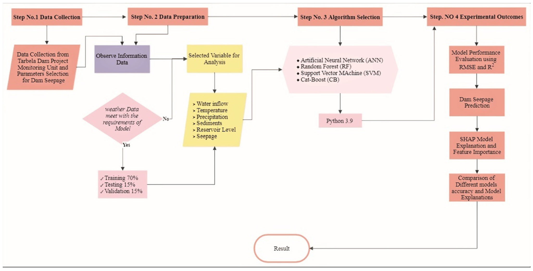
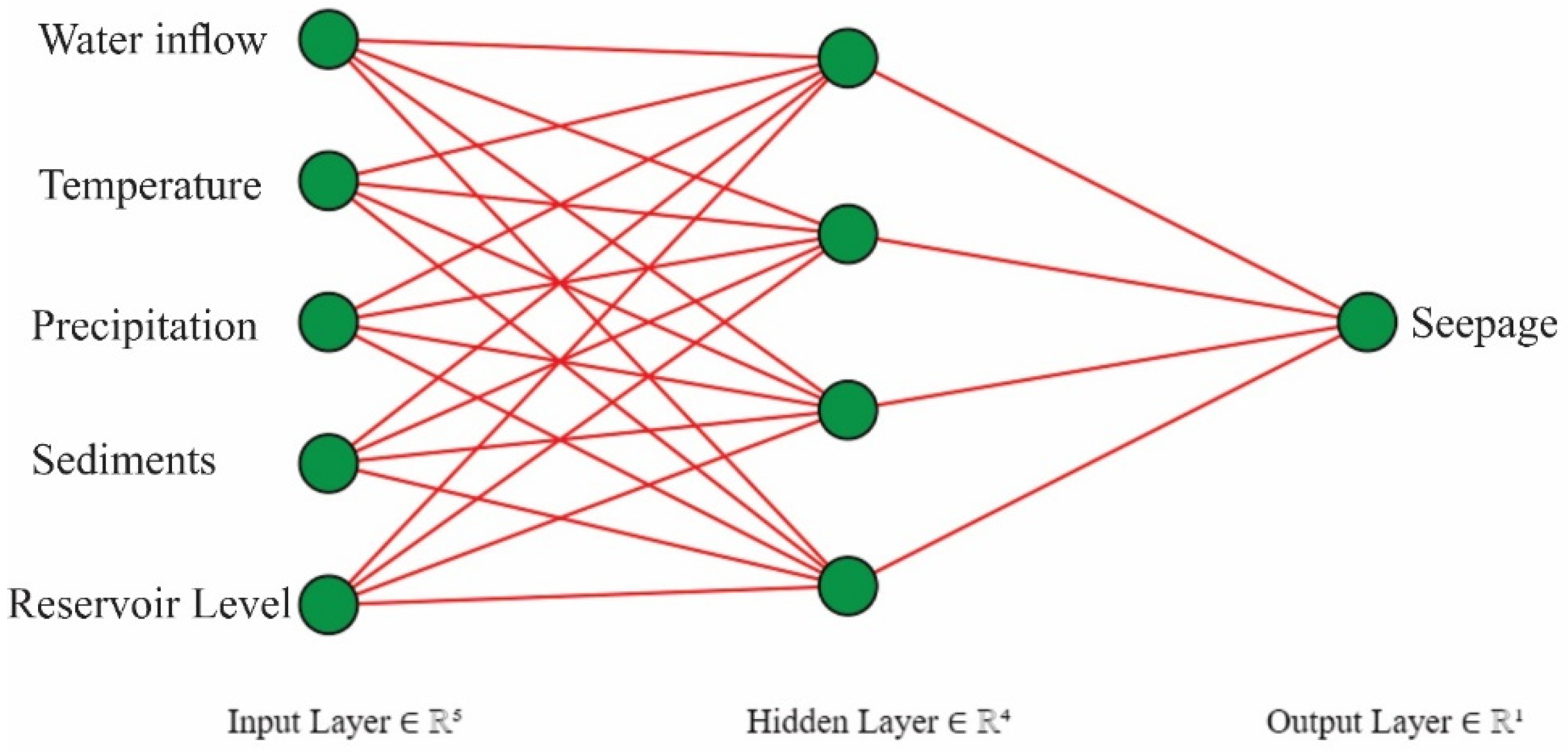
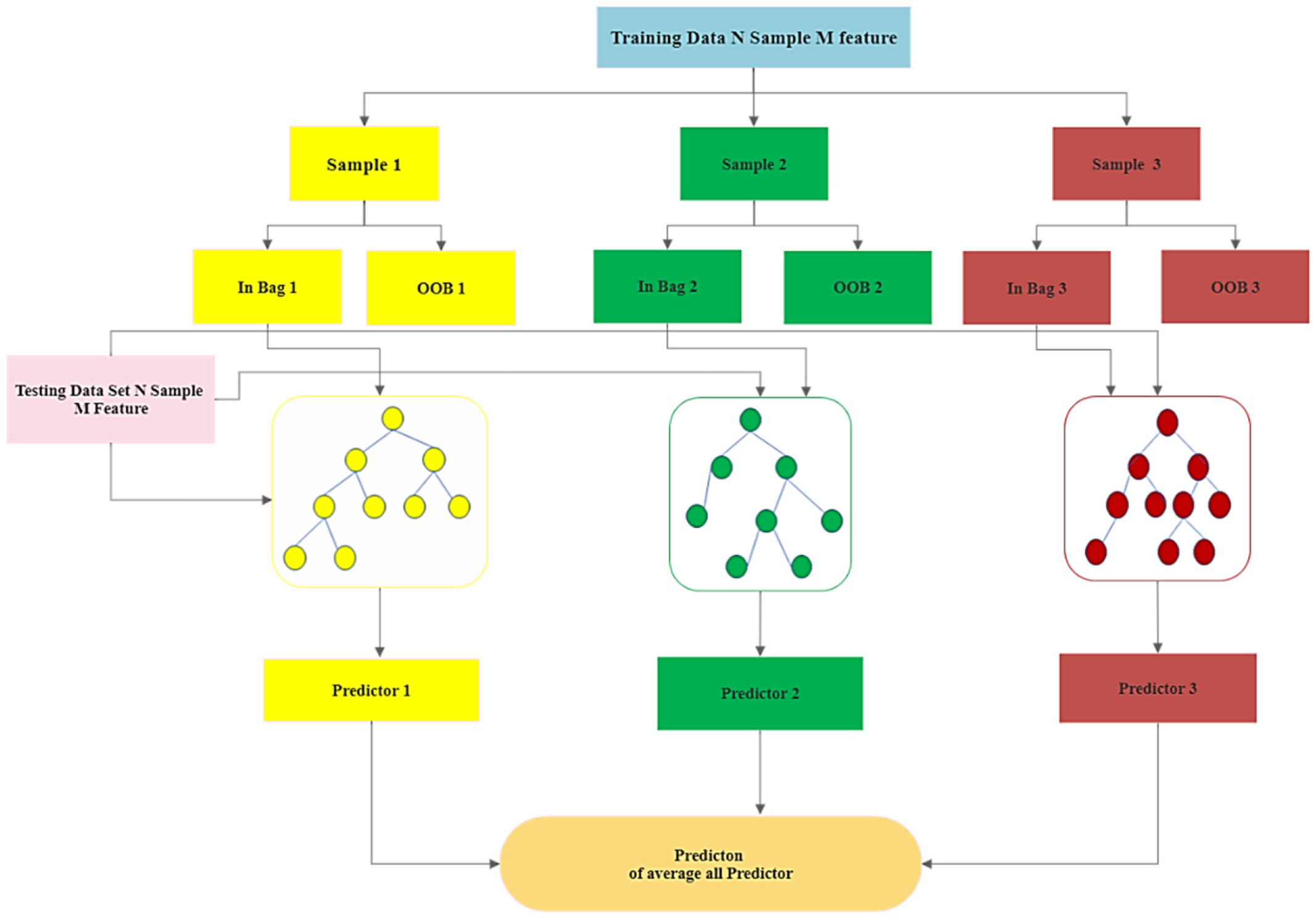
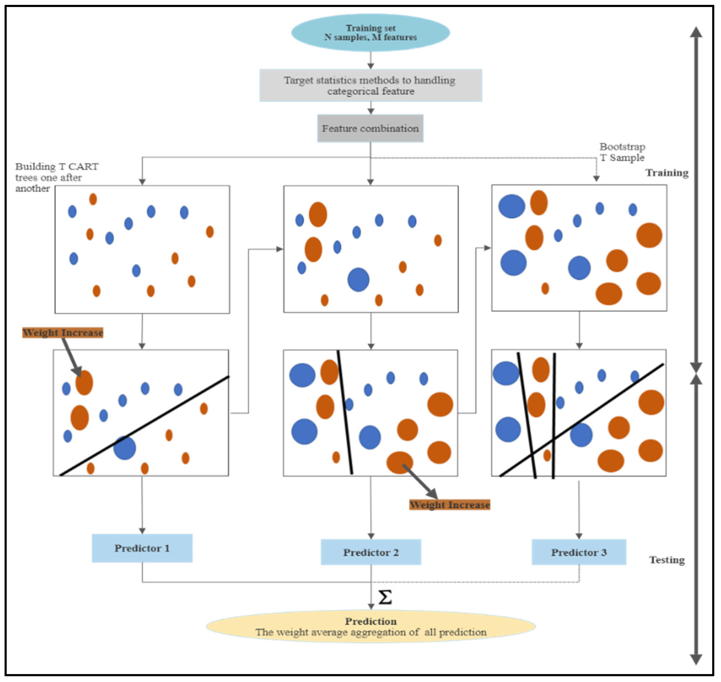
This study focuses on the use of different machine learning techniques to understand the effect of hydro-climatological parameters, i.e., temperature, precipitation, water inflow in the dam, sediment load, and reservoir level on the target, i.e., the average seepage in Tarbela Dam. Secondly, Shapley Additive Explanations (SHAP), a model explanation algorithm, was used to understand these Machine Learning (ML) algorithms’ model predictions, breaking down the predictions into individual feature impacts. Shapley Additive Explanations (SHAP) gives useful insight into the seepage problem in the Tarbela Dam and provides guidelines to control the seepage problem and avoid dam failure. The data collection was a difficult task because of the limited access to data on the dam site for research purposes. The data was gathered from Tarbela Dam project office and compiled for the experimental purposes. This study is organized into following (1) Modelling seepage based on hydro-climatological parameters using AI techniques, (2) Random forest (RF), CatBoost (CB), Artificial Neural Network (ANN) and Support Vector Machine (SVM) are used to predict Dam seepage, (3) Compare the Artificial Intelligence (AI) models accuracy in predicting dam seepage, (4) Use Explainable Artificial Intelligence (XAI) method, i.e., SHAP, to understand the model’s prediction and feature importance and (5) Emphasize the importance of Machine learning algorithms in resolving the dam seepage problem.

2. Materials and Methods

2.1. Study Area

Earth-fill Tarbela Dam is one of the world’s most massive dams situated in District Haripur, Khyber Pakhtunkhwa province of Pakistan [73]. The dam is 70 km in the northwest direction from Islamabad along the river Indus near Tarbela Village (Figure 1). The multipurpose earth-fill dam was initiated in 1970 and completed in 1974. It was built by Pakistan’s water and power development authorities to improve the low-cost hydropower energy, flood control, and water storage system for irrigation in Pakistan [74,75]. This dam is a significant public resource that supplies 50% of the country’s entire agriculture needs and 30% of its overall electric requirements [75]. The dam reservoir is over 100 km long and covers an area of 260 km square when filled. The live storage capacity of the dam reservoir was 11.9 billion m³, but this decreased to 6.8 billion m³ due to siltation throughout the reservoir’s 35-year operation. The Tarbela Dam is 2743 m in length and 143 m in height above the riverbed. It has two spillways, one of which cuts through the left bank and discharges into a ghazi broth pound at a downstream site, and the other cuts through the right bank. There are several important characteristics of the reservoir, including the catchment area (169,600 sq. km), measured annual water inflow in Tarbela Dam (64 Million-acer-feet (MAF)), the area of the lake (259 sq. km), live storage capacity designed for water (9.680 MAF), the present live storage (6.849 MAF), the maximum depth (137 m), the maximum elevation (472.44 m), the minimum operational elevation (420.01 m), the crest elevation (477 m), and the length of the crest (2743 m). The dam has two spillways, one of which is a service spillway with seven gates, and the other is an auxiliary spillway with nine gates. The installed capacity of the 4888-megawatt (MW) Tarbela Dam hydroelectric station will expand to 6298 MW following the completion of the 5th extension project, which is being financed by the Asian Infrastructure Development Bank and the World Bank.

2.2. Data Collection

The data was gathered from the Tarbela hydropower project monitoring unit, part of Pakistan’s water and power development authority (WAPDA). In this study, historically recorded information from 2003 to 2015 was selected for the experimental analysis. In the present study, selected variables (water inflow, reservoir level, temperature, precipitation, and sediment) of the potential data record of daily observed information were collected. The research flow chart is given below in Figure 2.

2.3. Algorithm Selection for Experiments

In this experiment, four machine-learning algorithms were used to model and predict the Earth-fill Tarbela Dam seepage. Machine learning algorithms learn and improve model performance using the training dataset. Generally, there are three types of Machines Learning, i.e., (i) supervised, (ii) unsupervised, (iii) reinforcement [76]. The conventional supervised regression framework was adopted for prediction of dam seepage. The parameter used in this study are presented in

Table 1. Input variable for Machine Learning Model.

S. No	Input Parameters	Unit	Duration	Output
1	Water Inflow	ft3/s	2003–2015	Average Seepage (m3/s)
2	Temperature	°C	2003–2015
3	Precipitation	Inches	2003–2015
4	Reservoir Level	Feet	2003–2015
5	Sediment Inflow	Tons	2003–2015

, and information about each model is given in

Table 2. The ML models description used for the experiments in python.

Algorithms	Python Module	Function	Symbols
Random Forest	sklearn. ensemble	Random Forest Regressor	RF
CatBoost	CatBoost. regression	Catboost Regressor	CB
Artificial Neural Network	keras. models. Sequential	Dense	ANN
Support Vector Machine	sklearn.SVC	SVR	SVR

.

2.3.1. Artificial Neural Network (ANN)

Artificial Neural Network (ANN) behavior is the same as a biological neural network and functions such as a human brain. ANNs can be trained to make predictions and learn about relationships without parameters using data sets [77,78]. These models find input-output relationships that don’t follow a straight line. However, ANN models only address the undefined mathematical relationship between the input and output data. The feed-forward neural network is the most common model of ANN, as shown in Figure 3. This model consists of three layers, i.e., (i). an input layer, (ii). hidden, and (iii). output layers. These layers consist of nodes fully connected to nodes in the other layers. The model has a feed-forward phase in which input signals move from one layer to the next until they reach the output layer and an error backward propagation phase that changes the strength of the connections (weights). An error is a discrepancy between target variable calculations and observations. Mathematically, the ANN model presented in the Equation (1) as below:

$$O_k=g_2\left[{\displaystyle \sum }_{j=1}^M{W}_{kj}{g}_1\left({\displaystyle \sum }_{i=1}^N{W}_{ji}{x}_i+W_{jo}\right)+W_{ko}\right]$$

(1)

From the above equation, notation is described as $x_i$ is that value goes into a node (i), $O_k$ value comes out from node k, $g_1$ is the activation function for the hidden layer (nonlinear) of the ANN model and similarly $g_2$ is the activation function for the output layer (linear). The input layer neuron numbers are N, and the hidden layer number of the neuron is M. The hidden neuron j and output neuron k have biases designated Wjo and Wko. Wji is the weight between i (input nodes) and j (hidden nodes), while Wkj is the weight between j (hidden nodes) and k (output nodes) nodes.

2.3.2. Random Forest

Breiman, L et al., [79] invented the random forest (RF) machine learning approach; It has been used in many different fields because it is very stable and can be used in many different situations [80]. RF is a collection of elementary decision trees, each formed by randomly selecting samples and attributes from all predictors, as shown in Figure 4 [81,82]. Most decision trees outputs are considered the RF’s final output [83]. Out-of-bag (OOB) samples are a subset of the samples that must be excluded from the original dataset. The mean square error (MSE) of OOB samples is often used to judge how well the RF method works (i.e., the sum of squared residuals from OOB samples should be divided by the sample size). It has been previously stated that the training and testing subsets (i.e., OOB samples) must be consistent to compare RF performance between different models. The number of trees in the forest (ntree) and the number of predictors tested at each node are important things to figure out during the RF model calibration process (mtry). The value of mtry was derived as per empirical methods provided in earlier research [83,84] to acquire the lowest possible generalization error and correlation between decision trees. RF model is mathematically written in Equation (2).

$$m_{try}=lo{g}_2\left(D+1\right)$$

$$m_{try}=\sqrt{D}$$

$$m_{try}=\frac{D}{3}$$

(2)

where D is the original dataset’s determined number of input variables, the N-tree is an important factor in forecasting; hence, an experiment was conducted to determine which n-tree to use. The RF model is trained, and model accuracy was evaluated with a rise in the number of trees until it reaches n_tree = 500.

2.3.3. Support Vector Machine

The Support Vector Machine (SVM) algorithm was introduced by Vapnik in 1995 [85]. It is a supervised learning strategy used for data analysis and pattern recognition. The SVM is known as a classifier or regression tool which analyzes two types of data, i.e., Linear and Nonlinear. The given N sample set ${\left\{L_k,M_k\right\}}_{k-1}^N.L\in R^m,M\in R$ here L is an input vector of m component and M is a corresponding output value, an SVM estimator $\left(f\right)$ on regression can be expressed.

$$f\left(L\right)=V\times \varnothing \left(L\right)+M$$

The weight vector is V, and the bias is M. Using the SVR, you can find the best V, and M. The input vectors are transferred into a high-dimensional feature space using the nonlinear transfer function u. A straightforward linear regression can theoretically handle the complex nonlinear regression of the input space. Usually, kernel function $k\left(x_i,x_j\right)=\left(\varnothing \left(x\_i \right).\varnothing \left(x\_j \right)\right)$ is used to acquire inner products in the feature space, and the computation can be carried out in the input space. In this study, the Gaussian radial basis function (RBF) with the form $k=\left(x_i,x_j\right)=exp\left(-\Vert x_i-x_j\Vert /2{\sigma }^2\right)$ was used. After acquiring the parameters ${\beta }_i,{\beta }_k^{*}$, and $B_{°}$, the final approximation function $f\left(L_i\right)$ is expressed in Equation (3).

$$f\left(L_i\right)={\displaystyle \sum }_{i=1}^n\left({\beta }_k-{\beta }_k^{*}\right)K\left(x_k,x_i\right)+B_{°}, K=1,\dots \dots \dots S$$

(3)

In this Equation (3), $x_k$ represents the support-vector, ${\beta }_k \mathrm{and} {\beta }_k^{*}$ are parameters connected through the support vector $x_k$ and n and s are the number of training samples and support vectors. To find the value of $f\left(L_i\right)$ that is ideal, it is necessary to optimize all three ($E, \epsilon , \sigma$) parameters.

2.3.4. CatBoost

CatBoost (CB) is an upgraded Gradient Boosting Decision Tree (GBDT) [86] toolkit comparable to Extreme Gradient Boosting (XGBoost) [87] that was introduced by Dorogush et al. in 2018 [88]. Gradient bias and prediction shifts are difficulties that CatBoost solves [89]. CatBoost is a unique ensemble-based learning method that performs regression, ranking, binary, and multiclass classification on categorical or numerical data [90]. CatBoost is a technique that is used for combining unbiased gradient boosting and deal categorical features (Figure 5). Its most essential characteristics remain its categorical properties and new order-boosting approach without forecasting shifts. It offers a variety of solutions that correspond to the various categories it covers. Instead of processing, its approach is optimized and implemented in the step where trees are divided, which is the preprocessing phase. Since only a few classes exist for each feature, the classifier uses one-hot encoding. This transforms the categorical features into numeric features with several associated occurrences. In the case of composite features, the classes and the average target are swapped. To prevent overfitting, the average sample $x_{\sigma i, k}$ is computed using the target values of the pictures that come before $x_{\sigma i, k}$ in an arbitrary permutation $\sigma =\left({\sigma }_1, {\sigma }_2,\dots \dots \dots {\sigma }_n\right)$ of the dataset defined by the Equation (4).

$$x_{\sigma i,k}=\frac{{{\displaystyle \sum }}_{j=1}^{i-1}\left[x_{\sigma i,k}=x_{\sigma j,k}\right] y_{\sigma j}+a\times p}{{{\displaystyle \sum }}_{j=1}^{i-1}\left[x_{\sigma i,k}=x_{\sigma j,k}\right]+a}$$

(4)

When the circumstance is fulfilled, $x_{\sigma i,k}=x_{\sigma i,k}$ Use value 1; p represents the prior value, and a represents the weights of the prior value. The regression task and prior probability are computed using the average of the entire dataset, P. This feature transformation will reveal the information loss of categorical character interaction. As a result, CatBoost (CB) considers the previous combination of features in their present condition and the remaining category qualities. CatBoost (CB) has a variable boosting arrangement based on a similar ordering concept and is useful for categorical traits to avoid overfitting. It works with trees that aren’t conscious of the splitting operations used throughout the tree’s construction. These trees take in information faster throughout the prediction stages, are proportionally stable, and do not exhibit overfitting. The ordered boosting mode was applied when CatBoost was employed. For each random permutation of the training data, n different trees are created as T1, …, Tn in the process of building an ordered boosting tree, to build the tree Ti using the first i examples in the permutations. The tree Tj−1 is used to determine the residual for the jth sample of the training data. The tree constructed using the training data at each permutation is used as a model for data prediction.

CatBoost (CB) begins building a tree by generating a p + 1 independent random permutation before switching to the boosting mode ordered for data training. To define the split evaluation in the internal nodes of the tree construction, the $\sigma =\left({\sigma }_1,{\sigma }_2,\dots \dots {\sigma }_n\right)$ permutations are put to use. In order to select the leaf values lj for the created tree, the σ₀ permutations are employed. Throughout the training, CatBoost (CB) maintains the supporting tree Tr,j where Tq,j (i) is the current prediction for the ith instance based on the initial j examples in the variation σ_r. In other words, Tq,j (i) is the current prediction for the ith instance. The information is then used to construct a tree. The operation of CatBoost (CB) is described in the Algorithm 1 as below.

Algorithm 1: CatBoost

Input:$\left\{\left({\mathit{X}}_{\mathit{k}}\mathbf{,}{\mathit{y}}_{\mathit{k}}\right)\right\}\mathbf{\forall } \mathit{K}\mathbf{=}\mathbf{1} \mathit{t}\mathit{o} \mathit{n}\mathbf{,} \mathit{I}$

$\mathbf{1}\mathbf{.} \mathit{\sigma }\mathbf{\leftarrow }\mathit{r}\mathit{a}\mathit{n}\mathit{d}\mathit{o}\mathit{a}\mathit{m} \mathit{P}\mathit{e}\mathit{r}\mathit{m}\mathit{u}\mathit{t}\mathit{a}\mathit{t}\mathit{i}\mathit{o}\mathit{n} \mathit{o}\mathit{f} \left[\mathbf{1}\mathbf{,}\mathit{n}\right]\mathbf{;}$

$\mathbf{2}\mathbf{.}\mathit{T}\mathit{i}\mathbf{\leftarrow }\mathbf{0} \mathit{f}\mathit{o}\mathit{r} \mathit{i}\mathbf{=}\mathbf{1}\mathbf{.}\mathit{n}\mathbf{;}$

$\mathbf{3}\mathbf{.}\mathit{f}\mathit{o}\mathit{r} \mathit{t}\mathbf{\leftarrow }\mathbf{1} \mathit{t}\mathit{o} \mathit{I} \mathit{d}\mathit{o}$

$\mathbf{4}\mathbf{.}\mathit{f}\mathit{o}\mathit{r} \mathit{i}\mathbf{\leftarrow }\mathbf{1} \mathit{t}\mathit{o} \mathit{n} \mathit{d}\mathit{o}$

$\mathbf{5}\mathbf{.}{\mathit{r}}_{\mathit{i}}\mathbf{\leftarrow }{\mathit{y}}_{\mathit{i}}\mathbf{-}{\mathit{T}}_{\mathit{\sigma }\left(\mathit{i}\right)\mathbf{-}\mathbf{1}}\left({\mathit{X}}_{\mathit{i}}\right)\mathbf{;}$

$\mathbf{6}\mathbf{.}\mathit{f}\mathit{o}\mathit{r} \mathit{i}\mathbf{\leftarrow }\mathbf{1} \mathit{t}\mathit{o} \mathit{n} \mathit{d}\mathit{o}$

$\mathbf{7}\mathbf{.}\mathsf{\Delta }\mathit{T}\mathbf{\leftarrow }\mathit{L}\mathit{e}\mathit{a}\mathit{r}\mathit{n}\mathit{T}\mathit{r}\mathit{e}\mathit{e}\left({\mathit{X}}_{\mathit{j}}\mathbf{,}{\mathit{r}}_{\mathit{j}}\right)\mathbf{:}\mathit{\sigma }\left(\mathit{j}\right)\mathbf{\le }\mathit{i}\mathbf{)}\mathbf{;}$

$\mathbf{8}\mathbf{.}{\mathit{T}}_{\mathit{i}}\mathbf{\leftarrow }{\mathit{T}}_{\mathit{i}}\mathbf{+}\mathsf{\Delta }\mathit{T}$

$\mathbf{9}\mathbf{.}\mathit{r}\mathit{e}\mathit{t}\mathit{u}\mathit{r}\mathit{n} {\mathit{T}}_{\mathit{n}}$

The CatBoost (CB) technique efficiently trains a boosting model based on random forest data. The Minimal Variance Sample (MVS) training system is a one-of-a-kind training approach introduced by the CatBoost (CB) algorithm. MVS is a regularization sampling technique that uses weighted sampling. The parameters needed to build each decision tree and those needed to set up the random forest model are both included in the CatBoost (CB) algorithm. Additionally, particular hyper-parameters must be built into the boosting process to train the model. While the boosting model is being trained, the CatBoost (CB) algorithm will take the hyper-parameters and optimize them. The settings are kept, and the trained model is accuracy-tested. The threshold parameters used in developing the random forest (RF) model can be specified using the saved parameters. CatBoost (CB) is an algorithm that enhances settings by saving hyper-parameters and using more data points.

2.4. Model Sensitivity

The interpretation of most machine learning models, such as evolutionary algorithms, deep neural networks etc., is difficult and is referred to as a “black box” [91,92]. Explainable Artificial Intelligence (XAI) algorithms have gained popularity in recent years, with XAI algorithms such as Shapley Additive Explanations (SHAP), Partial Dependence Plots (PDP), Accumulated Local Effects (ALE), and others being used to explain the predictions made by AI algorithms [93]. SHAP [91] is a novel technique for revealing the learned complexity of machine learning prediction models. It is an extremely useful tool for examining the relationship between individual variables and output variables because it decomposes predictions into individual feature impacts [94]. The SHAP feature relevance chart indicates the relative significance of each input variable affecting the output in absolute terms. The value assigned to an input feature’s relevance is determined by the mean absolute magnitude of the SHAP values across all instances. A summary plot of SHAP values illustrates how sensitive the output variable is to the input variable in question. The summary plot can depict the cause-and-effect relationship between the input characteristic’s high or low values (red to blue colors) and the corresponding SHAP value (of the output) on the horizontal axis.

A positive (SHAP value) on the horizontal axis indicates a direct association between high (red) and low (blue) values of the input variable. In comparison, input characteristics with a high (red) value reporting a negative (SHAP value) on the horizontal axis suggest an inverse link between the input and the output (response) variable, whereas a low (blue) value indicates a direct relationship between the input and the output. Jittered points densely packed on the chart represent the same SHAP value presented in various instances. SHAP dependence scatter plots illustrate the effect of a feature on the model’s predictions. The scatter plot represents a single prediction from the dataset. The x-axis indicates the feature’s value, while the vertical axis indicates the effect of the feature’s value on the model’s output. The color represents a secondary characteristic that combines with the primary characteristic.

SHAP [91] is a model-independent method that is based on game theory [95]. SHAP’s goal is to explain a prediction $f\left(x\right)$ of a specific instance $x$ by figuring out how much each feature value contributed to that specific outcome. The input to the explanation function g(.) is a coalition vector with the values $z\subset \left\{0,1\right\}N$, where N is the number of features in the original instance vector $x$. The coalition vector shows in a binary format whether each feature is present or not. An entry of 1 means that the corresponding feature adds to the explanation, while an entry of 0 means that the feature doesn’t add anything. It is understood that the explanation function $g\left(z^{\prime }\right)$ can be decomposed into these parts:

$$g\left(z^{\prime }\right)={\varphi }_0+{\displaystyle \sum }_{i=1}^N{\varphi }_i{z^{\prime }}_i,{\varphi }_i\in ℝ$$

Were as:

N = Number of input feature in x vector, the instant vector

$g=$ Explain the model

$z^{\prime }=$ contain vector such that $z\subset {\left\{0,1\right\}}^N$

${\varphi }_i=$ Decomposition factor

2.5. Data Preparation

The data was summarized from daily recorded information from 2003 to 2015 into a monthly average, i.e., one reading for each month. A total of 13 years of data was converted into the monthly format, and 156 samples were produced and analyzed in these experiments. After data processing, 156 observed information records were prepared yearly, including the water inflow, temperature, precipitation, reservoir level, and sediment load, and the average seepage of the Tarbela earth-fill dam in Table 1. The data is normalized between a value of 0–1 using the Mix-Max scaling function in python before feeding it to the machine learning model. No null values or outliers are reported. The dataset is divided into three subsets, i.e., training (70%), testing (15%) and validation (15%). The training dataset is used to train the machine learning models. The hyperparameters are tuned to acquire good results on both the training and validation subsets, whereas the testing dataset is used to check the performance and robustness of these models.

2.6. Descriptive Statistic

Descriptive statistics for all variables are presented in

Table 3. Descriptive statistic of parameters used for dam seepage prediction.

	Water Inflow	Reservoir Level	Temperature	Sediment Inflow	Precipitation	Average Seepage
	(ft3/s)	(ft)	(°C)	(Tn)	(In)	(m3/s)
	Training Data
Count	109	109	109	109	109	109
Mean	72.17	1449.13	18.34	9,363,574.31	82.64	8.17
Std	74.68	51.83	7.18	19,964,062.22	76.41	3.63
Min	13.21	1368.22	7.2	23,250.51	2.6	2.49
Max	277.08	1549.79	29.6	137,865,137.40	391	23.11
	Validation Data
Count	24	24	24	24	24	24
Mean	115.57	1494.62	21.96	23,653,407.21	119.14	10.18
Std	93.30	50.78	6.33	44,614,740.11	120.67	3.66
Min	16.57	1386.45	8.1	63,171.09	20.4	3.35
Max	357.51	1549.92	28.2	167,516,137.8	491.6	17.33
	Testing Data
Count	23	23	23	23	23	23
Mean	94.03	1466.60	22.29	9,694,283.85	86.06	9.28
Std	82.97	63.05	5.49	14,439,229.52	63.65	4.94
Min	16.72	1365.32	9.7	43,243.74	1.3	3.04
Max	296.30	1547.92	29	48,530,269.8	268.9	21.95

. The input and output variables’ minimums (Min), maximums (Max) is the maximum value of dataset, means, and standard deviations (std) are displayed. A standard deviation (SD) is a statistic that measures the range of values in a data set.

2.7. Model Evaluation Metrics

Model performance of machine learning (ML) models is evaluated using root-mean-squared (RMSE) coefficient of determination (R²) and Nash-Sutcliffe Efficiency (NSE). Many studies have shown the use of these metrics to measure accuracy in machine learning models [96,97]. R² value ranges from 0–1 but commonly written as 0–100%. Higher values R² closer to 1 indicate better fit whereas values less than 0.5 closer to zero indicate poor fit Similarly, RMSE value ranges from 0–∞, they are negative scores, means that lower values are preferable and indicate better performance of the model. NSE value range from 0–1 which is comparable with R². When NSE = 1.0, then it shows a perfect fit. NSE > 0.75 is a very good fit, NSE = 0.64–0.74 is a good fit. NSE = 0.5–0.64 is a satisfactory fit, and NSE < 0.5 is an unsatisfactory fit. RMSE R² and NSE were calculated using Equations no (5)–(7) to evaluate model accuracy.

$$RMSE=\sqrt{\sum \frac{{(A_t-B_t)}^2}{n}}$$

(5)

$$R^2=\frac{{\left[\sum \left(A_t-\overline{A_t}\right)\left(B_t-\overline{B_t}\right)\right]}^2}{\sum {\left(A_t-\overline{A_t}\right)}^2{\left(B_t-\overline{B_t}\right)}^2}$$

(6)

$$NSE=1-\frac{\sum {\left(A_t-B_t\right)}^2}{\sum {\left(A_t-\overline{B_t}\right)}^2}$$

(7)

Were $A_t$ is the actual value of t, $A_t$ is the mean of the actual value, $B_t$ is the estimated value of t, $B_t$ represent the estimated value mean, and the total number of times is denoted as n. Residual mean square errors (RMSE) measure the uncertainty in estimating the absolute error rates. When verification values are close to zero, observed and model values will be more similar. R² compares the probability of the predicted and actual values.

3. Results and Discussion

3.1. Correlation Matrix (Heat Map)

The correlation between different variables used in the data is presented in Figure 6, given below.

The heatmap of the correlation matrix shows the highest correlation coefficient of 0.77 between the Reservoir Level and the Average Seepage, followed by water inflow, Sediment Inflow, Precipitation, and Temperature. Figure 6 shows the water inflow and sediment inflow has a moderate correlation with average seepage, and temperature shows a low correlation with average seepage. From the correlation matrix, it is analyzed that sediment inflow also has the highest correlation with water inflow i.e., 0.81 which is due to downstream flow of river Indus that increases the sediment flowrate toward Tarbela Reservoir. Similarly, temperature and precipitation have a moderate to low correlation with water inflow. The Reservoir level has a significantly higher correlation than other hydro-climatological parameters used to predict the Average Seepage, indicating the importance of reservoir level in predicting seepage in dams.

3.2. Model Accuracy

Table 4. Prediction accuracy result of different Machine Learning Models.

Model	R2 Training	R2 Validation	R2 Testing	RMSE Training	RMSE Validation	RMSE Testing
	(m3/h)	(m3/h)	(m3/h)	(m3/h)	(m3/h)	(m3/h)
Random Forest Regression	0.884	0.801	0.782	0.059	0.077	0.109
Catboost Regression	0.978	0.805	0.773	0.025	0.076	0.111
Artificial Neural Network	0.981	0.835	0.715	0.245	0.249	0.297
Support Vector Regression	0.591	0.794	0.783	0.111	0.078	0.108

shows the model performance during training, validation and testing, i.e., root means square errors (RMSE) and coefficient of determination (R²) scores for the different models applied to predict the seepage of the Tarbela Dam. Catboost Regression model reports the best coefficient of determination (R²) scores of 0.978, 0.805, and 0.773 with the RMSE of 0.025, 0.076 and 0.111 on training, validation and testing datasets, respectively.

Table 5. Prediction accuracy result of Nash-Sutcliffe Efficiency for different Machine learning Models.

Nash-Sutcliffe Efficiency	Random Forest	CatBoost	SVR	ANN
Training	0.884	0.884	0.592	−212.980
Validation	0.803	0.806	0.799	−48.289
Testing	0.783	0.775	0.784	−34.416

shows the Nash-Sutcliffe Efficiency scores during training, validation and testing phase. CatBoost outperforms the algorithms with NSE scores 0.844, 0.806 and 0.775 during training validation, and testing phase, respectively. The worst performance was reported by ANN.

Figure 7 shows actual vs. predicted results during training, validation, and testing phases of the Random Forest (RF) (a), CatBoost (CB) (b), Artificial Neural Network (ANN) (c), and Support Vector Machine (SVM) (d) of Tarbela Dam seepage. Figure 7 on the x-axis shows the yearly observation, and the y-axis shows the average seepage.

The actual data shows seepage trend from 2003–2015; it is observed that, from 2003–2008 seepage trend was normal, but in 2008–2009 sudden increase is observed in the seepage, which was a consequence of increase in water inflow, sediment inflow and reservoir level due to extreme weather events in the region. Similarly, a decrease is seen in the seepage in 2010–2011, which was due heavy rainfall and flood in Tarbela Dam Pakistan in 2010; to reduce the influence of flood and heavy rainfall, water outflow was increased from the normal level for the health and safety purpose of the Tarbela Dam. Furthermore, it was also observed that from 2011–2014 seepage trend was slightly increasing due to the rise in temperature, precipitation effect.

Figure 8 displays the regression plots (RF, Catboost, ANN, and SVM), i.e., the actual vs. predicted values of average seepage for all the four models. The RMSE score shown in Table 3 is the least for the Catboost model, which is observed in Figure 8b where the points are clustered close to the regression line at low seepage values having a low error. However, at a high value of seepage, only a few points are far from the regression line having high error compared to other models, e.g., in the ANN model regression plot given in Figure 8c, one can observe most of the points lie very close to the regression line having a low error; however, some values lie very far apart from the regression line both at low and high values of seepage hence effecting the RMSE values highly. Similarly, Figure 8a shows the actual vs. predicted values for the random forest algorithm, which has an almost similar performance to the Catboost model. However, at the training phase, the samples are more spread around the regression plot than in the Catboost model; hence, the training RMSE for training given in Table 3 compared to the RMSE of the Random Forest Algorithm. Figure 8d shows the actual vs. predicted for the SVR model. The Figure 9 show the water inflow vs out flow comparision for 2003-2015 for reservoir level and seepage monitoring discussion with hydro-climatological variable. Similarly Figure 10 displays the regression plot for water inflow vs water out flow has a close correlation with each other which have a direct impact on reservoir level and effect dam seepage.

Machine Learning models are black-box models that do not explain the cause-and-effect relationship of parameters. However, SHAP gave some interesting insight into the cause-and-effect relationship between input (water inflow, Temperature, precipitation, sediment inflow and reservoir level) and output (seepage). The magnitude of feature importance is visualized in the SHAP feature importance charts given in Figure 11a–d. It is evident that the Reservoir Level is the most important feature in predicting the average seepage, as shown in Figure 12a–d.

3.3. Feature Importance

The effect of each input parameter on the output is visualized in the SHAP summary plot given in Figure 11a–d. The absolute magnitude of the effect of each feature is displayed in Figure 12a–d for all the models used to predict average seepage in the Tarbela Dam. The response of each feature to the output is explained separately in the paragraphs given below.

3.3.1. Reservoir Level

From Figure 11a–d, one can conclude a similar understanding, i.e., the reservoir level has a direct relationship with the seepage indicated by higher values of reservoir level (red dots) having positive SHAP values, suggesting, as the reservoir level increases the average seepage increases and vice versa. Furthermore, the magnitude of the effect of reservoir level on the average seepage is maximum compared to other features, shown in Figure 12a–d and the SHAP summary plot. As the reservoir level increases, the force of the water body exerted on the dam structure rises. The increasing pressure increases the water velocity in the seepage galleries; consequently, increasing the average seepage in the dam. Additionally, the reservoir level is also directly influenced by global warming and climate change. During the last decade, global warming and climate changes have impacted the Pakistan Tarbela Dam [98]. The Tarbela Dam’s source is the Indus River, which originated from the Mansarovar lake on the Tibetan plateau, and entered Pakistan from Ladakh, Baltistan and Gilgit [99]. For the last decade, Pakistan glaciers have been melting rapidly due to global warming and climate changes [100]. Tributaries from the glacier (Biafo, Baltoro, Batura) feed the Indus River system, increasing the inflow of water in the river Indus and influencing the reservoir level, especially in summer.

3.3.2. Temperature

Figure 11a–d shows that temperature has an inverse relationship with the seepage, i.e., lower Temperature values (red dots) have negative SHAP values, indicating lower temperature increases the average seepage and vice versa. The inverse relationship of temperature with average seepage can be explained as the consequence of the following effects:

During the summer season in Pakistan, the water outflow from the Tarbela Dam is increased due to irrigation demands; the reservoir level drops significantly, indirectly decreasing the average seepage; hence this effect is observed.

Similarly, the increasing temperature results in the increase in the evaporation of water from the dam, which also decreases the reservoir level, hence decreasing the average seepage in the Tarbela Dam.

Moreover, the magnitude of temperature on average seepage is visualized in Figure 12a–d for all the models used. According to RF, CatBoost and SVR Figure 12a,b,d, the temperature is the second most important parameter affecting average seepage; however, the magnitude of its effect is minimal compared to reservoir level except in ANN. According to Figure 12c, i.e., the ANN model, the effect of temperature on average seepage is the same as in Figure 12a,b,d, but the magnitude of its effect is almost similar to that of reservoir level and is the third most important parameter in influencing average seepage after reservoir level and sediment (Inflow).

3.3.3. Precipitation

Figure 11a–d shows that precipitation has an inverse relationship with the seepage, i.e., lower precipitation values (red dots) have negative SHAP values, indicating lower precipitation values increase the average seepage and vice versa. However, the magnitude of precipitation on the average seepage is negligible, as indicated by all the models in Figure 11a–d and Figure 12a–d.

3.3.4. Water Inflow

The magnitude of the effect of water inflow on Tarbela Dam seepage is minimal compared to other input features, as shown in Figure 12a–d. It is a common understanding that the dam’s water inflow increases. It causes a rise in the dam reservoir level, which in turn increases the stresses on the body of the dam, resulting in an increase in seepage in the seepage galleries. However, the SHAP summary plots shows no effect of water inflow on the seepage; this effect can be explained by observing water outflow along with inflow. Figure 10 compares water inflow and outflow from 2003 to 2015 in the Tarbela Dam. As the water inflow increases, the outflow is also increased to reduce the excess water coming into the dam. The same effect is visible in the Figure 12 regression plot, which is drawn between water inflow and outflow where all points lie close to the regression line, indicating the high correlation between both parameters and showing no effect on Tarbela Dam seepage for the year 2003 to 2015.

3.3.5. Sediment Inflow

From Figure 11a–d, one can conclude a similar understanding, i.e., the sediment has a direct relationship with the seepage, i.e., higher values of sediment (red dots) have positive SHAP values, which means as the sediment increase the average seepage increases and vice versa. The magnitude of sediment inflow on the average seepage is different according to all the models. Figure 12a,b Random Forests and Catboost model suggests the sediment have the second least and least magnitude of effect on average seepage, respectively. However, Figure 12c,d ANN and SVR show sediment as the second and third most important parameters influencing the average seepage. Similarly, the Figure 11c,d summary plots show a clear, direct effect on average seepage compared to Figure 11a,b summary plots. As sediment increase, the stresses on the foundation or body of the dam increase, causing a rise in the average seepage in the galleries.

These findings after model explanation are highly important for the industry in critical decision making, as it can help in taking control measures to prevent probable accidents by controlling certain parameters. Similarly, these findings are transferable to other similar dams and locations and may help in decision making, however, studying and modelling other site-specific data is recommended more due data variation, site conditions and many other parameters.

4. Conclusions

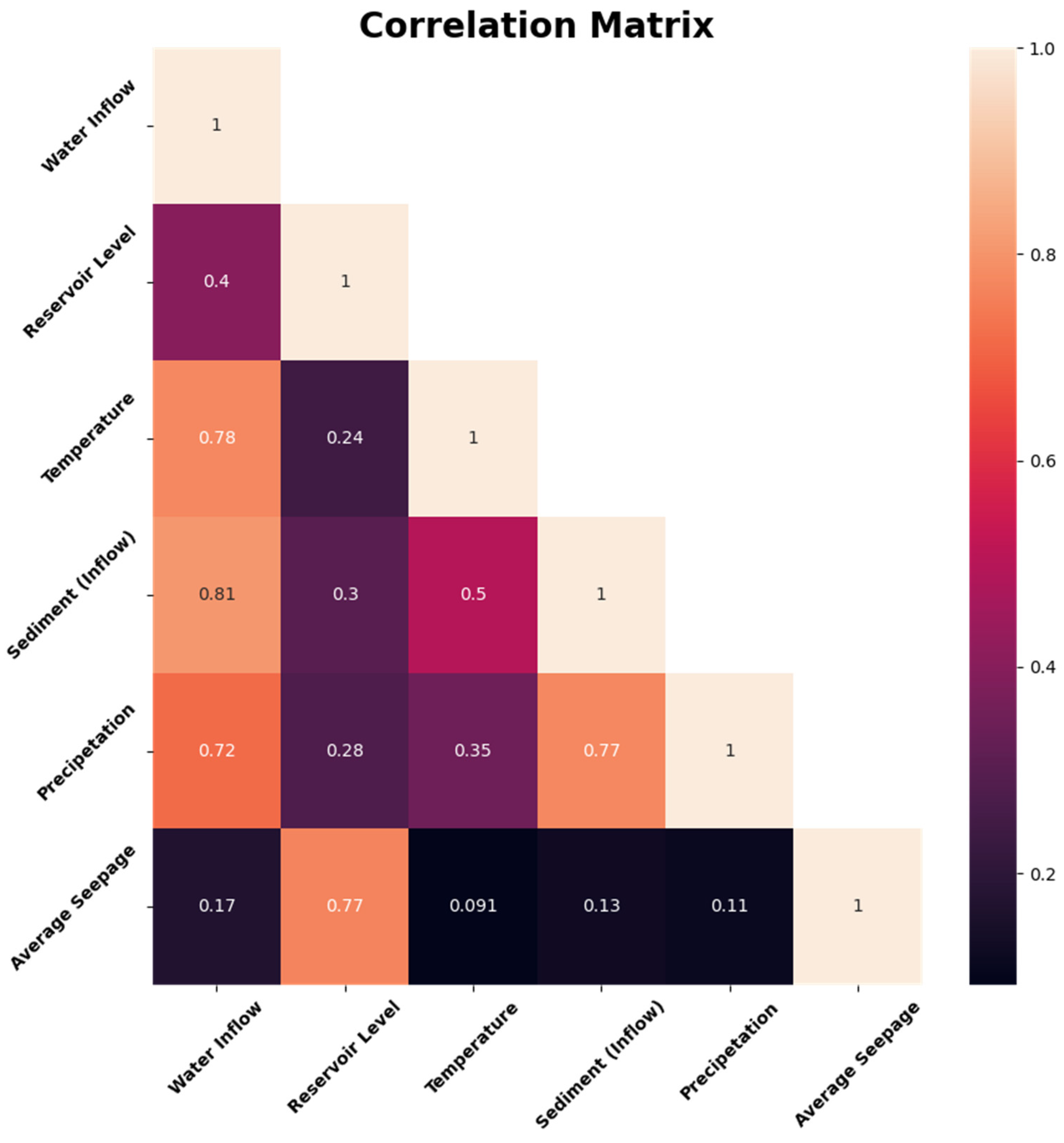
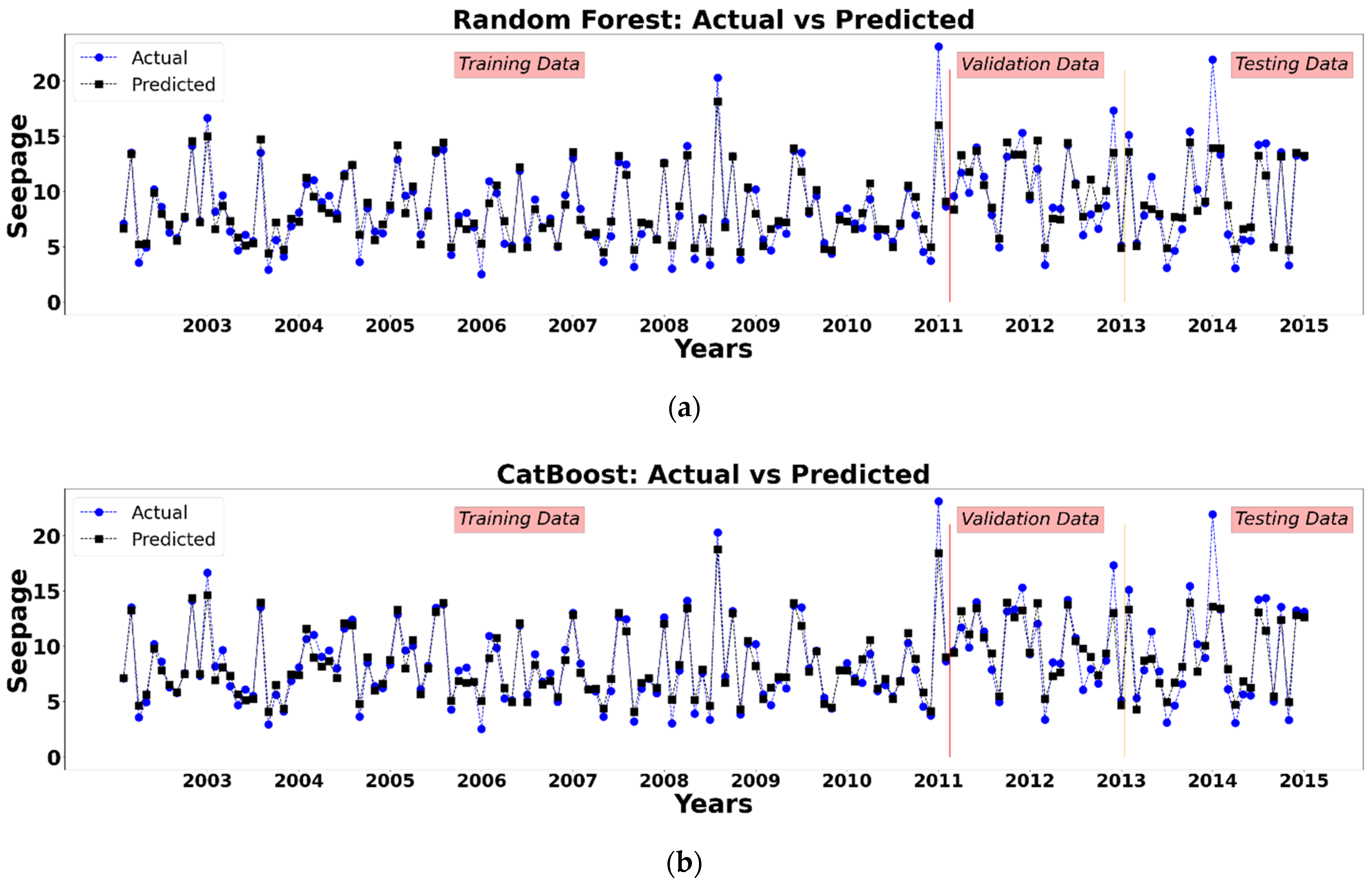
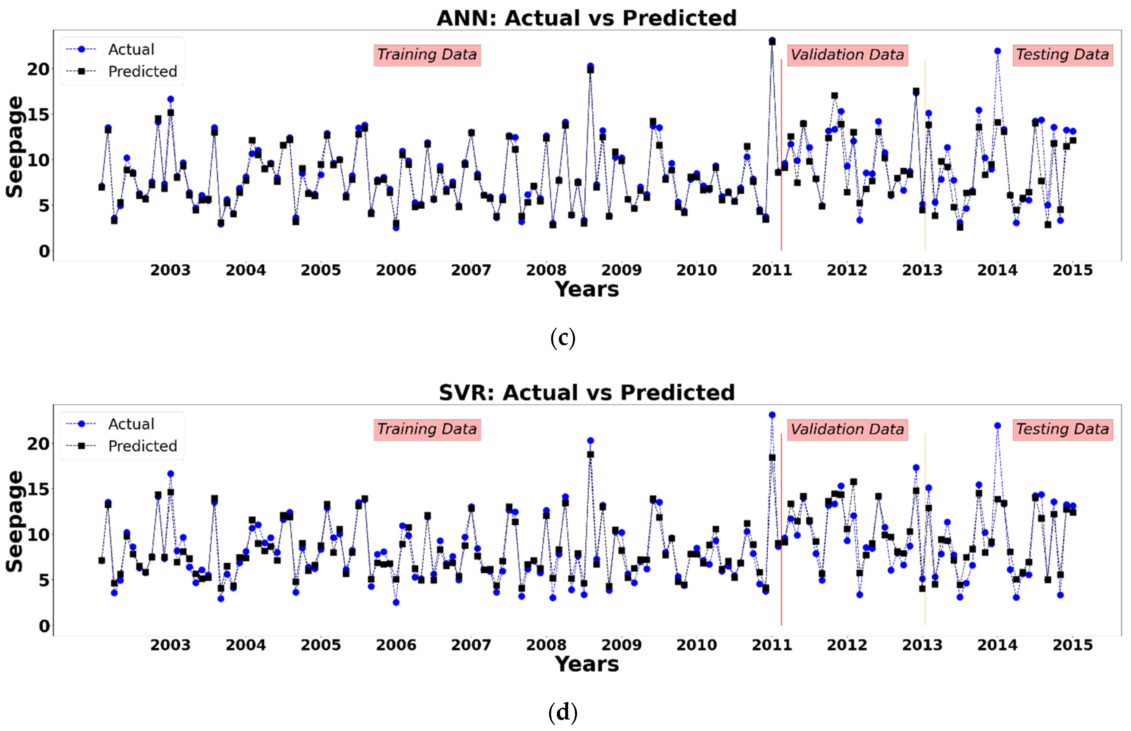
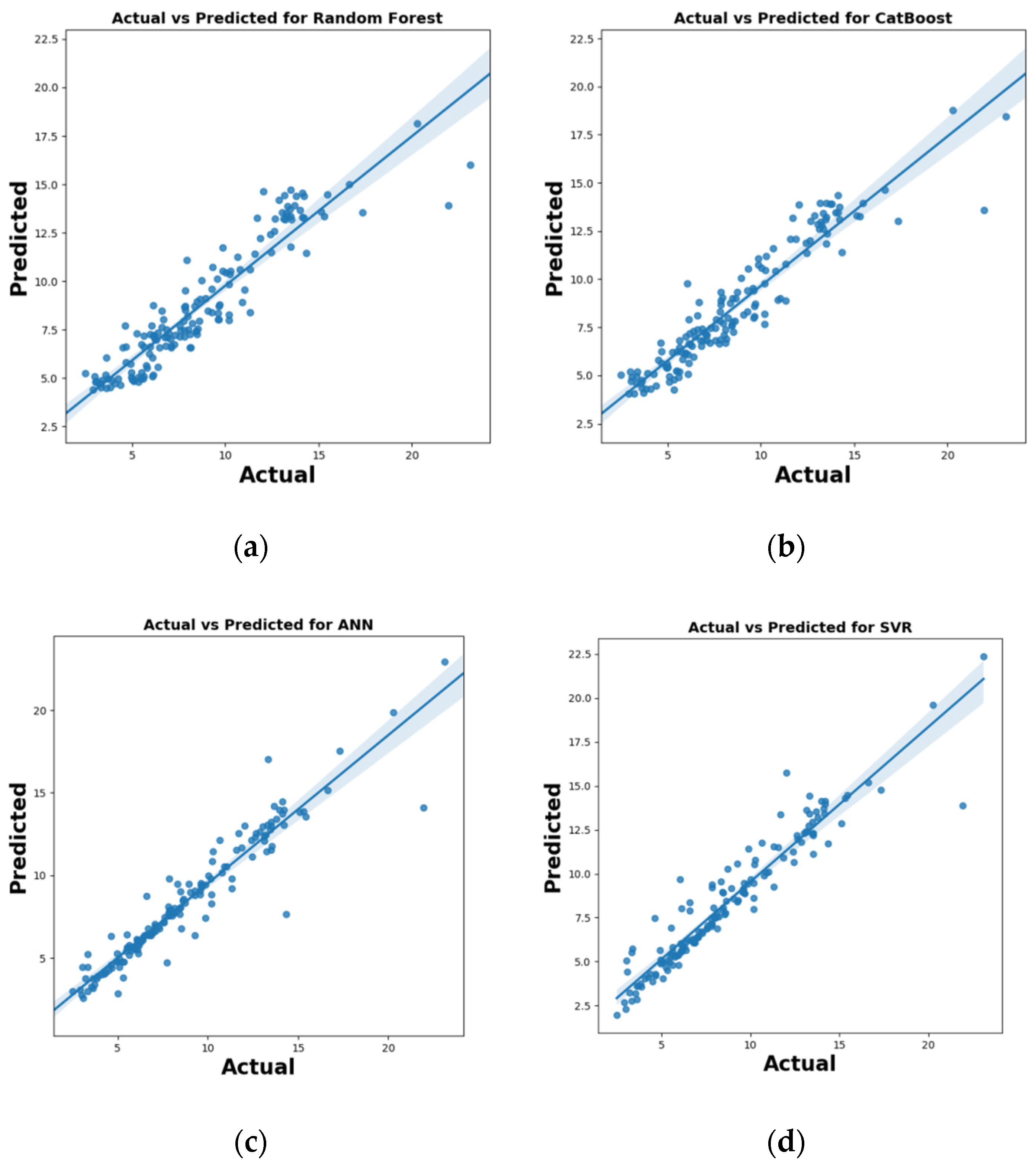
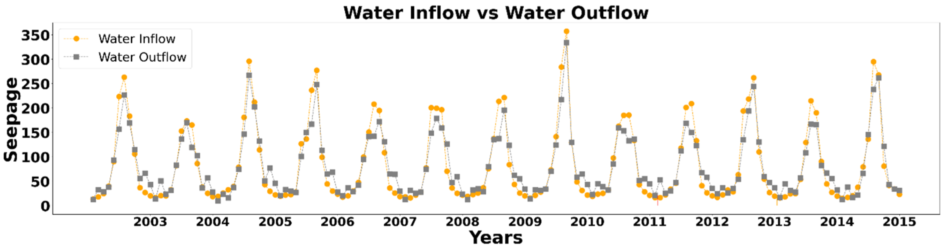
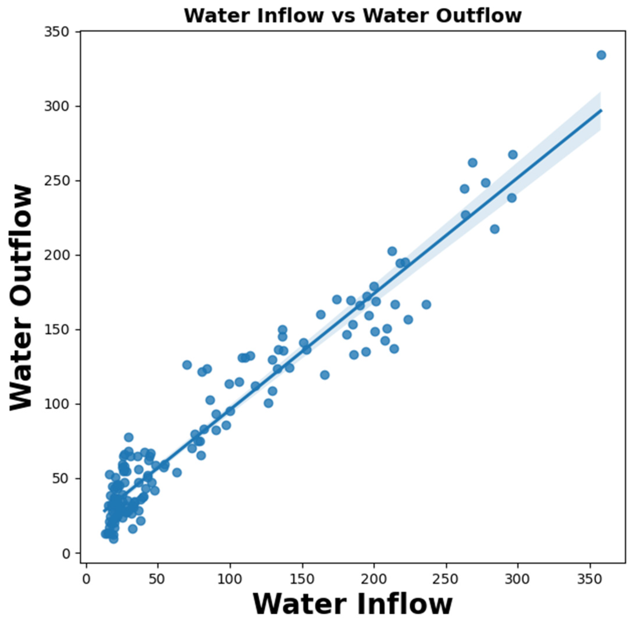
In this research, hydro-climatological parameters (Reservoir Level, Temperature, Sediment Inflow, Precipitation and Water Inflow and Water Outflow) were observed from 2003 to 2015 to understand their effect on the seepage in the Tarbela Dam, built on the Indus River of Pakistan. Firstly, four different machine learning algorithms, i.e., Random Forest, CatBoost, Support Vector Machine, and Artificial Neural Network, were used to model the relationship between the input variables and output to compare their performance in predicting the average seepage in the Tarbela Dam. Secondly, to explain the predictions of the machine learning models on the output, Shapley’s Additive ExPlanations (SHAP) algorithm (XAI: Model Explanation Algorithm) was used for each model to explain the sensitivity and effect of each parameter on the output variable (Average Seepage).

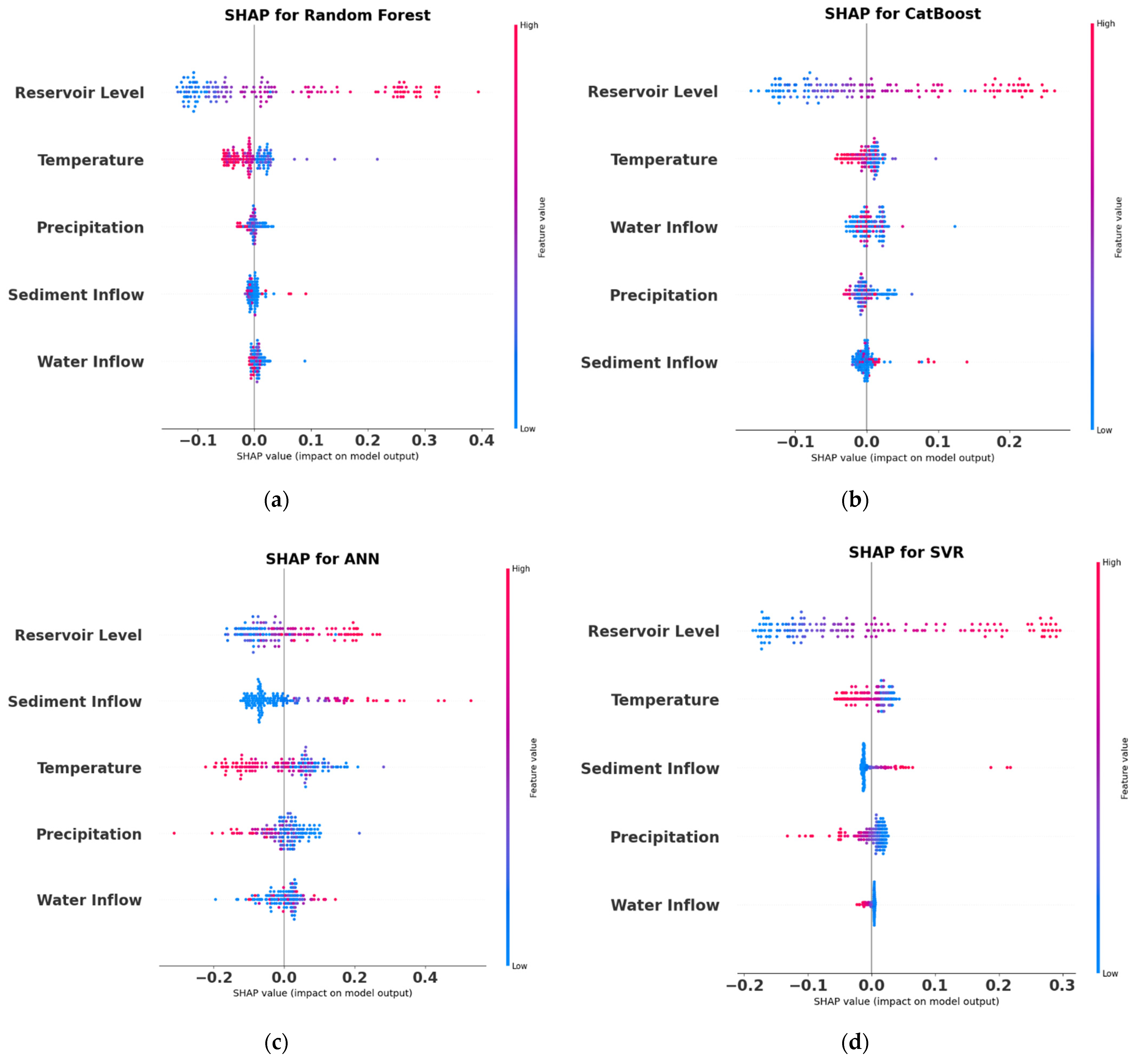
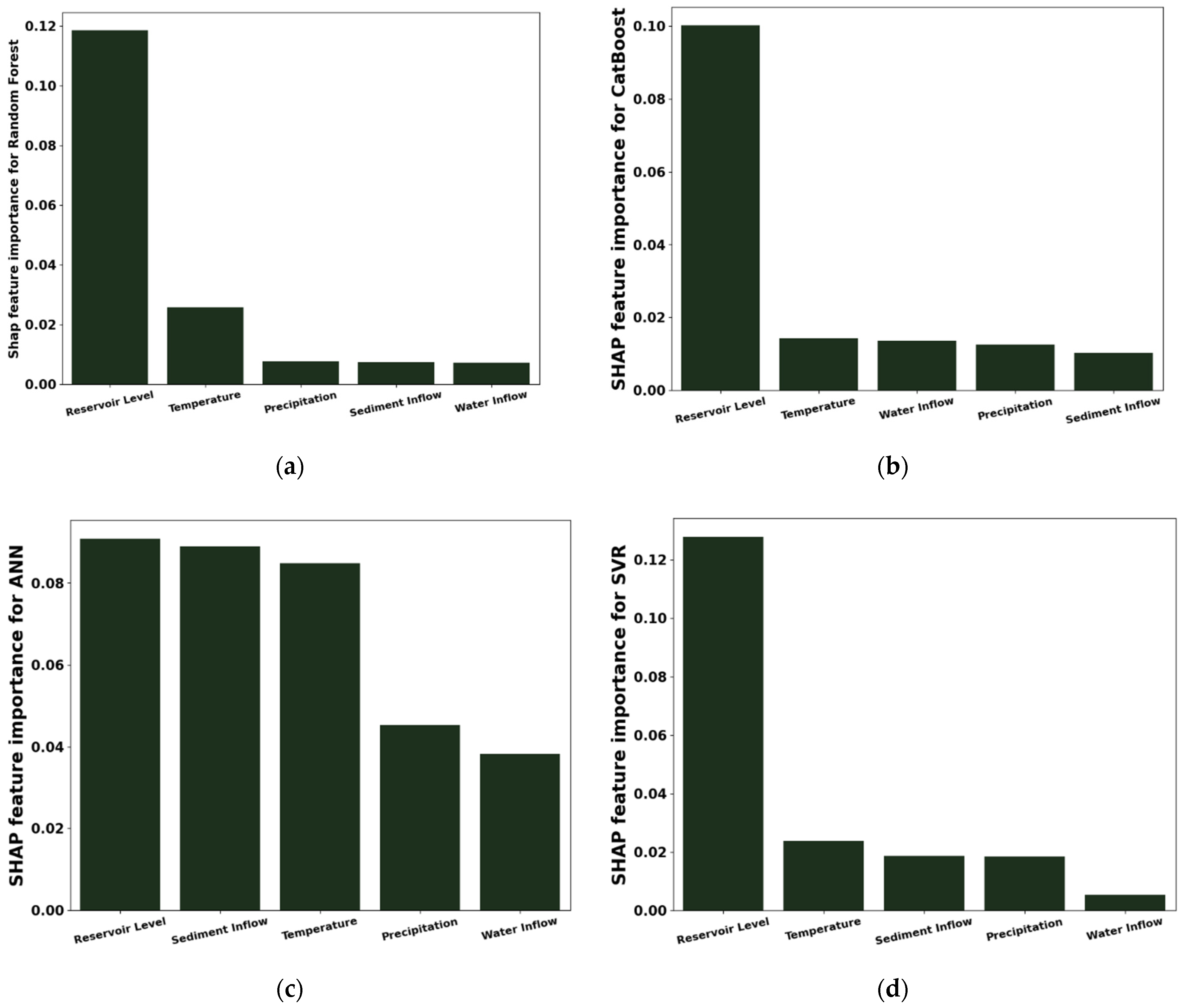
According to the findings of this study, the Random Forest, CatBoost, Support Vector Machine and Artificial Neural Network approach may be used to predict dam seepage based on hydro-climatological parameters in the Tarbela Dam. However, the CatBoost algorithm outperforms all the algorithms used for modeling by reporting the least RMSE and highest R² score during the training, testing and validation stage. The recommended algorithm is CatBoost for water resources management decision-making and policymaking and improved monitoring of seepage losses at Tarbela Dam using Artificial Intelligence-based modeling approaches. Furthermore, the SHAP algorithm for all the models, reports the Reservoir Level as the most important parameter affecting the average dam seepage. Increasing the Reservoir Level increases, the average dam seepage and vice versa.

The SHAP summary plots concluded that reservoir level directly impacts dam seepage compared to other parameters (water inflow, temperature, precipitation, sediment inflow). Sediment has a moderate positive effect on dam seepage compared to reservoir level. The SHAP values for water inflow shows a minimal effect compared to reservoir level and sediment inflow. It is also concluded that temperature and precipitation have a negative effect on dam seepage. Still, they play an important role in glacier melting and increasing water inflow from the source to the Tarbela Dam. The AI based modelling and SHAP feature importance highlights the role of the hydro-climatological variable on Tarbela Dam seepage which is an interesting analysis identifying the importance of reservoir level for dam seepage prediction.

A proper plan should be established in the coming decade to properly manage the droughts, floods and water inflow at downstream side of the dam. In addition, the model’s applicability will be superior in locations where data collecting is limited, in contrast with existing physical methods. Therefore, it is possible to increase sustainable water resource management through AI based analysis for seepage modelling in the dam. Water resources management, dam’s stability and safety should be a research priority in light of climate change. It is recommended to create a database of all relevant variables from the entire hydrological cycle and metrological data on dam sites for data collection, which will enable application of various AI based techniques to understand and improve dam seepage problems. Furthermore, this work could be extended by including more parameters, e.g., climatological parameters from region, induced seismicity data from dam, seismic events data such as earthquakes, soil parameters, and structural deformation such as crack and joints data in the dam for better AI based modelling, that will lead to better decision making, devising better policies to improve the dam stability and prevent against structural failures in the dam.

References

1. Adebiyi, J.A.; Olabisi, L.S.; Liu, L.; Jordan, D.J.E. Development; Sustainability. Water–food–energy–climate nexus and technology productivity: A Nigerian case study of organic leafy vegetable production. Environ. Dev. Sustain. 2021, 23, 6128–6147. [Google Scholar] [CrossRef]
2. Shen, D. The Strictest Water Resources Management Strategy and Its Three Red Lines. In Water Resources Management of the People’s Republic of China; Springer: Berlin/Heidelberg, Germany, 2021; pp. 253–274. [Google Scholar]
3. Demir, İ.; Kiliçkan, A. Renewable Energy Storage Methods. Int. Sci. J. 2018, 64, 103–107. [Google Scholar]
4. Rezaee, A.; Bozorg-Haddad, O.; Singh, V.P. Water and society. In Economical, Political, and Social Issues in Water Resources; Elsevier: Amsterdam, The Netherlands, 2021; pp. 257–271. [Google Scholar]
5. Kahlown, M.A.; Majeed, A. Water-resources situation in Pakistan: Challenges and future strategies. In Water Resources in the South: Present Scenario and Future Prospects; Commission on Science and Technology for Sustainable Development in the South: Islamabad, Pakistan, 2003; Volume 20, pp. 33–45. [Google Scholar]
6. Ishfaque, M.; Dai, Q.; Haq, N.u.; Jadoon, K.; Shahzad, S.M.; Janjuhah, H.T. Use of Recurrent Neural Network with Long Short-Term Memory for Seepage Prediction at Tarbela Dam, KP, Pakistan. Energies 2022, 15, 3123. [Google Scholar] [CrossRef]
7. Manivannan, S.; Thilagam, V.K.; Yaligar, R. Climate change impact on water resources in Indian river basins: A review. J. Soil Water Conserv. 2022, 21, 76–85. [Google Scholar] [CrossRef]
8. Lessard, J.; Hicks, D.M.; Snelder, T.H.; Arscott, D.B.; Larned, S.T.; Booker, D.; Suren, A.M. Dam design can impede adaptive management of environmental flows: A case study from the Opuha Dam, New Zealand. Environ. Manag. 2013, 51, 459–473. [Google Scholar] [CrossRef]
9. Rice, J.D.; Duncan, J.M. Findings of case histories on the long-term performance of seepage barriers in dams. J. Geotech. Geoenviron. Eng. 2010, 136, 2–15. [Google Scholar] [CrossRef]
10. Omofunmi, O.E.; Kolo, J.G.; Oladipo, A.S.; Diabana, P.D.; Ojo, A.S. A review on effects and control of seepage through earth-fill dam. Curr. J. Appl. Sci. Technol. 2017, 22, 1–11. [Google Scholar] [CrossRef]
11. Chen, G.; Jin, D.; Mao, J.; Gao, H.; Wang, Z.; Jing, L.; Li, Y.; Li, X. Seismic damage and behavior analysis of earth dams during the 2008 Wenchuan earthquake, China. Eng. Geol. 2014, 180, 99–129. [Google Scholar] [CrossRef]
12. Kayode, O.; Odukoya, A.M.; Adagunodo, T.; Adeniji, A. Monitoring of seepages around dams using geophysical methods: A brief review. IOP Conf. Ser. Earth Environ. Sci. 2018, 173, 012026. [Google Scholar] [CrossRef]
13. Zhao, E.; Jiang, Y. Seepage Evolution Model of the Fractured Rock Mass under High Seepage Pressure in Dam Foundation. Adv. Civ. Eng. 2021, 2021, 8832774. [Google Scholar] [CrossRef]
14. Himi, M.; Casado, I.; Sendros, A.; Lovera, R.; Rivero, L.; Casas, A. Assessing preferential seepage and monitoring mortar injection through an earthen dam settled over a gypsiferous substrate using combined geophysical methods. Eng. Geol. 2018, 246, 212–221. [Google Scholar] [CrossRef]
15. Coulibaly, Y.; Belem, T.; Cheng, L. Numerical analysis and geophysical monitoring for stability assessment of the Northwest tailings dam at Westwood Mine. Int. J. Min. Sci. Technol. 2017, 27, 701–710. [Google Scholar] [CrossRef]
16. Dahlin, T. Geoelectrical monitoring of embankment dams for detection of anomalous seepage and internal erosion—Experiences and work in progress in Sweden. In Proceedings of the Fifth International Conference on Engineering Geophysics (ICEG), Al Ain, United Arab Emirates, 21–24 October 2019; pp. 207–210. [Google Scholar]
17. Komasi, M.; Beiranvand, B. Seepage and Stability Analysis of the Eyvashan Earth Dam under Drawdown Conditions. Civ. Eng. Infrastruct. J. 2021, 54, 205–223. [Google Scholar]
18. Fang, C.; Duan, Y. Statistical analysis of dam-break incidents and its cautions. Yangtze River 2010, 41, 97–100. [Google Scholar]
19. Jiang, X.; Wei, Y.; Wu, L.; Hu, K.; Zhu, Z.; Zou, Z.; Xiao, W. Laboratory experiments on failure characteristics of non-cohesive sediment natural dam in progressive failure mode. Environ. Earth Sci. 2019, 78, 538. [Google Scholar] [CrossRef]
20. Liu, L.-L.; Cheng, Y.-M.; Jiang, S.-H.; Zhang, S.-H.; Wang, X.-M.; Wu, Z.-H. Effects of spatial autocorrelation structure of permeability on seepage through an embankment on a soil foundation. Comput. Geotech. 2017, 87, 62–75. [Google Scholar] [CrossRef]
21. Adamo, N.; Al-Ansari, N.; Sissakian, V.; Laue, J.; Knutsson, S.; Engineering, G. Geophysical Methods and their Applications in Dam Safety Monitoring. J. Earth Sci. Geotech. Eng. 2021, 11, 291–345. [Google Scholar] [CrossRef]
22. Cui, H.D.; Chen, L.; Wang, J.L.; Zhang, W. Study on anti-seepage treatment and seepage control effect of core dam foundation curtain of the fault fracture zone in Xinjiang province. IOP Conf. Ser. Earth Environ. Sci. 2020, 643, 012108. [Google Scholar] [CrossRef]
23. Zhang, C.; Chai, J.; Cao, J.; Xu, Z.; Qin, Y.; Lv, Z. Numerical Simulation of Seepage and Stability of Tailings Dams: A Case Study in Lixi, China. Water 2020, 12, 742. [Google Scholar] [CrossRef]
24. Coppens, J.; Trolle, D.; Jeppesen, E.; Beklioğlu, M. The impact of climate change on a Mediterranean shallow lake: Insights based on catchment and lake modelling. Reg. Environ. Chang. 2020, 20, 62. [Google Scholar] [CrossRef]
25. Xu, S.; Chen, C.; Xu, F.; Li, J.; Zhang, Z.; Xu, T.; Zhu, L. Modeling Analysis of the Upper Limit Water Level Mechanism in the Upstream Reservoir of a Dam Embankment. Adv. Civ. Eng. 2020, 2020, 8850681. [Google Scholar] [CrossRef]
26. Beiranvand, B.; Komasi, M. An Investigation on performance of the cut off wall and numerical analysis of seepage and pore water pressure of Eyvashan earth dam. Iran. J. Sci. Technol. Trans. Civ. Eng. 2021, 45, 1723–1736. [Google Scholar] [CrossRef]
27. Wang, T.; Chen, J.; Li, P.; Yin, Y.; Shen, C. Natural tracing for concentrated leakage detection in a rockfill dam. Eng. Geol. 2019, 249, 1–12. [Google Scholar] [CrossRef]
28. Al-Fares, W. Application of electrical resistivity tomography technique for characterizing leakage problem in Abu Baara earth dam, Syria. Int. J. Geophys. 2014, 2014, 368128. [Google Scholar] [CrossRef]
29. Neyamadpour, A.; Abbasinia, M. Application of electrical resistivity tomography technique to delineate a structural failure in an embankment dam: Southwest of Iran. Arab. J. Geosci. 2019, 12, 420. [Google Scholar] [CrossRef]
30. Okpoli, C.; Tijani, R. Electromagnetic profiling of Owena Dam, Southwestern Nigeria, using very-low-frequency radio fields. Mater. Geoenviron. 2016, 63, 237–250. [Google Scholar] [CrossRef]
31. Ahmed, A.S.; Revil, A.; Bolève, A.; Steck, B.; Vergniault, C.; Courivaud, J.; Jougnot, D.; Abbas, M. Determination of the permeability of seepage flow paths in dams from self-potential measurements. Eng. Geol. 2020, 268, 105514. [Google Scholar] [CrossRef]
32. Li, X.; Fan, L.; Huang, H.; Hao, J.; Li, M. Application of Ground Penetrating Radar in Leakage Detection of Concrete Face Rockfill Dam. IOP Conf. Ser. Earth Environ. Sci. 2018, 189, 022044. [Google Scholar] [CrossRef]
33. Raji, W.O.; Aluko, K.O. Investigating the cause of excessive seepage in a dam foundation using seismic and electrical surveys—A case study of Asa Dam, West Africa. Bull. Eng. Geol. Environ. 2021, 80, 6445–6455. [Google Scholar] [CrossRef]
34. Al-Janabi, A.M.S.; Ghazali, A.H.; Ghazaw, Y.M.; Afan, H.A.; Al-Ansari, N.; Yaseen, Z.M. Experimental and numerical analysis for earth-fill dam seepage. Sustainability 2020, 12, 2490. [Google Scholar] [CrossRef]
35. Li, G.C.; Desai, C.S. Stress and seepage analysis of earth dams. J. Geotech. Eng. 1983, 109, 946–960. [Google Scholar] [CrossRef]
36. Finn, W.D.L. Finite-element analysis of seepage through dams. J. Soil Mech. Found. Div. 1967, 93, 41–48. [Google Scholar] [CrossRef]
37. Neuman, S.P.; Witherspoon, P.A. Finite element method of analyzing steady seepage with a free surface. Water Resour. Res. 1970, 6, 889–897. [Google Scholar] [CrossRef]
38. Bathe, K.J.; Khoshgoftaar, M.R. Finite element free surface seepage analysis without mesh iteration. Int. J. Numer. Anal. Methods Geomech. 1979, 3, 13–22. [Google Scholar] [CrossRef]
39. Ng, A.K.; Small, J.C. A case study of hydraulic fracturing using finite element methods. Can. Geotech. J. 1999, 36, 861–875. [Google Scholar] [CrossRef]
40. Callari, C.; Abati, A. Finite element methods for unsaturated porous solids and their application to dam engineering problems. Comput. Struct. 2009, 87, 485–501. [Google Scholar] [CrossRef]
41. Kazemzadeh-Parsi, M.J.; Daneshmand, F. Unconfined seepage analysis in earth dams using smoothed fixed grid finite element method. Int. J. Numer. Anal. Methods Geomech. 2012, 36, 780–797. [Google Scholar] [CrossRef]
42. Olonade, K.A.; Agbede, O.A. A study of seepage through oba dam using finite element method. Civ. Environ. Res. 2013, 3, 53–60. [Google Scholar]
43. Athani, S.S.; Shivamanth; Solanki, C.; Dodagoudar, G. Seepage and stability analyses of earth dam using finite element method. Aquat. Procedia 2015, 4, 876–883. [Google Scholar] [CrossRef]
44. Jamel, A.A.J. Analysis and estimation of seepage through homogenous earth dam without filter. Diyala J. Eng. Sci. 2016, 9, 38–49. [Google Scholar] [CrossRef]
45. Khassaf, S.I.; Madhloom, A.M. Effect of impervious core on seepage through zoned earth dam (case study: Khassa Chai dam). Int. J. Sci. Eng. Res. 2017, 8, 1053–1064. [Google Scholar]
46. Liu, C.; Shen, Z.; Gan, L.; Xu, L.; Zhang, K.; Jin, T. The seepage and stability performance assessment of a new drainage system to increase the height of a tailings dam. Appl. Sci. 2018, 8, 1840. [Google Scholar] [CrossRef]
47. Athani, S.S.; Solanki, C.; Dodagoudar, G.R.; Shukla, S.K. Finite-element analysis of strains in seepage barriers of the earth dam. Dams Reserv. 2019, 29, 87–96. [Google Scholar] [CrossRef]
48. Al-Nedawi, N.M. Finite element analysis of seepage for Hemrin earth dam using Geo-Studio software. Diyala J. Eng. Sci. 2020, 13, 66–76. [Google Scholar] [CrossRef]
49. Bai, C.; Chai, J.; Xu, Z.; Qin, Y. Numerical Simulation of Drainage Holes and Performance Evaluation of the Seepage Control of Gravity Dam: A Case Study of Heihe Reservoir in China. Arab. J. Sci. Eng. 2021, 47, 4801–4819. [Google Scholar] [CrossRef]
50. Tarinejad, R.; Alizadeh-Arasi, O.; Isari, M.; Foumani, R.S. Investigation of Sabalan Earth Dam Settlement at First Filling by Finite Difference Method. Transp. Infrastruct. Geotechnol. 2021, 8, 473–490. [Google Scholar] [CrossRef]
51. Aghdam, A.T.; Salmasi, F.; Abraham, J.; Arvanaghi, H. Effect of Drain Pipes on Uplift Force and Exit Hydraulic Gradient and the Design of Gravity Dams Using the Finite Element Method. Geotech. Geol. Eng. 2021, 39, 3383–3399. [Google Scholar] [CrossRef]
52. Yuan, S.; Zhong, H. Three dimensional analysis of unconfined seepage in earth dams by the weak form quadrature element method. J. Hydrol. 2016, 533, 403–411. [Google Scholar] [CrossRef]
53. Jing, T.; Yongbiao, L. Penalty function element free method to solve complex seepage field of earth fill dam. IERI Procedia 2012, 1, 117–123. [Google Scholar] [CrossRef]
54. Fallah, A.; Jabbari, E.; Babaee, R. Development of the Kansa method for solving seepage problems using a new algorithm for the shape parameter optimization. Comput. Math. Appl. 2019, 77, 815–829. [Google Scholar] [CrossRef]
55. Sharghi, E.; Nourani, V.; Behfar, N. Implementation of Data Jittering Technique for Seepage Analysis of Earth fill Dam Using Ensemble of AI Models. Water Soil Sci. 2020, 30, 29–41. [Google Scholar]
56. Sharghi, E.; Nourani, V.; Behfar, N. Earthfill dam seepage analysis using ensemble artificial intelligence based modeling. J. Hydroinform. 2018, 20, 1071–1084. [Google Scholar] [CrossRef]
57. Rehamnia, I.; Benlaoukli, B.; Heddam, S. Modeling of Seepage Flow Through Concrete Face Rockfill and Embankment Dams Using Three Heuristic Artificial Intelligence Approaches: A Comparative Study. Environ. Process. 2020, 7, 367–381. [Google Scholar] [CrossRef]
58. Alocén, P.; Fernández-Centeno, M.Á.; Toledo, M.Á. Prediction of Concrete Dam Deformation through the Combination of Machine Learning Models. Water 2022, 14, 1133. [Google Scholar] [CrossRef]
59. Ibañez, S.C.; Dajac, C.V.G.; Liponhay, M.P.; Legara, E.F.T.; Esteban, J.M.H.; Monterola, C.P. Forecasting reservoir water levels using deep neural networks: A case study of Angat Dam in the Philippines. Water 2021, 14, 34. [Google Scholar] [CrossRef]
60. Jiang, D.; Xu, Y.; Lu, Y.; Gao, J.; Wang, K. Forecasting Water Temperature in Cascade Reservoir Operation-Influenced River with Machine Learning Models. Water 2022, 14, 2146. [Google Scholar] [CrossRef]
61. Choi, H.S.; Kim, J.H.; Lee, E.H.; Yoon, S.-K. Development of a Revised Multi-Layer Perceptron Model for Dam Inflow Prediction. Water 2022, 14, 1878. [Google Scholar] [CrossRef]
62. Zhang, X.; Chen, X.; Li, J. Improving dam seepage prediction using back-propagation neural network and genetic algorithm. Math. Probl. Eng. 2020, 2020, 1404295. [Google Scholar] [CrossRef]
63. Nouri, M.; Salmasi, F. Predicting Seepage of Earth Dams using Artificial Intelligence Techniques. J. Irrig. Sci. Eng. 2019, 42, 83–97. [Google Scholar]
64. Nourani, V.; Sharghi, E.; Aminfar, M.H. Integrated ANN model for earthfill dams seepage analysis: Sattarkhan Dam in Iran. Artif. Intell. Res. 2012, 1, 22–37. [Google Scholar] [CrossRef]
65. Yaseen, Z.M.; Naghshara, S.; Salih, S.Q.; Kim, S.; Malik, A.; Ghorbani, M.A. Lake water level modeling using newly developed hybrid data intelligence model. Theor. Appl. Climatol. 2020, 141, 1285–1300. [Google Scholar] [CrossRef]
66. Parsaie, A.; Haghiabi, A.H.; Latif, S.D.; Tripathi, R.P. Predictive modelling of piezometric head and seepage discharge in earth dam using soft computational models. Environ. Sci. Pollut. Res. 2021, 28, 60842–60856. [Google Scholar] [CrossRef] [PubMed]
67. Sani, H.; Roushangar, K.; Ghasempour, R. Comparative study of the performance of finite element method and evolutionary model in seepage discharge predicting from the body of an earth dam. Civ. Infrastruct. Res. 2019, 4, 1–15. [Google Scholar]
68. Roushangar, K.; Garekhani, S.; Alizadeh, F. Forecasting daily seepage discharge of an earth dam using wavelet–mutual information–Gaussian process regression approaches. Geotech. Geol. Eng. 2016, 34, 1313–1326. [Google Scholar] [CrossRef]
69. Chen, S.; Gu, C.; Lin, C.; Wang, Y.; Hariri-Ardebili, M.A. Prediction, monitoring, and interpretation of dam leakage flow via adaptative kernel extreme learning machine. Measurement 2020, 166, 108161. [Google Scholar] [CrossRef]
70. Zhao, M.; Jiang, H.; Chen, S.; Bie, Y. Prediction of Seepage Pressure Based on Memory Cells and Significance Analysis of Influencing Factors. Complexity 2021, 2021, 5576148. [Google Scholar] [CrossRef]
71. El Bilali, A.; Moukhliss, M.; Taleb, A.; Nafii, A.; Alabjah, B.; Brouziyne, Y.; Mazigh, N.; Teznine, K.; Mhamed, M. Predicting daily pore water pressure in embankment dam: Empowering Machine Learning-based modeling. Environ. Sci. Pollut. Res. 2022, 29, 47382–47398. [Google Scholar] [CrossRef]
72. Rehamnia, I.; Benlaoukli, B.; Jamei, M.; Karbasi, M.; Malik, A. Simulation of seepage flow through embankment dam by using a novel extended Kalman filter based neural network paradigm: Case study of Fontaine Gazelles Dam, Algeria. Measurement 2021, 176, 109219. [Google Scholar] [CrossRef]
73. Khan, N.M.; Tingsanchali, T. Optimization and simulation of reservoir operation with sediment evacuation: A case study of the Tarbela Dam, Pakistan. Hydrol. Process. 2009, 23, 730–747. [Google Scholar] [CrossRef]
74. Rafique, A.; Burian, S.; Hassan, D.; Bano, R. Analysis of Operational Changes of Tarbela Reservoir to Improve the Water Supply, Hydropower Generation, and Flood Control Objectives. Sustainability 2020, 12, 7822. [Google Scholar] [CrossRef]
75. Roca, M. Tarbela Dam in Pakistan. Case study of reservoir sedimentation. In River Flow 2012: Proceedings of the International Conference on Fluvial Hydraulics, San José, Costa Rica, 5–7 September 2012; HR Wallingford: Wallingford, UK, 2012. [Google Scholar]
76. Murphy, K.P. Probabilistic Machine Learning: An Introduction; MIT Press: Cambridge, MA, USA, 2022. [Google Scholar]
77. Salem, H.; Kabeel, A.; El-Said, E.M.; Elzeki, O.M. Predictive modelling for solar power-driven hybrid desalination system using artificial neural network regression with Adam optimization. Desalination 2022, 522, 115411. [Google Scholar] [CrossRef]
78. Karami, H.; DadrasAjirlou, Y.; Jun, C.; Bateni, S.M.; Band, S.S.; Mosavi, A.; Moslehpour, M.; Chau, K.-W. A novel approach for estimation of sediment load in Dam reservoir with hybrid intelligent algorithms. Front. Environ. Sci. 2022, 165. [Google Scholar] [CrossRef]
79. Breiman, L. Random forests. Mach. Learn. 2001, 45, 5–32. [Google Scholar] [CrossRef]
80. Were, K.; Bui, D.T.; Dick, Ø.B.; Singh, B.R. A comparative assessment of support vector regression, artificial neural networks, and random forests for predicting and mapping soil organic carbon stocks across an Afromontane landscape. Ecol. Indic. 2015, 52, 394–403. [Google Scholar] [CrossRef]
81. Oliveira, S.; Oehler, F.; San-Miguel-Ayanz, J.; Camia, A.; Pereira, J.M. Modeling spatial patterns of fire occurrence in Mediterranean Europe using Multiple Regression and Random Forest. For. Ecol. Manag. 2012, 275, 117–129. [Google Scholar] [CrossRef]
82. Naghibi, S.A.; Ahmadi, K.; Daneshi, A. Application of support vector machine, random forest, and genetic algorithm optimized random forest models in groundwater potential mapping. Water Resour. Manag. 2017, 31, 2761–2775. [Google Scholar] [CrossRef]
83. Al-Abadi, A.M.; Shahid, S. Spatial mapping of artesian zone at Iraqi southern desert using a GIS-based random forest machine learning model. Modeling Earth Syst. Environ. 2016, 2, 96. [Google Scholar] [CrossRef]
84. Huang, N.; Lu, G.; Xu, D. A permutation importance-based feature selection method for short-term electricity load forecasting using random forest. Energies 2016, 9, 767. [Google Scholar] [CrossRef]
85. Vapnik, V.N. The Nature of Statistical Learning; Springer: Berlin/Heidelberg, Germany, 1995. [Google Scholar]
86. Ke, G.; Meng, Q.; Finley, T.; Wang, T.; Chen, W.; Ma, W.; Ye, Q.; Liu, T.-Y. Lightgbm: A highly efficient gradient boosting decision tree. Adv. Neural Inf. Process. Syst. 2017, 30, 3149–3157. [Google Scholar]
87. Dhieb, N.; Ghazzai, H.; Besbes, H.; Massoud, Y. Extreme gradient boosting machine learning algorithm for safe auto insurance operations. In Proceedings of the 2019 IEEE International Conference on Vehicular Electronics and Safety (ICVES), Cairo, Egypt, 4–6 September 2019; pp. 1–5. [Google Scholar]
88. Dorogush, A.V.; Ershov, V.; Gulin, A. CatBoost: Gradient boosting with categorical features support. arXiv 2018, arXiv:1810.11363. [Google Scholar]
89. Prokhorenkova, L.; Gusev, G.; Vorobev, A.; Dorogush, A.V.; Gulin, A. CatBoost: Unbiased boosting with categorical features. Adv. Neural Inf. Process. Syst. 2018, 31. [Google Scholar] [CrossRef]
90. Dorogush, A.V.; Gulin, A.; Gusev, G.; Kazeev, N.; Prokhorenkova, L.O.; Vorobev, A. Fighting biases with dynamic boosting. arXiv 2017, arXiv:1706.09516. [Google Scholar]
91. Lundberg, S.M.; Lee, S.-I. A unified approach to interpreting model predictions. Adv. Neural Inf. Process. Syst. 2017, 30. [Google Scholar] [CrossRef]
92. Bataineh, M.; Steenhard, D.; Singh, H. Feature Impact for Prediction Explanation. In Proceedings of the ICDM (Posters), New York, NY, USA, 17–21 July 2019; pp. 160–167. [Google Scholar]
93. Tallón-Ballesteros, A.; Chen, C. Explainable AI: Using Shapley value to explain complex anomaly detection ML-based systems. In Machine Learning and Artificial Intelligence; IOS Press: Amsterdam, The Netherlands, 2020; Volume 332, p. 152. [Google Scholar]
94. Wieland, R.; Lakes, T.; Nendel, C. Using SHAP to interpret XGBoost predictions of grassland degradation in Xilingol, China. Geosci. Model Dev. Discuss. 2020, 2020, 1–28. [Google Scholar]
95. Štrumbelj, E.; Kononenko, I. Explaining prediction models and individual predictions with feature contributions. Knowl. Inf. Syst. 2014, 41, 647–665. [Google Scholar] [CrossRef]
96. Legates, D.R.; McCabe Jr, G.J. Evaluating the use of "goodness-of-fit" measures in hydrologic and hydroclimatic model validation. Water Resour. Res. 1999, 35, 233–241. [Google Scholar] [CrossRef]
97. Moghimi, M.M.; Zarei, A.R. Evaluating performance and applicability of several drought indices in arid regions. Asia-Pac. J. Atmos. Sci. 2021, 57, 645–661. [Google Scholar] [CrossRef]
98. Akhter, M. Dams as a climate change adaptation strategy: Geopolitical implications for Pakistan. Strateg. Anal. 2015, 39, 744–748. [Google Scholar] [CrossRef]
99. Hewitt, K.; Wake, C.P.; Young, G.; David, C. Hydrological investigations at Biafo Glacier, Karakoram Range, Himalaya; An important source of water for the Indus River. Ann. Glaciol. 1989, 13, 103–108. [Google Scholar] [CrossRef]
100. Yaseen, M.; Latif, Y.; Waseem, M.; Leta, M.K.; Abbas, S.; Akram Bhatti, H. Contemporary Trends in High and Low River Flows in Upper Indus Basin, Pakistan. Water 2022, 14, 337. [Google Scholar] [CrossRef]
Figure 1. Satellite image of Tarbela Dam site used for this study. (A) Tarbela dam satellite overview, (B) Tarbela power house, (C) Tarbela dam main abutment.
Water 14 02598 g001
Figure 2. Research flow chart for Machine Learning Models.
Water 14 02598 g002
Figure 3. Artificial Neural Network (ANN) Architecture for hydro-climatological variable prediction schema.
Water 14 02598 g003
Figure 4. The architecture of the random forest algorithm.
Water 14 02598 g004
Figure 5. CatBoost (CB) Algorithm Structure.
Water 14 02598 g005
Figure 6. Correlation Matrix for hydro-Metrological variables.
Water 14 02598 g006
Figure 7. Actual vs. Predicted Average Seepage from Machine learning (ML) Models.
Water 14 02598 g007aWater 14 02598 g007b
Figure 8. Comparison of Average seepage (Actual vs. Predicted) for (a) RF, (b) CatBoost, (c) ANN and (d) SVM Models.
Water 14 02598 g008
Figure 9. Comparison of Water Inflow and Outflow in Tarbela Dam.
Water 14 02598 g009
Figure 10. Regression Plot between water inflow and water outflow.
Water 14 02598 g010
Figure 11. SHAP value summary of Hydro-Climatological Parameters for each model.
Water 14 02598 g011
Figure 12. SHAP feature importance plots (a). Random forest (b). CatBoost (c). ANN (d). SVR.
Water 14 02598 g012