
Comparison of the Calibrated Objective Functions for Low Flow Simulation in a Semi-Arid Catchment

1
State Key Laboratory of Eco-Hydraulics in Northwest Arid Region, Xi’an University of Technology, Xi’an 710048, China
2
Shandong Xinhui Construction Group Co., Ltd., Dongying 257091, China
3
State Key Laboratory of Environmental Criteria and Risk Assessment, Chinese Research Academy of Environmental Sciences, Beijing 100012, China
4
Tianjin Academy of Eco-Environmental Sciences, Tianjin 300191, China
*
Author to whom correspondence should be addressed.
Water 2022, 14(17), 2591; https://doi.org/10.3390/w14172591
Submission received: 22 July 2022
/
Revised: 18 August 2022
/
Accepted: 19 August 2022
/
Published: 23 August 2022
(This article belongs to the Special Issue Advanced Hydrologic Modeling in Watershed Scales)
Abstract
:Low flow simulation by hydrological models is a common solution in water research and application. However, knowledge about the influence of the objective functions is limited in relatively arid regions. This study aims to increase insight into the difference between the calibrated objective functions by evaluating eight objectives in three different classes (single objectives: KGE(log(Q)) and KGE(1/Q); multi objectives: KGE(Q)+KGE(log(Q)), KGE(Q)+KGE(1/Q), KGE(Qsort)+KGE(log(Qsort)) and KGE(Qsort)+KGE(1/Qsort); Split objectives: split KGE(Q) and split (KGE(Q)+KGE(1/Q))) in Bahe, a semi-arid basin in China. The calibrated model is Xin An Jiang, and the evaluation is repeated under varied climates. The results show a clear difference between objective functions for low flows, and the mean of KGE and logarithmic transformed-based KGE in time series (KGE(Q)+KGE(log(Q))) presents the best compromise between the estimation for low flows and general simulation. In addition, the applications of the inverse transformed-based KGE (KGE(1/Q)) and the Flow Duration Curve-based series (Qsort) in objectives are not suggested.
1. Introduction
Low flow research plays a significant role in water management, such as aquatic ecosystems, irrigation, water supply, and hydroelectricity [1,2]. Applying hydrological models to low flow analysis is essential, especially for basins lacking discharge data [3]. However, hydrological models have simplified the water cycling processes and include some model parameters that cannot be directly measured [4]. Therefore, before applying the model in the interested regions, model calibration is essential to optimize the model parameters [5]. Due to the changing climate, growing scientific efforts to assess hydrological changes for future scenarios have been made. Aiming to reduce the uncertainty of future predictions, generating well-calibrated models is imperative [6].
Model calibration is the process of identifying a suitable model parameter set to minimize the difference between the simulated and observed values, represented by the objective function [7]. Thus, an excellent objective function is always the backbone of a satisfactory scientific outcome. To understand the influence of objective functions and improve the model simulation, considerable research has been carried out in recent decades (e.g., [8,9,10,11]). The most critical improvement is replacing the single objective with multi-objective (e.g., [12,13]), making the multi-objective calibration widely used in water resource applications, especially for hydrological simulations [14]. Efstratiadis and Koutsoyiannis [9] reviewed different case studies about multi-objective applications in hydrology and found that the multi-objective approach improved the identifiability of parameters in complex parameterization.
Even though a significant number of studies have applied various multi-objective functions in hydrological model calibration, studies focusing on low flow analysis are limited. Shafii and De Smedt [15] calibrated the WetSpa model by combining the normal and log-transformed Nash–Sutcliffe Efficiency (NSE) as the objective function and found that it is possible to find a compromise with equal attention to both high-flows and low-flows. Kim [16] also applied the normal and log-transformed NSE in the objective function to emphasize high and low flow in a hydrograph and concluded that it worked better. Garcia et al. [3] conducted a comprehensive evaluation, particularly on low flow simulations with different objective functions in hundreds of French basins but applied the inverse transformation to make the low flow sensitive to the objective functions. Their result suggested that the combination between normal and inverse transformed Kling Gupta Efficiency (KGE) is recommended. Apart from the transformed format of objective functions based on time series, studies including the hydrological signatures in the objective function are increasing. According to the comparison between the time series-based and Flow Duration Curve (FDC)-based transformed format of objective functions, Garcia et al. [3] found using FDC based transformation is worse than the time series-based objective function for low flow indices simulation. At the same time, Lombardi et al. [17] deduced that including the match of the FDC statistic in the calibration outperformed the time domain calibration on an excellent reproduction of the low-to-average flow quantiles, based on 52 Italian catchments. Consistent with Lombardi et al. [17], Chilkoti et al. [14] found the inclusion of FDC-based signatures in objective functions could improve the performance for low flow simulation, according to the calibration of a SWAT model in a small snow-fed catchment. From the above studies, there are consistent answers to the question of whether or not taking the FDC-based signatures could help low flow simulation. On the other hand, the above studies were conducted in humid regions and little attention has been paid to relatively arid areas.
To enhance the knowledge about the influence of the calibrated objective functions in relatively arid regions, this study proposes a comprehensive evaluation by considering eight different objective functions in a semi-arid Chinese basin. The evaluated objective functions consist of varied formats, transformations, and bases, and are compared from three aspects: the hydrograph simulation, FDC simulation, and the low flow indices. To additionally explore more about the climatic influence on the objective functions, different climatic conditions are also considered in the evaluation.
2. Study Area and Data
2.1. Study Area
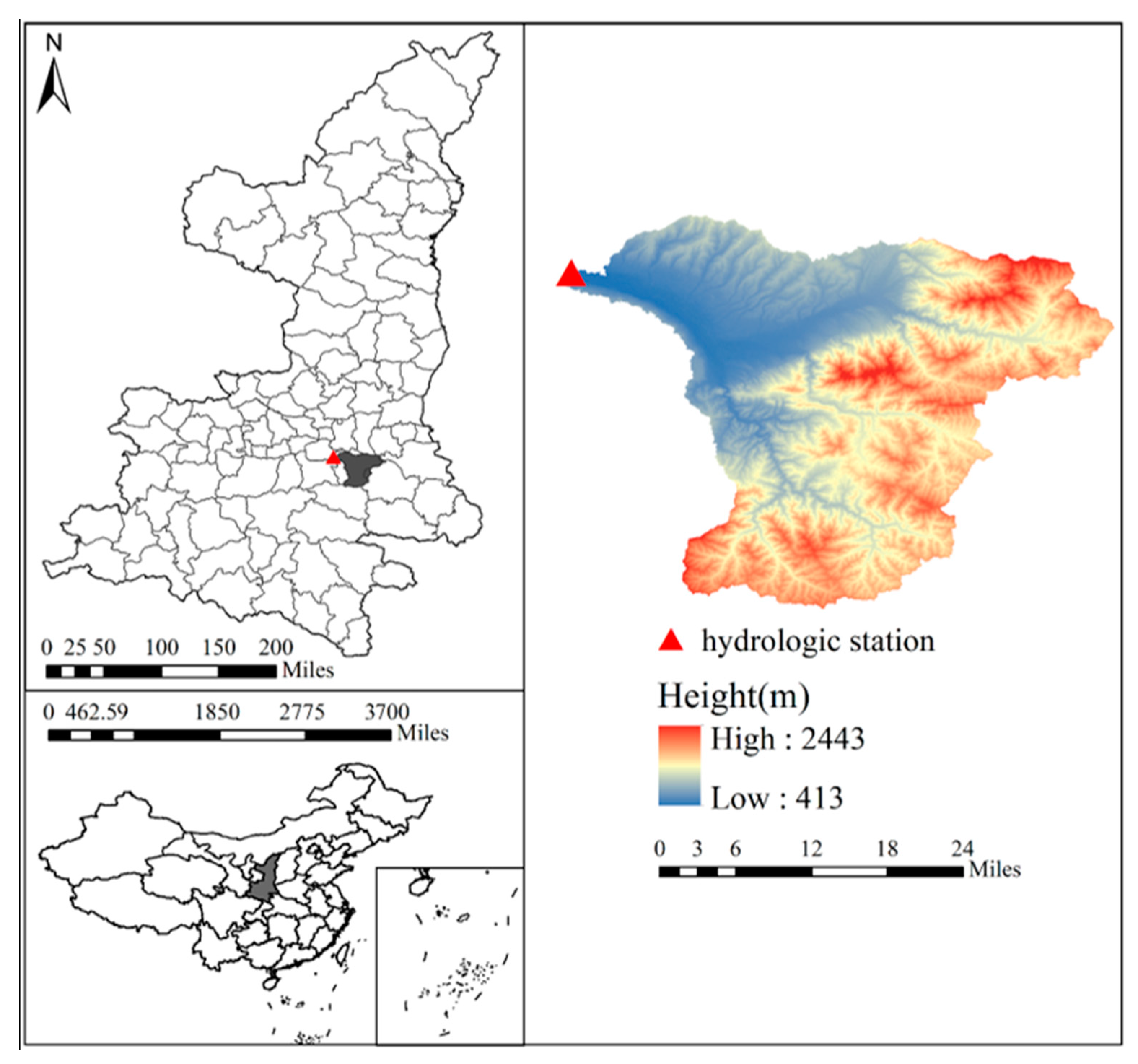
The study was conducted in the Bahe basin of China, which is in the northern part of the Qinling Mountains. The Ma Du Wang (MDW) hydrologic station was selected, located downstream in the Bahe basin; the watershed station before the Bahe River flows into the Weihe River. There is no large reservoir in the catchment. The catchment area is about 1760 (see Figure 1), the average elevation is 1170 m, and the land use is dominated by agriculture and forest. The average annual precipitation in the Bahe region is about 720 mm, and nearly 60% of precipitation occurs between July and October. Precipitation is the primary source of runoff, and the summer runoff accounts for more than 40% of annual runoff. According to the Köppen–Geiger climate classification, the watershed controlled by the MDW station belongs to Dwa and Dwb classes: monsoon-influenced hot/warm summer, semi-arid continental climate.
2.2. Data
The meteorological data in this study come from the National Meteorological Information Centre (NMIC) and applies the same site station information as He et al. [18]. In addition, the spatial interpolation method for areal mean precipitation and ET calculation is by the Simple Kriging, which is also the same as He et al. [18]. The runoff data are at the daily time scale in this study, obtained from the Yellow River Conservancy Commission (YRCC).
3. Methods
For this comparative analysis, a conceptual hydrological model, Xin An Jiang (XAJ), is calibrated with different objective functions under varied climates. More detailed information is shown in the following.
3.1. Hydrological Model and Model Optimization
In this study, the XAJ model, a conceptual rainfall-runoff model at a daily time step, is selected. The XAJ model was developed for relatively humid regions in China by Zhao et al. [19,20], which has become a widely used model in runoff simulation, water resources assessment, and climate change assessments (e.g., [21]). In this study area, this model has been validated [22], and the model structure applied here is the same as Lin et al. [23]. For a detailed model description, please check there.
To optimize the hydrological model parameter set, an effective global optimization algorithm, the shuffled complex evolution (SCE-UA) algorithm was used in this study. This algorithm is mainly based on the concept of information-sharing and natural biological evolution [24,25]. It has been widely used in hydrological model calibration (e.g., [26,27]).
3.2. Calibration Objective Functions
Summarizing currently used objective functions, three different classes of objectives were evaluated; Table 1 gives more detailed information. About the criteria, both NSE and KGE are widely used in hydrology, while KGE is free of the influence of unhelpful interactions among components [28]. Therefore, KGE has been analyzed and recommended by many studies (e.g., [29,30,31]) and is applied here.
The calculation of KGE follows Equation (1):
With
As shown in Table 1, it includes the single objectives, multi objectives, and split objectives. The single objective class, which includes OBJ1 and OBJ2, applies two different transformation approaches to the discharge in the KGE calculation. These transformations are considered to emphasize the low flow goodness of fit: one is the logarithmic transformed discharge [5,32,33] and another is the inverse transformed discharge [34]. For the multi objective class, which is from OBJ3 and OBJ6, follows the format from Garcia et al. [3], who combined the normal KGE with the inverse transformation-based KGE in the objective by the same weights for both the time-based and FDC-based series. Additionally, this study includes the logarithm transformation-based partners to explore the influence from the transformation selection. The last class considers the recommendation from Fowler et al. [35], who proposed the split KGE as the objective function and found it could significantly improve the model performance. To validate the improvement of this strategy, this split KGE is set as OBJ7. OBJ8 is proposed in this study, which applies this strategy to the suggested objective function (OBJ4) by Garcia et al. [3]. Regarding the above description, some connections or similarities exist between the evaluated objective functions, which is helpful to explore the characteristics by pair comparison.

Table 1.
The information of evaluated objective functions in this study.
| Classes | Criteria | Name | Description | Reference |
|---|---|---|---|---|
| Single objective | KGE(log(Q)) | OBJ1 | KGE calculated on logarithmic transformed discharges | Oudin et al. [33] |
| KGE(1/Q) | OBJ2 | KGE calculated on inverse transformed discharges | Pushpalatha et al. [34] | |
| Muti objective | KGE(Q)+KGE(log(Q)) | OBJ3 | Sum of KGE calculated on discharges and logarithmic transformed discharges | Proposed in this study |
| KGE(Q)+KGE(1/Q) | OBJ4 | Sum of KGE calculated on discharges and inverse transformed discharges | Garcia et al. [3] | |
| KGE(Qsort)+KGE(log(Qsort)) | OBJ5 | Sum of KGE calculated on the FDC and logarithmic transformed of the FDC | Proposed in this study | |
| KGE(Qsort)+KGE(1/Qsort) | OBJ6 | Sum of KGE calculated on the FDC and logarithmic transformed of the FDC | Garcia et al. [3] | |
| Split objective | split KGE(Q) | OBJ7 | Averaged KGE calculated on discharges in each year | Fowler et al. [35] |
| split (KGE(Q)+KGE(1/Q)) | OBJ8 | Averaged sum of KGE calculated on discharges and inverse transformed discharges in each year | Proposed in this study |
3.3. Model Performance Assessment
Climatic Robustness Assessment
The Differential Split-Sample Test (DSST) is applied to test the objective functions, where two independent periods are in different conditions [36]. According to the statistical climate analysis, the climate will be drier in the future in this region [18]. Considering this, the model is calibrated with a relatively wet climate and validated in a dry climate.
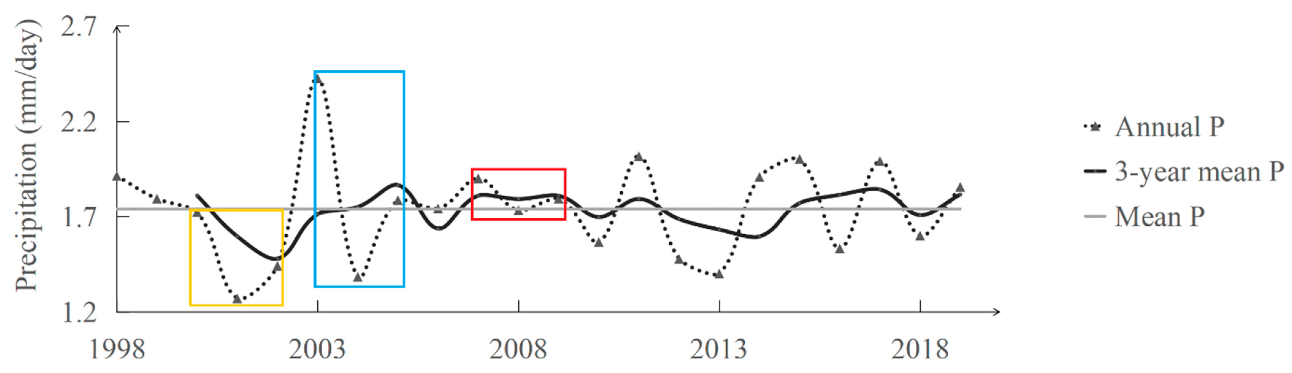
Figure 2 displays the precipitation information from 1998 to 2019 in the MDW station. It is easy to see that 2000–2002 is the only continuous period that every annual precipitation is lower than the average value; the annual precipitation is around 540 mm. To provide more valuable information for the application, as considered above, the period 2000–2002 is thus set as the validation period. Correspondingly, a relatively humid period is considered to be the calibration period. Through the plot, 2003–2005 shows the highest 3-year mean precipitation value (about 681 mm per year), making it as the calibration period. In order to increase the climatic robustness, the period 2007–2009 is also set as a calibration period, since its annual precipitation (about 661 mm per year) is higher than the average value in each year. In summary, two relatively humid periods (2003–2005 and 2007–2009) are applied for the calibration evaluation, and a relatively arid period (2000–2002) is used for the evaluation in this study.
3.4. Assessment Criteria
Paying more attention to the low flow simulation does not mean reducing the general performance. Therefore, the evaluation criteria used to compare the objective functions in this study are based on the general and the low flow simulation. Table 2 shows the applied assessment criteria correspondingly, including many low-flow indices used in hydrology [2,37]. For instance, the logarithmic transformed criteria have been widely used in studies, which shows overall goodness of fitting but emphasizes low flow [4,5,33]. Another class of low flow indices measure the low flow severity at different time steps, which is more concerned by water management agencies; for example, the mean annual 3-day minimum discharges. Moreover, the usage of FDC statistics increases, since it could provide valuable information in the frequency domain [11,38]. In this class, the LFD, Q95, and Q75 are applied in the study.
4. Results
4.1. Objective Functions Evaluation
4.1.1. Hydrograph Simulation
The time series of flow observation presents the temporal change in the water cycle in a basin, which is the base information for hydrological statistical analysis, such as the trend, the seasonality, etc. Therefore, assessing the performance of time series simulation is a vital evaluation aspect for objective functions.
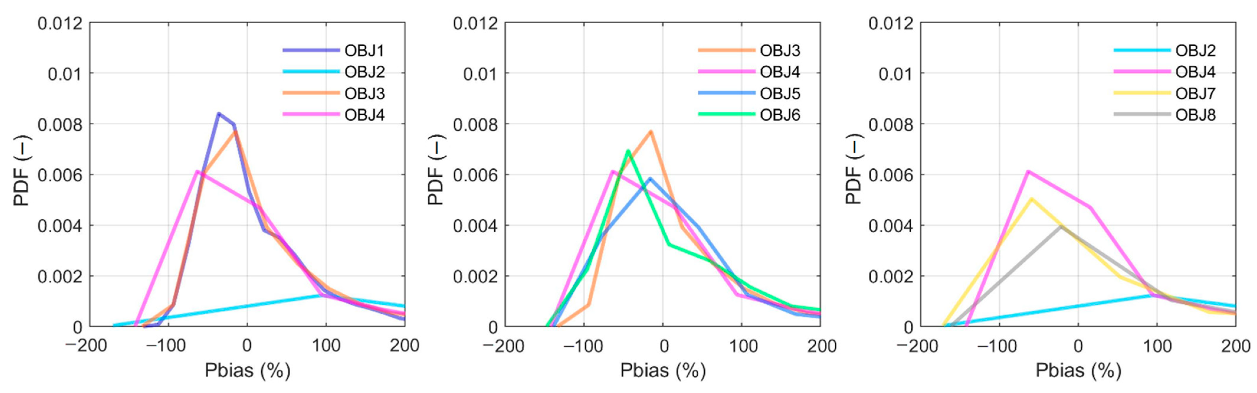
To compare the objective function influence on the time series simulation, Figure 3 displays the probability density function (PDF) of the percent bias (Pbias) information for the period of 2003–2005. The Pbias here divides the model residual by the observed flow value, which measures the general information for relative simulation errors. From the left subplot, the logarithmic transformed objective functions are better than the inverse transformed objective functions, regardless of whether the objective is single or multi. Taking the performance classification from Moriasi et al. [39], the days that achieved good simulation (|Pbias| < 15%) account for 45% and 44% during the calibration period by the OBJ1 and OBJ3, followed by OBJ4 with 40%, which is much higher than OBJ2. The result of acceptable performance (|Pbias| < 25%) also supports the above finding, where 61%, 60%, and 57% days are achieved by the OBJ1, OBJ3, and OBJ4, respectively. When comparing the single and multi-objectives, the above results indicate that the difference between single objectives (OBJ1 and OBJ2) is much more significant than the multi objectives (OBJ3 and OBJ4). Moving to the middle subplot, which shows the result from the multi objectives, the general probability of achieving smaller Pbias for objectives based on the time series seems higher than that based on the FDC. For instance, for OBJ5 and OBJ6, the days showing a good performance account for 45% and 26%, respectively, and the values change to 62% and 48% for acceptable performance. The right subplot shows the result from all three different kinds of objectives, and OBJ4 presents a better result than others, which means the split objective functions did not improve the simulation for the hydrological time series, while between two split objective functions, OBJ8 provides a slightly better simulation performance, which makes 2% and 1% days achieve a good and acceptable performance than OBJ7, correspondingly.
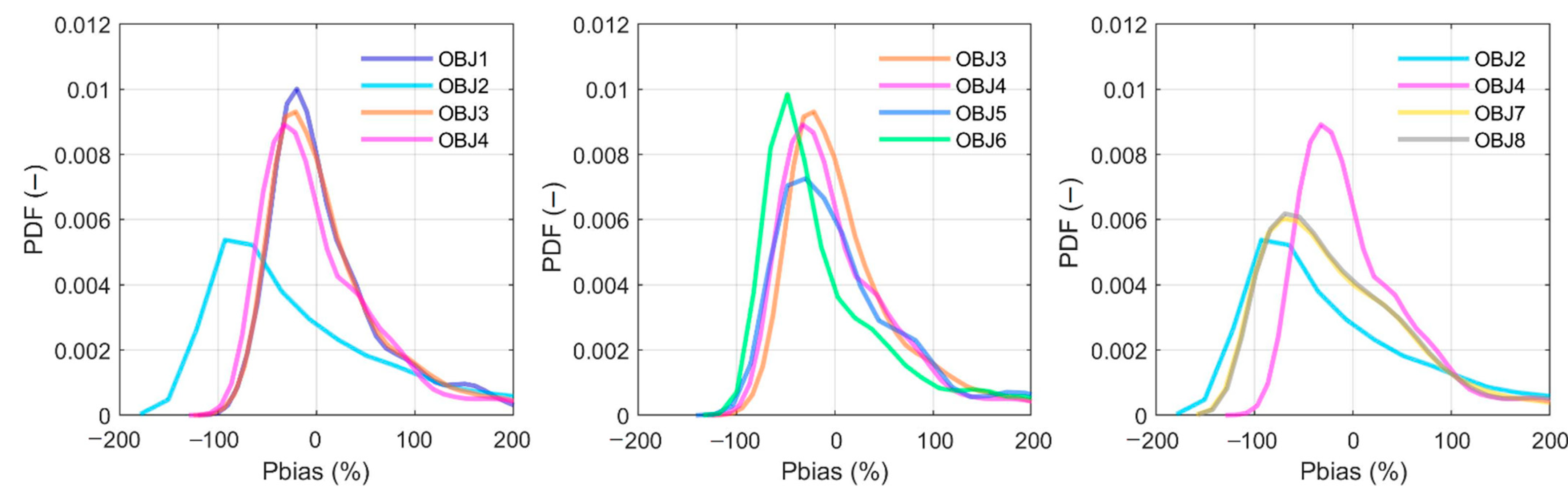
Figure 4 shows the same information as Figure 3, but for the calibration result during 2007–2009. Even though the general characteristics here are in line with Figure 3, minor differences exist. Although a clear distinction appears between single objectives (OBJ1 and OBJ2), the difference between multi objectives (see the middle subplot) is smaller than the period 2003–2005. Statistically, the days in good performance accounts for 45%, 44%, 36%, and 35%, and the values change to 64%, 58%, 53%, and 50% for acceptable performance for the OBJ3, OBJ4, OBJ5, and OBJ6, respectively.
The goodness of hydrograph fitting is also an essential measure for flow time series simulation, which has been evaluated frequently by KGE in recent years. Since this study focuses more on the low flow, the logarithmic transformed KGE results (KGElog) are also included. Table 3 presents the calculated values of KGE and KGElog during two calibration periods with all eight objective functions. In the table, the highest values for each period among objective functions are highlighted in bold, and ‘/’ is used when the value is lower than 0.
When looking at the KGE values, almost all objective functions show an acceptable performance in both calibration periods but with considerable differences. For example, during 2003–2005, the highest KGE is 0.92 from OBJ4, and the lowest value is 0.6 from OBJ2, while the difference between multi objectives is slight, which is 0.03 according to the result from 2003–2005. Comparing three different objectives classes, multi objectives show relatively higher KGE values, followed by split objectives and single ones. Focusing on the low flow simulation assessment by KGElog, three objectives produce values lower than 0, which means unacceptable. At the same time, all the multi objective functions provide good results, whose KGElog values are higher than 0.61. The highest KGElog value appears for OBJ1; this is mainly because the evaluation criterion is the same as the objective function and the KGElog values for OBJ3 are very close to OBJ1.
Considering the balance between general and low flow simulation through two periods, OBJ3 and OBJ4 yield relatively better results, followed by OBJ1. Taking the averaged KGE and KGElog values for the two periods as the example, the result is 0.821 and 0.797 for OBJ3 and OBJ4, respectively, followed by 0.773 for OBJ1. Among the multi objectives, regardless of whether it is time series-based or FDC-based, the logarithmic transformed objectives tend to yield higher averaged measurements than the inverse transformed objectives. The averaged KGE and KGElog value of the two periods for OBJ5 is 0.736, which is 0.685 for OBJ6.
4.1.2. Flow Duration Curves
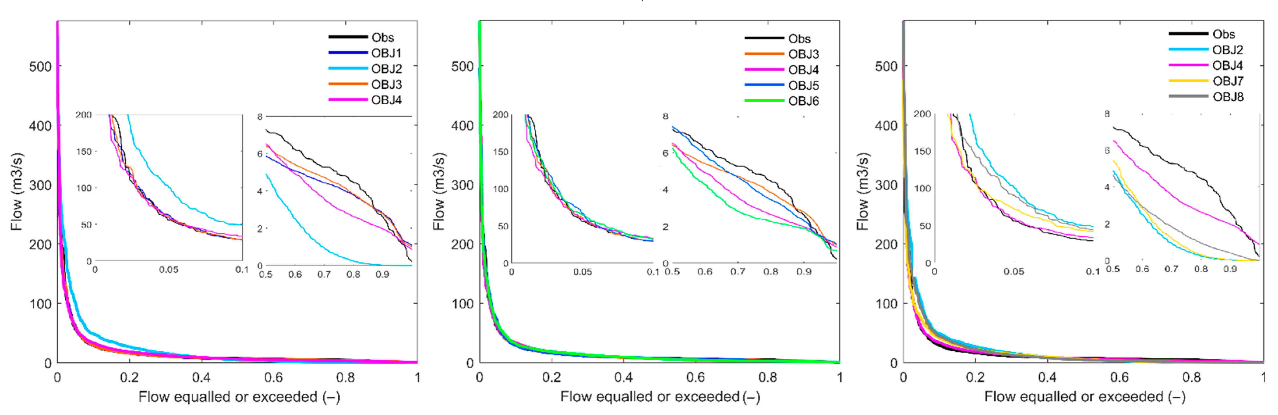
Unlike the time series evaluation, FDC statistics could provide valuable frequency domain information. Figure 5 presents the FDC assessment result overall for the eight objective functions during 2003–2005, and each subplot contains two zoomed subplots to more clearly present the results for high and relatively low flow simulations.
According to the left subplots, the simulated FDC from OBJ2 is far from all other curves, including the observation one. With the two zoomed subplots, OBJ2 presents substantial overestimation-to-observation for the highest 10% flow and heavy underestimation-to-observation for the lowest 50% flow. While the curves from OBJ1 and OBJ3 seem closer to the observation through two zoomed subplots, especially the low flow one. Compared with the left subplot, these multi objectives evaluated in the middle subplot produce more similar FDC simulations, especially for the high flows. While according to the zoomed low flow subplot, OBJ5 presents the closest FDC simulation to the observation, followed by OBJ3, and OBJ6 stays furthest. All simulated curves show a visible difference from the right subplot, more significant between each curve than from the left subplot. Among these objective functions, OBJ4 provides the closest simulation; the split objective functions work similarly to OBJ2.
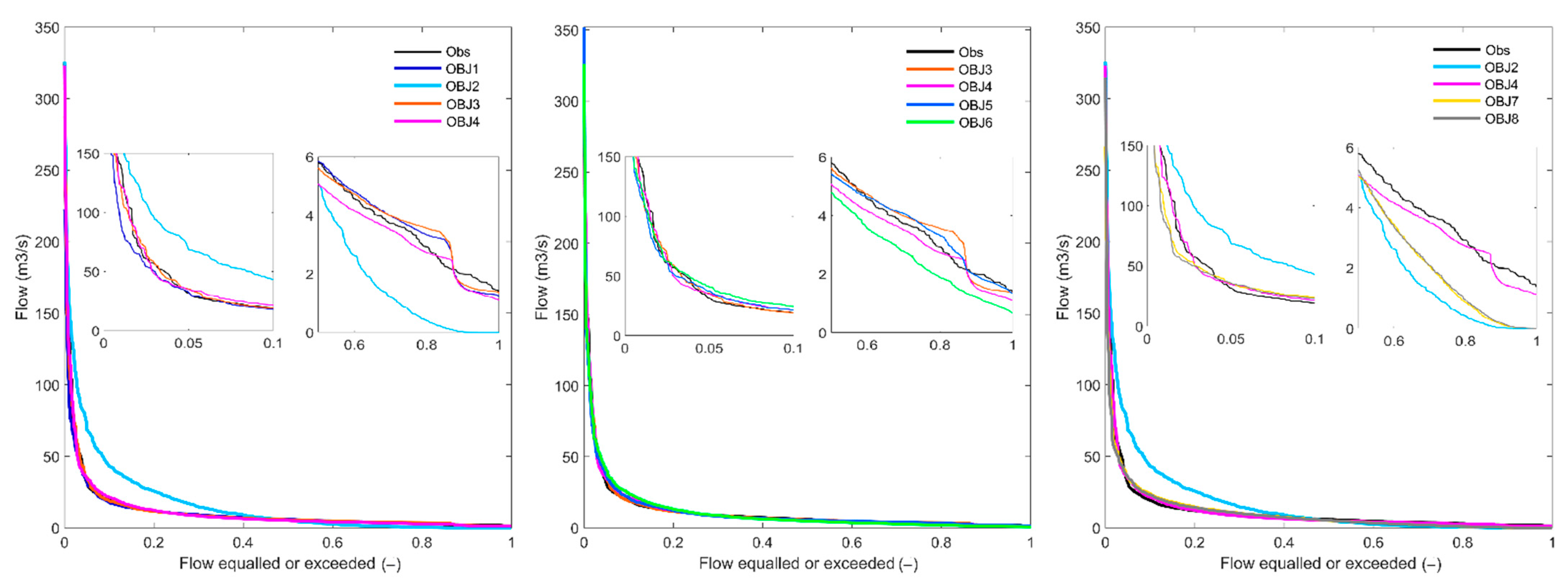
Figure 6 presents the results in the same way as in Figure 5 but is based on the calibration during 2007–2009. The general characteristics presented here totally agree with findings from Figure 5, regardless of the scale difference. For instance, the curve simulated by the OBJ2 stays visibly far from the observation curve, and OBJ5 and OBJ3 yield the closest simulation curve to the observation. However, the curves from the multi objectives keep close to each other.
4.1.3. Low Flow Indices
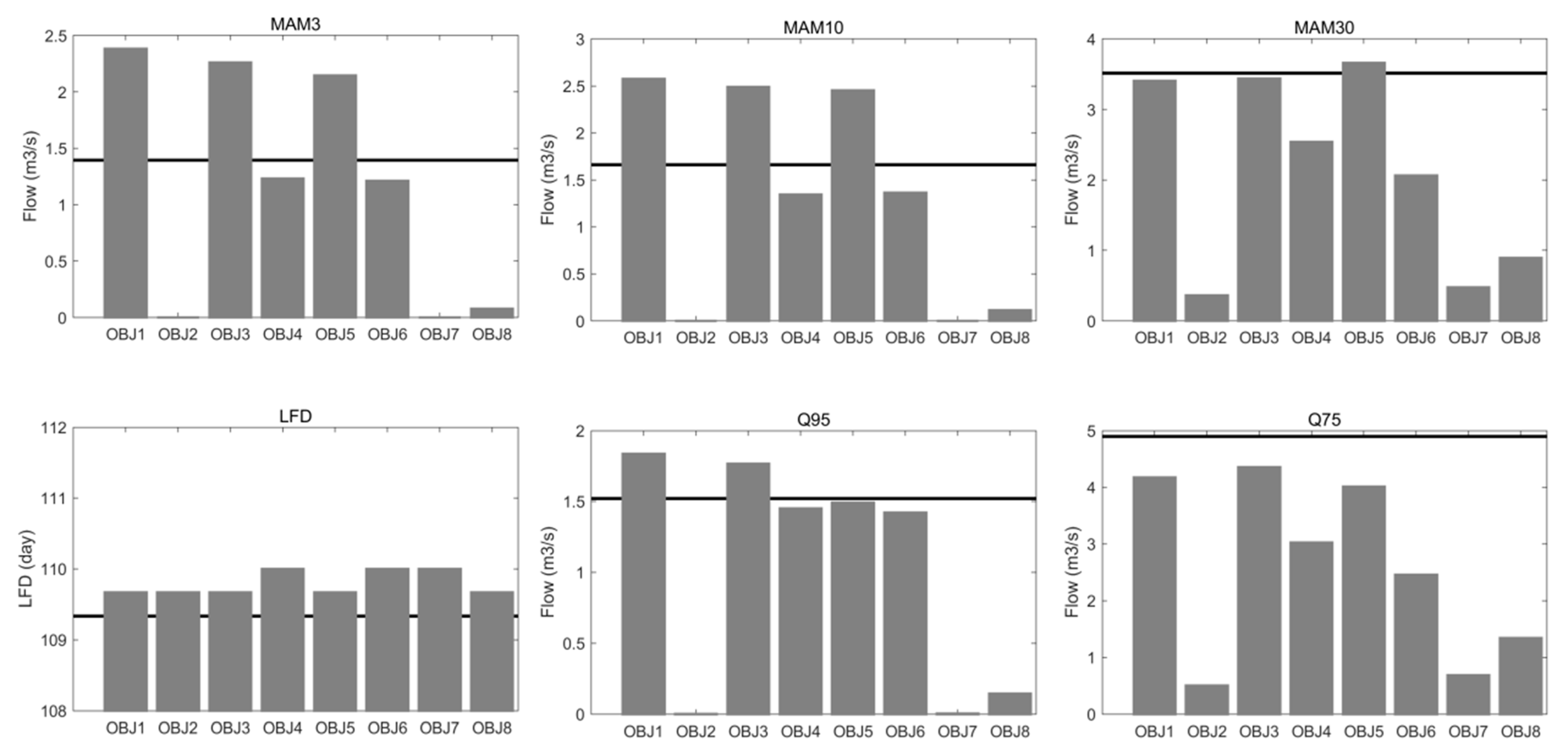
Since this study emphasizes low flow simulation, different low flow indices are thus applied in Figure 7, where the line shows the observed value and the bar presents the simulated value.
Through all subplots, the objective functions provide similarly good simulations to the observed LFD. Apart from the simulation of LFD, the objectives OBJ2, OBJ7, and OBJ8 vastly underestimate the other observed low flow indices, which are not comparable with other evaluated partners. Between the rest of the objectives, the inverse transformed objectives (OBJ4 and OBJ6) estimate the indices visibly lower than the logarithmic transformed ones (OBJ1, OBJ3, and OBJ5). For example, the average estimation for MAM3 is about 1.3 m3/s from the inverse transformed objectives, which is about 2.2 m3/s from the logarithmic transformed objectives.
Assessing the performance aspect, the inverse transformed objectives better estimate the indices sensitive to the extreme low flows (e.g., MAM3, MAM10, and Q95). According to the subplot for MAM10, the averaged estimation error is about 0.3 m3/s from the inverse transformed objectives, which climbs to 0.8 m3/s from the logarithmic partners. Conversely, the logarithmic transformed objectives provide a better estimation for the indices less sensitive to the extreme low flows (e.g., MAM30 and Q75). Observing the subplot for MAM30, the averaged estimation error is about 1.4 m3/s from the inverse transformed objectives, which is about 13 times for the logarithmic partners.
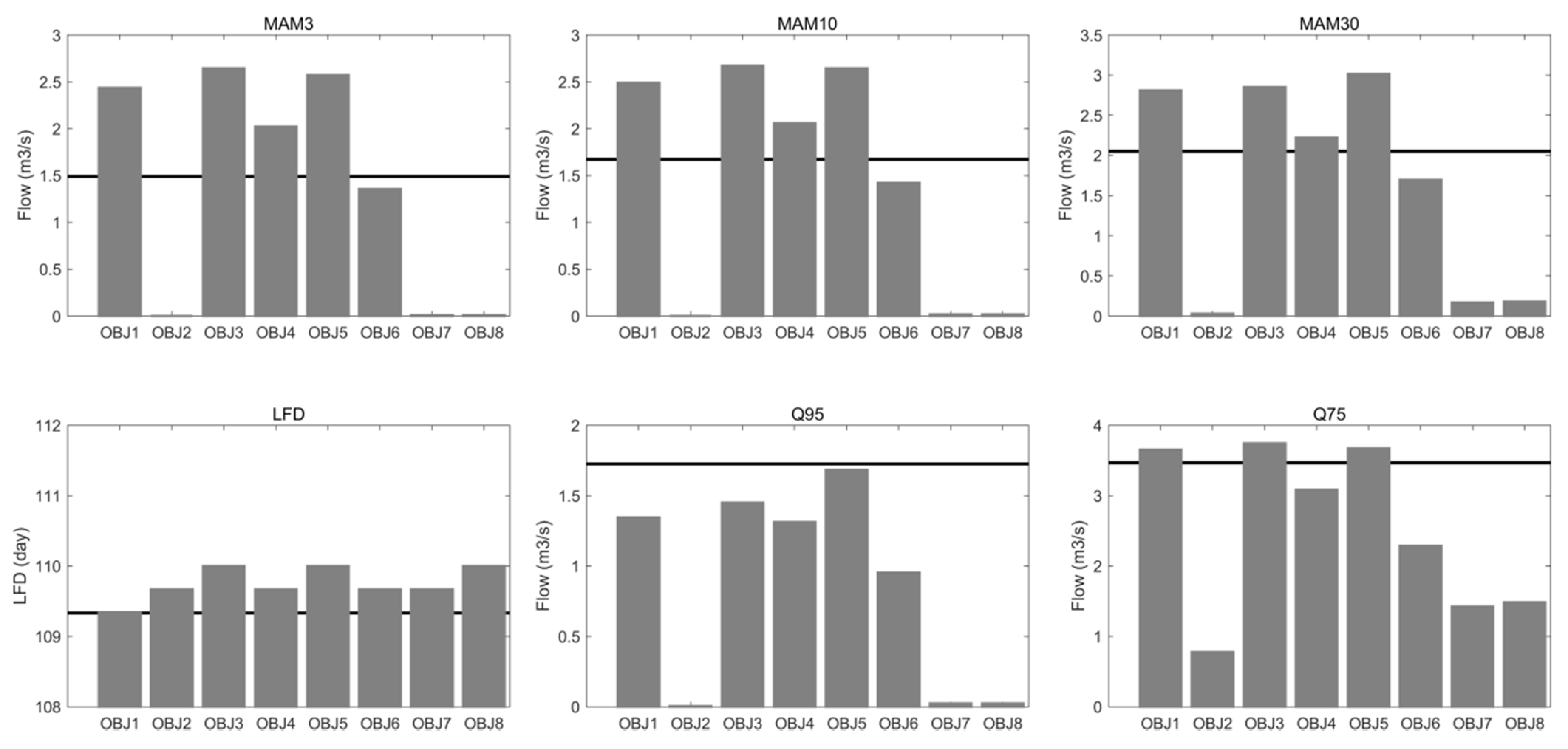
In Figure 8, the information is summarized similarly to Figure 7 but applies the data calibrated during 2007–2009. There are some of the same characteristics observed here as in Figure 7, such as the similar simulation from all objectives for LFD; unacceptable estimation by OBJ2, OBJ7, and OBJ8, and the higher estimation by logarithmic transformed objectives than the inverse transformed partners. However, the performance preference shows some differences here from Figure 7. First, OBJ6 produces a minor estimation error for the MAM3 and MAM10, while the OBJ5 yields almost the exact same estimation as the observed Q95. This result cannot support the finding in Figure 7 that the inverse transformed objectives produce a better estimation for the indices sensitive to the extreme low flows. Second, OBJ4 and OBJ5 provide the most similar estimation to the observed MAM30 and Q75, respectively. This result is not consistent with the finding that logarithmic transformed objectives provide a better estimation for the indices less sensitive to the extreme low flows.
4.2. Climatic Robustness Assessment
As mentioned above, the DSST method is applied to assess the climatic robustness of the objectives. To enhance the finding reliability and applicability, the climatic robustness evaluation validates the calibration result achieved in two different wet climate periods in a relatively dry climate.
4.2.1. Hydrograph Simulation
Figure 9 displays the observed and simulated hydrographs during the validation period, with the evaluated objectives, except for OBJ2, OBJ7, and OBJ8 due to the bad calibration.
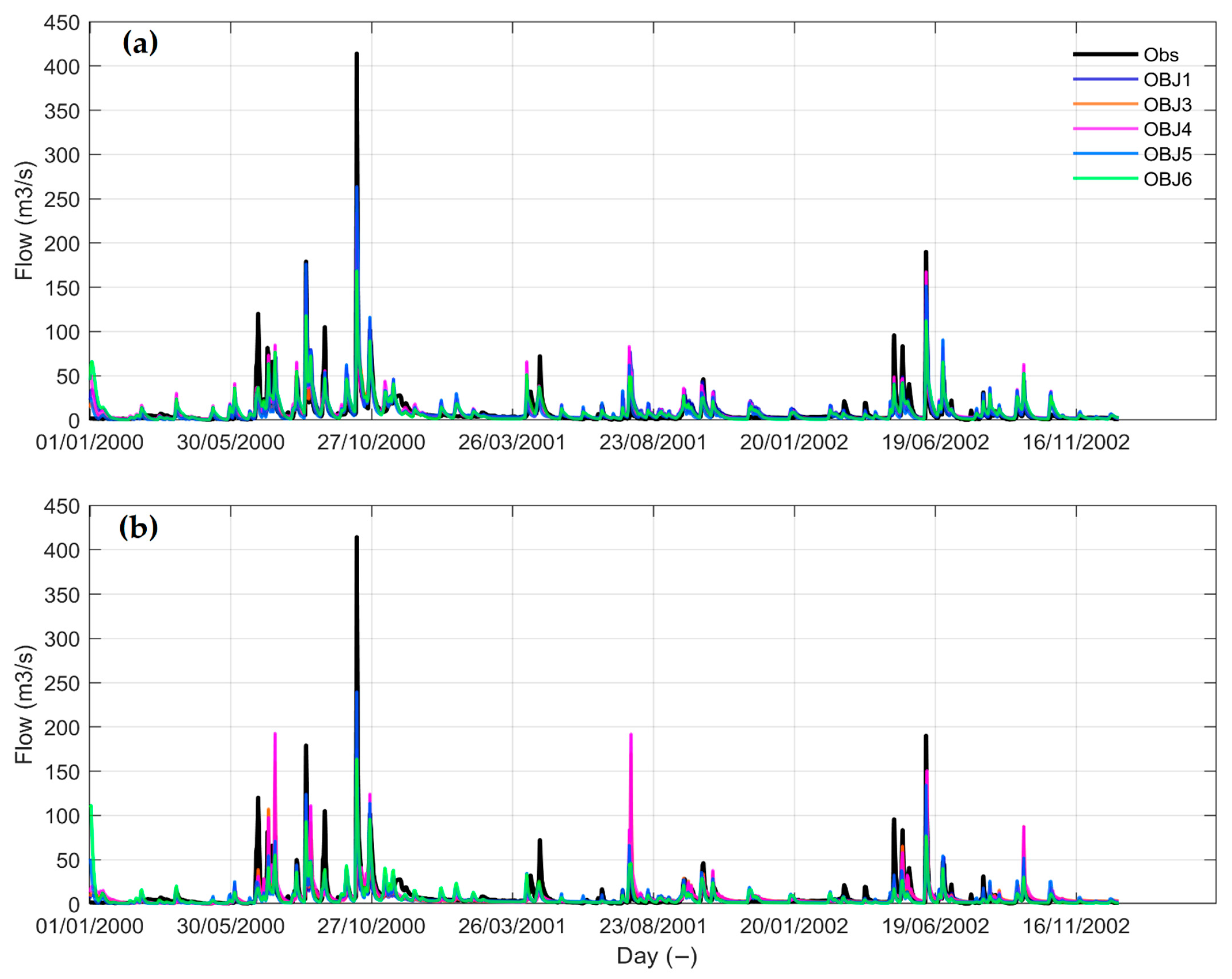
At first sight, even though the objectives are different, all simulations follow the observation temporal change pattern, and no apparent time jags appear in both subplots. From the upper subplot, OBJ5 shows a relatively better estimation for high flows, especially the peaks, followed by OBJ4, and other objective measures are comparable. In the lower subplot, OBJ4 tends to overestimate the high flows, except for the peak flow. The rest objectives present similar simulations for most time steps, except OBJ5 for some high flows. Evaluating the simulation performance between two periods, the estimated hydrographs based on the period 2003–2005 are generally closer to the observation than based on the period 2007–2009.
Due to the serious overlaps between hydrograph simulations, the information about the evaluated statistics (KGE and KGElog) is presented in Table 4 to provide more valuable information for hydrograph simulation evaluation.
Most of the objectives produce acceptable validation results based on both calibration periods. According to the values shown in the table, all the KGElog values are higher than 0.62, and most of the KGE values are higher than 0.58. As shown in bold text, all the highest values for both criteria appear in the multi objective group, and all the values are higher than 0.7, except the KGE value during 2007–2009. Between the evaluations based on two different calibration periods, all the KGE values based on the calibrated model during 2003–2005 are higher than 2007–2009, but the KGElog values are comparable. For example, when applying the OBJ1, the KGE value based on 2003–2005 is 0.19 higher than in 2007–2009, but the difference between the two KGElog values is only 0.02. Focusing on the low flow simulation through both validation results, if taking the averaged KGElog value as the measure, OBJ3 presents the best performance, with an averaged KGElog value of 0.69.
4.2.2. Flow Duration Curves
As mentioned above, FDC statistics could provide additional information to the time series simulation. Thus, the validation evaluation also includes the FDC assessment result. Figure 10 presents the corresponding result and the left and right penal subplot show the result based on the calibrated model during 2003–2005 and 2007–2009, respectively.
Overall, the simulated FDCs from all the objectives are comparable and not far from the observed FDC, consistent in both periods. Through the simulation for the highest 10% flow and the lowest 50% flow, the results of which are shown in the left and right zoomed subplots, respectively, the difference between objectives is large for the low flow simulations. Among the low flow simulation objectives, the FDC from OBJ5 seems closer to the observed curve in subplot (a), which changes to OBJ4 in subplot (b). In contrast, the simulated FDC from OBJ1 and OBJ6 in corresponding subplots (a) and (b) present a clear distance from the observation. In addition, the simulated FDCs tend to be higher than the observation in subplot (a), while they spread mixed on both sides of the observation in subplot (b).
4.2.3. Low Flow Indices
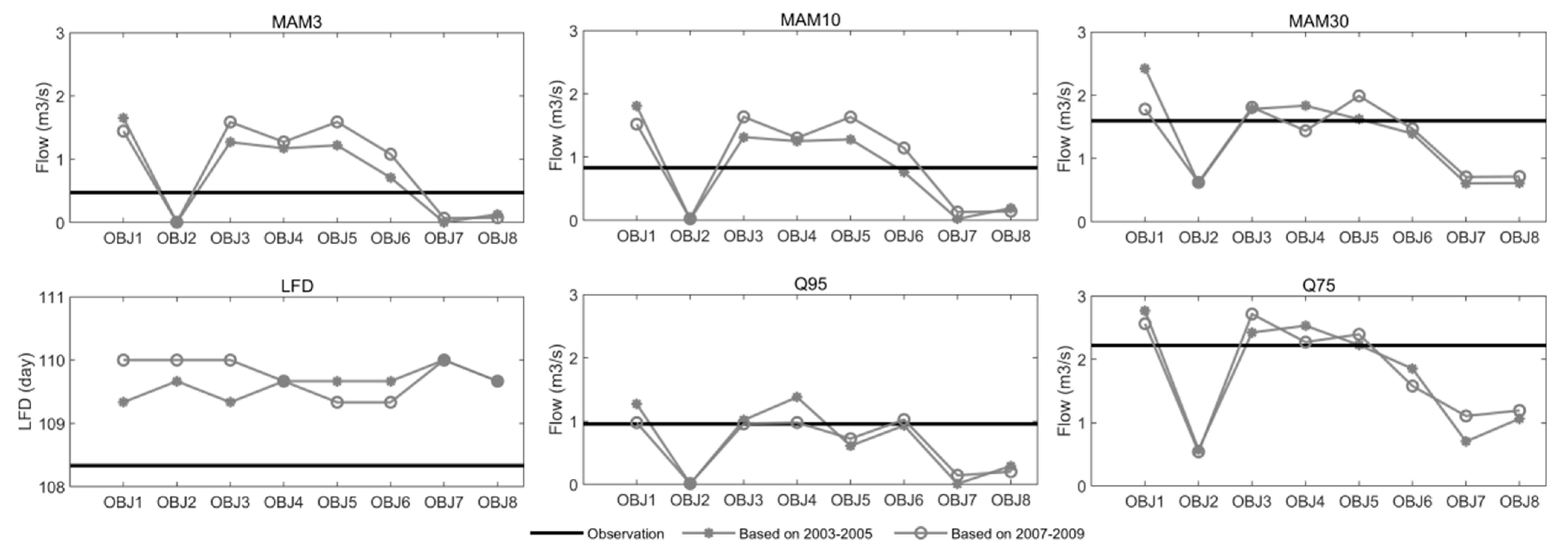
To further explore the objective influence on low flow simulation, Figure 11 displays the observed and simulated low flow indices during the validation period by applying the calibrated model based on different periods. Through the validated simulations, there is no apparent conflict result shown between the different calibration periods, therefore, the generated result over both periods is described below.
Consistent with the results shown in the calibration period. First, the OBJ2, OBJ7, and OBJ8 provide significantly different and worse estimations than other objectives for all evaluated low flow indices except LFD. Second, all the objectives based on both calibration periods appear similar to the simulation for LFD, which is about 1.2 days averagely longer than the observation. Third, all the left logarithmic transformed objectives (e.g., the OBJ1, OBJ3, and OBJ5) provide a relatively higher estimation than the inverse transformed partners (e.g., the OBJ4 and OBJ6), except for the Q95 simulation here.
Going through the simulation over upper subplots, the inverse transformed objectives appear closer to the observation, even though the observations between the three indices are clear. For instance, the estimated MAM30 from OBJ6 is only about 0.1 lower than the observation, while for the quartile indices, the simulations from the left objectives (e.g., the OBJ1, OBJ3, OBJ4, OBJ5, and OBJ6) are comparable, especially for Q95, whose range between those objectives is smaller than 0.5. Another interesting point is that for the logarithmic transformed objectives, the difference between the single objective and multi objectives is relatively smaller for extreme low flow indices. For example, the difference between the simulations from the three objectives is about 0.5 for the evaluation of MAM3, which increases to about 1 when assessing the MAM30.
5. Discussion
The hydrological models have been popularly applied in water research and application, while the objective functions that are suitable for calibrating the hydrological models for low flow simulation are unclear, especially in relatively arid regions. Therefore, a comprehensive evaluation of different kinds of objective functions in relatively dry areas will provide valuable information.
5.1. Objective Functions Evaluation
In the current study, eight objective functions were selected for model calibration, which belong to different classes. According to the above results, the logarithmic and inverse transformation formats shows a pronounced difference. This may be due to the high sensitiveness of the inverse transformation to extreme low values, as analyzed by Pushpalatha et al. [34]. In the model error term part, the inverse transformation gave more emphasis on low flows than the logarithm transformation. Another explanation may be that, at relatively arid regions, very low values appear frequently in observed flow, which enhances the weight on low flows. Second, our results suggest applying logarithm transformation rather than the inverse transformation in low flow studies, which differs from Pushpalatha et al. [34]. One possible reason may be that Pushpalatha et al. [34] applied NSE, and NSE is regarded to give more emphasis on high flow than KGE, which, thus, balances the low flow weight to some extent. Furthermore, despite the FDC simulation, the FDC-based multi objectives did not exhibit a better performance than the time series-based partners, which concurs with Garcia et al. [3]. As confirmed by the above results and analysis, OBJ3 is suggested for low flow simulation studies in relatively arid regions. It fails to agree with the finding by Garcia et al. [3], who recommended the OBJ4 as the sufficient calibration objective for low flow simulation based on the evaluation in a humid region. Therefore, the climate and geographic conditions may be the main factor for the disagreement between the two studies.
Comparing the single and the combined multi objective group from the performance over different aspects, the general performance applying combined multi objectives seems better. This result confirms the notion that the combined objectives could achieve an overall better benefit (e.g., [40]). The single objective is difficult to simulate all the hydrograph shape characteristics simultaneously (e.g., [41,42]). Furthermore, whether based on the time series or FDC, the performance difference between multi objectives appears smaller than between the single objectives. That means the simulation uncertainty is relatively smaller when applying the multi objectives, which is in line with the knowledge that multi objective calibration could mitigate the uncertainty issues (e.g., [43]). Regarding the performance from spit objectives, which is proposed and recommended by Fowler et al. [35], it seems the worst among all groups, especially for the simulation of low flow indices.
5.2. Climatic Robustness Assessment
To additionally explore their climatic robustness, the evaluation of their performance was based on two different calibration periods and a validation period, whose climatic conditions varied. Assessing from two calibration periods, the general observed characteristics of the results are consistent, although the performance values showed some differences. Furthermore, even though the average precipitation changed more than 20%, shown as the validation and calibration periods in this study, no noticeable changes were detected for the general observed characteristics. This is unlike the finding by Garcia et al. [3], who asserts that the robustness depends on the climate variability rather than the objective function. This difference of opinion may be related to the different magnitude. For example, the climate difference between the calibration and validation period in the current study is not big enough to explore the climatic influence. At the same time, a minor but interesting characteristic from the validation results is that the general performance difference between single and multi-objectives seems more significant based on the calibration with more considerable climate variability.
6. Conclusions
The accuracy of low flow simulation yield from the hydrological models presents an apparent effect on water management. Research on the suitableness evaluation of the calibration objectives is of importance. Aiming to enhance insight into the objective influence on low flow simulation in relatively arid regions, which prior to our research was very limited, this study evaluated eight different kinds of objective functions with varied climate conditions. The analysis was performed using the observation at Ma Du Wang station in the Bahe basin, China, located in a semi-arid and semi-humid continental climate region. The main conclusions from the study are summarized in the following points:
- -
- The influence of the included transformation formats in objective functions on low flow simulation is pronounced, and logarithmic transformation is recommended.
- -
- Among the three classes of objective functions, the combined multi-class is highly recommended, and the mean of KGE(Q) and KGE(log(Q)) remains a first choice. In contrast, the class of split objectives is regarded as the last choice as it demonstrated the worst performance.
- -
- Replacing the objective function from the time series based on the FDC could not improve the simulation performance.
Although this study evaluated the performance of different objectives under varied climates and achieved additional valuable knowledge, the current study has some limitations. First, including more hydrological models could help obtain more solid conclusions and deepen the understanding of model influence. In addition, assessing the performance under an increased number of varied climate conditions could broaden the knowledge about the climatic influence, which is essential for research concerning the changing climate.
Author Contributions
Conceptualization, X.Y. and B.Z.; methodology, X.Y.; software, X.Y.; validation, C.Y. and X.L.; formal analysis, X.L.; investigation, C.Y.; resources, J.L.; data curation, J.X.; writing—original draft preparation, X.Y.; writing—review and editing, X.Y. and C.Y.; visualization, X.L.; supervision, B.Z.; project administration, J.L.; funding acquisition, J.X. All authors have read and agreed to the published version of the manuscript.
Funding
This research was funded by the Education Department of Shaanxi Provincial Government (Project No. 21JT032) and Xi’an University of Technology (Project No. 256082016). The APC was funded by Xi’an University of Technology (Project No. 256082016).
Data Availability Statement
Data available upon request.
Conflicts of Interest
The authors declare that they have no known competing financial interests or personal relationships that could have influenced the work reported in this paper.
References
- Engeland, K.; Hisdal, H. A comparison of low flow estimates in ungauged catchments using regional regression and the HBV-model. Water Resour. Manag. 2009, 23, 2567–2586. [Google Scholar] [CrossRef]
- Lang Delus, C. Les étiages: Définitions hydrologique, statistique et seuils réglementaires. Cybergeo Eur. J. Geogr. 2011. [Google Scholar] [CrossRef]
- Garcia, F.; Folton, N.; Oudin, L. Which objective function to calibrate rainfall-runoff models for low-flow index simulations? Hydrol. Sci. J. 2017, 62, 1149–1166. [Google Scholar] [CrossRef]
- Zhang, R.; Liu, J.; Gao, H.; Mao, G. Can multi-objective calibration of streamflow guarantee better hydrological model accuracy? J. Hydroinform. 2018, 20, 687–698. [Google Scholar] [CrossRef]
- Kim, H.S.; Lee, S. Assessment of the adequacy of the regional relationships between catchment attributes and catchment response dynamics, calibrated by a multi-objective approach. Hydrol. Process. 2014, 28, 4023–4041. [Google Scholar] [CrossRef]
- Peel, M.C.; Blöschl, G. Hydrologic modelling in a changing world. Prog. Phys. Geogr. 2011, 35, 249–261. [Google Scholar] [CrossRef]
- Misgana, M.K. Model Performance Sensitivity to Objective Function during Automated Calibrations. J. Hydrol. Eng. 2012, 17, 756–767. [Google Scholar]
- Reed, P.M.; Hadka, D.; Herman, J.D.; Kasprzyk, J.R.; Kollat, J.B. Evolutionary multiobjective optimization in water resources: The past, present, and future. Adv. Water Resour. 2013, 51, 438–456. [Google Scholar] [CrossRef]
- Efstratiadis, A.; Koutsoyiannis, D. One decade of multi-objective calibration approaches in hydrological modelling: A review. Hydrol. Sci. J. J. Sci. Hydrol. 2010, 55, 58–78. [Google Scholar] [CrossRef]
- Pfannerstill, M.; Guse, B.; Fohrer, N. Smart low flow signature metrics for an improved overall performance evaluation of hydrological models. J. Hydrol. 2014, 510, 447–458. [Google Scholar] [CrossRef]
- Asadzadeh, M.; Leon, L.; McCrimmon, C.; Yang, W.; Liu, Y.; Wong, I.; Fong, P.; Bowen, G. Watershed derived nutrients for Lake Ontario inflows: Model calibration considering typical land operations in Southern Ontario. J. Gt. Lakes Res. 2015, 41, 1037–1051. [Google Scholar] [CrossRef]
- Coello, C.A.; Aguirre, A.H.; Zitzler, E. Evolutionary multi-objective optimization. Eur. J. Oper. Res. 2007, 181, 1617–1619. [Google Scholar] [CrossRef]
- Tian, F.; Hu, H.; Sun, Y.; Li, H.; Lu, H. Searching for an Optimized Single-objective Function Matching Multiple Objectives with Automatic Calibration of Hydrological Models. Chin. Geogr. Sci. 2019, 29, 934–948. [Google Scholar] [CrossRef]
- Chilkoti, V.; Bolisetti, T.; Balachandar, R. Multi-objective autocalibration of SWAT model for improved low flow performance for a small snowfed catchment. Hydrol. Sci. J. 2018, 63, 1482–1501. [Google Scholar] [CrossRef]
- Shafii, M.; De Smedt, F. Multi-objective calibration of a distributed hydrological model (WetSpa) using a genetic algorithm. Hydrol. Earth Syst. Sci. 2009, 13, 2137–2149. [Google Scholar] [CrossRef]
- Kim, H.S. Adequacy of a Multi-objective Regional Calibration Method Incorporating a Sequential Regionalisation. Water Resour. Manag. 2014, 28, 5507–5526. [Google Scholar] [CrossRef]
- Lombardi, L.; Toth, E.; Castellarin, A.; Montanari, A.; Bratha, A. Calibration of a rainfall-runoff model at regional scale by optimising river discharge statistics: Performance analysis for the average/low flow regime. Phys. Chem. Earth 2012, 42, 77–84. [Google Scholar] [CrossRef]
- He, Y.; Qiu, H.; Song, J.; Zhao, Y.; Zhang, L.; Hu, S.; Hu, Y. Quantitative contribution of climate change and human activities to runoff changes in the Bahe River watershed of the Qinling Mountains, China. Sustain. Cities Soc. 2019, 51, 101729. [Google Scholar] [CrossRef]
- Zhao, R.J.; Zhang, Y.L.; Fang, L.R.; Liu, X.R.; Zhang, Q.S. The Xinanjiang Model. In Hydrological Forecasting; IAHS Press: Wallingford, UK, 1980; pp. 351–356. [Google Scholar]
- Zhao, R.J. The Xinanjiang model applied in China. J. Hydrol. 1992, 135, 371–381. [Google Scholar]
- Yang, X.; Magnusson, J.; Huang, S.; Beldring, S.; Xu, C.Y. Dependence of regionalization methods on the complexity of hydrological models in multiple climatic regions. J. Hydrol. 2020, 582, 124357. [Google Scholar] [CrossRef]
- An, D.; Li, Z.J.; Kan, G.Y.; Li, Q.L. Comparison between the Application of Data-driven Model and Conceptual Model. Water Power 2013, 39, 9–12. [Google Scholar]
- Lin, K.; Liu, P.; He, Y.; Guo, S. Multi-site evaluation to reduce parameter uncertainty in a conceptual hydrological modeling within the GLUE framework. J. Hydroinform. 2014, 16, 60–73. [Google Scholar] [CrossRef]
- Duan, Q.; Sorooshian, S.; Gupta, V. Effective and efficient global optimization for conceptual rainfall-runoff models. Water Resour. Res. 1992, 28, 1015–1031. [Google Scholar] [CrossRef]
- Duan, Q.; Sorooshian, S.; Gupta, V.K. Optimal use of the SCE-UA global optimization method for calibrating watershed models. J. Hydrol. 1994, 158, 265–284. [Google Scholar] [CrossRef]
- Jeon, J.H.; Park, C.G.; Engel, B. Comparison of performance between genetic algorithm and SCE-UA for calibration of SCS-CN surface runoff simulation. Water 2014, 6, 3433–3456. [Google Scholar] [CrossRef]
- Zeng, Q.; Chen, H.; Xu, C.Y.; Jie, M.X.; Chen, J.; Guo, S.L.; Liu, J. The effect of rain gauge density and distribution on runoff simulation using a lumped hydrological modelling approach. J. Hydrol. 2018, 563, 106–122. [Google Scholar] [CrossRef]
- Gupta, H.V.; Kling, H.; Yilmaz, K.K.; Martinez, G.F. Decomposition of the mean squared error and NSE performance criteria: Implications for improving hydrological modelling. J. Hydrol. 2009, 377, 80–91. [Google Scholar] [CrossRef]
- Lobligeois, F.; Andréassian, V.; Perrin, C.; Tabary, P.; Loumagne, C. When does higher spatial resolution rainfall information improve streamflow simulation? An evaluation using 3620 flood events. Hydrol. Earth Syst. Sci. 2014, 18, 575–594. [Google Scholar] [CrossRef]
- Magand, C. Influence de la Représentation des Processus Nivaux sur L’hydrologie de la Durance et sa Réponse Auchangement Climatique. Ph.D. Thesis, Université Pierre et Marie Curie, Paris, France, 2014. [Google Scholar]
- Osuch, M.; Romanowicz, R.J.; Booij, M.J. The influence of parametric uncertainty on the relationships between HBV model parameters and climatic characteristics. Hydrol. Sci. J. 2015, 60, 1299–1316. [Google Scholar] [CrossRef]
- Legates, D.R.; McCabe, G.J. Evaluating the Use of “Goodness-of-Fit” Measures in Hydrologic and Hydroclimatic Model Validation. Water Resour. Res. 1999, 35, 233–241. [Google Scholar] [CrossRef]
- Oudin, L.; Andréassian, V.; Mathevet, T.; Perrin, C.; Michel, C. Dynamic averaging of rainfall-runoff model simulations from comple-mentary model parameterizations. Water Resour. Res. 2006, 42, W07410.1–W07410.10. [Google Scholar] [CrossRef]
- Pushpalatha, R.; Perrin, C.; Moine, N.L.; Andréassian, V. A review of efficiency criteria suitable for evaluating low-flow simulations. J. Hydrol. 2012, 420, 171–182. [Google Scholar] [CrossRef]
- Fowler, K.; Peel, M.; Western, A.; Zhang, L. Improved Rainfall-Runoff Calibration for Drying Climate: Choice of Objective Function. Water Resour. Res. 2018, 54, 3392–3408. [Google Scholar] [CrossRef]
- Klemeš, V. Operational testing of hydrological simulation models. Hydrol. Sci. J. 1986, 31, 13–24. [Google Scholar] [CrossRef]
- Laaha, G.; Blöschl, G. Seasonality indices for regionalizing low flows. Hydrol. Process. 2006, 20, 3851–3878. [Google Scholar] [CrossRef]
- Price, K.; Purucker, S.T.; Kraemer, S.R.; Babendreier, J.E. Tradeoffs among watershed model calibration targets for parameter estimation. Water Resour. Res. 2012, 48, W10542.1–W10542.16. [Google Scholar] [CrossRef]
- Moriasi, D.N.; Arnold, J.G.; Van Liew, M.W.; Bingner, R.L.; Harmer, R.D.; Veith, T.L. Model Evaluation guidelines for systematic quantification of accuracy in watershed simulations. Trans. ASABE 2007, 50, 885–900. [Google Scholar] [CrossRef]
- Matrosov, E.S.; Huskova, I.; Kasprzyk, J.R.; Harou, J.J.; Lambert, C.; Reed, P.M. Many-objective optimization and visual analytics reveal key trade-offs for London’s water supply. J. Hydrol. 2015, 531, 1040–1053. [Google Scholar] [CrossRef]
- Jie, M.X.; Chen, H.; Xu, C.Y.; Zeng, Q.; Tao, X. A comparative study of different objective functions to improve the flood forecasting accuracy. Hydrol. Res. 2016, 47, 718–735. [Google Scholar] [CrossRef]
- Kamali, B.; Mousavi, S.J.; Abbaspour, K.C. Automatic calibration of HEC-HMS using single-objective and multiobjective PSO algorithms. Hydrol. Process. 2013, 27, 4028–4042. [Google Scholar] [CrossRef]
- Her, Y.; Seong, C. Responses of hydrological model equifinality, uncertainty, and performance to multi-objective parameter calibration. J. Hydroinform. 2018, 20, 864–885. [Google Scholar] [CrossRef]
Figure 1.
The location and Digital Elevation Model (DEM) information of the study area.

Figure 2.
The precipitation (P) information in Ma Du Wang station, the blue and red window marks the calibration periods, and the yellow window marks the validation period.
Figure 2.
The precipitation (P) information in Ma Du Wang station, the blue and red window marks the calibration periods, and the yellow window marks the validation period.

Figure 3.
The probability density function (PDF) comparison for the objective functions evaluating by the percent bias (Pbias) during the calibration period 2003–2005.
Figure 3.
The probability density function (PDF) comparison for the objective functions evaluating by the percent bias (Pbias) during the calibration period 2003–2005.

Figure 4.
The probability density function (PDF) comparison for the objective functions evaluating by the percent bias (Pbias) during the calibration period 2007–2009.
Figure 4.
The probability density function (PDF) comparison for the objective functions evaluating by the percent bias (Pbias) during the calibration period 2007–2009.

Figure 5.
The result of the observed and simulated FDCs by all objective functions during the calibration period 2003–2005. The zoomed plots in each subplot show the result for the highest 10% flow (left) and the lowest 50% flow (right) simulations.
Figure 5.
The result of the observed and simulated FDCs by all objective functions during the calibration period 2003–2005. The zoomed plots in each subplot show the result for the highest 10% flow (left) and the lowest 50% flow (right) simulations.

Figure 6.
The result of the observed and simulated FDCs by all objective functions during the calibration period 2007–2009. The zoomed plots in each subplot show the result for the highest 10% flow (left) and the lowest 50% flow (right) simulations.
Figure 6.
The result of the observed and simulated FDCs by all objective functions during the calibration period 2007–2009. The zoomed plots in each subplot show the result for the highest 10% flow (left) and the lowest 50% flow (right) simulations.

Figure 7.
The observed (the line) and simulated (the bars) low flow indices by all objective functions during the calibration period 2003–2005.
Figure 7.
The observed (the line) and simulated (the bars) low flow indices by all objective functions during the calibration period 2003–2005.

Figure 8.
The observed (the line) and simulated (the bars) low flow indices by all objective functions during the calibration period 2007–2009.
Figure 8.
The observed (the line) and simulated (the bars) low flow indices by all objective functions during the calibration period 2007–2009.

Figure 9.
The hydrograph plot during the validation period based on the calibration period (a) 2003–2005 (b) 2007–2009.
Figure 9.
The hydrograph plot during the validation period based on the calibration period (a) 2003–2005 (b) 2007–2009.

Figure 10.
The observed and simulated FDCs for the validation period based on the calibration in (a) 2003–2005 (b) 2007–2009. The zoomed plots in each subplot show the result for the highest 10% flow (left) and the lowest 50% flow (right) simulations.
Figure 10.
The observed and simulated FDCs for the validation period based on the calibration in (a) 2003–2005 (b) 2007–2009. The zoomed plots in each subplot show the result for the highest 10% flow (left) and the lowest 50% flow (right) simulations.

Figure 11.
The observed and simulated low flow indices by all objective functions during the validation period.
Figure 11.
The observed and simulated low flow indices by all objective functions during the validation period.

Table 2.
The applied criteria of performance evaluation in this study.
| Criteria | Description |
|---|---|
| KGE | Kling-Gupta Efficiency (see Equation (1)) |
| KGElog | KGE calculated on logarithmic transformed flow |
| MAM3 | Mean Annual Minimum 3-day mean flow at 3-year return period |
| MAM10 | Mean Annual Minimum 10-day mean flow at 3-year return period |
| MAM30 | Mean Annual Minimum 30-day mean flow at 3-year return period |
| LFD | The duration of low flow smaller than 30% of the time |
| Q95 | Flow exceeded 95% of the time |
| Q75 | Flow exceeded 75% of the time |
Table 3.
The calibrated KGE and KGElog values during two calibration periods.
| Evaluation Criteria | KGE | KGElog | ||
|---|---|---|---|---|
| Calibration Period | 2003–2005 | 2007–2009 | 2003–2005 | 2007–2009 |
| OBJ1 | 0.85 | 0.63 | 0.78 | 0.84 |
| OBJ2 | 0.60 | 0.25 | / | / |
| OBJ3 | 0.90 | 0.78 | 0.77 | 0.83 |
| OBJ4 | 0.92 | 0.78 | 0.70 | 0.79 |
| OBJ5 | 0.89 | 0.62 | 0.74 | 0.69 |
| OBJ6 | 0.90 | 0.55 | 0.68 | 0.61 |
| OBJ7 | 0.85 | 0.68 | / | / |
| OBJ8 | 0.74 | 0.69 | / | / |
Note: ‘/’ is used when the value is lower than 0.
Table 4.
The validated KGE and KGElog values yield by different calibrated models.
| Calibration Period | 2003–2005 | 2007–2009 | ||
|---|---|---|---|---|
| Evaluation Criteria | KGE | KGElog | KGE | KGElog |
| OBJ1 | 0.61 | 0.67 | 0.42 | 0.69 |
| OBJ3 | 0.68 | 0.70 | 0.58 | 0.68 |
| OBJ4 | 0.68 | 0.62 | 0.61 | 0.71 |
| OBJ5 | 0.79 | 0.67 | 0.58 | 0.63 |
| OBJ6 | 0.61 | 0.64 | 0.49 | 0.67 |
Publisher’s Note: MDPI stays neutral with regard to jurisdictional claims in published maps and institutional affiliations. |
© 2022 by the authors. Licensee MDPI, Basel, Switzerland. This article is an open access article distributed under the terms and conditions of the Creative Commons Attribution (CC BY) license (https://creativecommons.org/licenses/by/4.0/).
Share and Cite
MDPI and ACS Style
Yang, X.; Yu, C.; Li, X.; Luo, J.; Xie, J.; Zhou, B. Comparison of the Calibrated Objective Functions for Low Flow Simulation in a Semi-Arid Catchment. Water 2022, 14, 2591. https://doi.org/10.3390/w14172591
AMA Style
Yang X, Yu C, Li X, Luo J, Xie J, Zhou B. Comparison of the Calibrated Objective Functions for Low Flow Simulation in a Semi-Arid Catchment. Water. 2022; 14(17):2591. https://doi.org/10.3390/w14172591
Chicago/Turabian StyleYang, Xue, Chengxi Yu, Xiaoli Li, Jungang Luo, Jiancang Xie, and Bin Zhou. 2022. "Comparison of the Calibrated Objective Functions for Low Flow Simulation in a Semi-Arid Catchment" Water 14, no. 17: 2591. https://doi.org/10.3390/w14172591
Note that from the first issue of 2016, this journal uses article numbers instead of page numbers. See further details here.