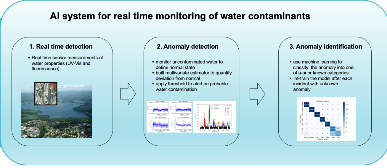
1. Introduction
Water-related issues will grow more pressing in the coming years. Water quality and availability will face substantial challenges as ever-growing populations in expanding global economies deal with the effects of climate change. The quality of water is critical for human development and ecosystem services [
1]. This goes beyond conventional pollutants and metrics of water-quality such as nitrogen, phosphorous, pH, dissolved oxygen, conductivity, turbidity, and dissolved organic carbon [
2]. The United States Environmental Protection Agency (USEPA) hosts a database of over 900 thousand chemicals in its effort to minimize risks to public health and the environment as a result of any unintended consequences resulting from the use of chemicals [
3]. To guarantee proper resource management, low-cost systems for monitoring water quality and detecting anomalies arising from a vast array of potential chemical contaminants are required.
A key aspect of such systems will be their capacity to provide warnings for changes in quality that may represent a risk to human health and the environment, as well as for the quality of products and services that use water. The importance of timeliness in such warnings means that a comprehensive investigation that takes hours or days is insufficient. Thus, online and real-time data are required for measurable impact in this regard.
To detect organic chemical pollutants in water, optical sensors based on absorption spectroscopy in the ultraviolet and visible range of the light spectrum (UV-spec) can be used. Furthermore, a complete (200–360 nm) spectrum assessment can reveal the types of substances present [
4]. The use of fluorescence spectroscopy to detect and identify pollutants is also common [
5]. The simultaneous monitoring of both absorbance and fluorescence changes can be an effective method for analyzing water quality online and in real time. Combined measurements of both absorbance and fluorescence can be used to build statistical models of normal and contaminated water.
The first aim of this study was to build an Artificial Intelligence (AI) tool, which can warn of a measurable change in water quality in real time based on the statistical models. The detection of such an occurrence could lead to a variety of measures, including automatic sample collection for further analysis. The second aim was to investigate the efficiency of such a system at classifying the cause of measurable changes in water quality (that is, not only detecting an anomaly but also indicating the nature of the anomaly). For this, the power of combining full-spectrum UV-spec and multi-channel fluorescence data was investigated.
2. Materials and Methods
2.1. Materials
Municipal drinking water from Oslo (Norway) was used for all benchmarking experiments in this study. The supply was obtained from Maridalsvannet lake, which has a surface area of 3.8 square kilometers. Normal variations in physiochemical parameters of the supply include pH 7.37–7.55, conductivity 8.7–10.0 mS/m, and turbidity 0.05–0.12 FTU [
6].
The focus of the AI development was to establish a means of categorizing “normality” (i.e., normal water quality) within a given aqueous environment such that any deviation from that normality can be detected. To push the water outside the bounds of this defined normality, some chemicals were selected as model contaminants and added to the respective water samples. No list could ever adequately cover the breadth of potential chemical contaminants in water; thus, the choice of substances for this study is not expected to be exhaustive. The list includes a small number of substances that represent a set of potential use cases only.
6-chloronicotinic acid (6CNA, CAS 5326-23-8) is a degradation product of neonicotinoid insecticides imidacloprid and acetamiprid. 2-mercaptobenzothiazole (MBT, CAS 149-30-4) is a probable carcinogen used in the vulcanization of rubber, which may come into contact with potable water and potentially from vehicle tire-wear-related pollution [
7]. Creatinine (CTN, CAS 60-27-5) is excreted in human urine in conjunction with protein metabolism. It provides an excellent biomarker for urinary contamination [
8]. Tryptophan (TPN, CAS 54-12-6) is an amino acid that is present in many foods that are rich in proteins. Some organic matter also fluoresces at the same wavelengths as tryptophan [
9]. The presence of organic matter in water, such as sewage and farm wastes, is linked to ‘tryptophan-like’ fluorescence [
10]. Spiking solutions of each of 6CNA, MBT, CTN, and TPN at 0.1 mg/mL were prepared in 20% methanol in water. Pyrene (PYR, CAS 129-00-0) and Benzo(a)pyrene (BAP, CAS 50-32-8) are polycyclic aromatic hydrocarbons (PAH) produced in a wide range of combustion reactions, including vehicle engines [
11]. Spiking solutions of PYR and BAP at 0.1 mg/mL were prepared in acetonitrile. The six chemicals, 6CNA, MBT, CTN, TPN, PYR, and BAP, were supplied by Merck Life Science AS (Oslo, Norway).
2.2. Experimental Setup
The setup comprised three field deployable sensors, a full scan UV-spec spectrometer, and two fluorometers. The UV-spec spectrometer (TriOS, OPUS) had a resolution of 0.8 nm/pixel and measured spectrum over the range between 200 and 360 nm [
12]. One of the fluorometers (TriOS, enviroFlu) was designed to detect polycyclic aromatic hydrocarbons (PAH) in water with excitation/emission wavelengths of 254/360 nm [
13] The other fluorometer (TriOS, matrixFlu VIS) was a general-purpose unit [
14], and we found excitation/emission wavelengths of 375/460 nm relevant for these studies.
All sensors were submerged in a water container with an inlet connected to the tap water and an outlet with a plug. Such a setup allowed for continuous flow-through at a replenishment rate of 2–4 cycles per hour when both the tap and the plug were opened. Three small aquarium pumps were installed to improve circulation and to prevent bubbles from accumulating on the sensor lenses. The entire setup was covered with a thick black plastic cover to avoid surrounding light interferences.
2.3. Data Acquisition and Pre-Processing
2.3.1. Data Acquisition
To establish systematic variabilities, drinking water was measured with continuous flow-through over a period of a few days (4–14). UV-spec data were recorded every minute, and fluorometer measurements were triggered every 30 s. We collected three datasets of 26,318, 7798, and 6453 points, which constituted baseline absorbance, baseline fluorescence 254/360, and baseline fluorescence 375/460, respectively, for statistical analysis. We define Absorbance variability ΔAbso as the difference between absorbance measured at a given point in time and the mean absorbance over the entire data-collection period. Similarly, fluorescence variability ΔFl is the difference between the fluorescence measured at a given point in time and the mean fluorescence over the entire data collection period.
The sensitivity for detection of anomalies in water was tested by performing spiking experiments. One experiment was performed for each of the six contaminants. Each experiment started with fresh tap water. Each contaminant was spiked numerous times and the acquisition was repeated at many spiking concentrations in order to establish an overall sensitivity for the system relative to varying contaminant loads. The tested concentration ranges were 15–1555 µg/L for 6CNA, 4–108 µg/L for MBT, 55–333 µg/L for CTN, 3–71 µg/L for TPN, 0.18–22 µg/L for PYR, and 1–26 µg/L for BAP. To ensure a stable concentration of each contaminant event, water replenishment was stopped for the duration of each spike. Mixing was, however, maintained via continuous operations of the aquarium pumps throughout the experiment. Data were collected for approximately 10 min before subsequent spikes.
2.3.2. Data Pre-Processing and Creation of Synthetic Time Series
Baseline UV-spec data of uncontaminated drinking water were corrected for biofouling effect, as described in
Appendix A. It should be stressed that during field operation, this artifact can be avoided by extra cleaning options installed on the lens [
15].
Signals for each concentration of added contaminant were averaged over the time interval being measured, with the exception of the first two minutes after spiking to make sure that the chemicals were properly mixed. Since absorbance is additive, signal absorbance (SAbso) was calculated for each concentration by subtracting average baseline absorbance prior to spiking. Thus, SAbso is a measure of how much light is absorbed by the added chemical. Under normal conditions without quenching fluorescence, it is proportional to the number of fluorophores added and, therefore, proportional to the concentration. Similarly, relative to SAbso, signal fluorescence (SFl) was calculated by subtracting baseline fluorescence prior to spiking. Fluorescent values for lower concentrations of BAP and TPN were obtained using linear extrapolation.
The synthetic time series (STS) of baseline with the anomaly of a desired type occurring at a chosen period can be generated by adding SAbso and (SFl) to match the baseline due to the additive nature of both absorbance and fluorescence. Because electronic noise is much lower than the natural variability of baseline levels, the statistical uncertainties of SAbso and (SFl) were neglected.
2.3.3. Feature Extraction
At each point in time, 200 measurements of absorbance (i.e., one per wavelength) were generated during data generation. To remove multi-collinearity in the data and to facilitate the analysis process, we applied principal component analysis (PCA) to reduce dimensionality. For building anomaly detection and identification systems, the leading five PCA components (accounting for 99% of data variance) of UV-spec and the two fluorescence channels were used. The system will depend on the 7 extracted variables in total for the anomaly detection process. The scikit-learn implementation of PCA was used [
16].
2.4. Anomaly Detection
The anomaly detection system is designed to detect measurements that vary significantly from the measured baseline and can indicate poor water quality or the presence of contaminants. Our baseline model is a multivariate Gaussian distribution with seven variables taht are the extracted features described in
Section 2.3.3. By construction, principal components (PCs) are uncorrelated. Baseline fluorescence is noise and, therefore, uncorrelated with PCs. Given no correlation between features, the covariance matrix simplifies into the diagonal terms, and the likelihood of the data given the baseline model (
L(
μ,σ;x)) can be written as follows [
17]:
where
μi and
σi are the mean and the standard deviation for the
ith dimension, respectively.
In this case, the maximum log-likelihood ratio simplifies into the following.
Λ(μ,σ;x) follows a χ2 distribution with n degrees of freedom and, therefore, can be directly linked to the probability of the measurement at a given timestamp, and it is compliant with the baseline.
2.5. Anomaly Identification
Anomaly identification is a classical multiclass categorization problem. There are several ML techniques well-suited for addressing this problem. For the sake of simplicity, we assumed that there might only be one chemical contaminant present in any given event; therefore, there is no interaction between target categories. We used the scikit-learn [
16] implementation of multinomial logistic regression (LR) [
18] to determine the category of chemicals that the anomaly belongs. Target categories need to be known beforehand. In our studies, we used the six chemicals listed in
Section 2.1 to train and test the model.
3. Results
3.1. Baseline and Signals
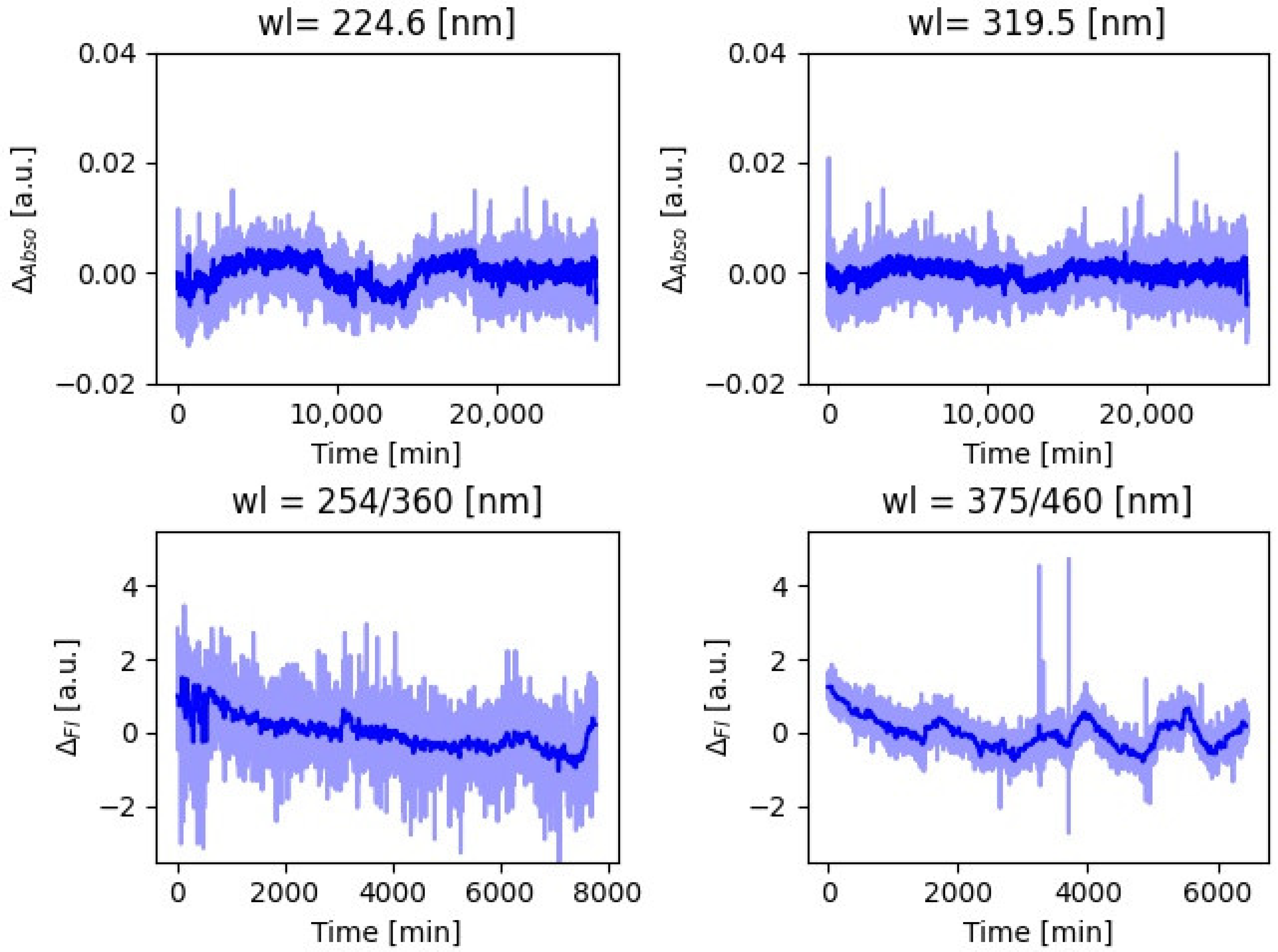
Figure 1 shows the baseline variability, caused by water quality, for the two selected absorbance and the two fluorescence wavelengths. Absorbance data were corrected for biofouling effect as explained in
Appendix A. To reduce statistical fluctuations, variability was averaged over 10 min intervals. For absorbance, one standard deviation (σ) equals 0.0021 for the 224.6 nm and 0.0012 for 319.5 nm wavelengths, respectively. For fluorescence, σ = 0.45 for 254/360 nm and σ = 0.40 for 375/460 nm wavelength, respectively.
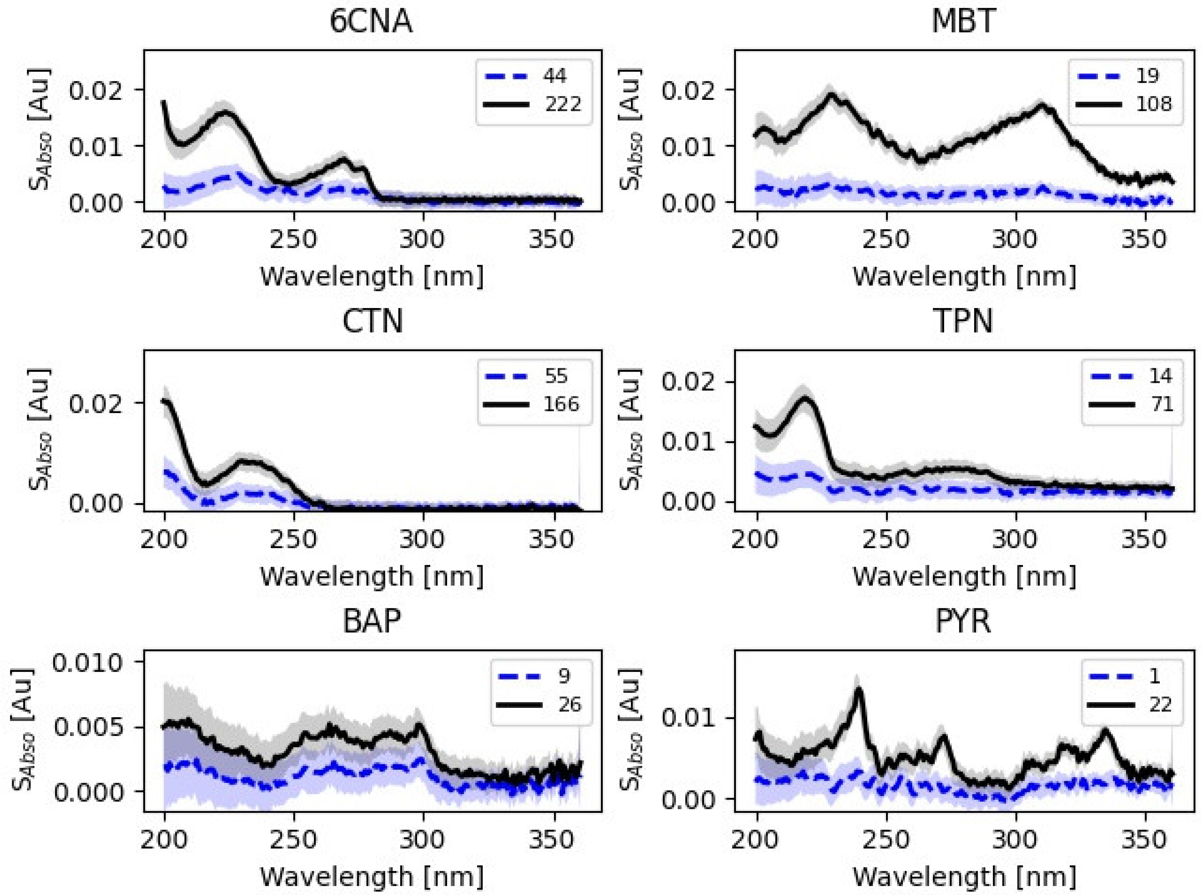
The sensitivity to detection of changes in water quality was tested by the addition of the six contaminants listed in
Section 2.1. S
Abso spectra are shown in
Figure 2. Because 6CNA, MBT, and CTN are not fluorescent, their presence in water will manifest itself via changes to the absorbance spectra. The signal of 254/360 fluorescence was detected for TPN and PYR and of 375/460 fluorescence for BAP. Detectable concentrations of TPN, PYR and BAP using fluorometers are much lower than the smallest detectable signal for UV-spec. Their absorbance spectra can, however, be valuable in identifying the cause of anomalies in an event with sufficiently high concentrations of substances.
3.2. Performance of Anomaly Detection
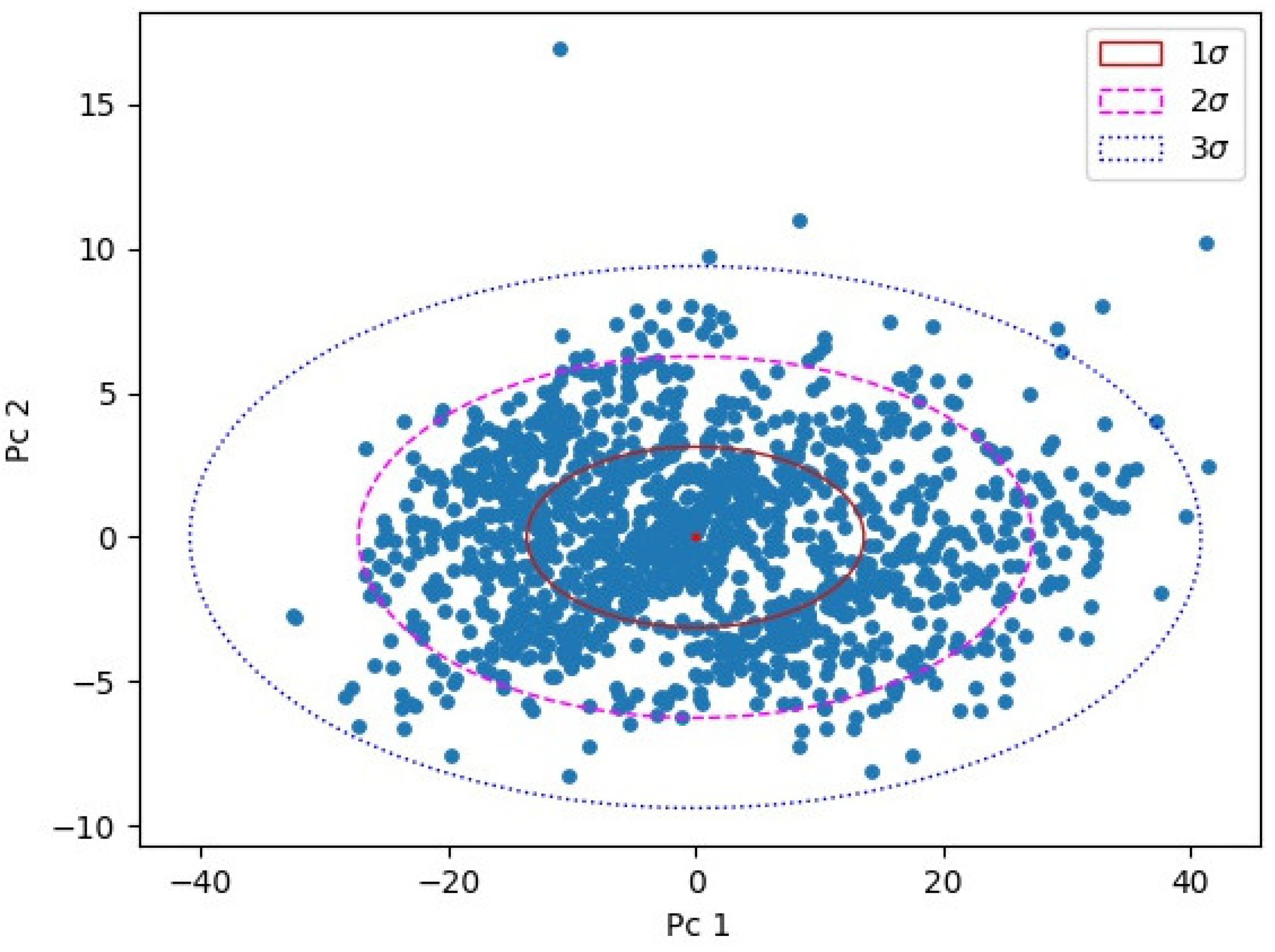
The development of the anomaly detection system is purely based on the baseline data. Given that fluorescence data are normally distributed, we used the Monte Carlo technique to enhance statistics for fluorescence data such that all baseline data had an equal number of points. These data were averaged over 10 min interval. Resulting baseline data statistics comprised 2631 points. Data were split into two equal size samples: a training set and a test set. The training set was used to fit PCA transformation parameters for absorbance baseline, which were then applied to the test set. The first five PCs explain 99.4% of variance in the data. The training set was subsequently used to extract the μ and σ parameters of the multivariate gaussian distribution.
The test set was used to evaluate performance.
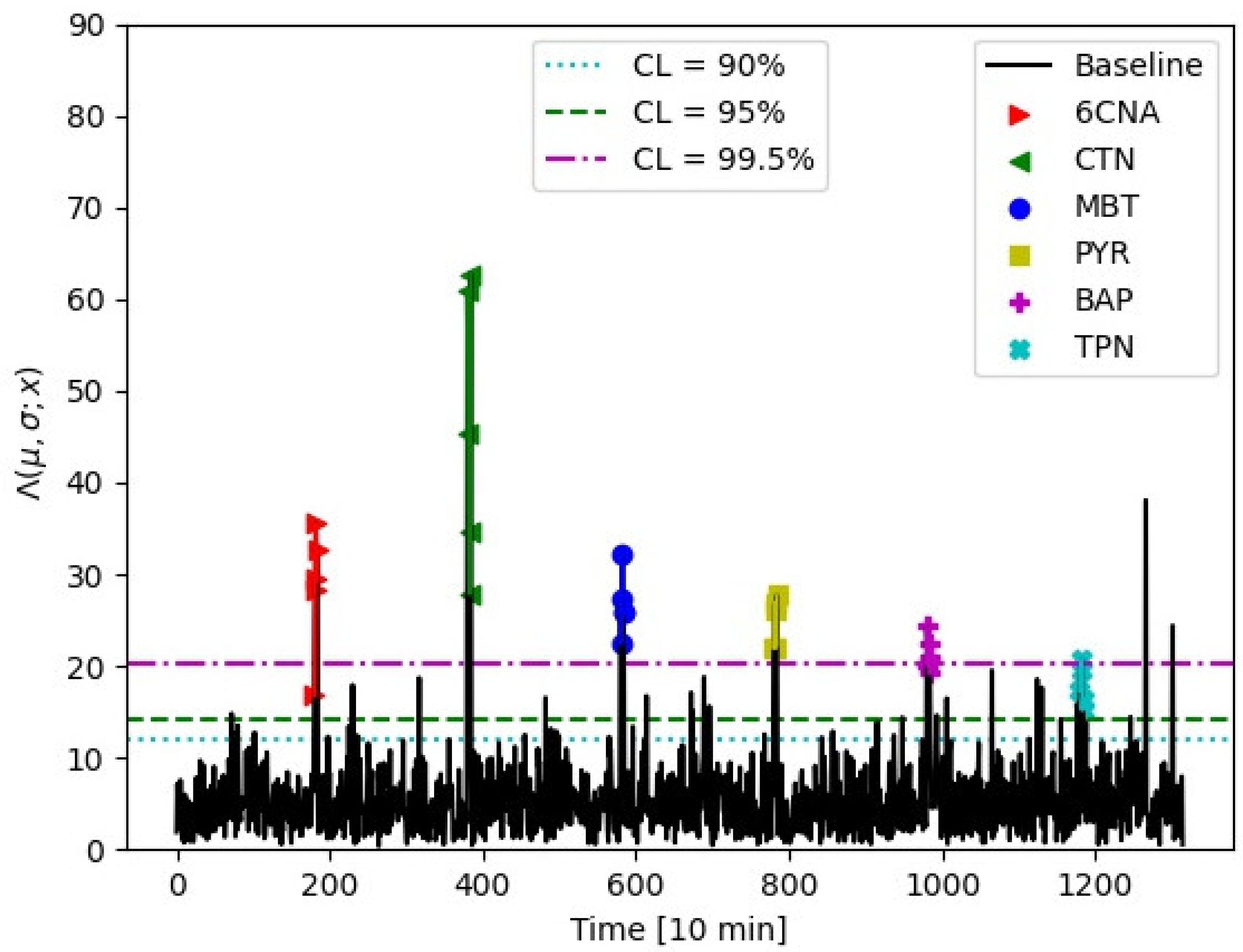
Figure 3 shows the leading two PCs for the test set with two-dimensional confidence ellipsoids overlayed. Parameters for ellipsoids were estimated in the training set. Log-likelihood ratio was used to project the seven-dimensional ellipsoid into the one-dimensional anomaly estimator, as explained in
Section 2.4. Our anomaly estimator can be equated to the critical values of χ
2 distribution for seven degrees of freedom. The concentrations applied and shown in
Figure 4 were 6CNA 44 μg/L, MBT 18 μg/L, CTN 56 μg/L, TPN 1.5 μg/L, PYR 0.3/L, and BAP 0.15 μg/L. It should be stressed that the achieved limits in anomaly detection are indicative. For real time monitoring, it is possible to rely on several consecutive anomalous events instead of a single event firing an alarm. Exact limits will, therefore, depend on applications, the rate of acceptable false positive alarms, and false negative misses as well as the integration level with anomaly identification described in the next section.
3.3. Performance of Anomaly Identification
To build the anomaly identification system, we used the same baseline data as the anomaly detection procedure, which are described in
Section 3.2. Baseline data were split into a test set and a training set. Both the training set and the test data were split into seven categories of equal size: one for baseline and one for each of the six chemicals of interest. The overlayed signals had the same concentrations as those in
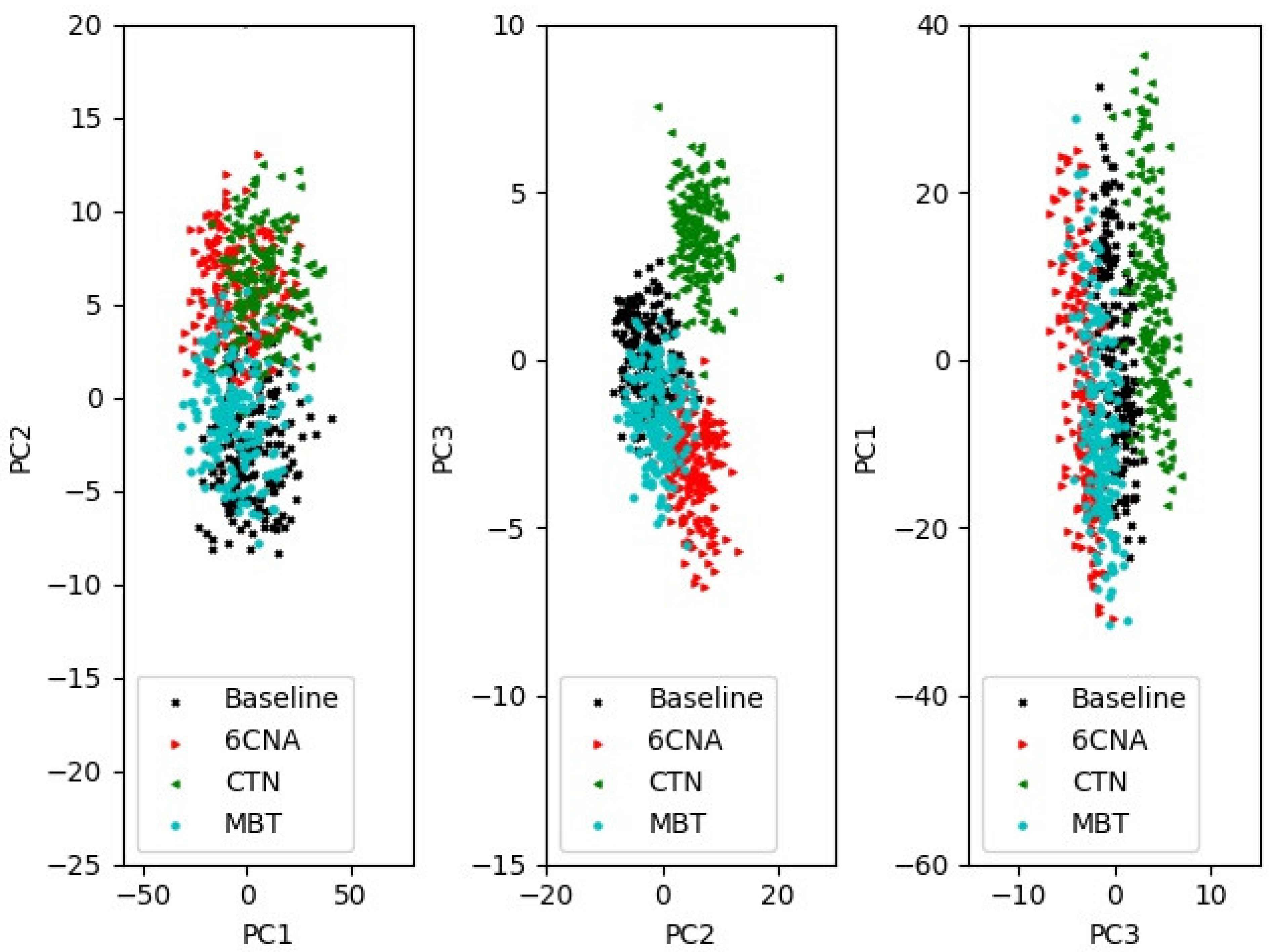
Section 3.2. PCA transformation parameters were extracted by fitting the train set. The leading three PCs are shown in
Figure 5.
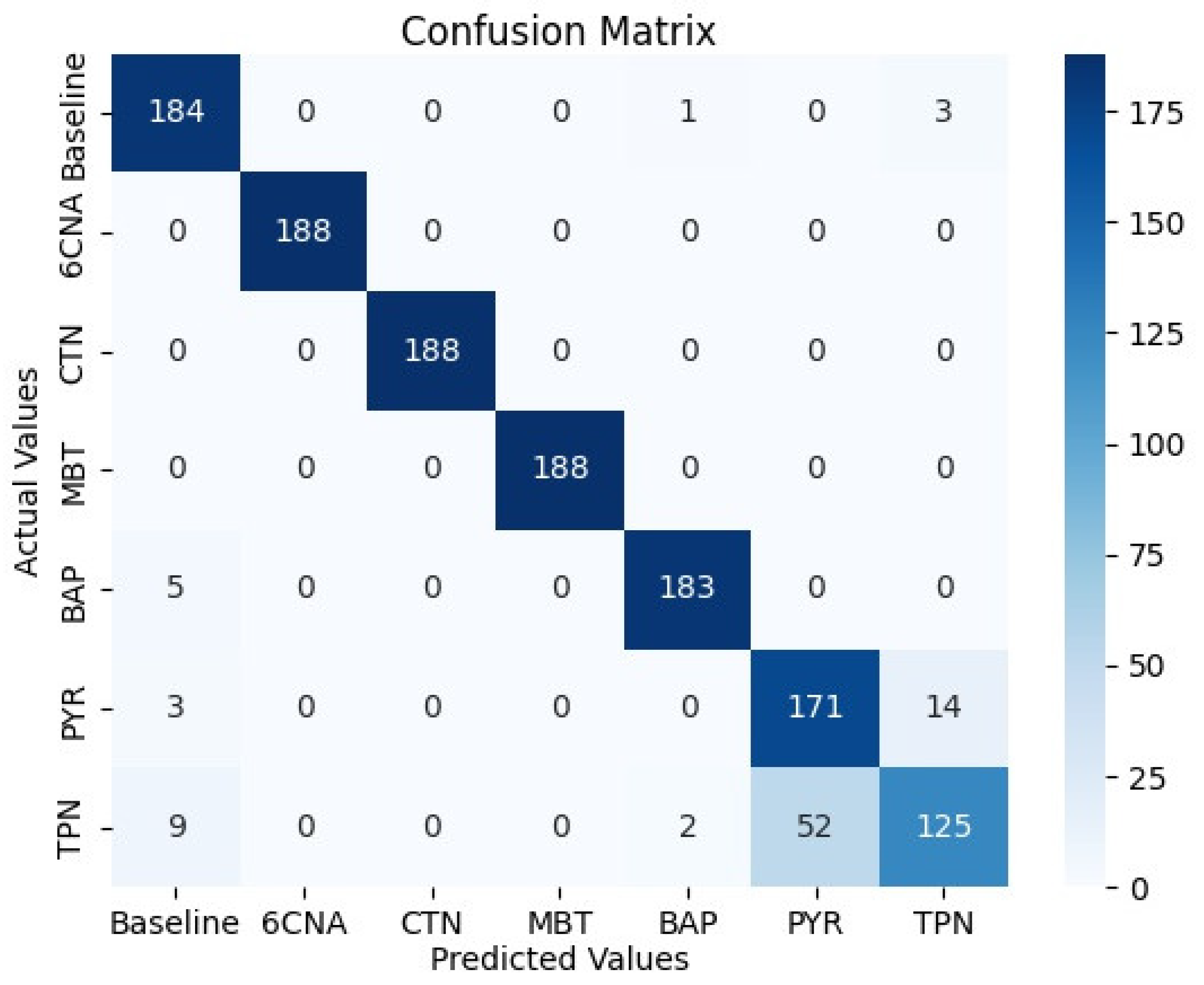
We trained a multinomial LR to recognize the six chemicals. The confusion matrix for LR prediction based on the test set is shown in
Figure 6. It should be noted that the LR performs better than the anomaly detection technique for the three chemicals that are characterized by more than one feature (five PCs) (that is, those that are not fluorescent). This is consistent with expectations that ML tools provide improvements in the description of complex data. BAP is distinguished from PYR and TPN based on the difference in the fluorescence wavelength. The detection of PYR and TPN relies upon the same property; therefore, mixing between them is expected. There was a small difference in concentrations between the two chemicals, leading to a small difference in fluorescence values. Therefore, a certain distinction between them was picked up by the model. This is, however, an artifact.
The anomaly identification tool can be coupled with anomaly detection to improve the ability to detect pollutants. It should be stressed that this improvement will occur only for contaminants known to the model.
4. Discussion
The goal is that sensors are applied as part of an online and real-time monitoring and control system. Such a system would be designed to proceed beyond conventional pollutants and water-quality measurements. This is performed to better cater to potential risks from any one of the hundreds of thousands of chemicals in use today that could pose a challenge to water quality. Previous studies in this field only focused primarily on traditional water-quality parameters, and there is extensive literature on AI systems for this purpose [
19]. The present study takes a broader view and is aimed at the vast chemical space and new emerging contaminants that may pose a risk to human health and the environment.
The optical sensors used in this study provide adequate sensitivity for the detection of a broader range of organic substances. The detection of anomalies arising from sub-1 µg/L concentrations of PAHs was shown, which is appropriate for the USEPA’s maximum contaminant level (MCL) in drinking water of 0.2 µg/L for BAP [
20]. Anomaly events were detectable for the other test substances at sub-50 µg/L concentrations. 6CNA is a degradation product of neonicotinoid insecticides imidacloprid and acetamiprid for which toxic effects were observed at 1 µM, equivalent to approximately 250 µg/L and belo [
21,
22]. MBT has a total allowable concentration (TAC) in the drinking water of 40 µg/L [
7].
Additional sensitivity gains may potentially be made by extending the timeframe and the amount of baseline data used to define the “normality” baseline. Baseline variability will, however, depend on the application area and where the sensors are deployed. It may also show seasonal trends or be correlated with external measures such as weather or turbidity. The inclusion of such baseline knowledge will provide for high sensitivities in anomaly detection. In this study, variability was averaged over 10 min intervals to reduce statistical fluctuations. This interval must be calibrated to fit the baseline variability scale specific to a given application area. This is true both in terms of amplitude and over time. While the calibration requirements of this system vary depending on its final application area, the overarching techniques remain the same. As a result, the technique could potentially be used in a variety of applications, including river monitoring, food and industrial process water, and a variety of other areas where water is used and reused.
While the development of Anomaly Detection requires only data on baseline variability over time, anomaly identification requires prior knowledge of the contaminants in order to train the model. The accuracy and breadth of applicability (scope) of the identification module would improve as the number of “known” pollutants or contaminants grows. For a proof of concept, we used only six substances from five chemical classes. This was useful for establishing effectiveness and sensitivity in this study, but these substances are only indicative of the potential for systems of this design.
The real-world application of this approach would involve iteration or continual improvement (re-training of the model) as new data become available. Anomaly detection could, for example, trigger an automated sample-collection process. This sample can be sent for thorough analysis via high-resolution mass spectrometry to identify the substance(s) causing the anomaly [
23]. Knowledge of the identified substance would then be used to update and re-train the anomaly identification model, and, thereby, expanding its “library” of known contaminants.
One acknowledged weakness of this study is that, for the sake of simplicity, we assumed only one chemical contaminant event at any given time. This implies that there are no interactions between target categories. While such an assumption may be correct in a wide range of situations, it is not always the case. The identification of several chemicals at a time is a multilabel classification problem in ML. Boosted decision tree (BDT) or Neural Network (NN) classifiers can be used in the anomaly identification system to perform this task. An increasingly challenging case arises when two separate and independent changes in the chemical composition of water counteract or negate the sensor signal from each other. This is less relevant for UV-spec because the absorbance signals show additive relations in the presence of multiple contaminants, but the quenching of fluorescence is a good example of a scenario that could be challenging. More research is needed to determine the impact of multiple sources on the effectiveness of anomaly detection and identification in such a scenario.
5. Conclusions
Changes in water quality can endanger human health and the environment. Changes can also have an impact on the quality of products and services that use water. Online and real-time monitoring and guidance can be critical to success.
Multi-sensor systems can be used to detect anomalies associated with chemical contamination in water in real-time. Optical sensors were used in this study as they provide sensitivity for a broad range of organic chemicals. This study used such sensor data to develop an AI for drinking water applications, but other sensors could be used to broaden the application’s area. While the exact combination of sensors may vary by application, the overarching technique remains the same. Sensor-based AI systems can be used in a variety of areas, including surface-water, urban runoff, food and industrial process water, aquaculture, and numerous areas where water is used and reused.
Author Contributions
Conceptualization, Z.C.R. and M.J.R.; methodology, Z.C.R.; formal analysis, Z.C.R.; investigation, Z.C.R. and C.U.S.; resources, Z.C.R. and M.J.R.; writing—original draft preparation, Z.C.R. and M.J.R.; writing—review and editing, Z.C.R., M.J.R., C.U.S. and Y.L.; visualization, Z.C.R.; funding acquisition, Y.L. All authors have read and agreed to the published version of the manuscript.
Funding
This work has been supported by Sino-Norwegian Cooperation Program on Hazardous Chemicals Relevant Environmental Convention Capacity Building (SINOCHEM, CHN-2150, 18/0014).
Informed Consent Statement
Not applicable.
Data Availability Statement
The data presented in this study are available upon request from the corresponding author.
Acknowledgments
We would like to thank Simen Stene from NIVA for practical help with the experimental setup.
Conflicts of Interest
The authors declare no conflict of interest.
Appendix A
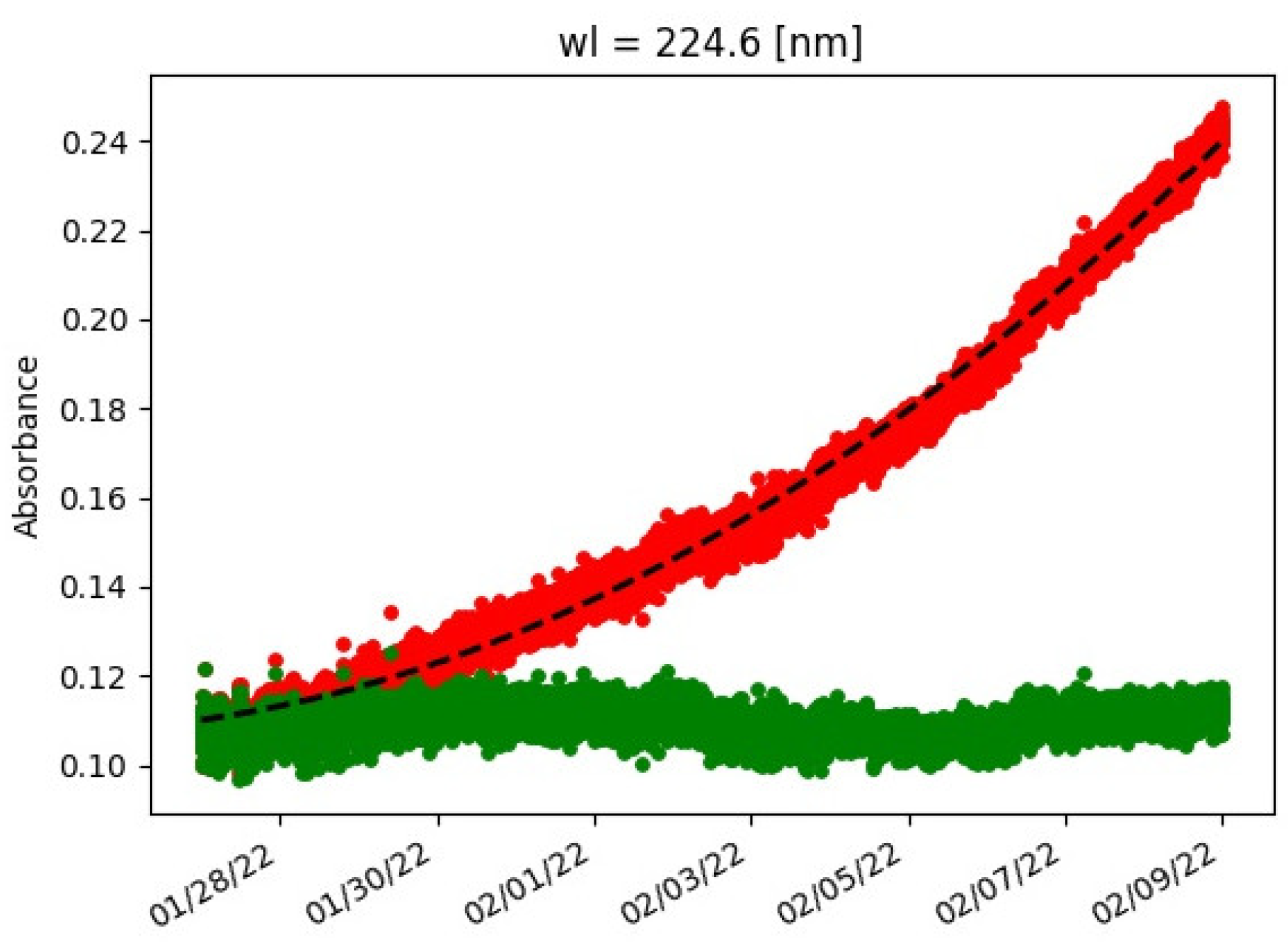
Uncontaminated UV-spec data after a couple of days of data collection showed a rapid increase in absorbance as a function of time. This was explained by biofouling accumulating on the lens. To correct for this effect, a second-order polynomial was fitted to the data, and the estimated trend was subtracted from the data. This is shown in
Figure A1 for a selected wavelength. This procedure was applied per wavelength.
Figure A1.
Absorbance as a function of time for a selected wavelength. Red denotes data with biofouling, black dashed line fitted second-order polynomial and green corrected data.
Figure A1.
Absorbance as a function of time for a selected wavelength. Red denotes data with biofouling, black dashed line fitted second-order polynomial and green corrected data.
References
- Riggi, E.; Friedman, J.; Schrijver, L.W.; Mayer, M.S.; Long, Y. Global Online Stakeholder Consultation: Themes for Interactive Dialogues. In Proceedings of the United Nations 2022 Water Conference; UN: New York, NY, USA, 2022. [Google Scholar]
- Storey, M.V.; van der Gaag, B.; Burns, B.P. Advances in online drinking water quality monitoring and early warning systems Author links open overlay panel. Water Res. 2011, 45, 741–747. [Google Scholar] [CrossRef] [PubMed]
- Williams, A.J.; Grulke, C.M.; Edwards, J.; McEachran, A.D.; Mansouri, K.; Baker, N.C.; Patlewicz, G.; Shah, I.; Wambaugh, J.F.; Judson, R.S. The CompTox Chemistry Dashboard—A Community Data Resource for Environmental Chemistry. J. Cheminform. 2017, 9, 1–27. [Google Scholar] [CrossRef] [PubMed]
- Spangenberg, M.; Bryant, J.I.; Gibson, S.J.; Mousley, P.J.; Ramachers, Y.; Bell, G.R. Ultraviolet absorption of contaminants in water. Sci. Rep. 2021, 11, 3682. [Google Scholar] [CrossRef] [PubMed]
- Sorensen, J.P.R.; Vivanco, A.; Ascott, M.J.; Gooddy, D.C.; Lapworth, D.J.; Read, D.S.; Rushworth, C.M.; Bucknall, J.; Herbert, K.; Karapanos, I. Online fluorescence spectroscopy for the real-time evaluation of the microbial quality of drinking water. Water Res. 2018, 137, 301–309. [Google Scholar] [CrossRef] [PubMed]
- Oslo Kommune Drikkevannskvalitet. Available online: https://www.oslo.kommune.no/vann-og-avlop/drikkevannskvalitet/ (accessed on 2 May 2022).
- Whittaker, M.H.; Gebhart, A.M.; Miller, T.C.; Hammer, F. Human health risk assessment of 2-mercaptobenzothiazole in drinking water. Toxicol. Ind. Health 2004, 20, 149–163. [Google Scholar] [CrossRef] [PubMed]
- Chen, C.; Kostakis, C.; Gerber, J.P.; Tscharke, B.J.; Irvine, R.J.; White, J.M. Towards finding a population biomarker for wastewater epidemiology studies. Sci. Total Environ. 2014, 487, 621–628. [Google Scholar] [CrossRef] [PubMed]
- Baker, A. Fluorescence Excitation−Emission Matrix Characterization of Some Sewage-Impacted Rivers. Environ. Sci. Technol. 2001, 35, 948–953. [Google Scholar] [CrossRef] [PubMed]
- Sorensen, J.P.R.; Sadhu, A.; Sampath, G.; Sugden, S.; Gupta, S.D.; Lapworth, D.J.; Marchant, B.P.; Pedley, S. Are sanitation interventions a threat to drinking water supplies in rural India? An application of tryptophan-like fluorescence. Water Res. 2016, 88, 923–932. [Google Scholar] [CrossRef] [PubMed] [Green Version]
- Grung, M.; Kringstad, A.; Bæk, K.; Allan, I.J.; Thomas, K.V.; Meland, S.; Ranneklev, S.B. Identification of non-regulated polycyclic aromatic compounds and other markers of urban pollution in road tunnel particulate matter. J. Hazard. Mater. 2017, 323, 36–44. [Google Scholar] [CrossRef] [PubMed]
- TriOS. TriOS OPUS. Available online: https://www.trios.de/en/opus.html (accessed on 2 May 2022).
- TriOS. TriOS enviroFlu. Available online: https://www.trios.de/en/enviroflu.html (accessed on 5 February 2022).
- TriOS. TriOS matrixFlu VIS. Available online: https://www.trios.de/en/matrixflu-vis.html (accessed on 2 May 2022).
- TriOS. Wiper W55 V2. Available online: https://www.trios.de/en/wiper.html (accessed on 2 May 2022).
- Pedregosa, F.; Varoquaux, G.; Gramfort, A.; Michel, V. Scikit-learn: Machine Learning in Python. J. Mach. Learn. Res. 2011, 12, 2825–2830. [Google Scholar]
- Press, W.H.; Teukolsky, S.A.; Vetterling, W.T.; Flannery, B.P. Press, Numerical Recipes 3rd Edition: The Art of Scientific Computing, 3rd ed.; Cambridge University Press: Cambridge, UK, 2007. [Google Scholar]
- Bonaccorso, G. Machine Learning Algorithms; Packt Publishing: Birmingham, UK, 2018. [Google Scholar]
- Ighalo, J.O.; Adeniyi, A.G.; Marques, G. Artificial intelligence for surface water quality monitoring and assessment: A systematic literature analysis. Modeling Earth Syst. Environ. Vol. 2021, 7, 669–681. [Google Scholar] [CrossRef]
- National Primary Drinking Water Regulations. Available online: https://www.epa.gov/ground-water-and-drinking-water/national-primary-drinking-water-regulations (accessed on 26 June 2022).
- Health, U.D. Risk Assessment. Available online: https://www.health.state.mn.us/communities/environment/risk/docs/guidance/gw/imidasumm.pdf (accessed on 26 June 2022).
- Kimura-Kuroda, J.; Komuta, Y.; Kuroda, Y.; Hayashi, M.; Kawano, H. Nicotine-Like Effects of the Neonicotinoid Insecticides Acetamiprid and Imidacloprid on Cerebellar Neurons from Neonatal Rats. PLoS ONE 2012, 7, e32432. [Google Scholar] [CrossRef] [PubMed]
- Samanipour, S.; Kaserzon, S.; Vijayasarathy, S.; Jiang, H.; Choi, P.; Reid, M.J.; Mueller, J.F.; Thomas, K.V. Machine learning combined with non-targeted LC-HRMS analysis for a risk warning system of chemical hazards in drinking water: A proof of concept. Talanta 2019, 195, 426–432. [Google Scholar] [CrossRef] [PubMed]
| Publisher’s Note: MDPI stays neutral with regard to jurisdictional claims in published maps and institutional affiliations. |
© 2022 by the authors. Licensee MDPI, Basel, Switzerland. This article is an open access article distributed under the terms and conditions of the Creative Commons Attribution (CC BY) license (https://creativecommons.org/licenses/by/4.0/).


