
Velocity Measurements in Highly Aerated Flow on a Stepped Chute without Sidewall Constraint Using a BIV Technique

 , , , and
Abstract
:1. Introduction
2. Experimental Set-Up
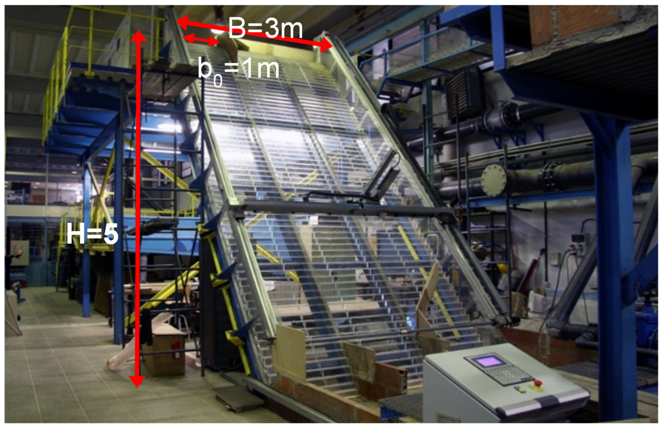
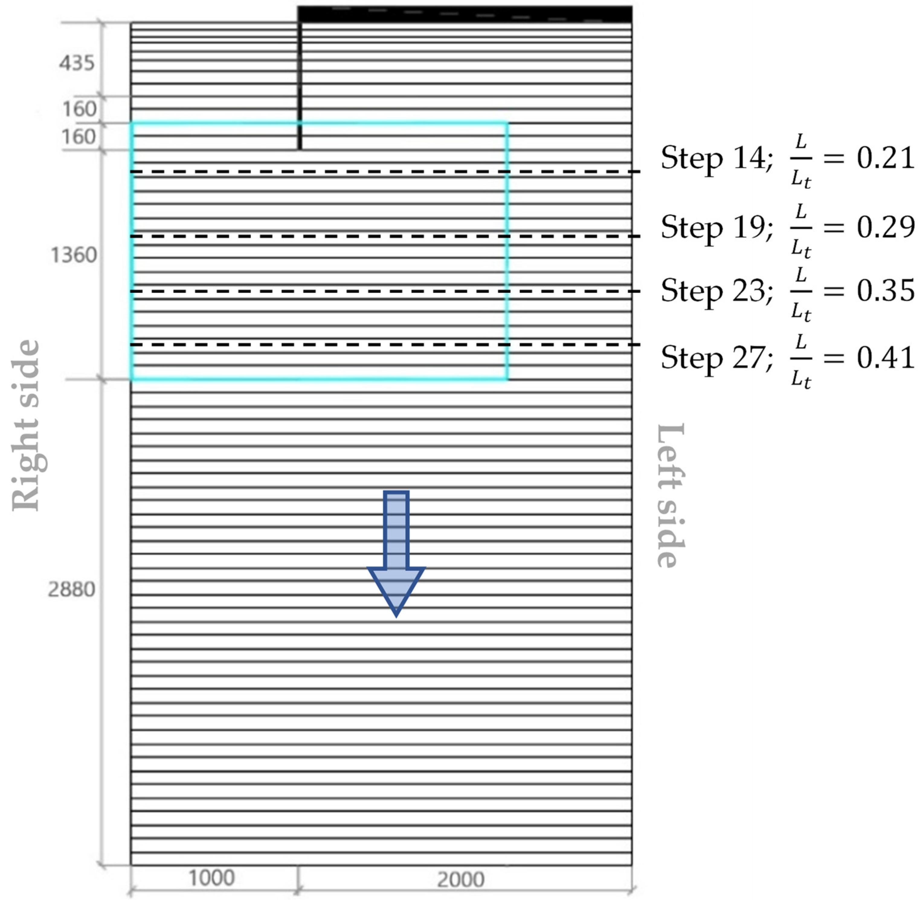
2.1. Physical Model
2.2. Video Recording Apparatus
3. Methodology
3.1. Position of the Camera
3.1.1. Frontal View
3.1.2. Lateral View
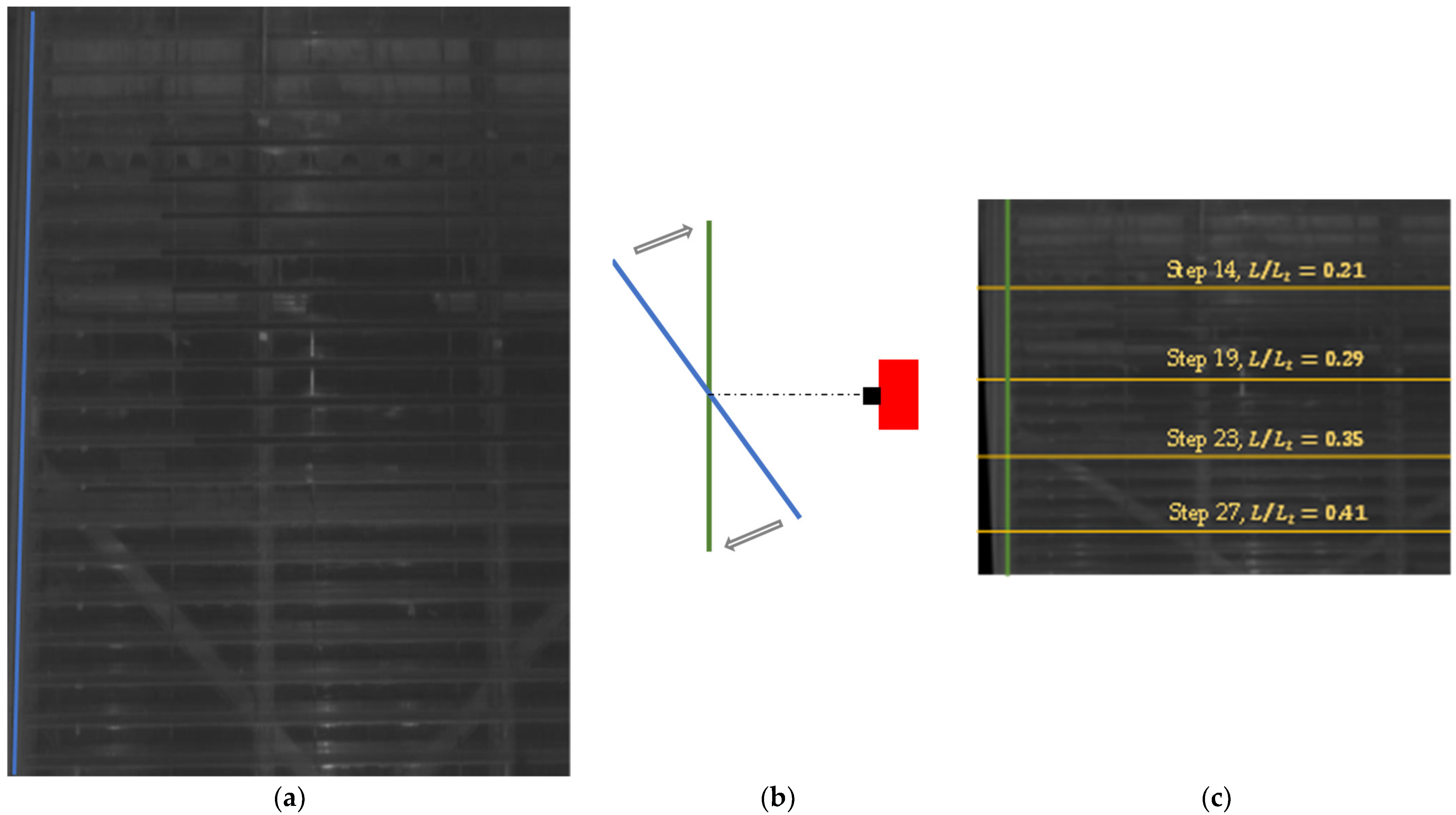
3.2. Folding Images
3.2.1. Frontal View
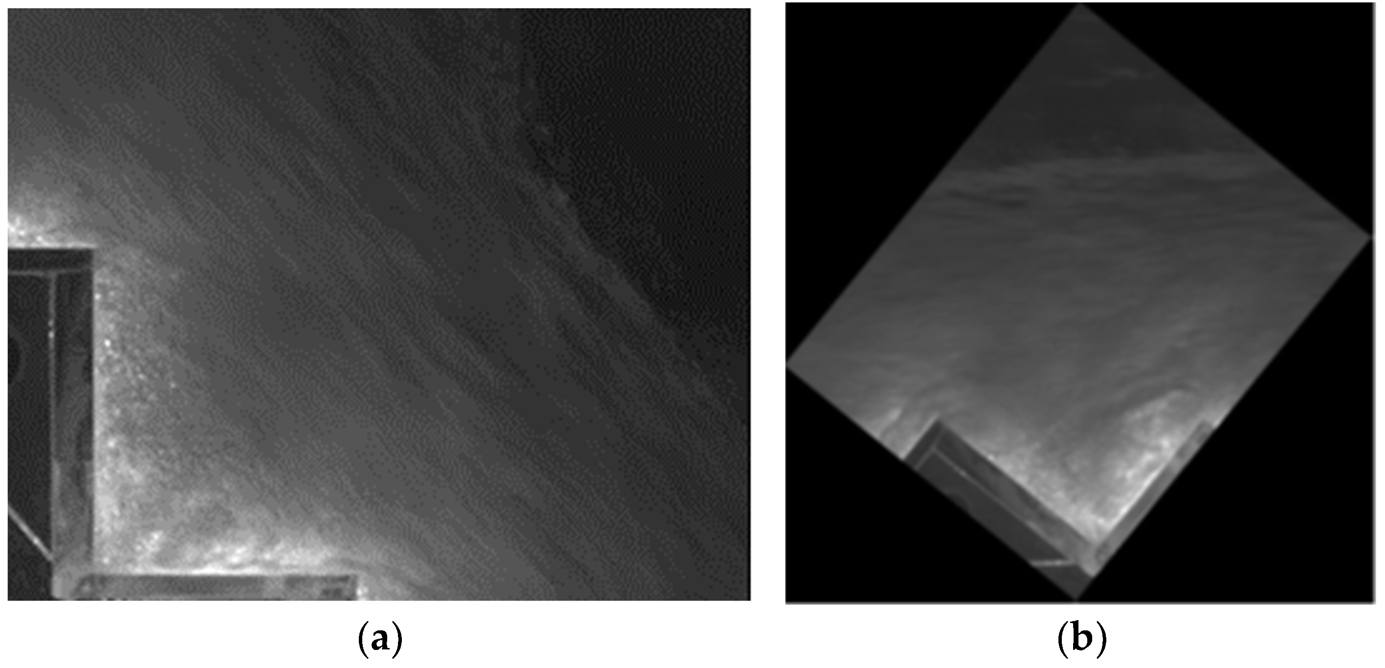
3.2.2. Lateral View
3.3. Preprocessing Frames in PIVlab
3.4. Interrogation Areas in PIVlab
3.4.1. Frontal View Velocity Field
3.4.2. Lateral View Velocity Field
4. Results and Discussion
4.1. Post-Processing of the Velocity Fields
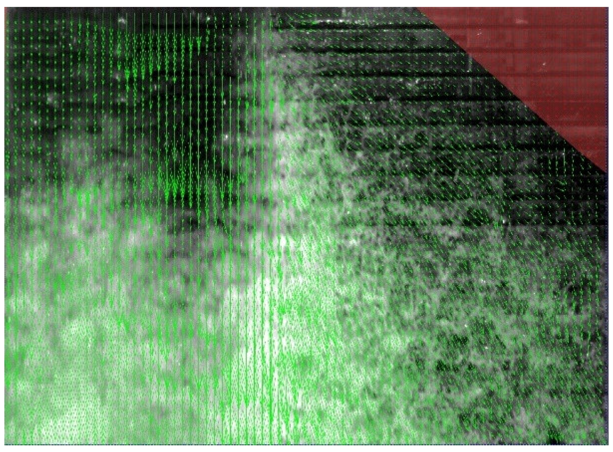
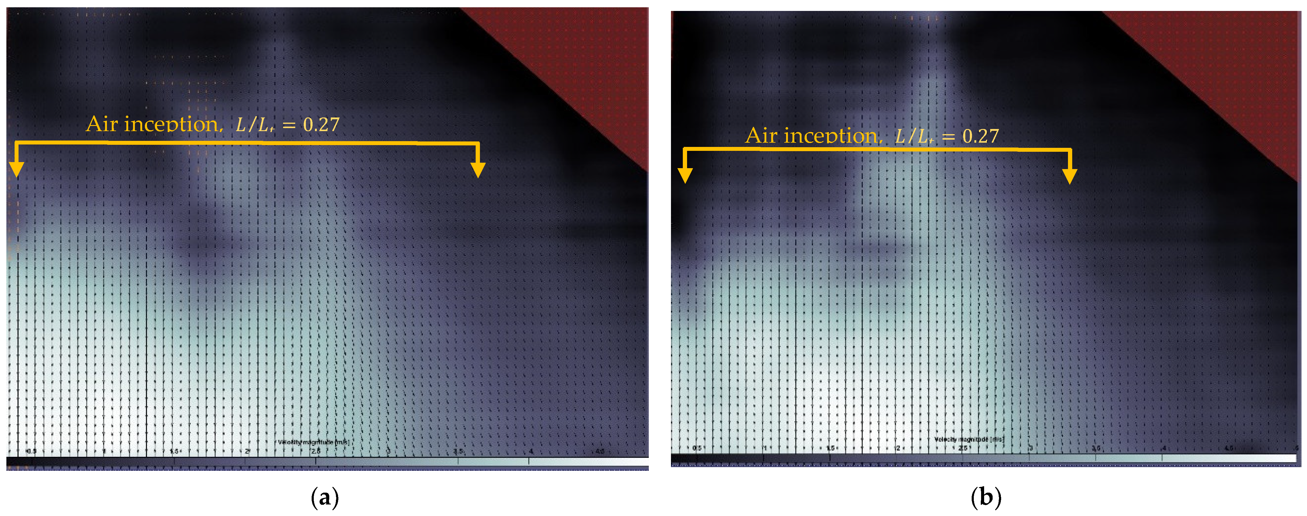
4.2. Frontal View Velocity Field
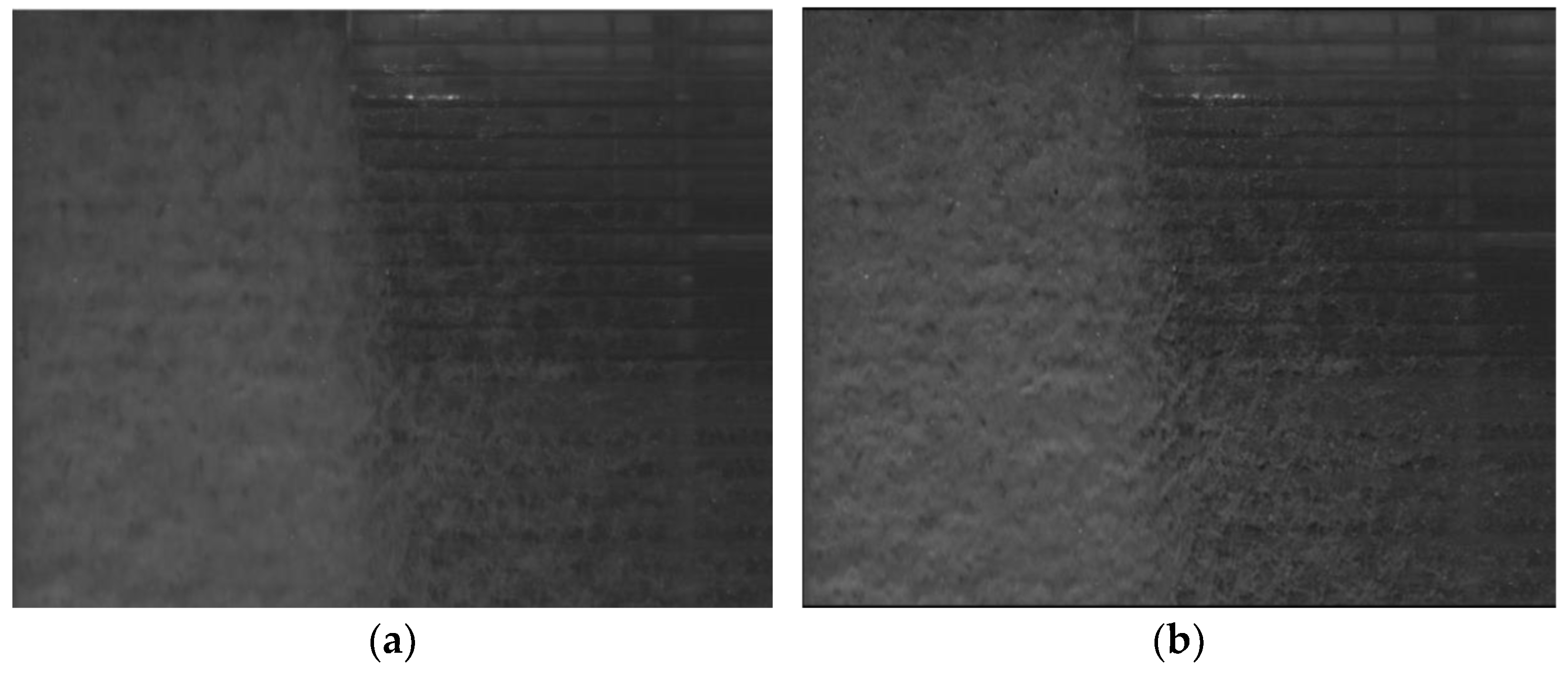
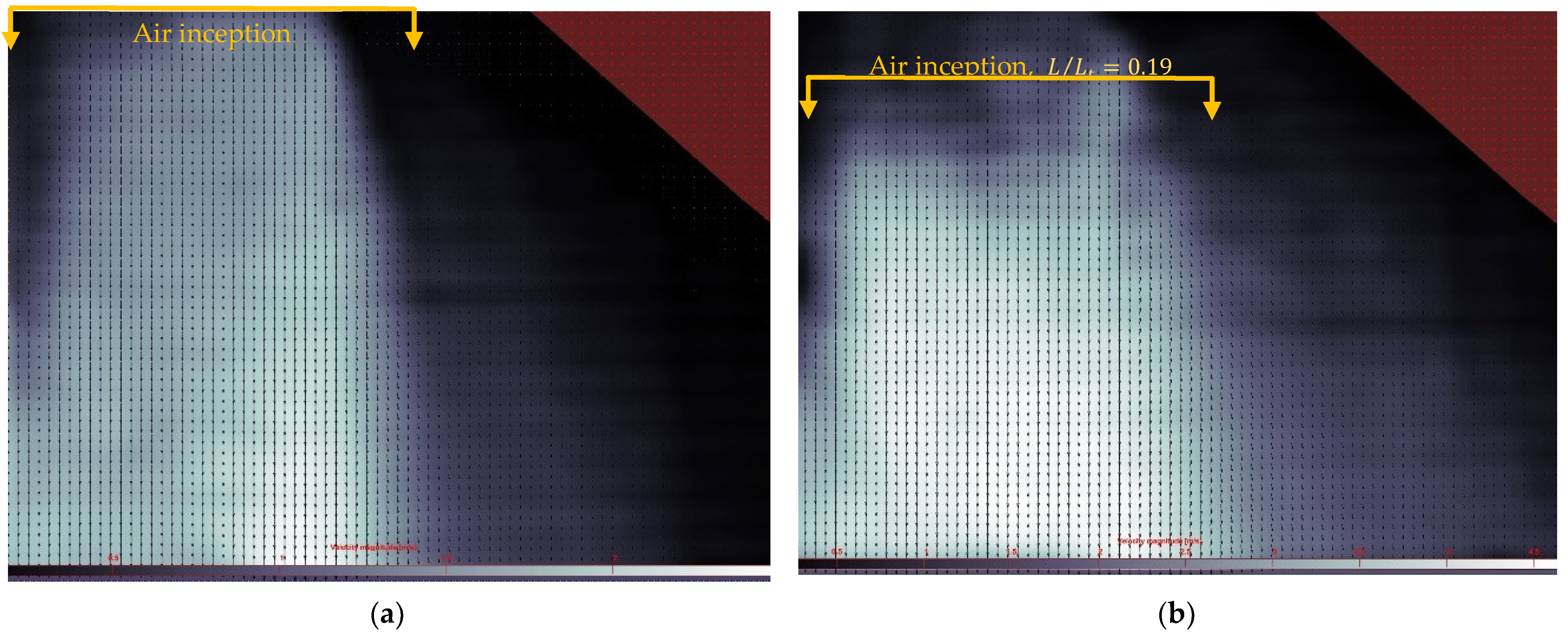
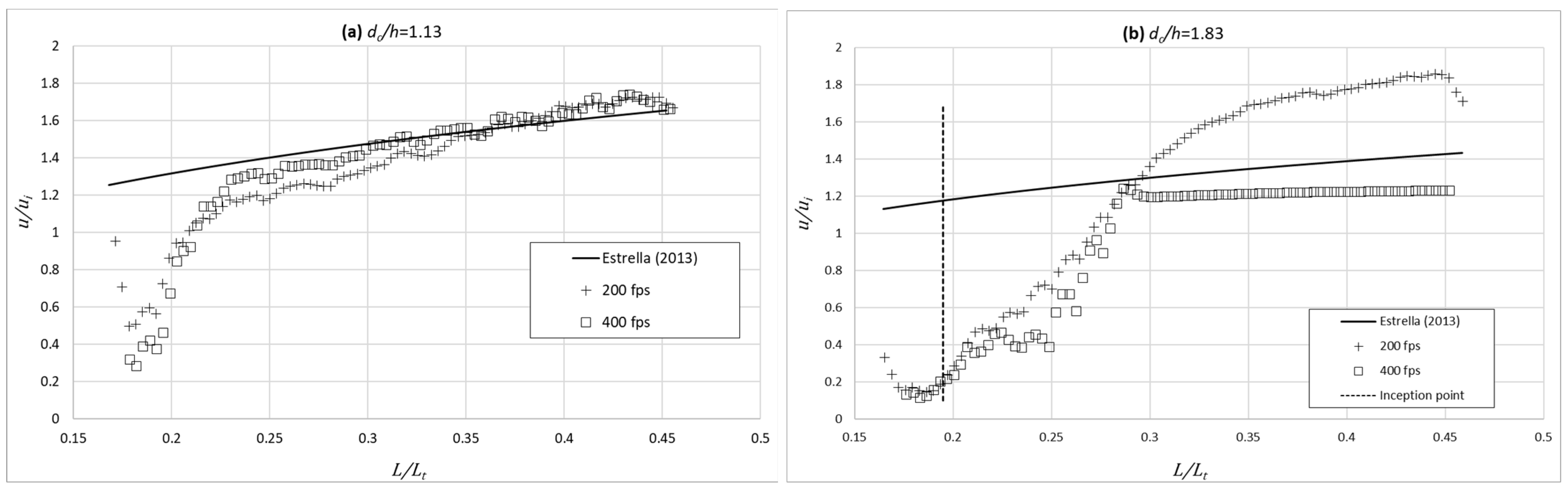
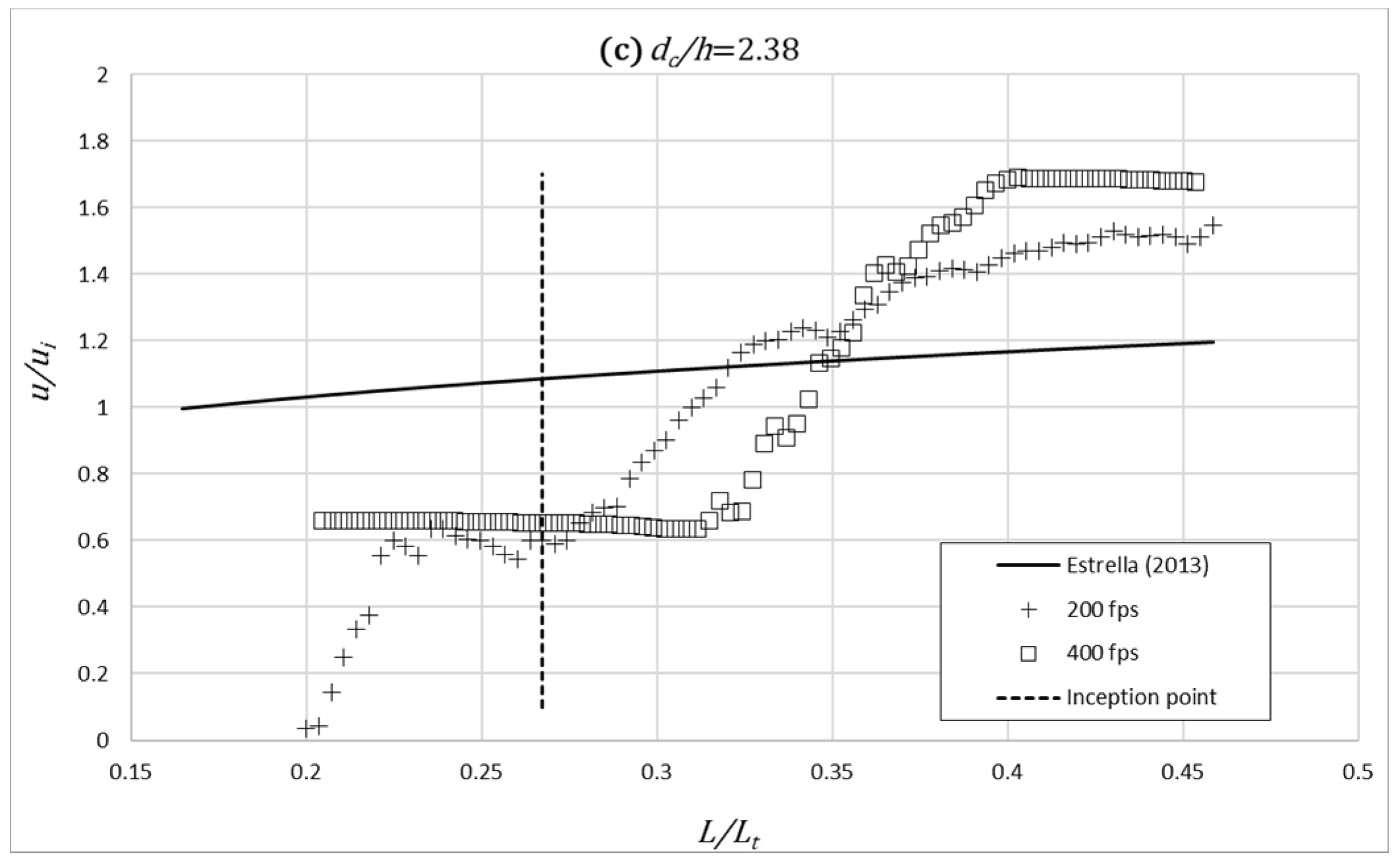
- Shortly downstream of the point of inception, where air is not fully entrained, a dark zone is observed. That causes a reduction in the estimation of the correlations between consecutive frames and, therefore, generates a greater dispersion and errors in the velocity measurement. In this area, it is observed that the estimation of the dimensionless velocity () is, in general, significantly underestimated with respect to that obtained by [17,45] in the same physical model.
- Downstream of the previous dark zone, there is a bright area that coincides with the area where aeration inception has already occurred. This brightness allows a better tracking of correlations between consecutive images. That is, surface air acts as an acceptable flow tracer for velocity estimation. However, an overall tendency of overestimation of the dimensionless velocity () is noticeable sufficiently downstream of the point of inception, namely for the largest dimensionless flow rate.
- Improving the lighting of the darkest area is detrimental to creating brightness saturation in the area where the air has already reached the surface. This makes it very difficult to find optimal lighting for both regions. Additional research should be developed on this topic.
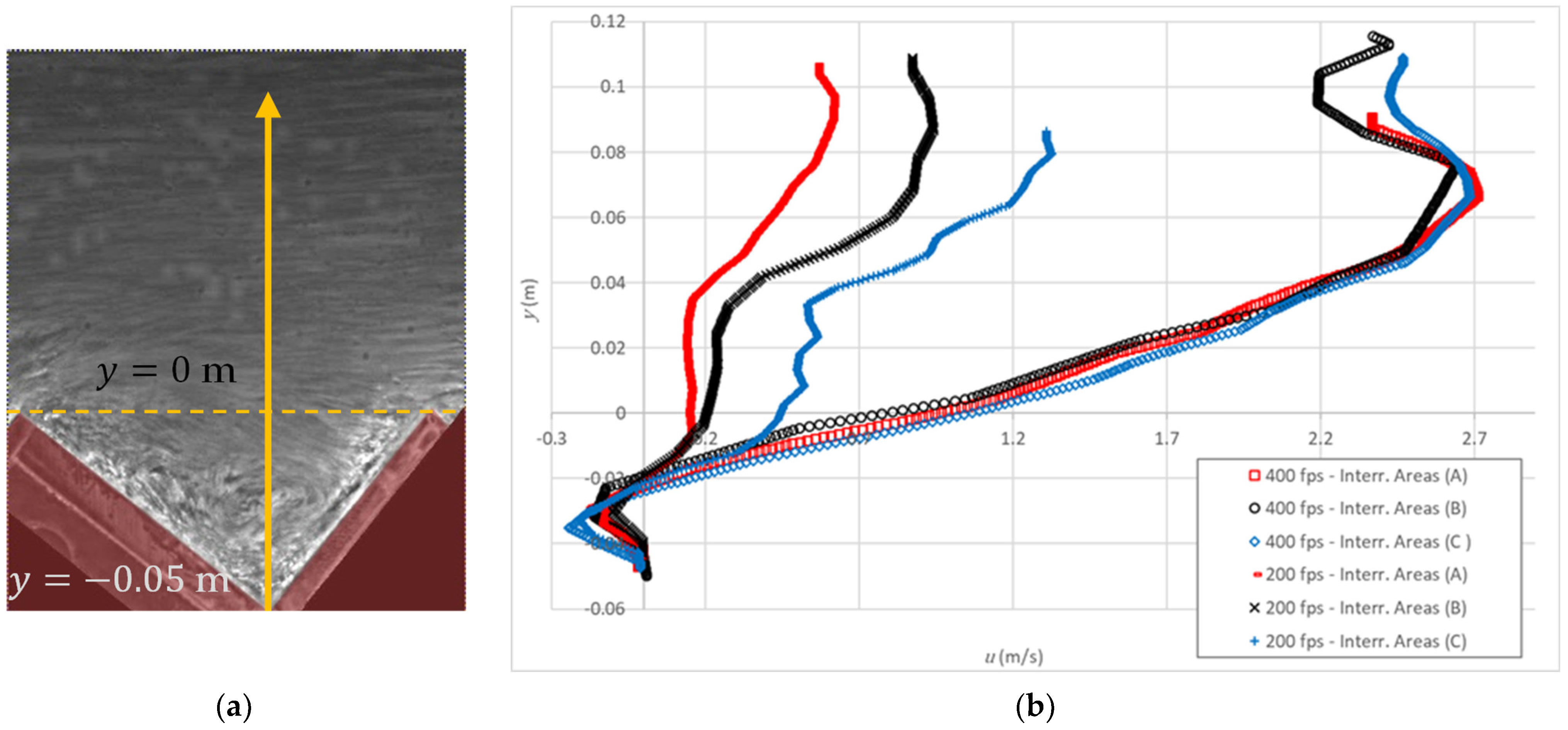
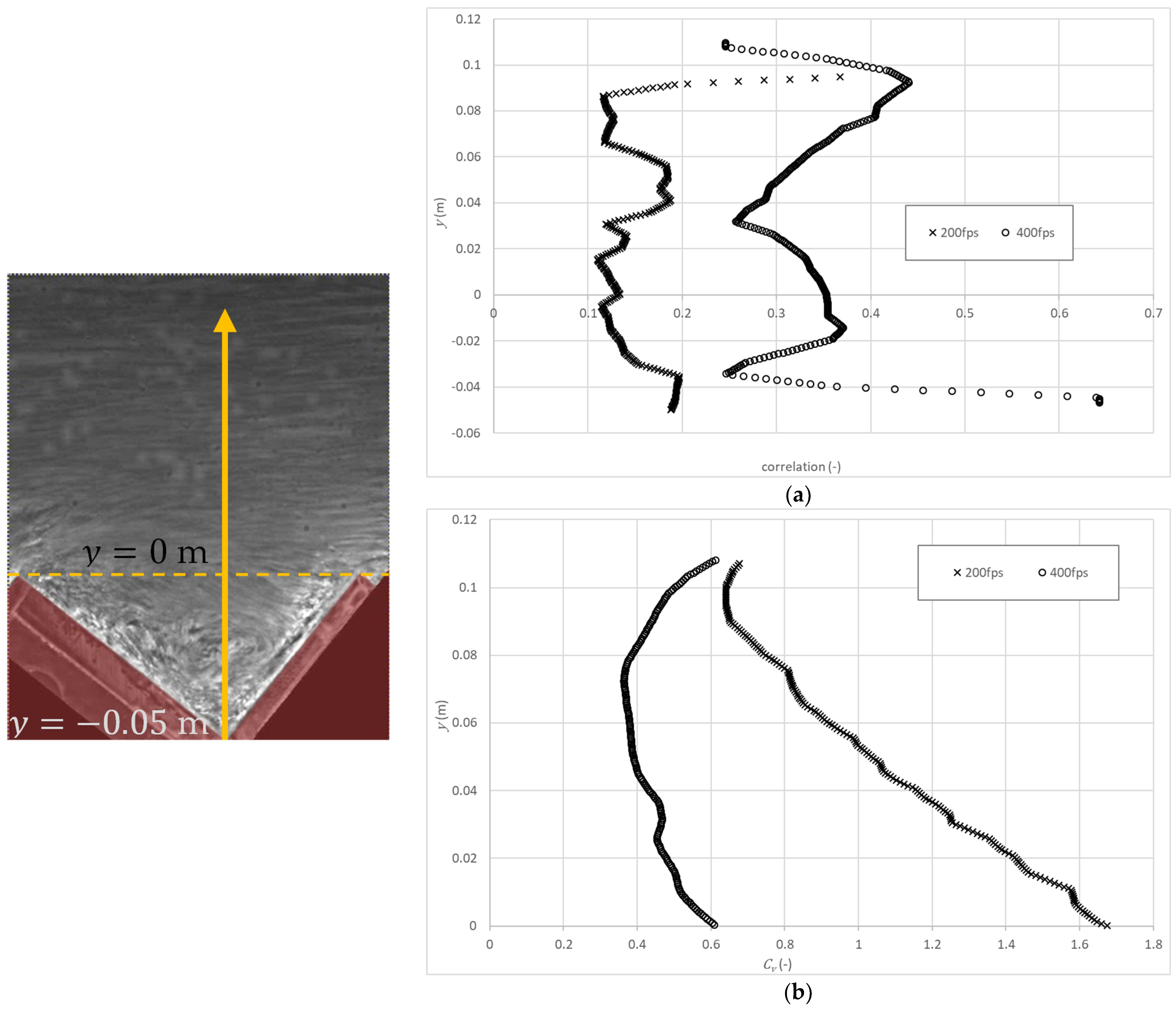
4.3. Lateral View Velocity Profile
5. Conclusions
- Image pre-processing is considered necessary to improve contrast so as to highlight the presence of air within the flow. In the present study, a rotation of images for both frontal and lateral analysis and a CLAHE filter were applied. Overall, for both views, the results were not influenced by the size of the interrogation areas.
- PIVlab appears to be a valid tool to estimate free-surface velocities from frontal view measurements, for highly aerated flows, using air bubbles as tracers. Correlations between consecutive frames are acceptable, regardless of the image acquisition rate. However, inaccurate estimations were obtained shortly downstream of the inception point, in the partially aerated region.
- Free-surface velocities, obtained from frontal view measurements, tend to increase downstream of the inception point, showing an increasing transverse component due to the lack of a lateral sidewall. For small dimensionless discharges and sufficiently downstream of the point of inception, the free-surface velocity compares relatively well with the air–water interfacial velocity previously obtained with a double-tip fiber optical probe in the same facility. However, for the largest dimensionless discharges, significant differences were obtained regardless of the image acquisition rate.
- The velocity profiles estimated from the lateral view measurements are practically independent of the size of the interrogation area for 400 fps. In contrast, for 200 fps, the velocities are markedly dependent on the size of the interrogation area, being significantly smaller than those obtained for 400 fps.
- The velocity profiles along the normal to the pseudo-bottom far downstream of the inception point, for 400 fps, are in reasonable agreement with air–water interfacial velocity profiles previously obtained in the same chute, except in the external flow zone, where larger differences were obtained, possibly due to poor lighting, yielding low correlations between consecutive frames. Providing adequate lighting of the area of interest is judged of relevance to improve the performance of air as a flow tracer.
Author Contributions
Funding
Institutional Review Board Statement
Informed Consent Statement
Data Availability Statement
Conflicts of Interest
Notations
| transverse distance from the right wall of the chute (m) | |
| chute width at the upstream end (m) | |
| coefficient of variation (-) | |
| critical depth (m) | |
| characteristic flow depth relative to 0.90 air concentration (m) | |
| gravitational acceleration (m/s2) | |
| step height (m) | |
| step roughness height (m) | |
| streamwise distance along the chute to the outer edge of the step (m) | |
| total length of the chute (m) | |
| unit discharge at the chute entrance (m2/s) | |
| coordinate perpendicular to and starting at the pseudo-bottom (m) | |
| time (s) | |
| velocity (m/s) | |
| velocity at (m/s) | |
| velocity at the inception point (m/s) |
References
- Chanson, H. The Hydraulics of Stepped Chutes and Spillways; Balkema: Lisse, The Netherlands, 2002; ISBN 9058093522. [Google Scholar]
- Chanson, H.; Bung, D.B.; Matos, J. Stepped Spillways and Cascades. In Energy Dissipation in Hydraulic Structures; Chanson, H., Ed.; CRC Press: Boca Raton, FL, USA, 2015; p. 20. ISBN 9780429225994. [Google Scholar]
- Frizell, K.W.; Frizell, K.H. Guidelines for the Hydraulic Design of Stepped Spillways; Hydraulic Laboratory Report HL-2015-06; Bureau of Reclamation: Denver, CO, USA, 2015. [Google Scholar]
- Hager, W.H.; Schleiss, A.J.; Boes, R.M.; Pfister, M. Hydraulic Engineering of Dams; CRC Press: London, UK, 2020; ISBN 9780203771433. [Google Scholar]
- Sánchez-Juny, M.; Dolz, J. Experimental Study of Transition and Skimming Flows on Stepped Spillways in RCC Dams: Qualitative Analysis and Pressure Measurements. J. Hydraul. Res. 2005, 43, 540–548. [Google Scholar] [CrossRef]
- Sánchez-Juny, M.; Bladé, E.; Dolz, J. Pressures on a Stepped Spillway. Pressions Sur Un Déversoir En Gradins. J. Hydraul. Res. 2007, 45, 505–511. [Google Scholar] [CrossRef]
- Sánchez-Juny, M.; Bladé, E.; Dolz, J. Analysis of Pressures on a Stepped Spillway. J. Hydraul. Res. 2008, 46, 410–414. [Google Scholar] [CrossRef]
- Amador, A.; Sánchez-Juny, M.; Dolz, J. Developing Flow Region and Pressure Fluctuations on Steeply Sloping Stepped Spillways. J. Hydraul. Eng. ASCE 2009, 135, 1092–1100. [Google Scholar] [CrossRef]
- André, S.; Matos, J.; Boillat, J.-L.; Schleiss, A. Energy Dissipation and Hydrodynamic Forces of Aerated Flow over Macro-Roughness Linings for Overtopped Embankment Dams. In Proceedings of the International Conference on Hydraulics of Dams and River Structures; Yazdandoost, F., Attari, J., Eds.; Taylor & Francis Group: Teheran, Iran, 2004; pp. 189–196. [Google Scholar]
- Tehrani, M.J.O.M.; Matos, J.; Pfister, M.; Schleiss, A.J. Bottom-Pressure Development Due to an Abrupt Slope Reduction at Stepped Spillways. Water 2022, 14, 41. [Google Scholar] [CrossRef]
- Matos, J.; Novakoski, C.K.; Ferla, R.; Marques, M.G.; Dai Prá, M.; Canellas, A.V.B.; Teixeira, E.D. Extreme Pressures and Risk of Cavitation in Steeply Sloping Stepped Spillways of Large Dams. Water 2022, 14, 306. [Google Scholar] [CrossRef]
- Frizell, K.W.; Renna, F.M.; Matos, J. Cavitation Potential of Flow on Stepped Spillways. J. Hydraul. Eng. 2013, 139, 630–636. [Google Scholar] [CrossRef]
- Boes, R.M.; Hager, W.H. Two-Phase Flow Characteristics of Stepped Spillways. J. Hydraul. Eng. 2003, 129, 661–670. [Google Scholar] [CrossRef]
- Pfister, M.; Hager, W.H. Self-Entrainment of Air on Stepped Spillways. Int. J. Multiph. Flow 2011, 37, 99–107. [Google Scholar] [CrossRef]
- Relvas, A.T.; Pinheiro, A.N. Velocity Distribution and Energy Dissipation along Stepped Chutes Lined with Wedge-Shaped Concrete Blocks. J. Hydraul. Eng. ASCE 2011, 137, 423–431. [Google Scholar] [CrossRef]
- Takahashi, M.; Ohtsu, I. Aerated Flow Characteristics of Skimming Flow over Stepped Chutes. J. Hydraul. Res. 2012, 50, 427–434. [Google Scholar] [CrossRef]
- Estrella, S.; Sánchez-Juny, M.; Bladé, E.; Dolz, J. Physical Modeling of a Stepped Spillway without Sidewalls. Can. J. Civ. Eng. 2015, 42, 311–318. [Google Scholar] [CrossRef]
- Ostad Mirza, M.J.; Matos, J.; Pfister, M.; Schleiss, A.J. Effect of an Abrupt Slope Change on Air Entrainment and Flow Depths at Stepped Spillways. J. Hydraul. Res. 2017, 55, 362–375. [Google Scholar] [CrossRef]
- Felder, S.; Pfister, M. Comparative Analyses of Phase-Detective Intrusive Probes in High-Velocity Air–Water Flows. Int. J. Multiph. Flow 2017, 90, 88–101. [Google Scholar] [CrossRef]
- Kramer, M.; Hohermuth, B.; Valero, D.; Felder, S. Best Practices for Velocity Estimations in Highly Aerated Flows with Dual-Tip Phase-Detection Probes; Elsevier Ltd.: Amsterdam, The Netherlands, 2020; Volume 126, ISBN 0000000310796. [Google Scholar]
- Terrier, S.; Pfister, M.; Schleiss, A.J. Performance and Design of a Stepped Spillway Aerator. Water 2022, 14, 153. [Google Scholar] [CrossRef]
- Hunt, S.L.; Kadavy, K.C.; Wahl, T.L.; Moses, D.W. Physical Modeling of Beveled-Face Stepped Chute. Water 2022, 14, 365. [Google Scholar] [CrossRef]
- Frizell, K.H.; Ehler, D.G.; Mefford, B.W. Developing Air Concentration and Velocity Probes for Measuring Highly-Aerated, High-Velocity Flow. In Proceedings of the Symposium on Fundamentals and Advancements in Hydraulic Measurements and Experimentation; ASCE: Reston, VA, USA, 1994; pp. 268–277. [Google Scholar]
- Matos, J.; Frizell, K.H. Air Concentration Measurements in Highly Turbulent Aerated Flow. In Environmental and Coastal Hydraulics: Protecting the Aquatic Habitat; Wang, S.S.Y., Carsten, T., Eds.; ASCE: Reston, VA, USA, 1997; Volume B, pp. 149–154. [Google Scholar]
- Matos, J.; Frizell, K.H. Air Concentration and Velocity Measurements on Self-Aerated Flow down Stepped Chutes. In Proceedings of the Joint Conference on Water Resource Engineering and Water Resources Planning and Management 2000, Minneapolis, MN, USA, 30 July–2 August 2000; American Society of Civil Engineers. Volume 104. [Google Scholar]
- Chamani, M.R.; Rajaratnam, N. Characteristics of Skimming Flow over Stepped Spillways. J. Hydraul. Eng. ASCE 1999, 126, 361–368. [Google Scholar] [CrossRef]
- Matos, J.; Meireles, I. Hydraulics of Stepped Weirs and Dam Spillways: Engineering Challenges, Labyrinths of Research. In Proceedings of the ISHS 2014—Hydraulic Structures and Society—Engineering Challenges and Extremes: Proceedings of the 5th IAHR International Symposium on Hydraulic Structures, Brisbane, Australia, 25–27 June 2014; pp. 127–134. [Google Scholar]
- Ohtsu, I.; Yasuda, Y. Characteristics of Flow Conditions on Stepped Channels. In Proceedings of the 27th IAHR Biennial Congress, San Francisco, CA, USA, 10–15 August 1997; pp. 583–588. [Google Scholar]
- Amador, A.; Sánchez-Juny, M.; Dolz, J. Characterization of the Nonaerated Flow Region in a Stepped Spillway by PIV. J. Fluids Eng. 2006, 128, 1266–1273. [Google Scholar] [CrossRef]
- Zhang, G.; Valero, D.; Bung, D.B.; Chanson, H. On the Estimation of Free-Surface Turbulence Using Ultrasonic Sensors. Flow Meas. Instrum. 2018, 60, 171–184. [Google Scholar] [CrossRef]
- Kramer, M.; Chanson, H.; Felder, S. Can We Improve the Non-Intrusive Characterization of High-Velocity Air–Water Flows? Application of LIDAR Technology to Stepped Spillways. J. Hydraul. Res. 2020, 58, 350–362. [Google Scholar] [CrossRef]
- Leandro, J.; Bung, D.B.; Carvalho, R. Measuring Void Fraction and Velocity Fields of a Stepped Spillway for Skimming Flow Using Non-Intrusive Methods. Exp. Fluids 2014, 55, 1732. [Google Scholar] [CrossRef]
- Bung, D.B.; Valero, D. Optical Flow Estimation in Aerated Flows. J. Hydraul. Res. 2016, 54, 575–580. [Google Scholar] [CrossRef]
- Zhang, G.; Chanson, H. Application of Local Optical Flow Methods to High-Velocity Free-Surface Flows: Validation and Application to Stepped Chutes. Exp. Therm. Fluid Sci. 2018, 90, 186–199. [Google Scholar] [CrossRef]
- Kramer, M.; Chanson, H. Optical Flow Estimations in Aerated Spillway Flows: Filtering and Discussion on Sampling Parameters. Exp. Therm. Fluid Sci. 2019, 103, 318–328. [Google Scholar] [CrossRef]
- Lopes, P.; Leandro, J.; Carvalho, R.F.; Bung, D.B. Alternating Skimming Flow over a Stepped Spillway. Environ. Fluid Mech. 2017, 17, 303–322. [Google Scholar] [CrossRef]
- Chanson, H. Stepped Spillway Prototype Operation, Spillway Flow and Air Entrainment: The Hinze Dam, Australia; Hydraulic Model Report, CH123/21 2021; School of Civil Engineering, The Unviersity of Queensland: Brisbane, Australia, 2021. [Google Scholar]
- Kramer, M.; Felder, S. Remote Sensing of Aerated Flows at Large Dams: Proof of Concept. Remote Sens. 2021, 13, 2836. [Google Scholar] [CrossRef]
- Thielicke, W.; Stamhuis, E.J. PIVlab–Towards User-Friendly, Affordable and Accurate Digital Particle Image Velocimetry in MATLAB. J. Open Res. Softw. 2014, 2, e30. [Google Scholar] [CrossRef]
- Thielicke, W.; Sonntag, R. Particle Image Velocimetry for MATLAB: Accuracy and Enhanced Algorithms in PIVlab. J. Open Res. Softw. 2021, 9, 12. [Google Scholar] [CrossRef]
- Adrian, R. Statistical Properties of Particle Image Velocimetry Measurements in Turbulent Flow. In Proceedings of the Int. Symposium of Laser Anemometry in Fluid Mechanics; Instituto Superior Técnico (IST): Lisboa, Portugal, 1988; pp. 115–129. [Google Scholar]
- Keane, R.D.; Adrian, R.J. Optimization of Particle Image Velocimeters. I. Double Pulsed Systems Optimization of Particle Image velocimeters. Part I: Double Pulsed Systems. Meas. Sci. Technol. Meas. Sci. Technol. 1990, 1, 1202–1215. [Google Scholar] [CrossRef]
- Willert, C.E.; Gharib, M. Digital Particle Image Velocimetry. Exp. Fluids 1991, 10, 181–193. [Google Scholar] [CrossRef]
- Westerweel, J. Digital Particle Image Velocimetry—Theory and Application; Delft University of Technology: Delft, The Netherlands, 1993. [Google Scholar]
- Estrella, S. Comportamiento Hidráulico de Aliviaderos Escalonados Sin Cajeros Laterales En Presas de HCR.; UPC-BarcelonaTECH: Barcelona, Spain, 2013. [Google Scholar]
- Pons, M. de la P. Estudi Experimental Mitjançant Vídeo D’alta Velocitat d’un Sobreeixidor Esglaonat; Universitat Politècnica de Catalunya: Barcelona, Spain, 2015. [Google Scholar]


Publisher’s Note: MDPI stays neutral with regard to jurisdictional claims in published maps and institutional affiliations. |
© 2022 by the authors. Licensee MDPI, Basel, Switzerland. This article is an open access article distributed under the terms and conditions of the Creative Commons Attribution (CC BY) license (https://creativecommons.org/licenses/by/4.0/).
Share and Cite
Sánchez-Juny, M.; Estrella, S.; Matos, J.; Bladé, E.; Martínez-Gomariz, E.; Bonet Gil, E. Velocity Measurements in Highly Aerated Flow on a Stepped Chute without Sidewall Constraint Using a BIV Technique. Water 2022, 14, 2587. https://doi.org/10.3390/w14162587
Sánchez-Juny M, Estrella S, Matos J, Bladé E, Martínez-Gomariz E, Bonet Gil E. Velocity Measurements in Highly Aerated Flow on a Stepped Chute without Sidewall Constraint Using a BIV Technique. Water. 2022; 14(16):2587. https://doi.org/10.3390/w14162587
Chicago/Turabian StyleSánchez-Juny, Martí, Soledad Estrella, Jorge Matos, Ernest Bladé, Eduardo Martínez-Gomariz, and Enrique Bonet Gil. 2022. "Velocity Measurements in Highly Aerated Flow on a Stepped Chute without Sidewall Constraint Using a BIV Technique" Water 14, no. 16: 2587. https://doi.org/10.3390/w14162587