
Effect of Mo.S.E. Closures on Wind Waves in the Venetian Lagoon: In Situ and Numerical Analyses


1
ICEA Department, Padua University, v. Ognissanti 39, 35129 Padova, Italy
2
Institute of Marine Sciences-National Research Council (CNR-ISMAR), Castello 2737/F, 30122 Venice, Italy
*
Author to whom correspondence should be addressed.
Water 2022, 14(16), 2579; https://doi.org/10.3390/w14162579
Submission received: 18 July 2022
/
Revised: 17 August 2022
/
Accepted: 18 August 2022
/
Published: 21 August 2022
(This article belongs to the Section Oceans and Coastal Zones)
Abstract
:In the Venetian lagoon, the storm surge barriers (Mo.S.E. system) are crucial to prevent urban flooding during extreme stormy events. The inlet closures have some cascading effects on the hydrodynamics and sediment transports of this shallow tidal environment. The present study aims at investigating the effects of the Mo.S.E. closure on the wind-wave propagation inside the lagoon. In situ wave data were collected to establish a unique dataset of measurements recorded in front of San Marco square between July 2020 and December 2021, i.e., partially during the COVID-19 pandemic. Ten storm events were analyzed in terms of significant wave heights and simultaneous wind characteristics. This dataset allowed for validating a spectral wave model (SWAN) applied to the whole lagoon. The results show that the floodgate closures, which induce an artificial reduction of water levels, influence significant wave heights HS, which decrease on average by 22% compared to non-regulated conditions, but in the shallower areas (for example tidal flats and salt marshes), the predicted decrease is on average 48%. Consequently, the analysis suggests that the Mo.S.E. closures are expected to induce modifications in the wave overtopping, wave loads and lagoon morphodynamics.
1. Introduction
The Venetian lagoon is an ephemeral system in continuous evolution that responds to modifications induced by natural and anthropogenic stressors (Fletcher & Spencer [1]). Hydrodynamics and sedimentary processes play an essential role in the evolution of this lagoon (Defendi et al. [2]; Ghinassi et al. [3]), which is characterized by a very irregular morphology, consisting of mud flats, salt marshes, islands and a thick network of channels. In this fragile environment the city of Venice is located, nominated a UNESCO world heritage site with its surrounding lagoon, and several other islands with great historical, cultural, artistic and monumental value; in addition, there are industrial, commercial, touristic and port activities/economy to be preserved (Scarpa et al. [4]).
The combined effect of storm surges forced by south-eastern and north-eastern winds (named, respectively, Scirocco and Bora), tides, land subsidence and sea level rise are responsible for the locally called Acqua Alta (“high water”) phenomenon that causes the flooding of Venice (Trincardi et al. [5]; Trigo and Davies [6]). In a changing climate, towards the end of the century, the sea level might rise dramatically, increasing the frequency of inundations, as well as increasing their duration and extent (Lionello et al. [7], Zanchettin et al. [8]).
To defend the Venetian lagoon against frequent flooding, the impressive system of mobile barriers known as Mo.S.E. (from the Italian acronym for “Experimental Electromechanical Module”) were built at the three inlets that connect the lagoon with the Adriatic Sea. The storm surge barriers defend the city of Venice and the lagoon islands from forecasted water levels above 110 cm (Umgiesser [9]) over the local datum and are crucial to prevent the flooding of Venice during extreme events. The Mo.S.E. operations follow a complex closing procedure (described in detail by Umgiesser [9]) based on forecasted water levels, wind velocity, river overflow and rain. The closing of the barriers takes approximately 30 min, and the opening lasts 15–30 min. This system started to be operative in October 2020, and since then the lagoon has been closed more than 35 times.
The inlet closures have some consequences on tide and wave propagation, sediment transport, etc. and several studies investigated the different effects of the Mo.S.E closures. Mel et al. [10] demonstrated that the wind setup inside the lagoon significantly increases when the gates at the three inlets are closed. Umgiesser [9] investigated the impact of Mo.S.E. closures in terms of number of closures under climate change scenarios and highlighted that one closure per day on average will be necessary for the worst future scenario to safeguard Venice. Recently, Tognin et al. [11] analyzed with a two-dimensional finite-element numerical model the first two Mo.S.E. closures (3 and 15 October 2020) and found that the temporary closure of the inlets can deeply affect the lagoon morphodynamics, promoting sediment reworking on tidal flats and channel infilling while hindering salt marsh vertical accretion.
Wind-wave generation and propagation inside the Venetian lagoon is, however, only partially investigated in the literature (Tommasini et al. [12], Carniello et al. [13]), as well as fragmented, and no recent wave measurements are available, which frequently covering only a short period of time. Therefore, the evaluation of the effects of the temporary disconnection of the lagoon from the sea on wind-wave propagation is not straightforward, neither with field data nor with validated numerical tools.
The aim of the present study is to specifically examine the effect of the Mo.S.E. closures on wind-wave events through the analysis of in situ measurements and on the use of a spectral wave model (SWAN, Simulating WAves Nearshore). The SWAN model is extensively used for coastal studies, but few of them investigate the wave prediction in enclosed basins (such as lagoons, lakes or fjords) which represents a challenging issue and requires specific attention; see for instance Christakos et al. [14], Moeini and Etemad-Shahidi [15] and Aydoğan and Ayat [16].
For the present study, pressure sensors were installed in front of San Marco square from July 2020 until December 2021, permitting the analysis of ten storm events, six during Mo.S.E. closures and four during ordinary storm events. The measurements are also used to validate the SWAN performance. To better understand the effects of the Mo.S.E. closures in the whole lagoon, the numerical model results for the flood-regulated events are compared with those for nonregulated conditions, which would have occurred in the absence of the floodgate closures.
This paper includes two main sections and a concluding paragraph. In the following section, the investigated area and the applied methods are described, which include the description of the in situ investigation, the instruments used, the data analysis, the numerical model and its settings. The third section presents the results of the analysis of in situ data and the numerical simulations, with a focus on the comparison between flood-regulated and non-regulated lagoon conditions. Lastly, conclusions are drawn.
2. Materials and Methods
2.1. Investigated Area
The Venetian lagoon is the largest coastal lagoon in the Mediterranean area (Scarton [17]), covering a surface of 550 km2. It is a shallow water body located in the northern part of the Adriatic Sea along the eastern coast of Italy (45° N, 12° E) and connected to the northern Adriatic Sea through three large inlets: Lido, Malamocco and Chioggia. Two inhabited barrier islands partially separate the lagoon from the Adriatic sea, whereas tidal inlets regulate the fluxes of water and sediment within the open sea. The morphology of the lagoon consists of a complex of intertidal marshes, intertidal mudflats, submerged mudflats, a network of natural and navigation channels and several small islands, some of them inhabited. The salt marshes area (now ~40 km2) has been reduced by a third since the beginning of the century due to reclamation, erosion, pollution and natural and human-induced subsidence (Molinaroli et al. [18]). In particular, the central lagoon basin was affected by extensive erosion from 1970 to 2000 (Sarretta et al. [19]). Given the importance of understanding sediment dynamics and the effects on morphology, several studies focused the attention on sediment exchanges by applying numerical models (Ferrarin et al. [20], Bellafiore et al. [21], Tambroni and Seminara [22]), and more recently, also with the support of remote sensing techniques (Scarpa et al. [23]). In fact, today, the lagoon is becoming increasingly deeper and saltier as it slowly returns to the sea (Ackroyd [24]).
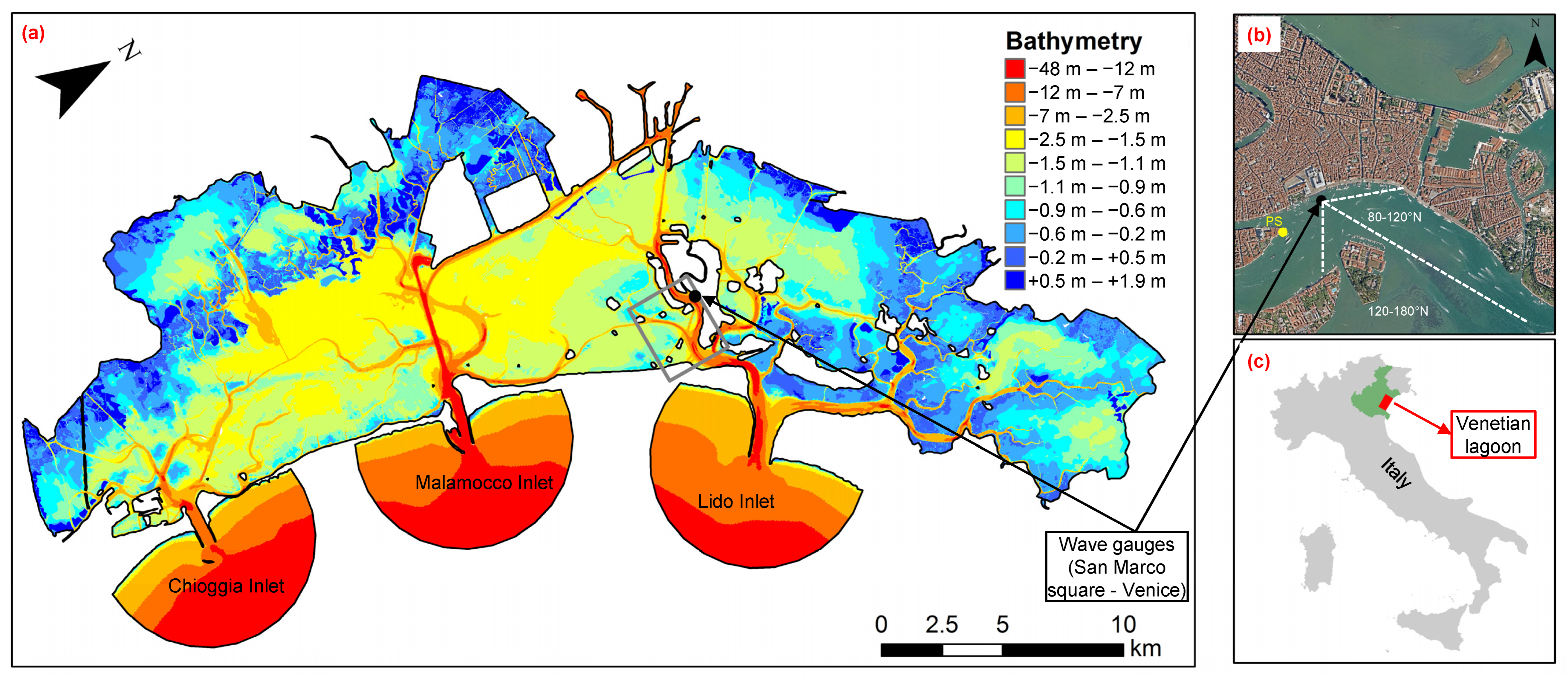
Figure 1a shows the bathymetry of the lagoon based on a mosaic of topographic data recorded in different years (http://cigno.ve.ismar.cnr.it, accessed on 1 May 2022). Almost all the areas coloured in blue correspond to salt marshes that developed between 0.25 m and 0.37 m above average sea level (Ivajnšič et al. [25]). Venice is located in the northern part, next to the Lido inlet.
High water levels (Acqua Alta events) in the Venetian lagoon develop due to a combination of astronomical tides and meteorological storm surges (Umgiesser et al. [26]). The semidiurnal tidal range is on average 0.55 m and up to 1 m in spring conditions (Helsby [27]), one of the highest observed in the Mediterranean. High storm surges are generated by low-pressure systems and winds blowing from the northeast and southeast, named Bora and Scirocco (Ruol et al. [28]). Especially, this latter long-fetch wind that blows over the whole Adriatic Sea is responsible for the pilling up of the water in the northern Adriatic Sea (Trincardi et al. [5]) and therefore, together with tides, the effects of subsidence and sea level rise, causing the flooding of Venice. The highest events occurred on 4 November 1966 (Canestrelli et al. [29]) when the sea level rose approximately 1.94 m above ZMPS (Italian acronym for Zero Mareografico Punta della Salute, the local tidal datum). Recently, the second-highest event was measured, on 12 November 2019 at 22.50 UTC, during which the water level reached 1.87 m ZMPS (Cavaleri et al. [30]).
The Mo.S.E. system was designed to mitigate the effect of the high tide conditions and reduce flooding events (for technical details, see [31] and https://www.mosevenezia.eu/progetto/, accessed on 15 May 2022). The system consists of 78 independently oscillating mobile barriers that can temporarily close the lagoon inlets and maintain the water level in front of San Marco square (Venice) below a certain threshold (1.10 m ZMPS in extreme cases, more frequently in the range of 0.7 m–0.9 m ZMPS). The Mo.S.E. is not intended to protect specifically San Marco square, which has elevations below these thresholds, i.e., mean elevation of the square is ~0.95 m ZMPS, with some areas in front of San Marco church lower than 0.7 m ZMPS (Favaretto et al. [32]). Therefore, the basin in front of the square represents an interesting location to measure the waves generated by winds blowing from the southeast (see fetch sectors in Figure 1b). In fact, during extreme events, the flooding of the square is mainly caused by the backflow through the drainage system but could also be exacerbated by wave overtopping (Ruol et al. [33]).
The first Mo.S.E. closures were in October 2020 and so far, the lagoon was closed during more than 35 events when the expected water levels were forecast to be higher than 1.10 m ZMPS (1.30 m during the very first closures) in front of Venice. A full description of the first closures is reported in Mel et al. [34].
The tidal and wind data used in the present study come from the “Centro Previsioni e Segnalazioni Maree” (CPSM) and the “Istituto superiore per la protezione e la ricerca ambientale” (ISPRA) databases, stored with a time step of 10 min. As generally used in this area, the local tidal datum is the official reference of Punta della Salute gauge (named as mentioned before ZMPS ~ +0.23 m below the Italian national datum), located in front of San Marco square (Figure 1b).
2.2. In Situ Wave Measurements
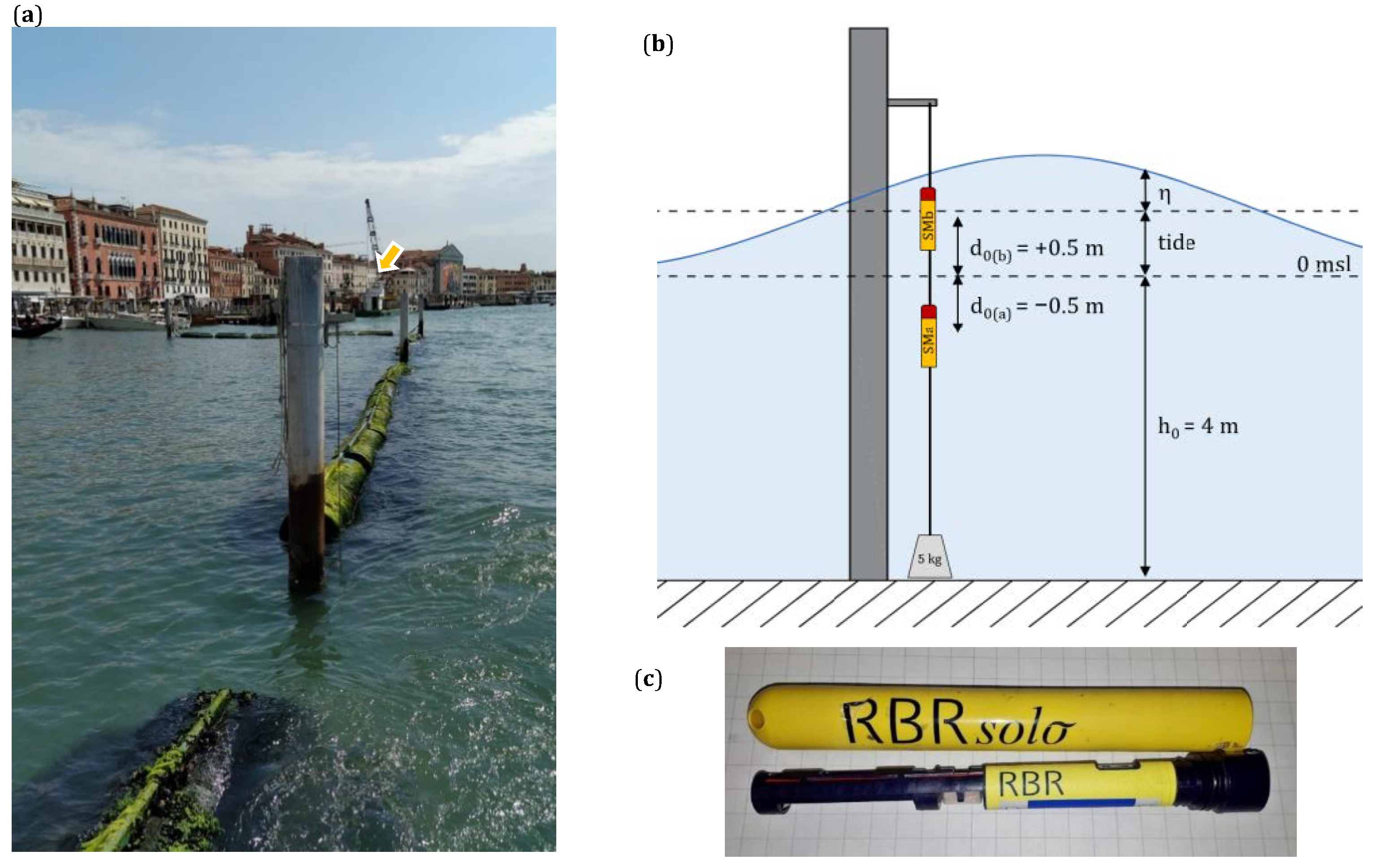
Two small pressure gauges (RBR Solo D wave), named “SMa” and “SMb”, were installed in a retaining pile in front of San Marco square in Venice (IT), Lat. 45°25′58.49″ N and Lon. 12°20′26.50″ E, for the period 16 July 2020–31 December 2021. The recording frequency is 16 Hz, allowing for continuously acquiring the surface elevations. Figure 2 shows the deployed instruments, the retaining pile where the gauges were hung up and a scheme of the installation. The instruments were attached to a steel cable with a 5 kg ballast. The water depth in correspondence of the pile is about 4 m. The surveys for instrument maintenance and data download occurred approximately monthly.
Pressure transducers are instruments commonly used for wave measurements (Karimpoura and Chen [35]) and, following the linear wave theory, the recorded data contain three signals: an atmospheric pressure, an hydrostatic pressure and a dynamic pressure (Equation (1)).
where ρ is the water density; k the wave number; d0 is the gauge submergence with respect to the mean sea level; d(t) is the instantaneous submergence (=d0 + tide); h0 is the water depth with respect to the msl, h(t) is the instantaneous water depth (h0 + tide) and η(t) is the surface elevation.
In Equation (1), the second signal represents the sensor’s depth used to define the water depth in time h(t). The third signal is a result of the wave motion and is used to estimate wave properties. Since the dynamic pressure can be attenuated markedly with the frequency and the depth of the transducer (Cavaleri et al. [36]), the gauge must always be submerged but, at the same time, the submergence must not be such as to filter the shortest frequencies, i.e., those of the waves generated by winds or by small boats. The gauges were therefore installed with two different submergences (d0) to measure waves both in low and high tide conditions. The “SMa” gauge was placed at −0.5 m msl and the “SMb” at +0.5 m msl (Figure 2b). This latter gauge is essentially used to check the accuracy of the wave signal correction hereafter described.
The dynamic pressure signal measured with a pressure gauge cannot be used directly for wave analysis, and requires the proper correction and preparation; otherwise, it leads to an underestimation of the wave height. The pressure data correction for dynamic pressure attenuation in depth was performed in time domain and no additional frequency spectrum correction has been applied since it is not essential in shallow depths. The first operation consists of removing the atmospheric pressure and the tide from the gauge signal to obtain the dynamic pressure. To account for the dynamic pressure loss at the sensor depth, this latter series is split into portions of 10 min and the actual d(t) and h(t) are calculated by averaging the data over each section allowing the evaluation of the depth-corrected η(t) signal. Finally, η(t) is analysed to compute the typical spectral and statistical wave parameters every 30 min: spectral, significant and maximum wave heights (Hm0, HS and Hmax); mean and peak wave periods (Tm and Tp).
2.3. Numerical Wave Modelling
The SWAN (Simulating WAves Nearshore) model (version 41.31) is used to simulate the wind-generated waves in the Venetian lagoon. The model, developed by the Delft University of Technology (Booij et al. [37,38]), solves the wave action balance equation accounting for several physics, sinks and sources, such as the generation by wind. This mechanism is critical for the specific case of enclosed basins, such as lagoons and lakes since the wind-wave growth starts from land and the wave boundary condition is null (Favaretto et al. [39]). The model solves the equations with a finite difference approach using an implicit iterative direct method for time integration (Sartini et al. [40]).
For the present analysis, the SWAN model is run with the third-generation option (GEN3) in stationary mode. The steady-state assumption means that the winds remain steady sufficiently long enough for the waves to attain fetch-limited conditions. This assumption is reliable for the Venetian lagoon since the maximum fetch in front of an Marco square is limited to 3 km, and fetch-limited conditions are reached after only ~10–15 min. As a consequence, the steady state assumption does not consider the change of water levels within the simulation. This is, however, acceptable for the Venetian lagoon where the characteristic time for water level variations and for wave generation and propagation are slightly different: in hours for the first phenomenon and minutes for the second. The change of water levels can therefore be considered negligible for wave modelling in this specific enclosed basin.
The numerical properties are set to the default values, using the NUMerics STOPC command (dabs = 0.005, drel = 0.01, curvat = 0.005, npnts = 99.5) with a limiter parameter equal to 0.1. The threshold depth depmin is set equal to 0.05 m. The formulation for depth-induced wave breaking is the default Battjes and Janssen [41] (BREA command with alpha = 1 and gamma = 0.73). The bottom friction is activated with the FRIC JON command that considers a semi-empirical expression (Hasselmann et al. [42]) with a constant friction coefficient equal to 0.038 m2s−3. The KOMEN package [43] is used for wind input, quadruplet interactions and whitecapping (Christakos et al. [14] and Aydoğan and Ayat [16]). The wind velocity used by SWAN is the wind velocity at 10 m elevation (U10), which is then converted into calculations of the friction velocity u*, defined as u*2 = CD U102, where CD is the wind-drag coefficient. In the following simulations, the second-order polynomial formula proposed by Zijlema et al. [44] for CD is used. Since the wind measurements used to force the model are available at 12.5 m elevation, a correction (=0.93) based on the wind logarithmic profile is applied to the wind intensity.
The simulations are performed by setting a uniform water level, a uniform wind field and a null wave spectrum at the upwind boundary, in order to evaluate only the waves generated by the wind blowing over the enclosed basin. An additional corrective coefficient for wind velocity is introduced to account for slightly non-homogenous wind fields in the lagoon. The total correction coefficient applied to U10 is equal to 0.75. Three north-oriented, structured and regular grids are used. The first and the second cover the entire lagoon with open and closed inlets, respectively, and a resolution of 100 m (154,164 elements). The latter is a nested grid located in front of San Marco square (grey box in Figure 1) with a resolution of 10 m (94,581 elements). The wave boundary conditions applied to the nested grid are based on the result obtained from the main ones.
The directional grid range from 0° to 360° N with 72 bins (interval = 5° N). The frequency grid is set between 0.05 Hz and 2 Hz, considering 36 logarithmically spaced bins. The choice of the proper frequency range is crucial since it should be a compromise between accuracy and computational load. It must cover the range of expected wave frequencies generated by the winds and an unsuited choice of frequency range and discretization lead to noteworthy results. For the case of enclosed basins, the lower value (0.05 Hz) has little influence on the final results since it only increases the discretization in a range where no waves are expected (i.e., wave periods larger than 6 s). For instance, considering a lower limit equal to 0.15 Hz, for the investigated lagoon, the differences in terms of HS are of the order of 2% with respect to the limit of 0.05 Hz. On the contrary, the upper value requires specific attention. Bottema et al. [45] suggested that the upper value of 2 Hz is necessary to properly resolve the spectrum and for hindcasting/forecasting waves in enclosed basins.
3. Results
3.1. Measured and Computed Wind Waves
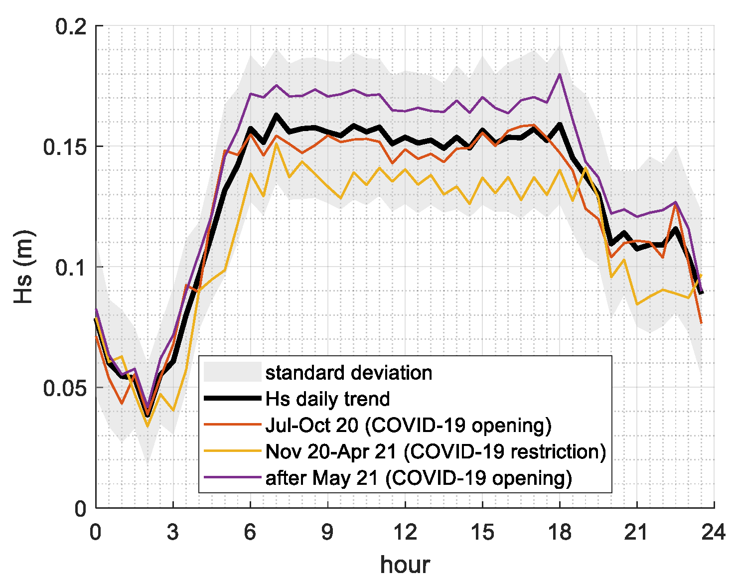
The recorded wave series is the result of both boat traffic waves and wind waves. Whereas wind waves occur occasionally, traffic waves can be considered as a frequent hydrodynamic forcing in the investigated area. In fact, the series shows a daily trend caused by boat traffic in the San Marco basin. The black line in Figure 3 is the daily trend computed as the average of the recorded HS relative to each hour for the entire time series. The waves between 6 am and 6 pm are characterized by a mean HS of about 15 cm and, during the night, the waves decrease and the minimum is expected at 2 am with mean HS less than 5 cm.
The start of the wave measurements (16 July 2020) took place a few months after the start of the COVID-19 pandemic, which largely changed human habits and life. Therefore, the observed wave time series is affected by a trend triggered by the Italian measures adopted during the pandemic. This trend is a consequence of different boat traffic in the Venetian lagoon that does not obviously affect the wind-generated waves, i.e., the focus of the present investigation. For clarity and completeness, a short discussion of the pandemic’s effect on the magnitude of the waves is hereafter described.
Several restrictive measures were applied in Italy to oppose the COVID-19 disease, followed by opening measures to restart the activities [46,47]. Braga et al. [48] found that from March to April 2020, i.e., during the first lockdown, the mean HS decrease by about 50% since local water traffic was dramatically reduced. As a consequence, unprecedented water transparency was reported in the city canals, leading to several positive environmental consequences.
In the period from July–October 2020, a series of measures allowed for the restart of activities after the first national lockdown; in the period from November 2020–April 2021, a Prime Ministerial Decree (DPCM) introduced again restrictive measures to reduce the pandemic spreading. From May 2021 until now, the decrees have also allowed a gradual reopening based on the administration of vaccines against COVID-19. Figure 3 shows the daily trend computed for these three periods, where the effect of the restrictive and opening measure on the boat traffic is detectable.
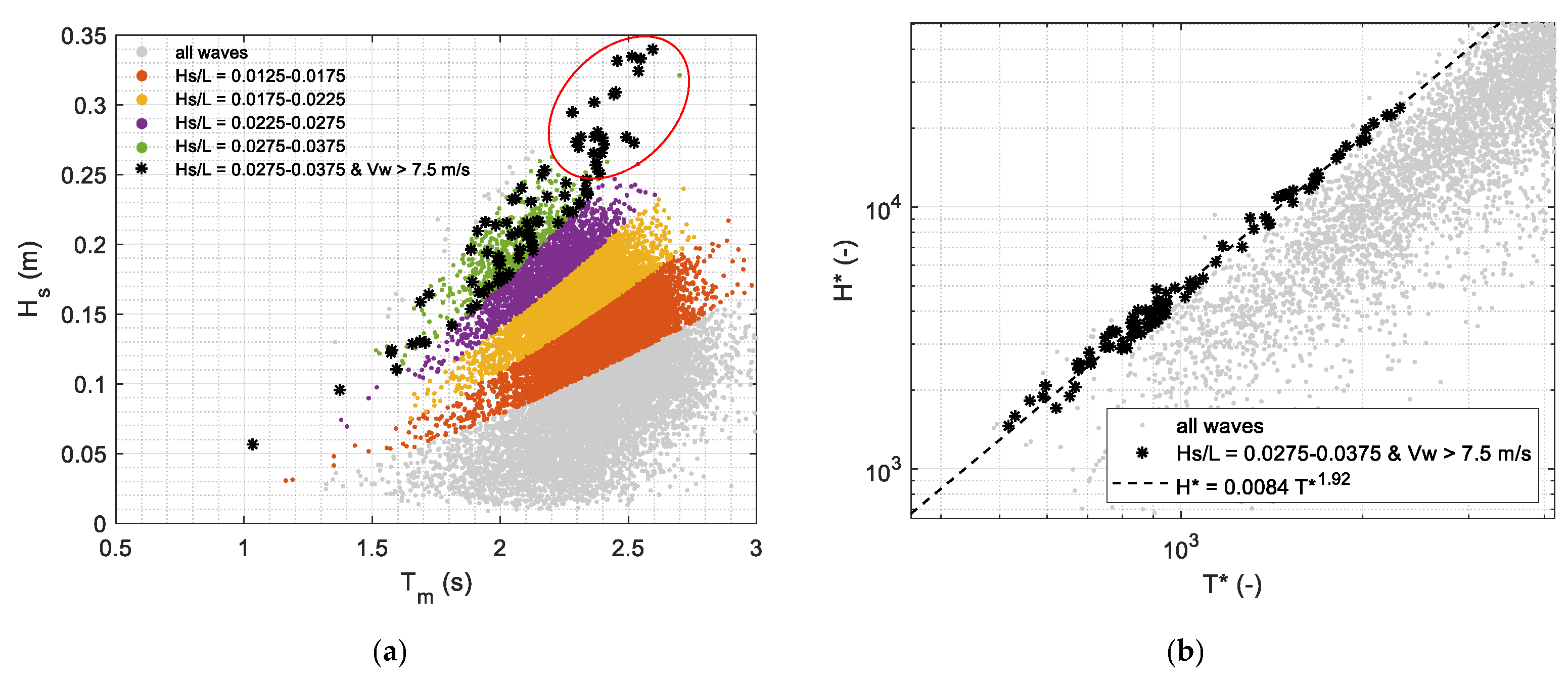
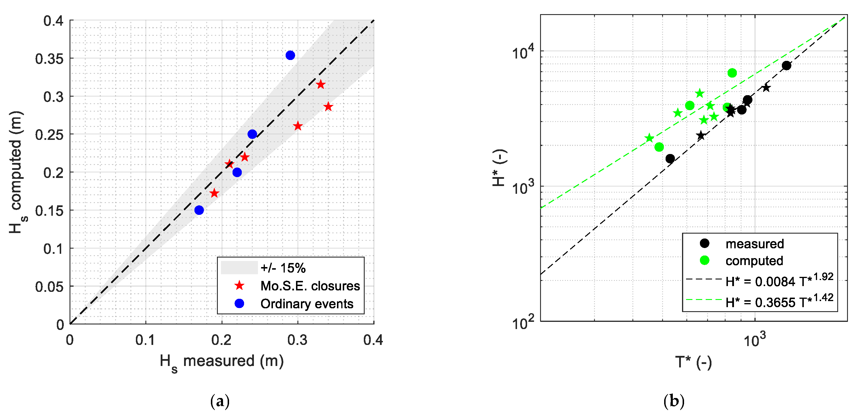
Due to their specific generation, boat and wind waves have considerably different characteristics, e.g., wave form, period and length (Hofmann et al. [49]). In particular, the relationship between the wave height and the wave period vary according to the wave steepness (ratio between the significant wave height and the wave length HS/L), and can be used to highlight, together with the simultaneous wind velocity Vw, the wave generated by different forcing. In Figure 4a, HS are plotted against the corresponding mean wave periods and four subsets of them are highlighted based on their wave steepness. The set of waves with HS/L in the range 0.025–0.035, also associated with wind velocity Vw larger than 7.5 m/s (black stars in the figure), includes all the waves corresponding to the highest HS (larger than 0.25 m, points inside the red ellipse in the figure), which are reasonably those generated by stormy events. Figure 4b shows the same points but plotted in terms of dimensionless significant wave height H* and dimensionless wave period T*. In fact, as pointed out by Toba [50], there is a simple similarity in wind waves between H* = g HS/u*2 and T* = gTm/u*, where u* = CD Vw is the wind stress (CD is the friction coefficient based on Zijlema et al. [44] formula). These dimensionless variables could therefore be used to look for physical dependencies and derive power-law fits. The dependency law between H* and T* for this subset of waves is H* = 0.0084 T* 1.92. It is important to recall that the investigated area is a rather small, enclosed basin where wind waves are relative to a young sea growth since the wave generation is only forced by winds blowing over the lagoon. In fact, the exponent of the power-law dependency between H* and T* is higher than 5/3, as in the reference case for young waves shown by Badulin and Grigorieva [51] and by Gagnaire-Renou et al. [52].
The maxima HS recorded by the wave gauges are selected during some Mo.S.E. closures or during some ordinary wind events. The selection of the storms is based on two criteria: (i) maximum wind velocity Vw larger than 10 m/s (i.e., ~ the 95th percentile); and (ii) maximum wave height HS during the wind storm larger than 0.15 m. It is important to point out that the San Marco basin is exposed only to winds blowing from 80°–180° N since it is sheltered from other wind directions (Figure 1b). Consequently, only ten recorded stormy events (six during Mo.S.E. closures and four during ordinary events) force the generation of wind waves in front of San Marco square in the observed period. The list of events is reported in Table 1, which summarizes all the main information: HS, Tm, sea levels (z) at the Punta della Salute gauge and at the Lido inlet, wind intensity (Vw) and wind direction (Dw). The HS ranges between 0.17 and 0.34 m, and the corresponding Vw ranges between 10.6 and 22.2 m/s. The longest lagoon closure, lasting more than 40 h, was during event no. 3. With the exception of event no. 7, all the selected events are relative to the directional sector located between 120° N and 180° N. This sector corresponds to Scirocco winds responsible for Acqua Alta events when the Mo.S.E. system operates more frequently. The direction that characterizes event no. 7 usually does not cause high water levels in the northern and central basins of the Venetian lagoon. However, it is interesting to also analyze this condition, during which time the Mo.S.E. was not closed but strong winds blew, generating high waves in the San Marco basin.
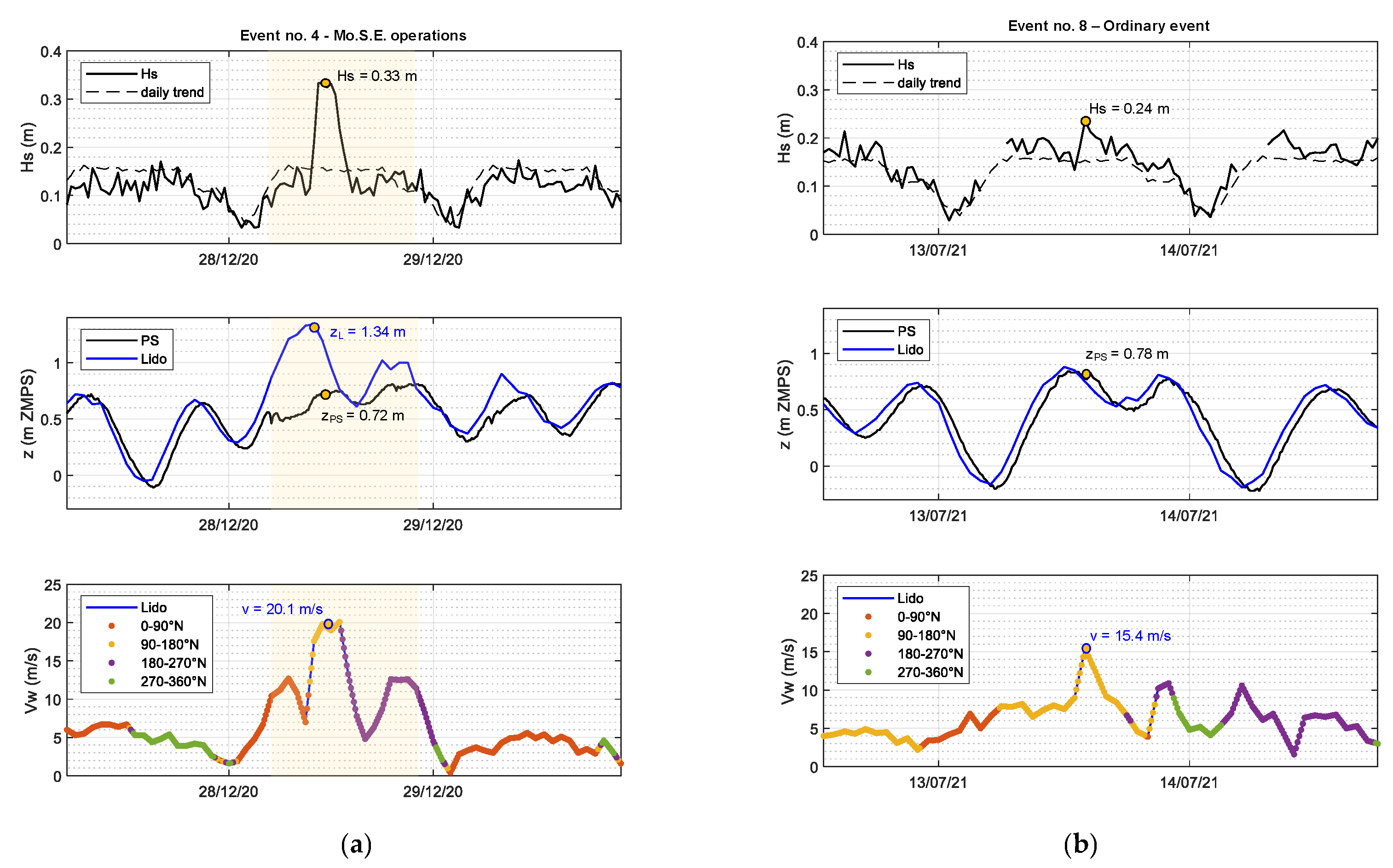
Figure 5 shows the time series of HS, z, Vw and Dw during a Mo.S.E. closure (28 December 2020, event no. 4) and an ordinary event (13 July 2021, event no. 8). In the figures, the HS daily trend (previously shown in Figure 3) is also plotted to enhance the wave resulting from the storms. These two storms were selected in order to compare events when the water level inside the lagoon was similar (0.72 m and 0.78 m respectively).
During event no. 4, the lagoon was closed for approximately 17 h, and the water levels reached 1.34 m at the inlets and remain below 0.8 m at the Punta della Salute tidal gauge during the whole closure. The event was characterized by winds up to 20.1 m/s blowing from 168° N that generated waves with HS up to 0.33 m in front of San Marco square. The HS during the ordinary event no. 8 was smaller compared to event no. 4, with maximum Hs equal to 0.24 m. The water level was 0.78 m at the Punta della Salute and the wind was equal to 15.4 m/s blowing from 130° N. Both the events are useful to highlight that the wave generation is almost simultaneous to the maximum wind intensity, confirming the fetch limited hypothesis and allowing steady-state simulations. The same figures are presented in the Supplementary Materials for all the other events.
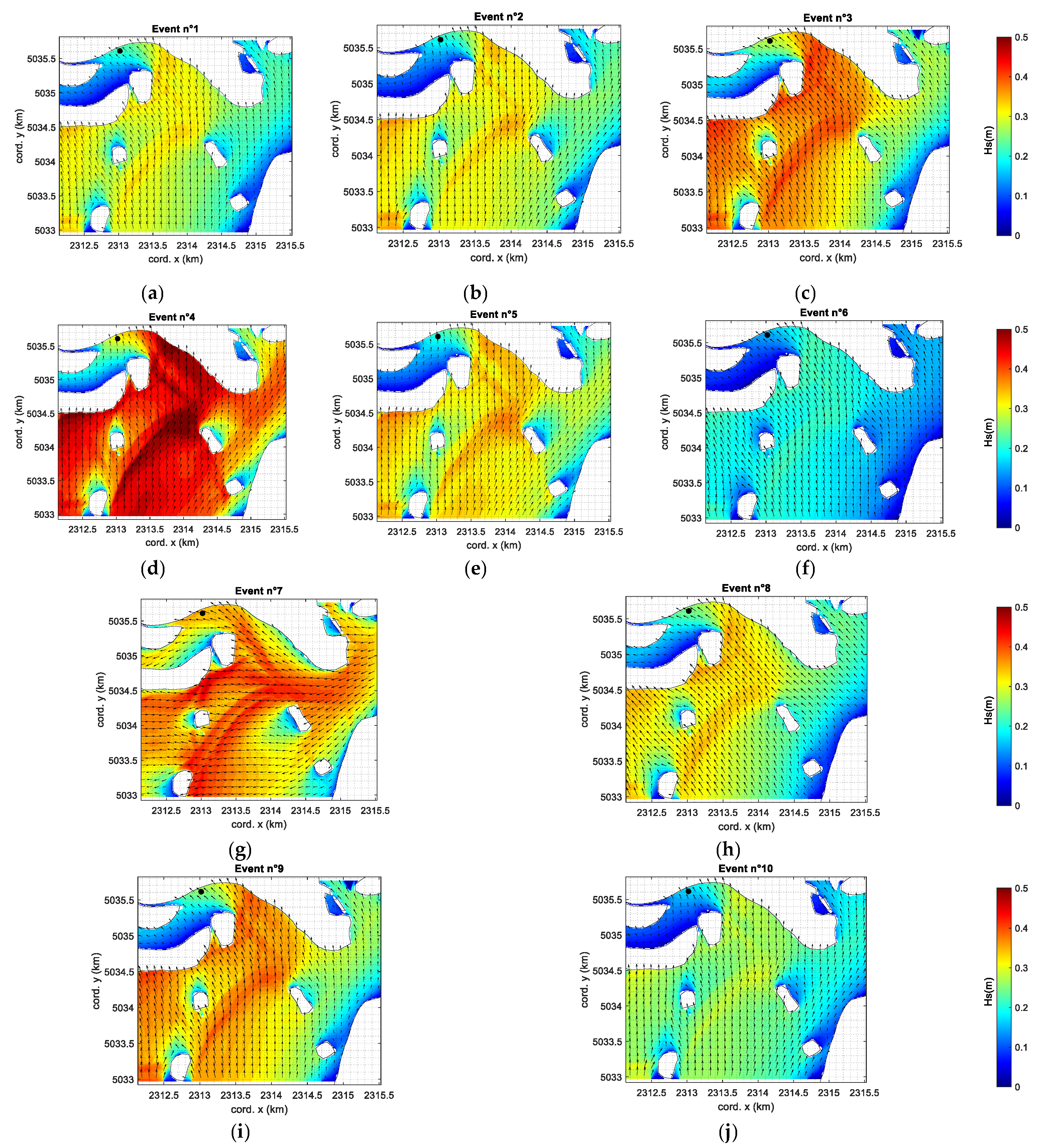
The ten events are simulated with the SWAN model, using the settings reported in Section 2.3. The wind fields used are uniform and the wind intensities and directions for each storm are the ones listed in Table 1, which are based on wind measurements. The nested grid model results in terms of HS are shown in Figure 6 for all the events; the black arrows indicate the wave directions and their lengths are proportional to HS. For completeness, the HS results mapped for the whole lagoon (main model grid) are presented in the Supplementary Materials. Among all the events, only event no. 7 is a typical Bora storm with winds blowing from the north-east/east and the San Marco basin is partially shadowed from this direction. However, due to diffraction, the waves enter inside the basin and reach approximately 35 cm in front of San Marco square. The other events are typical Scirocco storms during which high storm surges are generated by the wind blowing on the whole Adriatic Sea and, in fact, when the Mo.S.E. operates more frequently. The wave height is high (up to 50 cm) in the most exposed part of the San Marco basin, i.e., east of San Marco square.
Figure 7a shows the comparison between the measured and the computed significant wave height HS: the six events during Mo.S.E. closures are plotted in red, and the others in blue (four ordinary events). In general, the comparisons show a fairly good agreement between measured and predicted Hs values. To quantitatively assess the quality of the estimates, three performance metrics were calculated: the coefficient of efficiency NSE Nash et al. [53], the index of agreement D Willmott et al. [54] and the square of the correlation coefficient r2. Complete disagreement is described by negative NSE, D = 0 and r2 = 0 and. All indexed are = 1 for perfect agreement. For significant wave heights, NSE is equal to 0.6761, D is equal to 0.9205 and r2 is equal to 0.6869.
Figure 7b shows the relationship between H* and T* for both measured and computed waves. In the enclosed basins, the prediction of the wave period is not straightforward and is strictly related to the wind input source term. The two dependency laws shown in the figure are slightly different but the results for the wave period are reasonable considering that this parameter has a larger variability (Vieira et al. [55]).
3.2. Effect of Mo.S.E. Closures on Wind Waves
The validation presented in the previous paragraph allows for broadening the numerical results to the whole lagoon in order to better understand the effects of the closure of the inlets on the wind-wave propagation. The six events during Mo.S.E. closures (events no. 1, 3, 4, 5, 9 and 10) are re-simulated considering the inlets opened and therefore setting the sea level inside the lagoon as the maximum value recorded at the Lido inlet. In detail, the water levels (z) for the six events are:
- Event no. 1 closed scenario z = 0.69 m, open scenario z = 1.19 m (z decrease ~ 42%);
- Event no. 3, closed scenario z = 0.83 m, open scenario z = 1.28 m (z decrease ~ 35%);
- Event no. 4, closed scenario z = 0.72 m, open scenario z = 1.34 m (z decrease ~ 46%);
- Event no. 5, closed scenario z = 0.56 m, open scenario z = 1.07 m (z decrease ~ 47%);
- Event no. 9, closed scenario z = 0.81 m, open scenario z = 1.38 m (z decrease ~ 41%);
- Event no. 10, closed scenario z = 0.58 m, open scenario z = 1.05 m (z decrease ~ 45%).
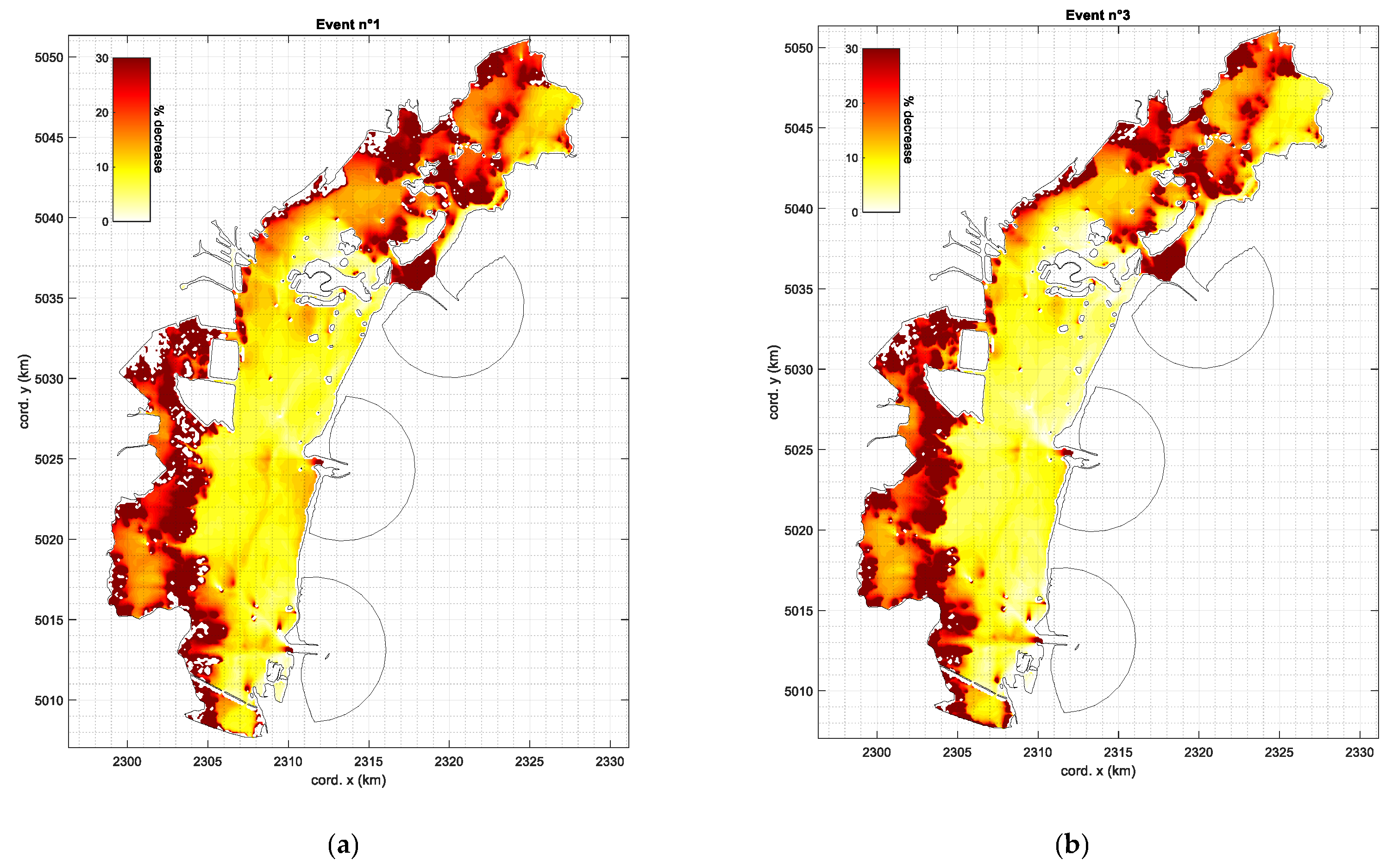
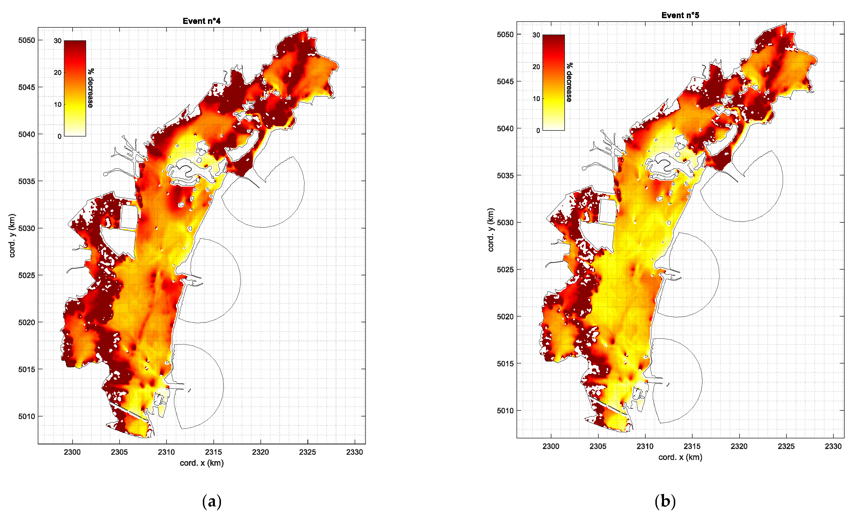
Obviously, the Hs is lower during the Mo.S.E. closures due to the lower water levels. The Hs decrease with respect to the conditions with open inlets and is not uniform within the lagoon. Figure 8, Figure 9 and Figure 10 show the percentage decrease between the modelled Hs in the closed and opened Mo.S.E. gates for the six events. The results relative to event no. 4 show the largest differences between the two scenarios (with closed Mo.S.E. −25% on average in the whole lagoon). In general, the decrease is very high in all the areas that, during the Mo.S.E. closures, were emerged or little submerged.
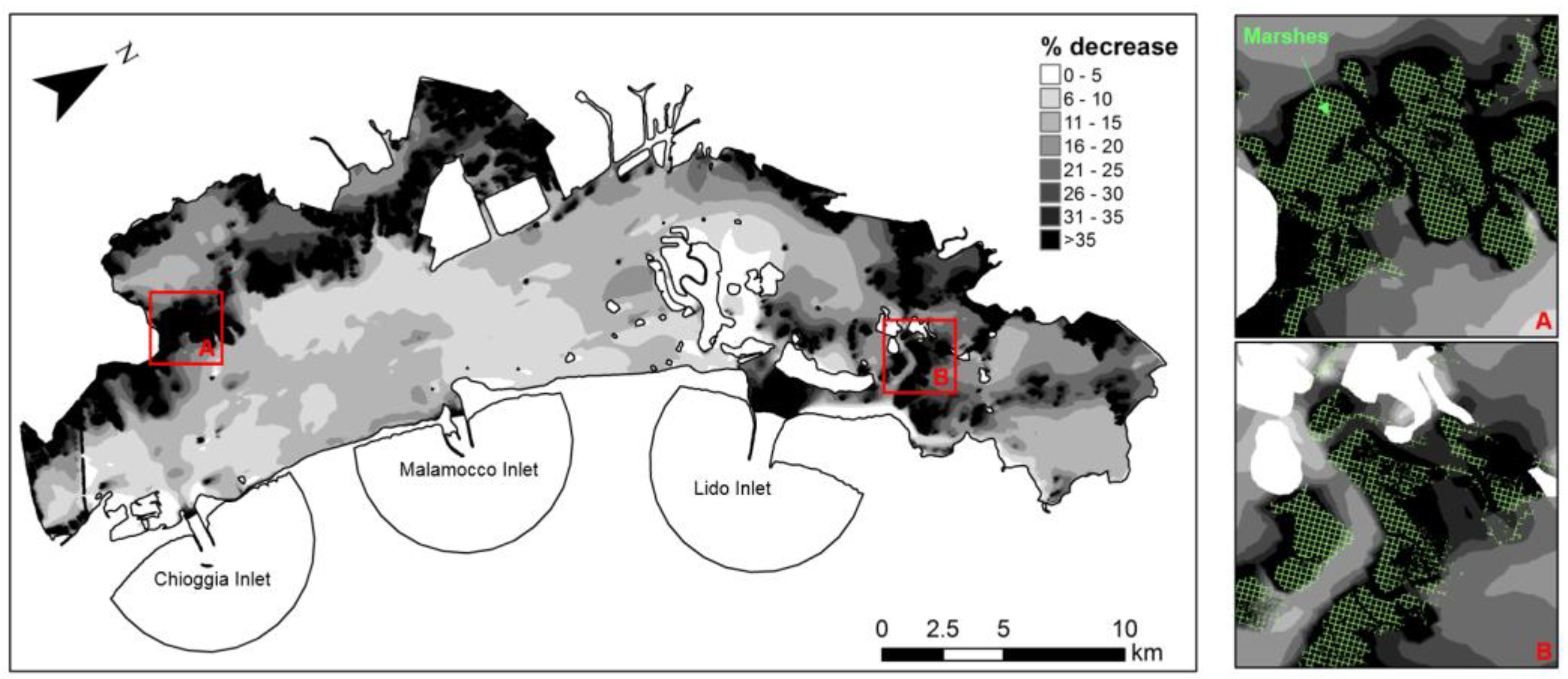
To further investigate the effect of the Mo.S.E. closures, the difference in terms of HS obtained for the six events is averaged and shown in Figure 11. For the six events, the average decrease in terms of water levels between the closed and opened scenario is approximately 43%. The average Hs decrease in the whole lagoon is approximately 22%, and the figure is useful to highlight the areas where the decrease of Hs due to lower water levels is larger. As aforementioned, the areas with the largest predicted differences are the shallow tidal flats and salt marshes located in the south-western and northern parts (black zones in the main figure, green areas in the two zooms). In these areas characterized by mean water depths in the range 0.25–0.37 m, the decrease is on average 48% during the Mo.S.E closures, whereas in the remaining deeper areas, the decrease is on average 19%. In the San Marco basin, the decrease ranges between 1 and 8%.
The Mo.S.E. closures have therefore a non-negligible effect on the wind-wave propagation. On one hand, from an engineering perspective, smaller waves reduce the risk of flooding due to wave overtopping in the city of Venice [33] and ease the loads applied to the maritime structures (i.e., floating breakwaters). On the other hand, modification of the wave height and energy could considerably change the sediment mechanism inside the lagoon with impacts on the lagoon morphodynamics. For instance, since the marshes flooding decreases during the floodgate closure, the sedimentation induced by the combined effect of lower water levels and lower wind waves changes, influencing the sustainability of these tidal landforms (Tognin et al. [56]).
4. Conclusions
The present study investigated the effect of the Mo.S.E. closures on the wind-wave generation in front of the San Marco basin and, as a result, in the whole Venetian lagoon through a combined experimental and numerical analysis. Two pressure wave gauges were installed in front of the San Marco square from July 2020 to December 2021 and ten stormy events were selected (during Mo.S.E. closures and ordinary events) and simulated with the SWAN spectral wave model. The peculiarity of this combined analysis is two-fold. Firstly, wave measurements in the Venetian lagoon are sparse and fragmented and the in situ investigation allowed for establishing a unique and valuable dataset. Secondly, the validations of wave models in enclosed basins, such as lagoons, are rare due to both the lack of data and the critical issue associated with the wind-wave generation, i.e., the wind-wave growth starts from land and the wave boundary condition is null.
It is worthy to highlight that the start of the measurements took place a few months after the start of the COVID-19 pandemic and the measured average significant wave height HS time series influenced by boat traffic shows a fluctuating trend (in the range of −8% to +14%) associated with the Italian measures adopted to combat the pandemic.
The combined analysis allowed for comparing the modelled wind-wave propagation during flood-regulated conditions (Mo.S.E. closures) and non-regulated events. During the Mo.S.E. closures, due to the lower water level (on average 43% of water level reduction), the differences in terms of Hs are of the order of 22% but with areas that experienced higher decreases. The largest differences (−48%) were predicted as expected in the shallow tidal flats and salt marshes located in the south-western and northern parts of the lagoon.
The temporary closure of the Venetian lagoon aimed at preventing flooding has, therefore, an impact on the wind-wave propagation with positive and negative consequences. From an engineering perspective, lower waves induce smaller overtopping discharge over the quays of Venice and reduce the loads applied to the maritime structures. From an environmental perspective, the decrease in the waves could also considerably change the lagoon’s hydrodynamics and morphodynamics, with effects on the morphological variations.
Future research work should carry out in situ observations acquired at several locations across the Venetian Lagoon in order to extend the wave dataset and numerical validation, and further investigate both the boat waves and the effects of the storm-surge barriers on wind-wave propagation inside this fragile environment.
Supplementary Materials
The following supporting information can be downloaded at: https://www.mdpi.com/article/10.3390/w14162579/s1: Figures S1–S5 show the time series of HS, z, Vw and Dw during the ten analyzed events. Figures S6–S15 show the HS numerical results mapped for the whole Venetian lagoon for the ten analyzed events.
Author Contributions
Conceptualization, C.F.; methodology, C.F., G.M., M.V. and G.M.S.; investigation, C.F. and M.V.; data curation, G.M. and G.M.S.; writing—original draft preparation, C.F.; writing—review and editing, C.F., G.M., M.V. and G.M.S.; supervision, C.F. All authors have read and agreed to the published version of the manuscript.
Funding
This research received no external funding.
Acknowledgments
We are grateful to Piero Ruol and Luca Martinelli (University of Padova) for the fruitful discussions.
Conflicts of Interest
The authors declare no conflict of interest.
References
- Fletcher, C.A.; Spencer, T. Flooding and Environmental Challenges for Venice and Its Lagoon: State of Knowledge; Cambridge University Press: Cambridge, UK, 2005; ISBN 978-0-521-84046-0. [Google Scholar]
- Defendi, V.; Kovačević, V.; Arena, F.; Zaggia, L. Estimating sediment transport from acoustic measurements in the Venice Lagoon inlets. Cont. Shelf Res. 2010, 30, 883–893. [Google Scholar] [CrossRef]
- Ghinassi, M.; Brivio, L.; D'Alpaos, A.; Finotello, A.; Carniello, L.; Marani, M.; Cantelli, A. Morphodynamic evolution and sedimentology of a microtidal meander bend of the Venice Lagoon (Italy). Mar. Pet. Geol. 2018, 96, 391–404. [Google Scholar] [CrossRef]
- Scarpa, G.M.; Zaggia, L.; Manfè, G.; Lorenzetti, G.; Parnell, K.; Soomere, T.; Rapaglia, J.; Molinaroli, E. The effects of ship wakes in the Venice Lagoon and implications for the sustainability of shipping in coastal waters. Sci. Rep. 2019, 9, 1–14. [Google Scholar] [CrossRef] [PubMed] [Green Version]
- Trincardi, F.; Barbanti, A.; Bastianini, M.; Benetazzo, A.; Cavaleri, L.; Chiggiato, J.; Papa, A.; Pomaro, A.; Sclavo, M.; Tosi, L.; et al. The 1966 flooding of Venice: What time taught us for the future. Oceanography 2016, 29, 178–186. [Google Scholar] [CrossRef] [Green Version]
- Trigo, I.F.; Davies, T.D. Meteorological conditions associated with sea surges in Venice: A 40 year climatology. Int. J. Climatol. J. R. Meteorol. Soc. 2002, 22, 787–803. [Google Scholar] [CrossRef]
- Lionello, P.; Nicholls, R.J.; Umgiesser, G.; Zanchettin, D. Venice Flooding and Sea Level: Past Evolution, Present Issues, and Future Projections (Introduction to the Special Issue). Nat. Hazards Earth Syst. Sci. 2021, 21, 2633–2641. [Google Scholar] [CrossRef]
- Zanchettin, D.; Bruni, S.; Raicich, F.; Lionello, P.; Adloff, F.; Androsov, A.; Antonioli, F.; Artale, V.; Carminati, E.; Ferrarin, C.; et al. Sea-level rise in Venice: Historic and future trends. Nat. Hazards Earth Syst. Sci. 2021, 21, 2643–2678. [Google Scholar] [CrossRef]
- Umgiesser, G. The impact of operating the mobile barriers in Venice (MOSE) under climate change. J. Nat. Conserv. 2020, 54, 125783. [Google Scholar] [CrossRef]
- Mel, R.; Carniello, L.; D'Alpaos, L. Addressing the effect of the Mo. SE barriers closure on wind setup within the Venice lagoon. Estuar. Coast. Shelf Sci. 2019, 225, 106249. [Google Scholar] [CrossRef]
- Tognin, D.; Finotello, A.; D’Alpaos, A.; Viero, D.P.; Pivato, M.; Mel, R.A.; Defina, A.; Bertuzzo, E.; Marani, M.; Carniello, L. Loss of geomorphic diversity in shallow tidal embayments promoted by storm-surge barriers. Sci. Adv. 2022, 8, eabm8446. [Google Scholar] [CrossRef]
- Tommasini, L.; Carniello, L.; Ghinassi, M.; Roner, M.; D'Alpaos, A. Changes in the wind-wave field and related salt-marsh lateral erosion: Inferences from the evolution of the Venice Lagoon in the last four centuries. Earth Surf. Process. Landf. 2019, 44, 1633–1646. [Google Scholar] [CrossRef]
- Carniello, L.; D’Alpaos, A.; Defina, A. Modeling wind waves and tidal flows in shallow micro-tidal basins. Estuar. Coast. Shelf Sci. 2011, 92, 263–276. [Google Scholar] [CrossRef]
- Christakos, K.; Björkqvist, J.V.; Tuomi, L.; Furevik, B.R.; Breivik, Ø. Modelling wave growth in narrow fetch geometries: The white-capping and wind input formulations. Ocean. Model. 2021, 157, 101730. [Google Scholar] [CrossRef]
- Moeini, M.H.; Etemad-Shahidi, A. Application of two numerical models for wave hindcasting in Lake Erie. Appl. Ocean. Res. 2007, 29, 137–145. [Google Scholar] [CrossRef]
- Aydoğan, B.; Ayat, B. Performance evaluation of SWAN ST6 physics forced by ERA5 wind fields for wave prediction in an enclosed basin. Ocean. Eng. 2021, 240, 109936. [Google Scholar] [CrossRef]
- Scarton, F. Long-term trend of the waterbird community breeding in a heavily man-modified coastal lagoon: The case of the Important Bird Area “Lagoon of Venice”. J. Coast. Conserv. 2017, 21, 35–45. [Google Scholar] [CrossRef]
- Molinaroli, E.; Guerzoni, S.; Sarretta, A.; Masiol, M.; Pistolato, M. Thirty-year changes (1970 to 2000) in bathymetry and sediment texture recorded in the Lagoon of Venice sub-basins, Italy. Mar. Geol. 2009, 258, 115–125. [Google Scholar] [CrossRef] [Green Version]
- Sarretta, A.; Pillon, S.; Molinaroli, E.; Guerzoni, S.; Fontolan, G. Sediment budget in the Lagoon of Venice, Italy. Cont. Shelf Res. 2010, 30, 934–949. [Google Scholar] [CrossRef] [Green Version]
- Ferrarin, C.; Cucco, A.; Umgiesser, G.; Bellafiore, D.; Amos, C.L. Modelling fluxes of water and sediment between Venice Lagoon and the sea. Cont. Shelf Res. 2010, 30, 904–914. [Google Scholar] [CrossRef] [Green Version]
- Bellafiore, D.; Umgiesser, G.; Cucco, A. Modeling the water exchanges between the Venice Lagoon and the Adriatic Sea. Ocean. Dyn. 2008, 58, 397–413. [Google Scholar] [CrossRef]
- Tambroni, N.; Seminara, G. Are inlets responsible for the morphological degradation of Venice Lagoon? J. Geophys. Res. Earth Surf. 2006, F03013, 111. [Google Scholar] [CrossRef] [Green Version]
- Scarpa, G.M.; Braga, F.; Manfè, G.; Lorenzetti, G.; Zaggia, L. Towards an Integrated Observational System to Investigate Sediment Transport in the Tidal Inlets of the Lagoon of Venice. Remote Sens. 2022, 14, 3371. [Google Scholar] [CrossRef]
- Ackroyd, P. Venice: Pure City; Nan, A.T., Ed.; Doubleday: New York, NY, USA, 2009. [Google Scholar]
- Ivajnšič, D.; Kaligarič, M.; Fantinato, E.; Del Vecchio, S.; Buffa, G. The fate of coastal habitats in the Venice Lagoon from the sea level rise perspective. Appl. Geogr. 2018, 98, 34–42. [Google Scholar] [CrossRef] [Green Version]
- Umgiesser, G.; Bajo, M.; Ferrarin, C.; Cucco, A.; Lionello, P.; Zanchettin, D.; Papa, A.; Tosoni, A.; Ferla, M.; Coraci, E.; et al. The prediction of floods in Venice: Methods, models and uncertainty. Nat. Hazards Earth Syst. Sci. 2021, 21, 2679–2704. [Google Scholar] [CrossRef]
- Helsby, R. Sand Transport in Northern Venice Lagoon through the Tidal Inlet of Lido; University of Southampton: Southhampton, UK, 2008. [Google Scholar]
- Ruol, P.; Martinelli, L.; Favaretto, C. Vulnerability Analysis of the Venetian Littoral and Adopted Mitigation Strategy. Water 2018, 10, 984. [Google Scholar] [CrossRef] [Green Version]
- Canestrelli, P.; Mandich, M.; Pirazzoli, P.A.; Tomasin, A. Wind, Depression and Seiches: Tidal Perturbations in Venice (1951–2000); Centro Previsioni e Segnalazioni Maree: Venice, Italy, 2001; pp. 1–104. [Google Scholar]
- Cavaleri, L.; Bajo, M.; Barbariol, F.; Bastianini, M.; Benetazzo, A.; Bertotti, L.; Chiggiato, J.; Ferrarin, C.; Trincardi, F.; Umgiesser, G. The 2019 flooding of Venice and its implications for future predictions. Oceanography 2020, 33, 42–49. [Google Scholar] [CrossRef] [Green Version]
- Magistrato Alle Acque. Interventi alle Bocche Lagunari per la Regolazione dei Flussi di Marea–Studio di Impatto Am-bientale del Progetto di Massima, Allegato 6, Tema 5; Magistrato Alle Acque: Venice, Italy, 1997; p. 163. (In Italian) [Google Scholar]
- Favaretto, C.; Volpato, M.; Martinelli, L.; Ruol, P. Numerical investigation on wind set-up and wind waves in front of Piazza San Marco, Venice (IT). In Proceedings of the 30th International Ocean and Polar Engineering Conference, Virtual, 11–16 October 2020. [Google Scholar]
- Ruol, P.; Favaretto, C.; Volpato, M.; Martinelli, L. Flooding of Piazza San Marco (Venice): Physical model tests to evaluate the overtopping discharge. Water 2020, 12, 427. [Google Scholar] [CrossRef] [Green Version]
- Mel, R.A.; Viero, D.P.; Carniello, L.; Defina, A.; D'Alpaos, L. The first operations of Mo. SE system to prevent the flooding of Venice: Insights on the hydrodynamics of a regulated lagoon. Estuar. Coast. Shelf Sci. 2021, 261, 107547. [Google Scholar] [CrossRef]
- Karimpour, A.; Chen, Q. Wind wave analysis in depth limited water using OCEANLYZ, A MATLAB toolbox. Comput. Geosci. 2017, 106, 181–189. [Google Scholar] [CrossRef]
- Cavaleri, L.; Ewing, J.A.; Smith, N.D. Measurement of the pressure and velocity field below surface waves. In Turbulent Fluxes through the Sea Surface, Wave Dynamics, and Prediction; Springer: Boston, MA, USA, 1978; pp. 257–272. [Google Scholar]
- Booij, N.; Holthuijsen, L.H.; Ris, R.C. The "SWAN" wave model for shallow water. In Coastal Engineering Proceedings, 1; Elsevier: Orlando, FL, USA, 1996; pp. 668–676. [Google Scholar]
- Booij, N.; Ris, R.C.; Holthuijsen, L.H. A third-generation wave model for coastal regions: 1. Model description and validation. J. Geophys. Res. Ocean. 1999, 104, 7649–7666. [Google Scholar] [CrossRef] [Green Version]
- Favaretto, C.; Martinelli, L.; Vigneron, E.M.P.; Ruol, P. Wave Hindcast in Enclosed Basins: Comparison among SWAN, STWAVE and CMS-Wave Models. Water 2022, 14, 1087. [Google Scholar] [CrossRef]
- Sartini, L.; Mentaschi, L.; Besio, G. Evaluating third generation wave spectral models performances in coastal areas. An application to Eastern Liguria. In Proceedings of the OCEANS 2015-Genova, Genova, Italy, 18–21 May 2015; pp. 1–10. [Google Scholar]
- Battjes, J.A.; Janssen, J.P.F.M. Energy loss and set-up due to breaking of random waves. In Proceedings of the 16th International Conference on Coastal Engineering, ASCE, Hamburg, Germany, 27 August–3 September 1978; pp. 569–587. [Google Scholar]
- Hasselmann, K.; Barnett, T.P.; Bouws, E.; Carlson, H.; Cartwright, D.E.; Enke, K.; Ewing, J.A.; Gienapp, A.; Hasselmann, D.E.; Kruseman, P.; et al. Measurements of wind-wave growth and swell decay during the Joint North Sea Wave Project (JONSWAP). Ergaenzungsheft Zur Dtsch. Hydrogr. Z. Reihe A 1973, 93. Available online: https://www.researchgate.net/publication/256197895_Measurements_of_wind-wave_growth_and_swell_decay_during_the_Joint_North_Sea_Wave_Project_JONSWAP (accessed on 17 July 2022).
- Komen, J.G.; Hasselmann, S.; Hasselmann, K. On the existence of a fully developed wind-sea spectrum. J. Phys. Oceanogr. 1984, 14, 1271–1285. [Google Scholar] [CrossRef]
- Zijlema, M.; Van Vledder, G.P.; Holthuijsen, L.H. Bottom friction and wind drag for wave models. Coast. Eng. 2012, 65, 19–26. [Google Scholar] [CrossRef]
- Bottema, M.; van Vledder, G. Effective fetch and non-linear four-wave interactions during wave growth in slanting fetch conditions. Coast. Eng. 2008, 55, 261–275. [Google Scholar] [CrossRef]
- Coronavirus, le Misure Adottate dal Governo nel Periodo Febbraio 2021–Maggio 2022. Available online: https://www.governo.it/it/coronavirus-misure-del-governo (accessed on 17 May 2022).
- Coronavirus, le Misure Adottate dal Governo nel Periodo Febbraio 2020–Febbario 2021. Available online: https://www.sitiarcheologici.palazzochigi.it/www.governo.it/febbraio%202021/it/coronavirus-misure-del-governo.html (accessed on 17 May 2022).
- Braga, F.; Scarpa, G.M.; Brando, V.E.; Manfè, G.; Zaggia, L. COVID-19 lockdown measures reveal human impact on water transparency in the Venice Lagoon. Sci. Total Environ. 2020, 736, 139612. [Google Scholar] [CrossRef] [PubMed]
- Hofmann, H.; Lorke, A.; Peeters, F. The relative importance of wind and ship waves in the littoral zone of a large lake. Limnol. Oceanogr. 2008, 53, 368–380. [Google Scholar] [CrossRef] [Green Version]
- Toba, Y. Local balance in the air-sea boundary processes. I. On the growth process of wind waves. J. Oceanogr. Soc. Jpn. 1972, 28, 109–120. [Google Scholar] [CrossRef]
- Badulin, S.I.; Grigorieva, V.G. On discriminating swell and wind-driven seas in Voluntary Observing Ship data. J. Geophys. Res. Ocean. 2012, 117, C00J29. [Google Scholar] [CrossRef] [Green Version]
- Gagnaire-Renou, E.; Benoit, M.; Badulin, S.I. On weakly turbulent scaling of wind sea in simulations of fetch-limited growth. J. Fluid Mech. 2011, 669, 178–213. [Google Scholar] [CrossRef]
- Nash, J.E.; Sutcliffe, J.V. River Flow forecasting through conceptual models-Part I: A discussion of principles. J. Hydrol. 1970, 10, 282–290. [Google Scholar] [CrossRef]
- Willmott, C.J.; Ackleson, S.G.; Davis, R.E.; Feddema, J.J.; Klink, K.M.; LeGates, D.R.; O’Donnell, J.; Rowe, C.M. Statistics for the evaluation and comparison of models. J. Geophys. Res. Space Phys. 1985, 90, 8995. [Google Scholar] [CrossRef] [Green Version]
- Vieira, F.; Cavalcante, G.; Campos, E. Analysis of wave climate and trends in a semi-enclosed basin (Persian Gulf) using a validated SWAN model. Ocean. Eng. 2020, 196, 106821. [Google Scholar] [CrossRef]
- Tognin, D.; D’Alpaos, A.; Marani, M.; Carniello, L. Marsh resilience to sea-level rise reduced by storm-surge barriers in the Venice Lagoon. Nat. Geosci. 2021, 14, 906–911. [Google Scholar] [CrossRef]
Figure 1.
(a) Bathymetry of the Venetian lagoon where the three lagoon inlets and the position of the San Marco square are highlighted; the grey box indicated the nested grid domain used in the numerical modelling; (b) San Marco basin: the box also shows the Punta della Salute (PS) tidal gauge and two fetch sectors for wind-wave generation; (c) Italian peninsula and location of the Venetian lagoon.

Figure 2.
(a) Wave pressure gauges installed in a retaining pile of a small floating breakwater placed in front of San Marco square (Venice, IT). The small arrow indicates the position of the small shelf used to hang up the steel cable where the gauges are attached; (b) scheme of the installation (not to scale) and principal characteristics; (c) pressure gauges RBR Solo D wave.

Figure 3.
Daily trend caused by boat traffic in the San Marco basin based on the recorded wave series (black line). The other line indicates the daily trend affected by the main measures adopted by the Italian government during the COVID-19 pandemic.
Figure 3.
Daily trend caused by boat traffic in the San Marco basin based on the recorded wave series (black line). The other line indicates the daily trend affected by the main measures adopted by the Italian government during the COVID-19 pandemic.

Figure 4.
(a) HS and Tm dependency: some points are highlighted based on their wave steepness, the black stars highlight the wind-generated waves and the red ellipse indicates the waves with HS larger than 0.25 m, i.e., those generated by stormy events (Vw is the simultaneous wind velocity). (b) Similarity in wind waves between dimensionless significant wave height H* and dimensionless wave period T*; the same subset of black stars are highlighted.

Figure 5.
Time series of HS, sea levels (z) at the Punta della Salute gauge and at the Lido inlet and wind intensity (Vw) with information also on wind direction (Dw). (a) during a Mo.S.E. closure, 28 December 2020; the yellow light box indicates the Mo.S.E. closure and (b) an ordinary event, 13 July 2021.

Figure 6.
Numerical model results within the nested grid (San Marco basin) for all the 10 events listed in Table 1 (no. 1, 3, 4, 5, 9, 10 Mo.S.E. closures and no. 2, 6, 7, 8 ordinary events). The black dot indicates the position of the pressure gauges.
Figure 6.
Numerical model results within the nested grid (San Marco basin) for all the 10 events listed in Table 1 (no. 1, 3, 4, 5, 9, 10 Mo.S.E. closures and no. 2, 6, 7, 8 ordinary events). The black dot indicates the position of the pressure gauges.

Figure 7.
Comparison between the measured and the computed (a) significant wave height HS and (b) dependency law between the dimensionless wave period T* and the dimensionless significant wave height H* during the ten events: 6 Mo.S.E. closures (stars) and 4 ordinary events (circles).
Figure 7.
Comparison between the measured and the computed (a) significant wave height HS and (b) dependency law between the dimensionless wave period T* and the dimensionless significant wave height H* during the ten events: 6 Mo.S.E. closures (stars) and 4 ordinary events (circles).

Figure 8.
Percentage decrease between the modelled HS in the closed and open barrier scenarios for (a) event no. 1 (3 October 2020) and (b) no. 3 (5 December 2020). In the red, the decreases are larger than 30%.
Figure 8.
Percentage decrease between the modelled HS in the closed and open barrier scenarios for (a) event no. 1 (3 October 2020) and (b) no. 3 (5 December 2020). In the red, the decreases are larger than 30%.

Figure 9.
Percentage decrease between the modelled Hs in the closed and open barrier scenarios for (a) event no. 4 (28 December 2020) and (b) no. 5 (22 January 2021). In the red, the decreases are larger than 30%.
Figure 9.
Percentage decrease between the modelled Hs in the closed and open barrier scenarios for (a) event no. 4 (28 December 2020) and (b) no. 5 (22 January 2021). In the red, the decreases are larger than 30%.

Figure 10.
Percentage decrease between the modelled HS in the closed and open barrier scenarios for (a) event no. 9 (1 November 2021) and (b) no. 10 (4 November 2021). In the red, the decreases are larger than 30%.
Figure 10.
Percentage decrease between the modelled HS in the closed and open barrier scenarios for (a) event no. 9 (1 November 2021) and (b) no. 10 (4 November 2021). In the red, the decreases are larger than 30%.

Figure 11.
Average percentage decrease between the modelled HS in the closed and open barrier scenarios. The two subfigures (A,B) show zooms where marshes are present.
Figure 11.
Average percentage decrease between the modelled HS in the closed and open barrier scenarios. The two subfigures (A,B) show zooms where marshes are present.


Table 1.
List of stormy events (6 during Mo.S.E. closures and 4 during ordinary events) that force the wind-wave generation in front of the San Marco square.
Table 1.
List of stormy events (6 during Mo.S.E. closures and 4 during ordinary events) that force the wind-wave generation in front of the San Marco square.
| n | t | Mo.S.E. Closures | HS (m) Max | Tm (s) | z (m ZMPS) at Punta Della Salute | z (m ZMPS) Max at Lido Inlet | Vw (m/s) at Lido Inlet | Dw (°N) at Lido Inlet |
|---|---|---|---|---|---|---|---|---|
| 1 | 03/10/2020 08:00 | yes | 0.23 | 2.25 | 0.69 | 1.19 | 14.6 | 145 |
| 2 | 26/10/2020 16:30 | no | 0.22 | 2.15 | 0.70 | 0.87 | 14.1 | 161 |
| 3 | 05/12/2020 19:00 | yes | 0.34 | 2.59 | 0.83 | 1.28 | 17.4 | 137 |
| 4 | 28/12/2020 11:00 | yes | 0.33 | 2.51 | 0.72 | 1.34 | 20.1 | 168 |
| 5 | 22/01/2021 21:30 | yes | 0.21 | 2.07 | 0.56 | 1.07 | 15.0 | 171 |
| 6 | 18/03/2021 00:30 | no | 0.17 | 1.89 | 0.40 | 0.40 | 10.6 | 144 |
| 7 | 06/04/2021 10:00 | no | 0.29 | 2.28 | 0.41 | 0.44 | 22.2 | 92 |
| 8 | 13/07/2021 14:00 | no | 0.24 | 2.34 | 0.78 | 0.85 | 15.4 | 130 |
| 9 | 01/11/2021 18:00 | yes | 0.30 | 2.37 | 0.81 | 1.38 | 16.5 | 145 |
| 10 | 04/11/2021 00:00 | yes | 0.19 | 2.07 | 0.58 | 1.05 | 12.5 | 159 |
Publisher’s Note: MDPI stays neutral with regard to jurisdictional claims in published maps and institutional affiliations. |
© 2022 by the authors. Licensee MDPI, Basel, Switzerland. This article is an open access article distributed under the terms and conditions of the Creative Commons Attribution (CC BY) license (https://creativecommons.org/licenses/by/4.0/).
Share and Cite
MDPI and ACS Style
Favaretto, C.; Manfè, G.; Volpato, M.; Scarpa, G.M. Effect of Mo.S.E. Closures on Wind Waves in the Venetian Lagoon: In Situ and Numerical Analyses. Water 2022, 14, 2579. https://doi.org/10.3390/w14162579
AMA Style
Favaretto C, Manfè G, Volpato M, Scarpa GM. Effect of Mo.S.E. Closures on Wind Waves in the Venetian Lagoon: In Situ and Numerical Analyses. Water. 2022; 14(16):2579. https://doi.org/10.3390/w14162579
Chicago/Turabian StyleFavaretto, Chiara, Giorgia Manfè, Matteo Volpato, and Gian Marco Scarpa. 2022. "Effect of Mo.S.E. Closures on Wind Waves in the Venetian Lagoon: In Situ and Numerical Analyses" Water 14, no. 16: 2579. https://doi.org/10.3390/w14162579
Note that from the first issue of 2016, this journal uses article numbers instead of page numbers. See further details here.