
Conceptualising and Implementing an Agent-Based Model of an Irrigation System


Department of Water Resources, Delft University of Technology, 2628 CN Delft, The Netherlands
*
Author to whom correspondence should be addressed.
Water 2022, 14(16), 2565; https://doi.org/10.3390/w14162565
Submission received: 28 May 2022
/
Revised: 17 August 2022
/
Accepted: 18 August 2022
/
Published: 20 August 2022
(This article belongs to the Special Issue Water and Crops)
Abstract
:The literature on irrigated agriculture is primarily concerned with irrigation techniques, irrigation water-use efficiency, and crop yields. How human and non-human agents co-shape(d) irrigation landscapes through their activities and how these actions impact long-term developments are less well studied. In this study, we aim to (1) explore interactions between human and non-human agents in an irrigation system; (2) model the realistic operation of an irrigation system in an agent-based model environment, and; (3) study how short-term irrigation management actions create long-term irrigation system patterns. An agent-based model (ABM) was used to build our Irrigation-Related Agent-Based Model (IRABM). We implemented various scenarios, combining different irrigation control methods (time versus water demand), different river discharges, varied gate capacities, and several water allocation strategies. These scenarios result in different yields, which we analyse on the levels of individual farmer, canal, and system. Demand control gives better yields under conditions of sufficient water availability, whereas time control copes better with water deficiency. As expected, barley (Hordeum vulgare, Poaceae) yields generally increase when irrigation time and/or river discharge increase. The effect of gate capacity is visible with yields not changing linearly with changing gate capacities, but showing threshold behaviour. With the findings and analysis, we conclude that IRABM provides a new perspective on modelling the human-water system, as non-human model agents can create the dynamics that realistic irrigation systems show as well. Moreover, this type of modelling approach has a large potential to be theoretically and empirically used to explore the interactions between irrigation-related agents and understand how these interactions create water and yields patterns. Furthermore, the developed user-interface model allows non-technical stakeholders to participate and play a role in modelling work.
1. Introduction
The need for a more complete understanding of complex water issues was broadly known in the hydrological community. Likewise, the associated requirement to build relations between different academic disciplines, and between academic and other societal practices, is equally recognised. The key question concerning what counts as “good” or “useful” knowledge, as illustrated by Junier [1], is highly relevant for hydrological models (see also Ertsen [2]). Better understanding must include better capturing of interactions between humans and hydrological system(s). Recent studies discuss how different disciplines can collaborate and develop analytical tools to do so [3,4,5]. It is clear that computational models provide an opportunity to investigate the relationships between and among human and non-human agents in water systems. Traditional hydrology models can be unfriendly to non-water stakeholders, even when they are developed to support policymaking [1]. These models also cannot easily deal with water users’ heterogeneity and how these users interact with their surroundings [6,7,8]. However, humans are the dominant agents in hydrological systems, and well representing their actions in models is necessary to investigate how interactions happen among agents and their related environment [9].
In simulating interactions between individuals and their environment, Agent Based Modelling (ABM) is an interesting approach. ABM retains the heterogeneity of individuals, when it mimics the actions of these individuals. ABM provides a cross-level analysis: it is used to study what happens to a setting because of individuals’ actions and what happens to individuals because of the actions taken by (other agents in) the setting. ABM could be created in a platform with a user interface and provide realistic representations of human and non-human actions. When appropriately designed, stakeholders can directly use such models to discuss the interactions of human agents with hydrological processes [6,8]. Baggio and Janssen [10], Janssen et al. [11], and Janssen and Baggio [12] tested well-known behavioural theories in irrigation systems through irrigation games in an ABM. Holtz and Pahl-Wostl [13] showed that ABM can be used to explore the impact of farmers’ characteristics on land-use change and their behaviour of overuse of groundwater. Anthony and Birendra [14] proved that an ABM can simulate water-saving strategies in crop production. Hu and Beattie [15] developed an ABM to optimize farmers’ decision making on crop choice and groundwater irrigation. Tamburino et al. [16] explored a collective action problem: the choice of the water source in a smallholder farming system.
Irrigation is an activity that typically develops in situations when available rainfall does not support cultivation of crops or meet humans’ irrigation water expectation—either because of low amounts of rainfall (important in arid and semi-arid regions [17]) or because the rainfall is not distributed according to the preferences of (the growers of) crops (which is also relevant in more humid climate zones) [18]. An irrigation setting can be defined as a landscape with river courses and hydraulic infrastructures that store, divert, channel, or otherwise move water from a source to some desired farms for the purpose of producing crops [19]. Irrigation systems support processes of water transfer and distribution, which combines the dynamics of hydrology, hydraulics, and humans on different temporal and spatial scales [6,18].
Much of the available irrigation literature focuses on irrigation techniques and (improving) water-use efficiency for the sustainability of water resources and agriculture [20,21,22,23,24,25,26]. Many other texts discuss anthropological and other issues in irrigated agriculture [27,28,29]. In both categories, papers do not typically mobilize the notion that irrigation links humans, water, hydraulic infrastructures, and crops beyond simply mentioning it, let alone study processes of water transformation through the many interactions between humans and water, humans and hydraulic infrastructures, infrastructures and water, water and crops, agriculture land and crops, as well as humans and crops [18]. An irrigation system can be conceptualised as a complex adaptive system created by environmental and social agents (water resources, stakeholders, hydraulic infrastructures, crop productivity) that interact dynamically and continuously with each other in time and space. We claim that exploring those interactions between humans, water, crops, and hydraulic infrastructures, in detail, builds a better understanding of the longer-term functioning, and, as such, the development of irrigation systems, both old and new.
In their discussion on applying ABMs to irrigation systems, Ertsen et al. [6] point out that agent-based analysis and modelling in irrigated agriculture is more challenging than in rain fed agriculture. In irrigation systems, actions (e.g., different gate states and irrigation controls) and uncertainties are not confined to individual farmers, but are spread through the water infrastructure to other farmers across temporal and spatial scales. Furthermore, Zhu et al. [30] show how important it is to consider different hydraulic representations of (ancient) irrigation systems, as these can detail the different (emerging) irrigation options to irrigators. Varied temporal and spatial options connect directly to the short-term (daily) irrigation management actions that affect long-term irrigation system viability. Building further on this logic, we designed and developed our virtual irrigation system as an alternative to real-world laboratories by using ABM—in our case, the NetLogo platform.
Our Irrigation-Related Agent-Based Model (IRABM) explores the relationships among irrigation-related agents. The Irrigation Management Game (IMG) could provide a very useful foundation for ABM applications, but does not offer, yet, options for realistic water flows and hydraulic infrastructure details [31,32,33]. Our modelling framework was built to represent the realistic operation of an irrigation system, without details of specific hydraulics, but with sufficient hydraulic realism in NetLogo. Typically, ABMs have human agents in a given environment, with water being included as a stock, which is simply described as water demand or supplied water [34,35,36]. In our model, we focus on the non-human agents—the entities that typically constitute “the environment”. In our case, the environment is not static, but produces the way the system functions. Preferences of human agents are expressed through the non-human model agents. Therefore, it is not the relations between water managers and farmers are modelled, but the performance of gates, canals, barley, and farms which represent humans’ actions. Water managers’ actions are represented by the capacity of the head gates and canals, while farmers’ actions are expressed by the capacity of farms’ gate, the amount of received water, and yields of barley. Moreover, we did not define adaptation strategies (yet) in this model. Instead, we study options for adaptation actions in the setting of the scenarios. As such, we designed the model to mimic key activities of an irrigation system (opening and closing gates in the real world), while remaining both concise and meaningful in the model to explore and build the secrets of the real world, especially the effects of opening and closing gates at one location on other locations (compare with Allison et al. [37] and Sun et al. [38]).
Our longer-term aim is to use this ABM setup to study the longer-term evolution of irrigation in ancient Mesopotamia, in line with the ideas set in [39]. This explains, for example, why our initial model has barley as the object crop. Although we built the model with a flexibility to accommodate different crops and their water demands, allowing the modelling framework to be modified to any irrigation system, ancient Mesopotamia was the main setting we had in mind. Mesopotamia is known to the world as the cradle of civilization, with agricultural technology appearing more than 6 millennia ago [40,41]. The irrigation landscape of south Mesopotamia is likely to have developed through a process of human niche construction [42]. Even though state-induced irrigation would require detailed explanation of actions, the more gradual perspective on Mesopotamian irrigation development emphasizes even stronger that we need to study how human and non-human agents co-shaped the irrigation landscape through their short-term activities, and how these short-term actions impacted long-term development [39], hence, the logic of IRABM.
This paper discusses our theoretically and empirically informed, flexible IRABM framework. It analyses the effects of actions of and between agents in the model system. We show the capability of IRABM to simulate local-specific irrigation actions that together produce the operation of an irrigation system, and detail methodological issues related to the construction of this IRABM and its application. The remainder of the paper is organised, as follows: Section 2 provides an overview of IRABM and its key components. Section 3 presents the results, divided into three sub-sections—representing different water availabilities—and focusing on the barley yields. Section 4 offers the conclusions and relates our work to previous studies. We close this paper by exploring possibilities for future research.
2. Materials and Methods
The model conception (or description) presented here follows the logic of the Overview, Design concepts, Details (ODD) protocol for characterizing ABM and other simulation models [43,44,45]. This IRABM was created on the NetLogo 6.1.1 platform [46]. Additional details of the ODD can be found in Appendix A.
2.1. Model Process Overview and Scheduling
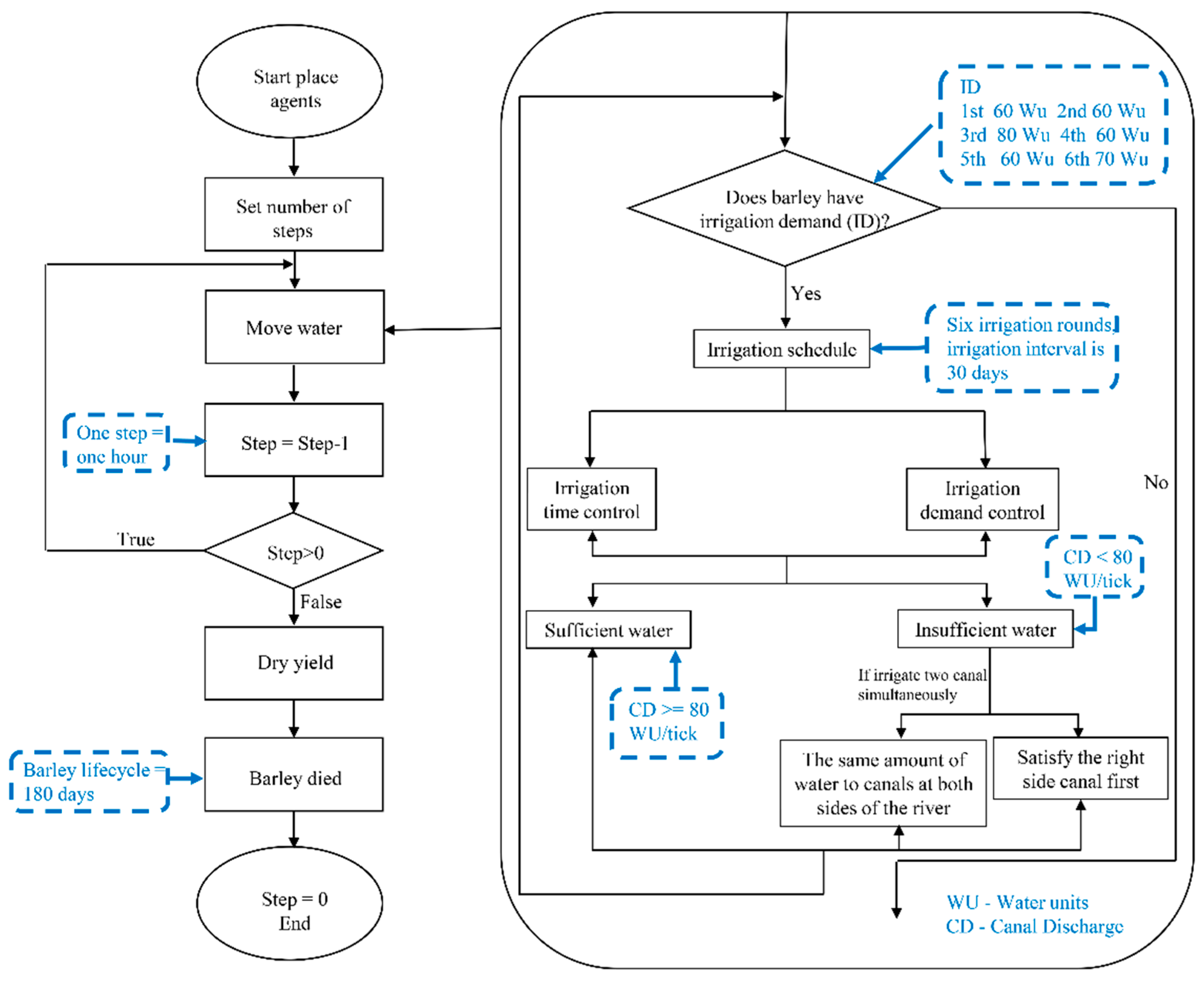
IRABM simulates the interactions of irrigation-related, non-human agents, which represent human choices, and as such human agents, as well. There are two main processes: the irrigation procedure and the water allocation procedure, Barley growth and water dynamics are updated at a hourly time step (Figure 1). At the end of the simulation, the dry yields of barley for all farms are given.
2.2. Model Design Concepts
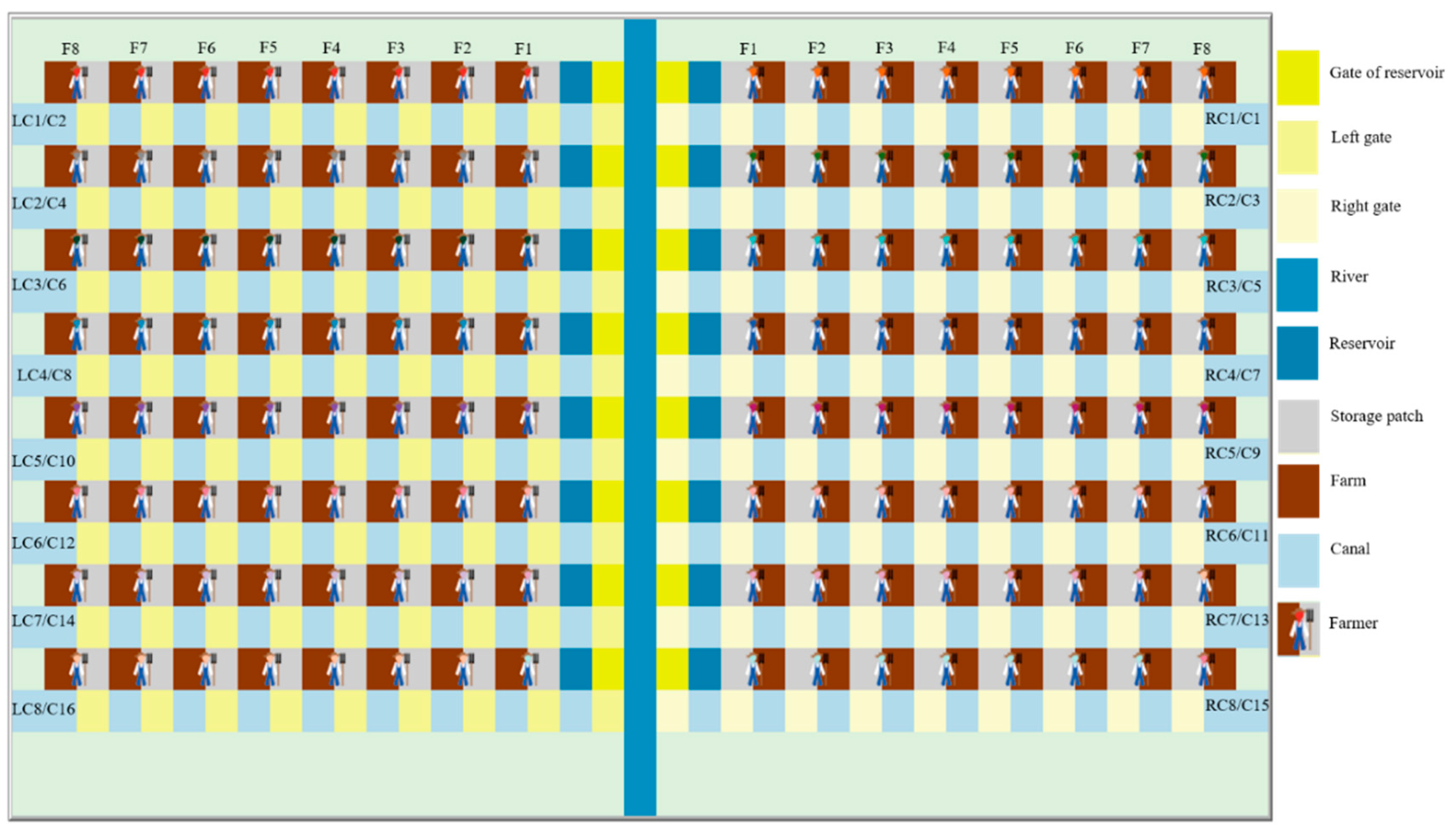
We designed a simplified layout for the irrigation system: one river feeds sixteen canals, with 8 farmers along each canal, with each farmer managing one farm (Figure 2). Hydrological processes such as rainfall, evaporation and evapotranspiration are reflected in water demands at farm level and water availability in the river. Drainage is not included either. River, canals, and gates are assumed to have constant shapes or profiles. Artificial water units (WU) were used in order to mimic these physical processes. Water units flow through the river and canals with constant velocity: water units move one cell per time step (tick). The main river flows along the head gates of the canals until eventually the river passes the last canal and remaining water flows out. The canal flow goes through the gates of the farmers, until water finally passes the last farmer and flows out. At the head gates, water has the possibility to flow into the canals; at the gates, the farmers have the possibility to withdraw water from the canal. We set a range of capacities to river, head gate, canal, and farm gates. We gave all farms a size of 1 hectare, with farms next to each other sharing similar soils.
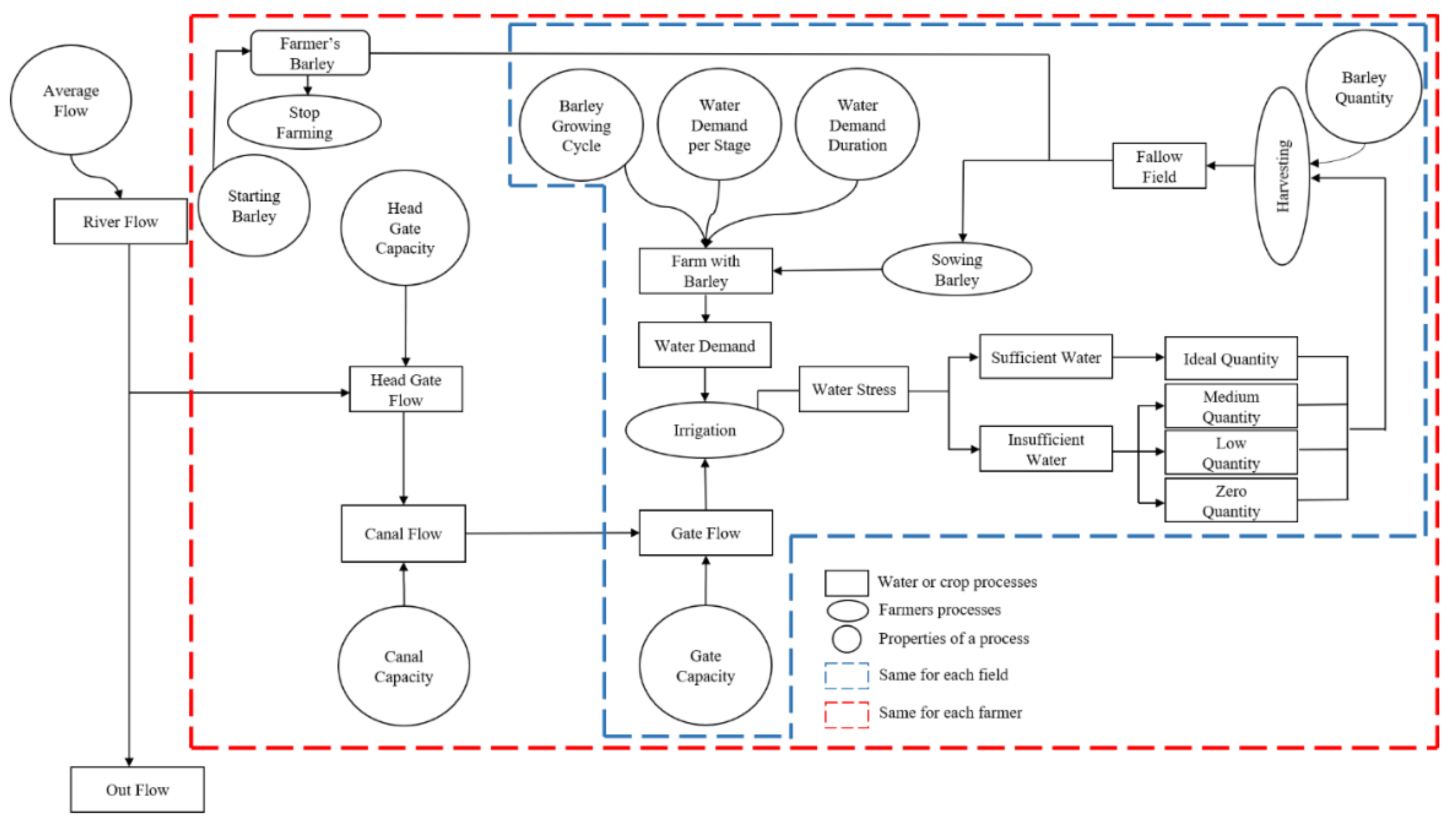
Figure 3 shows the entire modelling concept. Water from the main river (River Discharge RD) flows through canal head gates (Canal Discharge CD), and flows via these canals through farmers’ gates (Gate Capacity GC) to the farms. For each time step, farms have a current water demand, based on its history of receiving water. If there is not enough water to fulfil the water demand, barley will have water stress. Too much water stress results in reduced harvest quantities. This reduction is schematised in three steps: ideal-medium, medium-poor, poor-none (copied from the Irrigation Management Game [31]); see Appendix C). After the growing season, the model farmer will harvest. After harvesting, farms stay fallow until the next growing season.
2.3. Irrigation Schedule
An irrigation schedule is important to link irrigation-water management to (improvement of) crop productivity. A relatively simple calculation method [47] was applied, linking the depth of irrigation application and the calculated irrigation water need (IN) of barley over the growing season (Appendix B). Based on the calculation, we defined six irrigation applications (irrigation rounds) over one complete barley growth period—180 days, with an irrigation interval of 30 days. We also calculate the irrigation demand at each application as 60 WU, 60 WU, 80 WU, 60 WU, 60 WU, and 70 WU, respectively. The irrigation schedule represents farmers decisions when to open and close their gates according to their irrigation requests. The irrigation time per farm will impact barley yields on the farm, as irrigation time is directly linked to the water volume that crops receive. The same time may influence other farms, when bringing water to one farm lowers the available time for other farms. With our 30 days irrigation period, 1.5 days of irrigation time per canal is a realistic maximum time to irrigate one canal without disturbing others, when all 16 canals are to be irrigated one after the other. In the model, irrigation time IT is set at 1 day, 1.5, 2, 3, and 3.5 days, respectively, when irrigating two canals per tick.
2.4. Scenarios
Modelling of interactions between human agents and hydraulic variables can improve our understanding of how irrigation systems emerge within a specific human-water environment. As we aimed to compare how different irrigation controls can influence barley yields, we defined two types of possible water flow control. Time Control (TC) allocates to each canal a certain irrigation time, while Demand Control (DC) moves the water from one canal to the next only after the last farmer of the upper canal has satisfied the water demand. Furthermore, if water is scarce and RD cannot meet the water demand of the canals at both sides of the river simultaneously, a distinction is made between allocating the same amount of water to canals at the two sides of the river or satisfying the demand of canals on one side (right) first.
Given our available varied river discharges (RD), the number of canals being irrigated at the same time, two types of irrigation control (TC and DC), and a series of farmers’ gate capacities (GC), there are 840 possible scenarios in IRABM’s current version. The hydraulic characteristics of the scenarios were reflected in water agents (water units) and may indicate the coordination of farmers’ irrigation request and water availability. For all scenarios, water availability was expected as sufficient water and insufficient water on the levels of the whole system, canal, and farmer. These scenarios show the potential adaptation options for users in this model. Each scenario has been run for a single season of barley. Although several random functions are included in the algorithm of NetLogo, there are no random procedures in this model. With procedures predefined, following the design routine, scenarios have been repeated 3 times in order to estimate the outputs’ variability. For stochastic models 3 replications seem rather low, but with each procedure being predefined, we argue that 3 runs are enough for this study. Table 1 provides an overview of the parameters used in each scenario.
3. Results
Given the rather high number of scenarios, this paper provides a set of representative results to demonstrate IRABMs potential. This will show how the original features of this model, through the use of scenarios, can be used (as a realistic modelling basis) to explore irrigation performance. In terms of water availability for the whole system, the threshold of available RD is 160 WU/tick for scenarios irrigating two canals per time step, whereas it is 80 WU/tick when water is provided to one canal per time step. If the amount of available water for each canal is above or equal to the threshold, all farmers receive a certain amount of water to produce yields; if not, some or more even all farmers will face water stress. It is useful to mention that the maximum yields of each canal and each farmer are 24 ton and 3 ton in these simulations, respectively.
3.1. Abundant Water Availability
3.1.1. Irrigation Demand Control
When enough water is available, most farmers and canals gained optimal yields both when irrigating one canal and irrigating two canals simultaneously. Practically all canals gained optimal yields for GCs above 2 WU/tick. However, downstream canals and some middle-stream canals gain lower yields (or even did not have yields) for low GCs of 2 and 1 WU/tick (Figure 4). Irrigating two canals per tick resulted in canals and farmers gaining optimal yields for all GCs, except for GC = 1 WU/tick—with the farmers along the last two canals gaining half of the optimal yield (1.5 ton). When only one canal is irrigated, middle stream canals also start to be affected by the relatively low GC. Some farmers cannot even survive—as no yields at all.
There is no difference in yields in the system under DC when irrigating two canals simultaneously or one canal at the time for higher gate capacities. Apparently, the available RD can be transferred to all canals and farms. There is a difference, however, between canals, with downstream canals gaining lower yields, and, occasionally, even no yields at all—with lower GCs of 1 and 2 WU/tick, when most of the upstream canals still gained the optimal yields. Comparing irrigating two canals and one canal per tick, the former one results in higher and more constant yields for farmers located in the middle-stream and downstream canals for GC at 1 and 2 WU/tick. No matter how many canals are irrigated at the same time, there is almost no difference in yields among farmers located along the same canal.
3.1.2. Irrigation Time Control
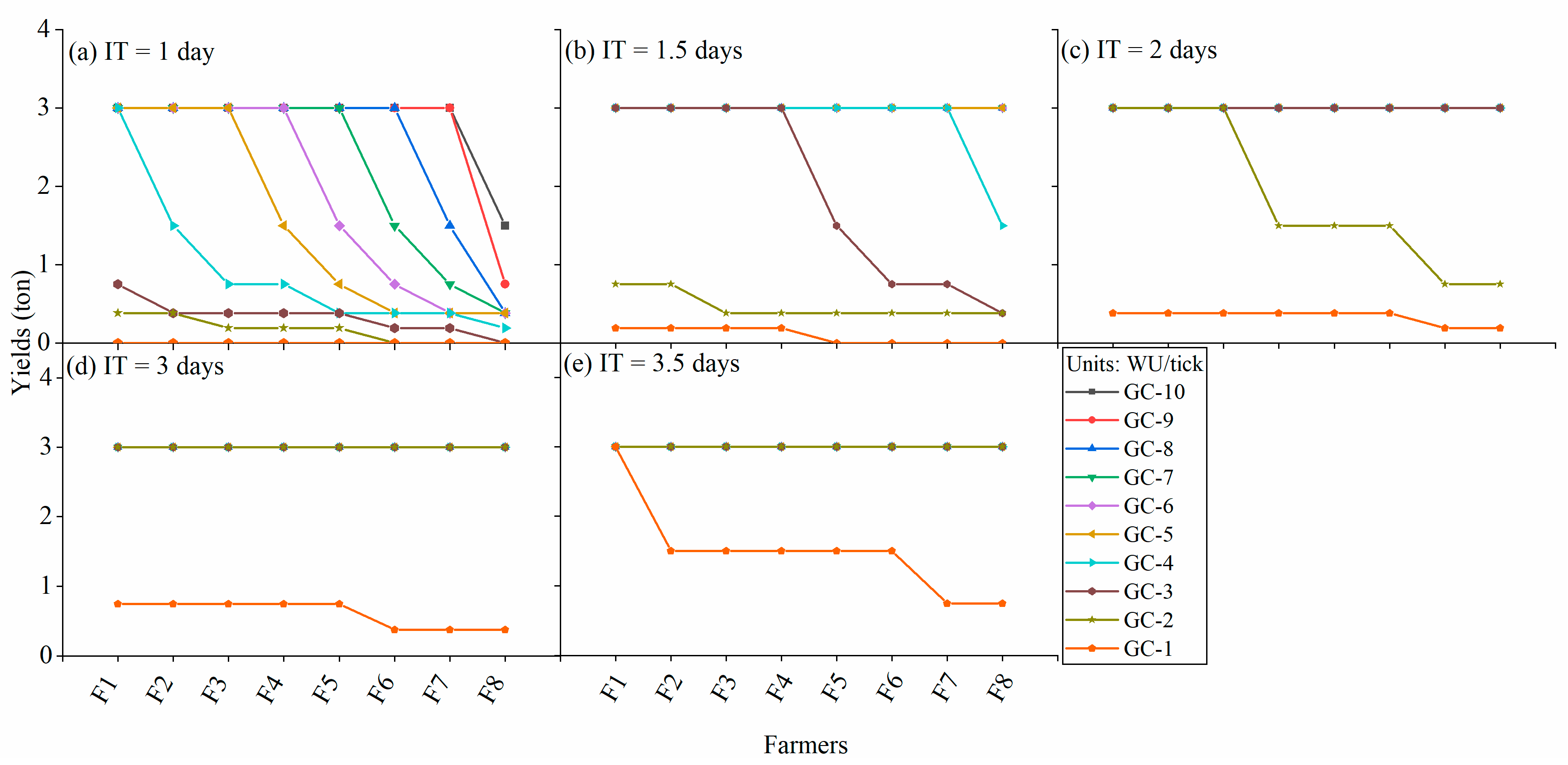
The results make it obvious that barley yields increased with the extension of IT and higher GC, again with sufficient RD (Figure 5). All farmers’ yields are shown in this figure: given the fixed time period, it is expected and easily observed that all canals have the same yields and yield distribution per farm under each combination of IT and GC. The most upstream farmer is the most productive one throughout, except for when GC = 1 WU/tick and IT= 1 day, when no farmer has a harvest. Irrigating two canals per tick creates more IT per canal and as such higher yields. With IT above one day, higher GCs resulted in very stable yields—with most farmers gaining optimal yields. The longest IT (3.5 days) resulted in high yields in general, but, above all, in a more equal yield distribution among farmers.
3.2. Abundant Water Availability
When the irrigation system is facing water stress, results become more diverse. Within the two canals’ perspective, we tested two water allocation strategies. Strategy one allocates the same flow to both canals, strategy two fulfils the gate capacity of the right canal first and sends the remaining water to the left canal.
3.2.1. Irrigation Demand Control
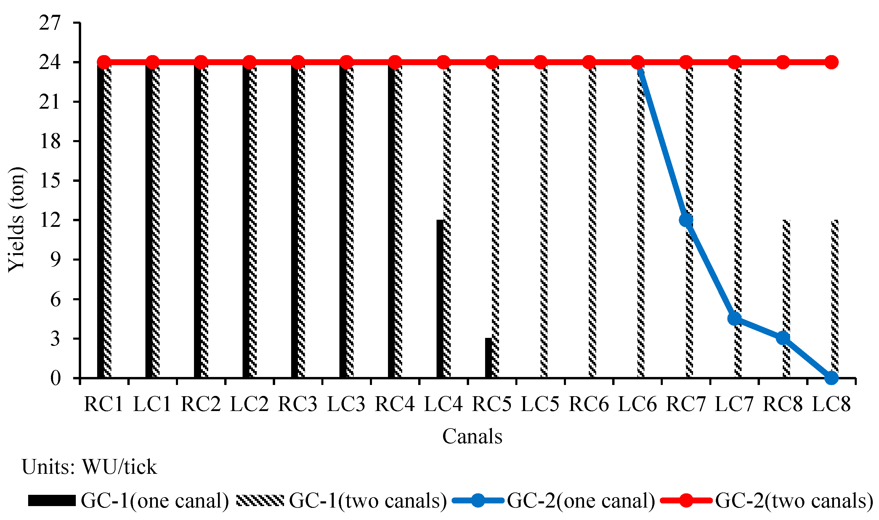
With insufficient water, results show that either all canals had yields or only a few canals had yields—with yields only existing along the first two canals, or only found along the first right canal. When canals have yields, they are always the same for all canals. Therefore, Figure 6 only shows yields of the first two canals. Actually, in most scenarios many canals could not produce yields. This is a consequence of the experiment model design: if water cannot flow to the last farmer in the first right canal, which means that the demand of that canal is not met, (farmers along) the next canals never receive water, even there is plenty of time left.
Under the strategy of prioritizing the right canal and with CD ≤ 80 WU/tick, only the first right canal can produce yields. If water is delivered to farms (farmers), most of them receive the desired water, which results in ideal yields. In case the last farmer along the upper canal stays without yields, however, no farmer along the lower canals can produce yields. Different GC thresholds were observed for different canal discharges in terms of yields for all irrigation strategies: either all canals gained yields with GCs below the threshold, or only the RC1 and LC1 canals gained yields when the GC was equal to or higher than the threshold. Generally, yields of RC1 and LC1 are lower than 24 ton means the GC threshold has reached, which also demonstrates that the rest canals are without yields. Figure 6 illustrates GC thresholds are 9, 6, 3, 2, and 1 WU/tick for canal discharges of 60, 40, 20, 10, and 5 WU/tick, respectively. Moreover, for GCs equal to or above the threshold, the total yield of each canal decreases and the number of farmers gaining yields declines. Higher GCs result in water not reaching the most downstream farmer of a canal, and in the demand setting of the model, this blocks the flow going through. If the GC is lower than the threshold—when water can flow to the downstream and the full irrigation time can be used—the results of each canal or each farmer are similar to those for settings with sufficient water. In other words, reducing water use of upstream farmers is beneficial for everyone in the system when water is scarce.
Allocating the same amount of water to two sides, i.e., splitting the available RD, gave better results in terms of yields, as the GC threshold is higher and more canals and farmers gain yields. The most important observation, however, when comparing the results of demand control for settings with sufficient and insufficient water, is that the demand setting of the model brings a typical irrigation dilemma to the front. For lower RDs with higher GCs, water could be kept from flowing further than the first canal(s), which results in downstream canals having no yields—unless the upstream farmers limit their water use, which does not necessarily lower their own yields. Furthermore, in DC scenarios, the main difference in yields exists between canals, not between farmers. Both for canals and farmers, the main factors affecting yields are RD, GC, and canals’ location.
3.2.2. Irrigation Time Control
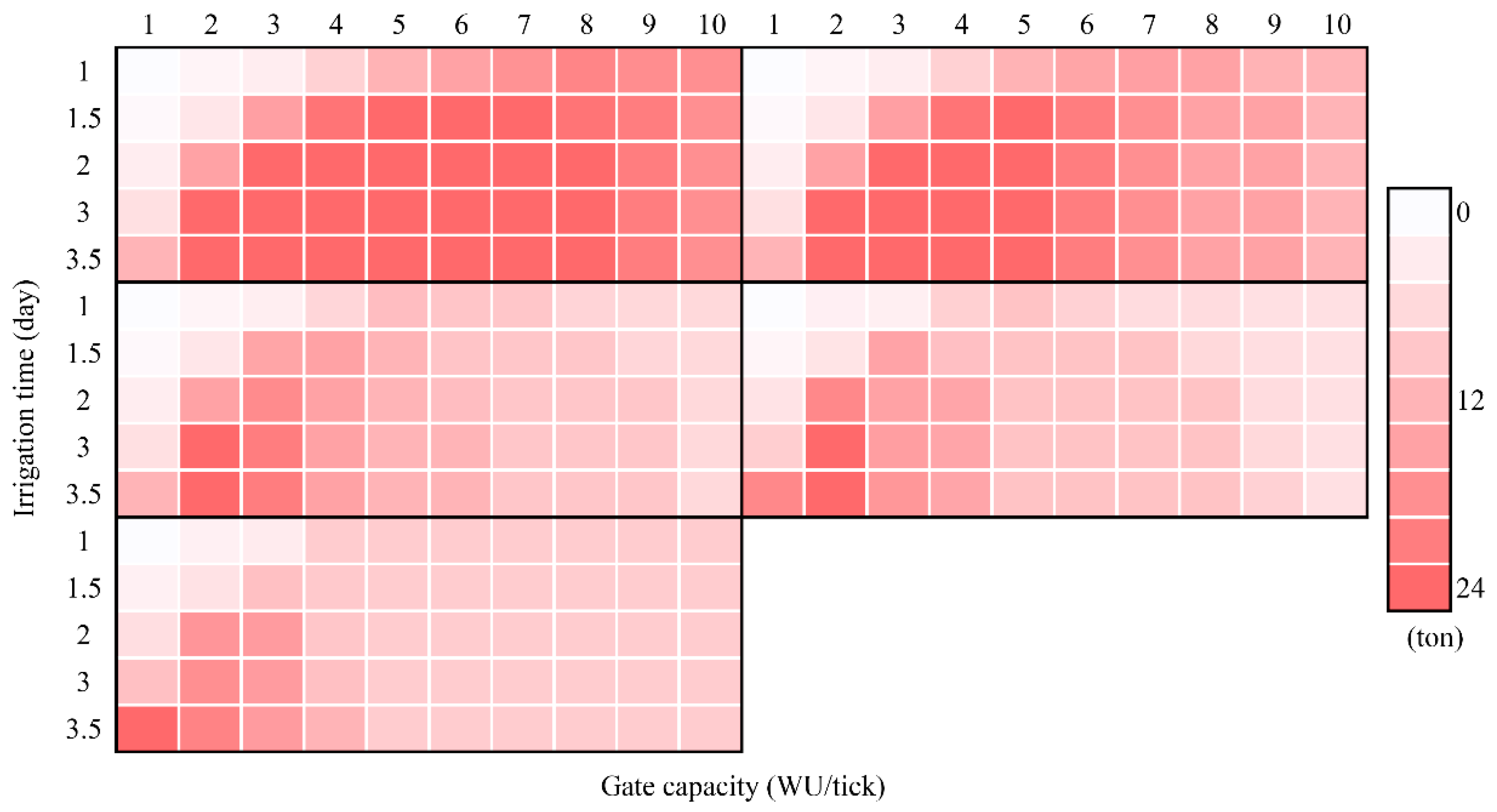
The GC threshold is also observed for TC with insufficient water: higher GCs generate relatively lower yields. The pattern is that shorter ITs generate a higher GC threshold, while longer ITs generate a lower threshold (Figure 7). GC thresholds decreased with decreasing RD and varied with different IT. In addition, tipping points for GCs are observed: yields decrease rather dramatically with specific decreases in GC. Usually, the tipping point is lower than 5 WU/tick, and decreases with extended IT. If GC = 1 WU/tick and IT = 1 day, barley yields zero ton, no matter how RD varies. Concerning different water distribution strategies, all canals act the same when distributing the same amount of water to each side. The prioritizing of right canals’ demands results in all right canals and all left canals, respectively, realizing similar yields—with the second strategy leaving all left side canals without harvest for RD ≤ 80 WU/tick, as there is no water left for them.
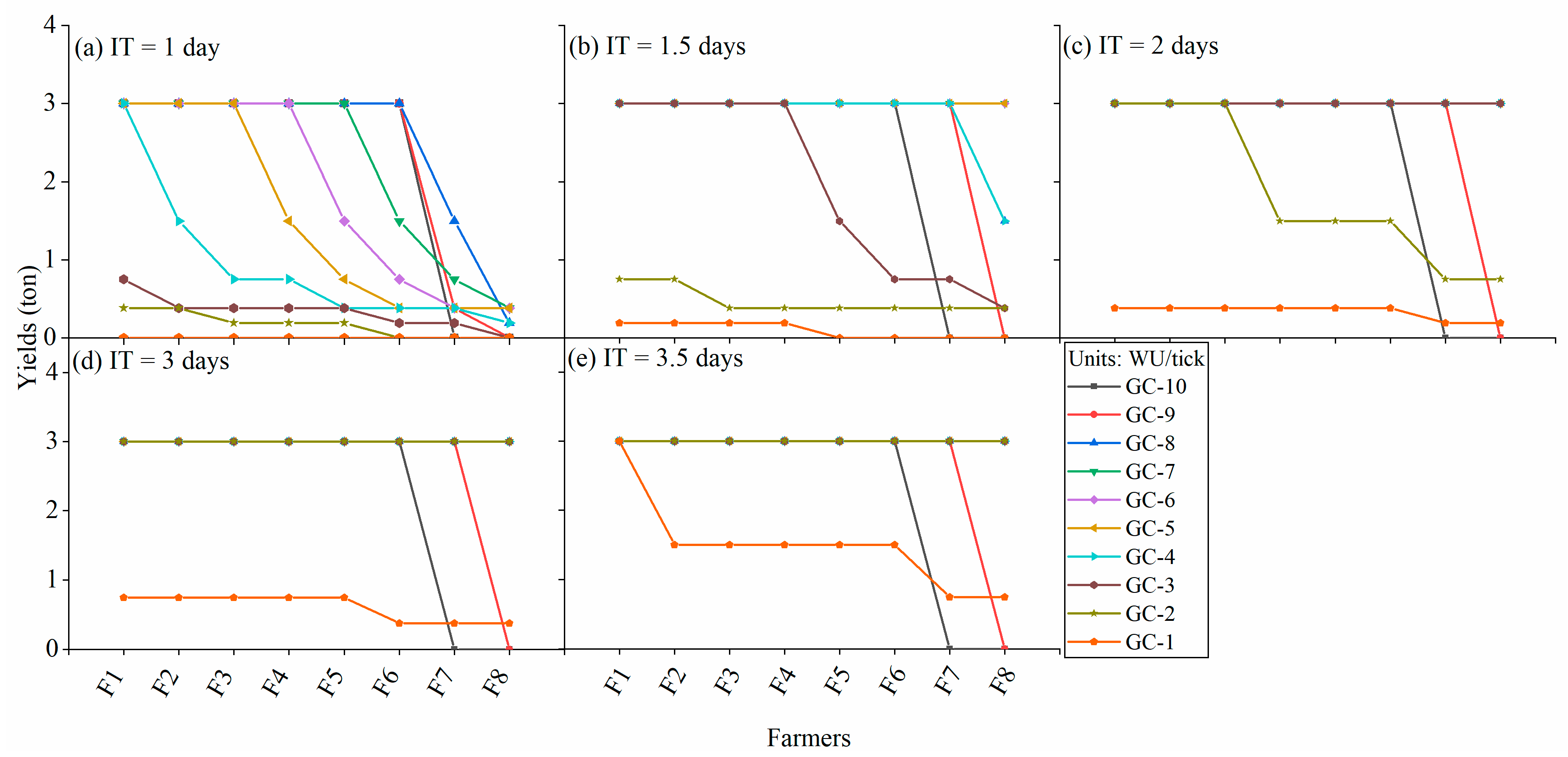
As one example, Figure 8 shows farmers’ yields when CD = 60 WU/tick, which is the best harvest situation among the insufficient water scenarios. In Figure 8, we see that water cannot flow to the downstream farmers with GC = 9 and 10 WU/tick for all ITs. Furthermore, longer IT and higher GC (excluding 9 and 10 WU/tick) can generate higher yields, but extremely low GC, especially with shorter IT, and can lead to the collapse of farmers. The number of farmers gaining yields declines and the yields of each canal decrease with rising GC, but at least each canal has yields. For lower GCs, the (bad) results of canals and farmers are similar to situations with sufficient water supply. Overall, most downstream farmers, some middle-stream farmers, and even several upstream farmers stay without harvest at all—even in scenarios with the longest IT time and higher GC, which results in no yields for farmers relatively downstream and reduces canals’ yields. Whatever the combination of factors, it is apparent that the downstream farmers along a canal are affected the most, followed by the middle-stream and upstream farmers.
In summary, similar dynamics can be observed for time-control scenarios that irrigate one canal and two canals per tick, both for yields of canals and farmers. When canal discharges are at least 80 WU/tick, barley yields increase with prolonging IT and rising GC. Both for canals and farmers, yields are high and stable when IT is above 1.5 days. However, and second, with insufficient water, but GCs stay relatively high, downstream farmers along a canal have no yields and the total yield of a canal is reduced. Moreover, irrigating two canals simultaneously will further reduce the canal discharge. This suggests that irrigating one canal at the same time could be better than irrigating two canals at the same time, when prioritizing the benefits of the community above the individuals. Third, it can be easily observed that there is no difference between canals under each sub-scenario, but there are differences between the upstream, middle-stream and downstream farmers along a canal. These results indicate that IT, GC, and RD are factors that affect canals and farmers’ yields, while farmers’ location also affects farmer’s yields.
3.3. Water Control Patterns
When the irrigation system is facing water stress, results become more diverse. Within the two canals’ perspective, we tested two water allocation strategies. Strategy one allocates the same flow to both canals; strategy two fulfils the gate capacity of the right canal first and sends the remaining water to the left canal.
The comparison of all sub-scenarios suggests that if the irrigation system has sufficient water supply, DC and irrigating two canals per time step is the best choice. In case of water deficiency, TC would be the better choice, as at least more canals and farmers gained yields, and yields could be managed by managing irrigation time. For DC, some differences in yields are created between upstream, middle-stream, and downstream canals, but there is not much difference between farmers located at the same canal. In contrast, with TC, there is no difference in yields between canals, but there are differences between the upstream, middle-stream, and downstream farmers within the same canal.
When the irrigation system is facing severe water stress, GC could be the most important factor affecting yields. Higher GCs bring benefit to the upstream farmers only. To benefit more farmers, which also would be beneficial for the whole irrigation system in terms of yields—and does not go against the benefit for upstream farmers at all—lower GCs should be used. The number of canals irrigated per tick is also a major factor, which could affect irrigation decisions when facing water deficiency. To create benefits for more farmers, irrigating one canal per time step would work better. In order to create higher profits for some individuals, irrigating two canals simultaneously works better.
Lower RDs with GCs result in lower yields per canal and fewer farmers gaining yields, because of the water flow patterns that are created to both irrigation controls. Table 2 summarizes when water can flow to which farmer for all CD situations under all RD scenarios. If CD is lower than 80 WU/tick, there is a GC threshold that blocks water from flowing to farmers downstream along a canal. GCs above the threshold block water flowing to the downstream. The gate thresholds are 9, 6, 3, 2, and 1 WU/tick for CDs at 60, 40, 20, 10, and 5 WU//tick, respectively. The threshold value decreases with lower canal discharges. This implies that if water availability is lower, only low GCs make water flow downstream.
3.4. Patterns of Yield
There are 840 sub-scenarios in this experimental model. A total of 153 sub-scenarios gain the optimal barley yields of 384 ton, or 3 ton per farmer, whereas 12 sub-scenarios gain no yields at all. In terms of total yields for the irrigation system, 8% of the sub-scenarios gain exactly halve of the maximum yields, or 192 ton. Over 50% of the sub-scenarios give total yields below 192 ton, while 35% gain yields over 192 ton. Sub-scenarios that result in the same total yields, however, have different underlying interactions between canals and farms/farmers. Only the total yields of 384 and 0 ton, respectively, indicate automatically that the whole irrigation system—all canals and farmers—did the same things in terms of water distribution.
Table 3 shows some examples of different water distribution activities that resulted in the same total yields for the system as a whole. Even for these low overall yields, different scenarios can be identified.
- Cases 1–4: the same low total yields are the result of different results per canal and between farmers: canals have the same yields, but farmers do not. In case 4, the first two farmers along each canal harvest 0.38 ton barley, but the last six farmers gain nothing. In cases 1 to 3, the first four farmers along canals yield 0.19 ton, with the rest of farmers harvesting nothing.
- Case 5–6: in case 5, each canal yields 3 ton, because each first farmer could gain 3 ton barley, while the others are left without harvest. For case 6, each right canal gains 6 ton barley, but the left canals gain nothing. Actually, the first two farmers along each right canal gain 3 ton barley, while the other farmers harvest nothing.
- Case 7–8: in case 7, only the first two canals gain yields (18 ton), whereas the other canals remain without yields. Case 8 shows each right canal gaining 4.5 ton, but the left canals have no yields. In terms of difference between farmers, case 7 allows the first six farmers yields of 3 ton each, but the last two farmers gain nothing. Case 8 shows yields of 3 and 1.5 ton for first and second farmer along the right canals, respectively, but the left-canal farmers are bankrupted.
4. Summary and Discussion
The founding principle of the IRABM model is the irrigation cycle being divided into six irrigation rounds, according to barley growth stages, with irrigation options being simulated separately in each round with varied scenarios combining available water, canal and gate settings and control methods. The results clarify how and why irrigation patterns (can) emerge when agents act in an irrigation setting. The way(s) the different model agents (model parameter) influence barley yields can be analysed. The model outputs have allowed several main findings to be defined:
- Demand control gives better results in terms of yields than time control, when there is sufficient water in the river.
- Time control should be the first choice when our irrigation system faces water deficiency.
- Barley yields generally increase when irrigation time and/or river discharge are extended.
- Tipping points of gate capacity resulting in differences in yields can be observed.
- Yields do not change linearly with changing gate capacities but show threshold behaviour.
Some results can be understood as artefacts of our own model settings. For example, in a situation with irrigation demand control, a relatively high gate capacity, and insufficient water in the river, it can be easily observed that yields only exist along the first level canals. This is the direct consequence of the current model design settings, with the control rule only allowing water to flow to a next canal when the last farmer along the upstream canal receives the required water. This may be seen as the extreme version of an expected outcome that, in terms of locations along the canals, downstream farmers run much more risk to be negatively affected in their water availability—especially those farmers that are downstream in the more downstream canals. Similarly, the downstream farmers along a canal are affected the most in the case of time control.
There is a rather important aspect, however, concerning the effect of the position of farmers in relation to how water moves from upstream to downstream. Through changing gate capacities—the management of flows to the farms—we showed that in situations with sufficient water in the system, higher gate capacities generate higher yields for farmers in the whole system. When there is insufficient water in the river, however, higher gate capacities only benefit upstream farmers, whereas lower gate capacities could benefit both upstream and more downstream farmers—and, as a consequence, the whole system.
Therefore, this experimental model generates an emerging setting that we did not explicitly build in, but that relates closely to real-world irrigation systems. In real irrigation management, upstream farmers often take more water than allowed, even when there is insufficient water on a system level, resulting in downstream farmers facing further water stress. But if every farmer’s gate capacity is kept low enough, water could probably be allocated to each farmer, which should result in everyone at least receiving a certain amount of water.
4.1. IRABM’s Engagement with Other Studies
IRABM aims to construct an ABM framework to explore varied scenarios to mimic the operation of an irrigation system and the longer-term emergence of irrigated settings. Obviously, we are not the first to build an irrigation-related ABM to do just that. As already mentioned in the Introduction, Tamburino et al. [16] built an ABM to mimic a smallholder farming system with conditional environmental attributes to explore the interactions between water courses, humans, and crops. One of their main focus issues was farmers’ behaviour in relation to group activities. Hu and Beattie [15] developed an ABM using a two-stage optimization strategy to guide farmers to make an optimal decision on choosing crop and groundwater irrigation. Their results proved the viability of strategies resulting in higher crop yields and slower groundwater depletion—an issue similar to the canal sharing dilemma, mentioned earlier. Anthony and Birendra [14] developed an ABM to explore its ability to manage water distribution strategies in New Zealand, which suggested that significant water savings were possible. Barreteau et al. [48] built the SHADOC model, a multi-agent simulation of the dynamics of an irrigation system in the Senegal River Valley. With scenarios defined as an environment plus a set of individual and group rules, their results suggest that their simulations can be used to evaluate the viability of irrigation systems, as well as provide a new approach to the study of such systems.
The current IRABM version was built to analyse the interactions among non-human model agents that could both represent human activity and non-human realism: river discharge, gate capacity, irrigation time, farmers’ location, and barley yields. This digital experiment model provides opportunities to study complex irrigation-system dynamics from a new perspective. One of the main problems of the “irrigation dilemma” is the inequality between upstream and downstream farmers’ ability to access water when they share a common water resource [49]. Janssen et al. [11] used an experiment with constrained communication and limited information to study inequalities of water access. Their research illustrates that lack of communication among farmers could cause an imbalance between upstream and downstream farmers’ investments and earnings. Our model experiments, with model farmers that have no means of feedback (communication), yet, confirms that the “irrigation dilemma” can be caused by upstream farmers simply responding to water availability—they do not need to steal water, just not knowing what happens downstream would be sufficient to leave downstream farmers with less possibilities to access water, especially when there is water scarcity, resulting in downstream farmers—and the system as a whole—gaining less earnings.
As already mentioned, this phenomenon is a genuine emerging result of the model setup, as we did not build-in this kind of “emergence” using something such as the ODD protocol. We did not specify that upstream users had to take water, we studied what happened when they did. We did not define what type of emergence our model should be based upon, as emergence that is already known is not really emergence. What we did find, however, when applying a model setup that was realistic enough to catch water flow behaviour, and yet simple enough to run multiple scenarios, was threshold behaviour in the system, which is exactly what one would expect in realistic irrigation settings. With much of the ABM work available explicitly defining the expected results or key outputs beforehand through the ODD protocol [43,44,45,50,51], we would like to argue that “emergence” should be a new phenomenon in a model. Results such as upstream farmers taking water at the cost of downstream farmers, predictable as it may be, should always be surprisingly (“naturally”) emerging from a reliable and robust ABM—without being pre-defined in the ODD protocol. Similarly, there is no specific adaptation in this model as all settings are predefined, although the performance of irrigation-related non-human agents already represents potential adaptations. Different water allocation strategies show the adaptation of varying river discharging, the settings of the gate (capacity) reflect the adaptation of water supply and irrigation schedule, and the yields of barley represent the adaptation of different water distribution strategies. Consequently, potential adaptation phenomena can go through model agents, even in a model with predetermined settings.
One could argue that IRABM goes against the trend that current ABMs of the human-environmental systems, become increasing complex [38]. For instance, Bithell and Brasington [52] developed a coupled modelling system that consists of several sub-models (ABM, individual-based and hydrological) to simulated land-use change. Arnold et al. [53] coupled an ABM with a hydrological model in a multi-agent farm decision and production simulation to quantify the economic importance of irrigation water reuse. Jaxa-Rozen et al. [54] combined ABM with MODFLOW/SEAWAT geo-hydrological modelling to study Aquifer Thermal Energy. The interesting results notwithstanding, we would suggest that irrigation systems are complicated and dynamic systems, because of interactions between (non)human agents on small temporal and spatial scales. As the effects of these small steps can be approached with a relative certainty, IRABM only needs to involve simplified hydrological and hydraulic processes, including synthesised data, instead of using coupled ABM with crop or hydrology/hydraulic simulations on larger temporal or spatial scales. The objective of this study was to show how IRABM can represent and study relevant human-water system interactions without predefining them. We think we have shown that IRABM provides the flexibility required to allow dynamical agents’ actions. As such, we plan further model steps, which both involve more complicated feedback mechanisms between and more accurate methodologies to represent certain agencies.
4.2. IRABM’s Next Steps
The experimental model discussed is to be developed for further studies, especially focusing on how agents’ actions can change when results (such as yields) become known to model agents and key model parameters are varied. The base model was designed using the principles laid out in Ertsen [18,39]: the non-human agents, such as canals, gates and crops, shaped the temporal and spatial options of the human agents. As mentioned in the Introduction, we are particularly keen to use our model setup to study longer-term irrigation development in ancient Mesopotamia. Communication and cooperation were crucial in Mesopotamia to create successful and efficient irrigation works [55,56], but how such cooperation and communication emerged is less certain. In the current setup, human agency is represented by setting the amount of water flowing through gates. While not including human decisions, as such, in the model, we have been able to illustrate how the interactions among IRABM model agents show possible effects of agent interactions and tensions between goals of individuals versus the overall community. There is no communication and corporation in the current IRABM setup, but upstream and downstream farmers already compete for the water according to their location.
Building options for interactions among farmers is a way to increase the benefit of the downstream farmers and even the whole system in the model. Real-world decision making is influenced by many complicated factors that must be simplified in any modelling approach. The next IRABM setup will allow for the consideration of irrigation decisions on crop choice, irrigation forecast, and water allocation. IRABM’s barley irrigation schedule is divided into six irrigation rounds, with each round having a regular time period. As our running periods remained short, this level of detail could be used. We consider condensing the whole barley growing period into one irrigation season, as this may provide a quicker computation routine, which would be beneficial for multiple-year runs, but this would lose the effect of decision making and water distribution within a season. Whichever seasonal setup we choose to work with, multiple-year runs bring us to the issue of memory in the model, for example, in the shape of “irrigation memory” or “available water memory”. We are looking into options to create possible feedbacks between farmers based on these memories—possibly in different combinations, including knowing the results of other farmers. We could extend this work by considering more irrigation-related factors or adding different crops to optimize water allocation strategies and crop yields to simulate farmers’ decision making.
With these inputs, we move closer to the coupled models, mentioned earlier. These models might face challenges, such as modelling design, processes of data change, and results interpretation, but these models can capture complex behaviours and be friendly to decision-making support, scenarios analysis, and forecasting capacity [38,54,57]. We could still decide to move towards a coupled model, with IRABM being enhanced with a crop-growth model and hydrological/hydraulic model, but for the moment we plan to stay within the NetLogo environment.
We showed the flexibility of the IRABM framework of using non-human agents to present human agents and demonstrated its ability to simulate the interactions of irrigation-related agents in an irrigation system. It provides an alternative perspective to simulate the human-water system and is friendly for non-technical stakeholders. The IRABM is already able to simulate the effects of decisions, and decisions can be directly linked to current model elements (canals, gates and farms); it is a promising tool that could be used as a framework to study both the operation of irrigation systems and the longer-term effects of this. We are planning to apply an extended IRABM to irrigation development in Mesopotamia. The IRABM is ready for more.
Author Contributions
Formal analysis, visualization, and writing—original draft preparation, D.L.; the designing of the model, methodology, and writing—review and editing, D.L. and M.W.E., supervision, M.W.E. All authors have read and agreed to the published version of the manuscript.
Funding
This work was supported by China Scholarship Council with the project reference number of 201806910044.
Institutional Review Board Statement
Not applicable.
Informed Consent Statement
Not applicable.
Data Availability Statement
Data sharing not applicable.
Conflicts of Interest
The authors declare no conflict of interest.
Appendix A. ODD Protocol
Appendix A.1. Purpose and Patterns
This research project develops an agent-based computational simulation to explore (the possibility of modelling) the operation of irrigation systems through (and illustrate) the interactions among agents, including several agents that are usually conceptualised as “related environment”. This will be achieved by creating a water system in NetLogo, to simulate the water-flow process from river to canal(s), and finally to the farm(s).
Barley yields at farms (the smallest spatial scale, representing individual farmers or families) are used to check the results of water distribution. Aggregating yields at the levels of canal or whole system allows exploring how specific irrigation strategies create patterns. These patterns reflect the results of interactions among the agents in this model. Barley yields are directly dependent on water distribution, as crop yields should respond to the changing irrigation measures [14,15,16]. Water distribution, in turn, is created by combinations of river discharge, irrigation control, gate capacity, irrigation time, and water allocation strategy.
Appendix A.2. Entities, State Variables and Scales
The environment of this simulation is a water system: one main river brings water to an irrigation system with farmers, canals, gates, and farms. Canals are built along the river, which is used as the transfer tool of water. Gates allow water to flow from the river into irrigation canals, and from canals to farm(s). There are gates at the junction of the river and canal (head gates), and at the junction of canals and farm (farmers’ gate).
Due to the semiarid climatic conditions, cultivated crops in south Mesopotamia have, and still are, heavily focused on winter cereals (barley and wheat), which are sown in October/November/December and harvested in March/April/May. Barley was the predominant crop in antiquity, as barley is more tolerant of alkaline soils compared to wheat. As it is more drought-resistant, barley is more productive in drier conditions. Barley provided the basic resource for beer, which was highly important in the diet in south Mesopotamia [41,58,59,60] Thus, barley is selected to be the object crop in this study.
The model consists of the following entities: river, canals, gates, farms, water managers, and farmers. There is one river, with eight canals. There are eight farmers along each canal; two farms belong to one farmer in this virtual irrigation system. All these entities are stationery but water is the only agent that can move through the model environment. The scale in NetLogo is 38×18 cells. Table A1 shows the state variables associated with these entities. There are two Boolean variables, that can be used to turn on or turn off processes. Other variables are integer.

Table A1.
The parameters used in this model.
| Model Variables | Lower Bound | Upper Bound | Units |
|---|---|---|---|
| Simulation Days | 0 | 365 | day |
| GateMaxFixed | 0 | 10 | WU |
| HGateMaxFixed | 0 | 80 | WU |
| Gate Limit? | off | On | \ |
| Hgate Limited? | off | On | \ |
| Qin, average | 10 | 200 | WU |
| StartBarley | 0 | 0.15 | ton |
| Barley harvest cycle | 0 | 180 | day |
| MaxStorageofStoregePatch | 0 | 80 | WU |
| IrrigationDemandPerTick | 0 | 10 | WU |
| First irrigation demand | 0 | 60 | WU |
| Second irrigation demand | 0 | 60 | WU |
| Third irrigation demand | 0 | 80 | WU |
| Fourth irrigation demand | 0 | 60 | WU |
| Fifth irrigation demand | 0 | 60 | WU |
| Sixth irrigation demand | 0 | 70 | WU |
| Barley yieldsY6 | 0 | 3 | ton |
| Barley yieldsY5 | 0 | 3 | ton |
| Barley yieldsY4 | 0 | 3 | ton |
| Barley yieldsY3 | 0 | 3 | ton |
| Barley yieldsY2 | 0 | 3 | ton |
| Barley yieldsY1 | 0 | 3 | ton |
The entities and their state variables are defined as follows:
- The river is the origin of the water resource. Water moves one cell per time step, whatever the inflow. The relevant variables are varied river discharges.
- Canals are transfer tools of water, transporting water from the river to farms. Water moves one cell per time step, organised with canal capacity.
- Gates control the water flow. Water moves one cell per time step, arranged by gate capacity.
- There are two types of farms in this model. One is with barley; another one is fallow—allowing for storage of irrigation water. The farms with barley have the variables: water demand, water stress, start barley, barley yields, harvest cycle, barley alive or not. The fallow farms have the variable: irrigation volume and storage capacity.
- Water managers propose water allocation strategies. Water allocation control, or irrigation water control, to canals can be achieved in two ways: time control and demand control.
- Water distribution strategies are shaped through river discharge, the number of canals irrigated simultaneously, and barley water demands.
- The farmers make choices on crop growing. Farmers may support the water allocating strategies in the system. They have the variable: irrigation demand.
Emergence—The primary outcome of this model is the yields of barley. This outcome emerges from how barley respond to varied river discharge and different irrigation strategies. As discussed in the results, this way of modelling actions does actually produce realistic emerging patterns, without predefining which patterns (or which specific relations) to take into account.
Adaptation—The options for the virtual water managers to adapt to water needs and availability are created in two ways. One is to define a water allocation strategy according to the river discharge, the other is to decide to open the gate or not—potentially following the farmers’ irrigation demands. The farmers’ adaptation strategies are to be based on the barley irrigation demand and received water distributed by water managers. Barley yields are adapted by received water.
Objectives—There are three main objectives in this model. Firstly, the objective of water managers is trying to meet the farmers’ water requirements. Secondly, the farmers’ objective is to make sure the barley grows in good quality. Lastly, the objective of the barley is to meet its water demand. The model runs, so far, show the outcome in relation to these goals; the fulfilling of the goals is not guiding the actions of the model agents yet.
Learning and prediction—The agents do not learn, as it is a one-year simulation. Once the simulation runs for numerous years, there are options to include learning actions among farmers and water managers. They could then make (better) decisions based on their previous experience. The same reasoning holds for predictions about future options. For instance, water managers can make water-allocating strategies ahead, while farmers can plan the irrigation schedule and make (better) decisions on barley sowing based on the previous experience.
Sensing—The main sensing behaviour in this model is the water flow pattern. Water can only flow from the river to the canal and finally to the farms and try to meet the barley irrigation demand.
Interaction—The decision making by the human agents is set in the different gate settings, which influences waters flow and barley production. Water managers and farmers interact with each other, in the sense that different gate settings result in different options to realize barley yields. At the moment, there is no realistic decision making available to model agents on water allocation strategies and gate openings (but decisions are represented by the performance of non-humans), nor is there an option for farmers to respond. As such, the implicit interaction in the model is that farmers accept the water managers’ decisions that come to them in terms of water input.
Stochasticity—There is no stochasticity in this model.
Collectives—The irrigation system itself is a collective of the actions of all agents. We consider barley yields of individual farmers, of a group of farmers along the same canal, and of the whole irrigation system, to explore how actions at different locations in the system affect the results in the system.
Observation—The ultimate purpose of this model is to explore how the irrigation related agents interact with each other, resulting in barley yields. Accordingly, the key output of the model is the barley yield of each farmer, which is closely related to another primary output, the amount of received water of each farm.
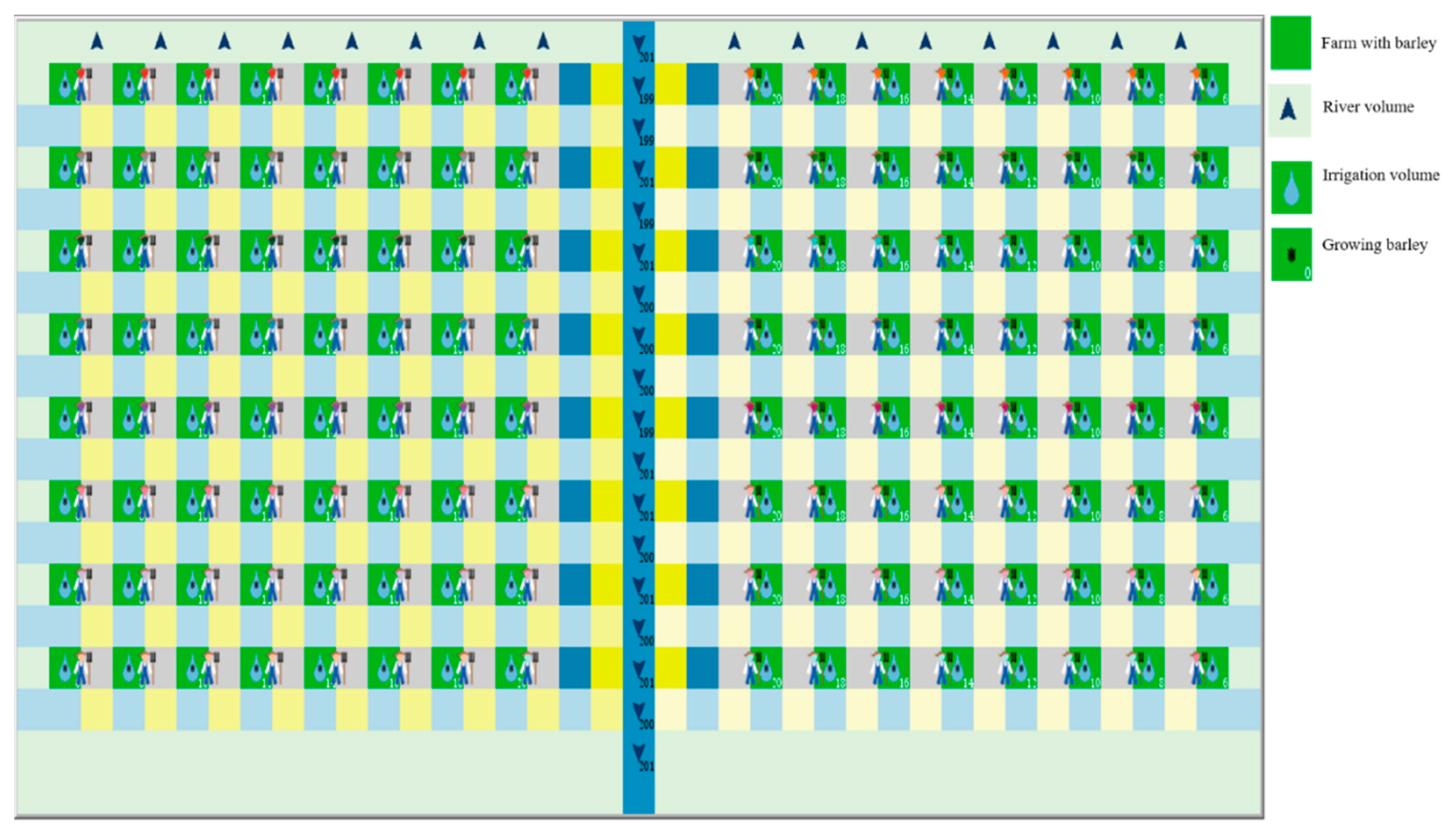
Initialization—At initial stage, each farmer has a certain amount of barley seed to ensure he/she can sow. The barley farm is brown at first, and it will change to green after sowing the barley. Each patch is empty at the beginning, except for the farmers who stand at the middle of two farms. When the model is running, the patches will be occupied by water volume, irrigation volume or barley (Figure A1).
Input data—There is no external input data.
Sub-models—The sub-model applied in this study is the irrigation schedule and the response of barley yields to supplied water.
Figure A1.
The model interface with running.

Appendix B. Irrigation Schedule
The irrigation schedule was calculated through the following logic:
Estimating net and gross irrigation depth (and)—The dominant soil type in Mesopotamia is clayey. Barley is a deep rooting crop. According to Brouwer et al. [47], this results in a of 60 mm. The gross irrigation depth can be estimated using the following equation:
where is the field application efficiency (%), 60 % was chosen in this research [47].
Estimating the IN over the total growing season—IN can be computed as follows:
where is the crop water demand for the th growing period (mm) and is the effective rainfall during the th period (mm). The total net IN during the total growing period is developed as:
where is the total growing period.
Estimating the number of irrigation applications over the total growing season—The number of irrigation applications () over the total growing season can be calculated as follows:
Estimating the irrigation interval (INT)—The INT is calculated in days and can be obtained as follows:
Appendix C. The Response of Barley Yields to Water Supply
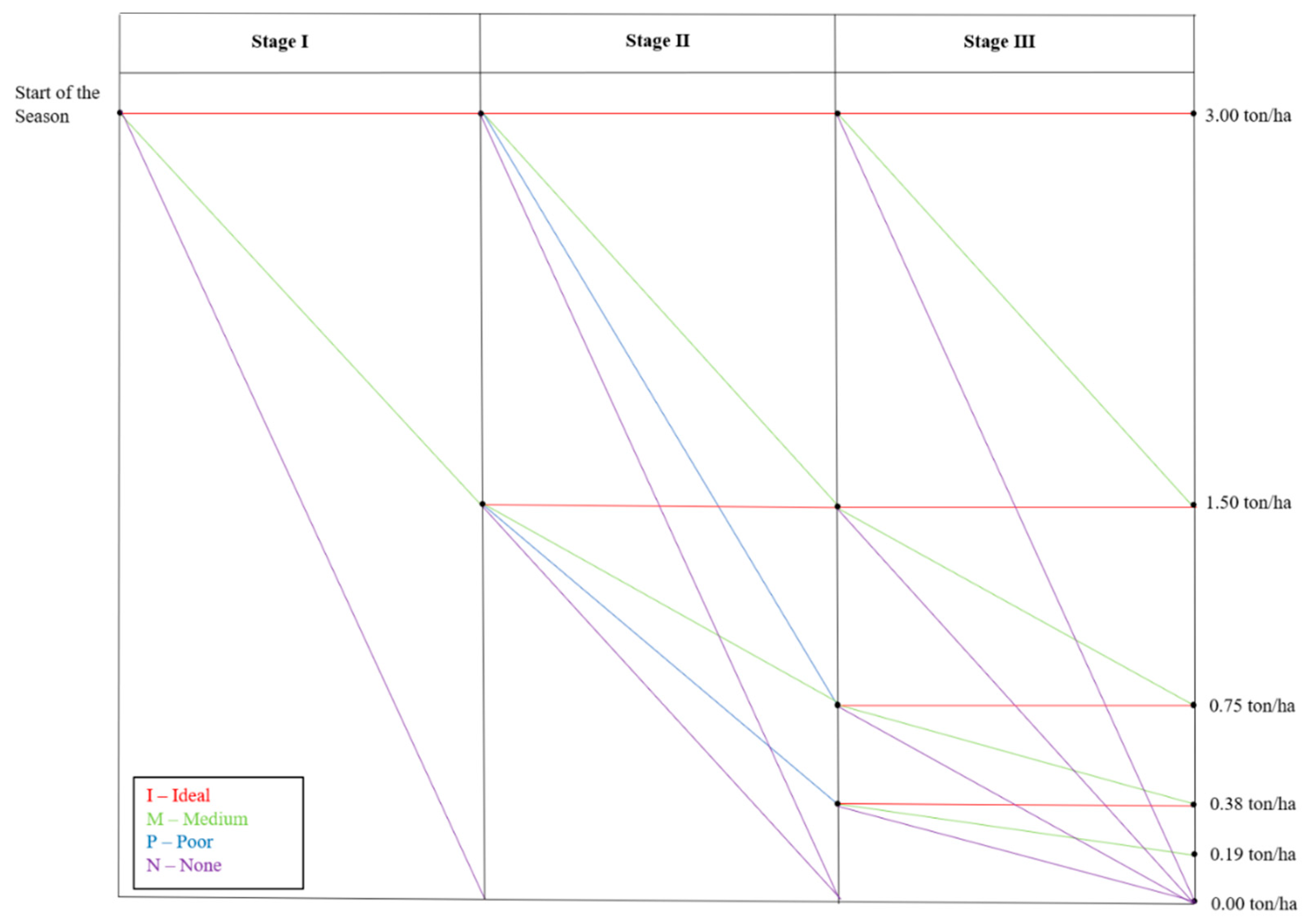
Table A2 and Figure A2 show the simplified water supplies to barley at each of three growing stages and divided into four levels: Ideal, Medium, Poor, and None, which present four levels of barley yields. From a simplification of reality: stage I includes irrigation round 1 and 2 (crop initial growing stage), stage II includes irrigation round 3 and 4 (crop middle growing stage), and stage III includes irrigation round 5 and 6 (crop late-growing stage). Calculation ratios of supplied water are taken from [32]: Ideal is 1.0; Medium is from 0.5 to 1.0; Poor is from 0.2 to 0.5; and None is from 0.0 to 0.2. This ratio of supplied water is based on the Simple Calculation Method of Irrigation Scheduling [46]. At the end of the growing season, barley yields will be generated according to the total received water of each farm. Previous studies suggest that 3.00 tons/ha set is a realistic ideal yields of barley [61], but this quantity can easily be adjusted when needed. The levels of supplied water relate to the level of yields: in IRABM, with supplied water going down one level, the potential yields will be reduced by 50%.
Table A2.
Simplified supplied water amount to the barley at each stage.
| Water Supply (mm) | Stage Ⅰ | Stage Ⅱ | Stage Ⅲ |
|---|---|---|---|
| Ideal | 120 | 140 | 130 |
| Medium | 60–48 | 70–140 | 52–130 |
| Poor | \ | 28–70 | \ |
| None | 0–48 | 0–28 | 0–52 |
Figure A2.
Simplified barley yields response to supplied water diagrams.

References
- Junier, S. Modelling Expertise: Experts and Expertise in the Implementation of the Water Framework Directive in the Netherlands. Ph.D. Thesis, TU Delft University, Delft, The Netherlands, 2017. [Google Scholar]
- Ertsen, M.W. Discussion of “Perceptual Models of Uncertainty for Socio-Hydrological Systems: A Flood Risk Change Example”. Hydrol. Sci. J. 2018, 63, 1998–2000. [Google Scholar] [CrossRef]
- Di Baldassarre, G.; Wanders, N.; AghaKouchak, A.; Kuil, L.; Rangecroft, S.; Veldkamp, T.I.E.; Garcia, M.; van Oel, P.R.; Breinl, K.; Van Loon, A.F. Water Shortages Worsened by Reservoir Effects. Nat. Sustain. 2018, 1, 617–622. [Google Scholar] [CrossRef]
- Rangecroft, S.; Rohse, M.; Banks, E.W.; Day, R.; Di Baldassarre, G.; Frommen, T.; Hayashi, Y.; Höllermann, B.; Lebek, K.; Mondino, E.; et al. Guiding Principles for Hydrologists Conducting Interdisciplinary Research and Fieldwork with Participants. Hydrol. Sci. J. 2021, 66, 214–225. [Google Scholar] [CrossRef]
- Pramana, K.E.R.; Ertsen, M.W. Outward Appearance or Inward Significance? On Experts’ Perspectives When Studying and Solving Water Scarcity. Front. Water 2022, 4, 811862. [Google Scholar] [CrossRef]
- Ertsen, M.W.; Murphy, J.T.; Purdue, L.E.; Zhu, T. A Journey of a Thousand Miles Begins with One Small Step-Human Agency, Hydrological Processes and Time in Socio-Hydrology. Hydrol. Earth Syst. Sci. 2014, 18, 1369–1382. [Google Scholar] [CrossRef] [Green Version]
- Blair, P.; Buytaert, W. Socio-Hydrological Modelling: A Review Asking “Why, What and How?”. Hydrol. Earth Syst. Sci. 2016, 20, 443–478. [Google Scholar] [CrossRef] [Green Version]
- Khan, H.F.; Yang, Y.C.E.; Xie, H.; Ringler, C. A Coupled Modeling Framework for Sustainable Watershed Management in Transboundary River Basins. Hydrol. Earth Syst. Sci. 2017, 21, 6275–6288. [Google Scholar] [CrossRef] [Green Version]
- O’Connell, P.E.; O’Donnell, G. Towards Modelling Flood Protection Investment as a Coupled Human and Natural System. Hydrol. Earth Syst. Sci. 2014, 18, 155–171. [Google Scholar] [CrossRef] [Green Version]
- Baggio, J.A.; Janssen, M.A. Comparing Agent-Based Models on Experimental Data of Irrigation Games. In Proceedings of the 2013 Winter Simulations Conference (WSC), Washington, DC, USA, 8–11 December 2013; pp. 1742–1753. [Google Scholar]
- Janssen, M.A.; Anderies, J.M.; Pérez, I.; Yu, D.J. The Effect of Information in a Behavioral Irrigation Experiment. Water Resour. Econ. 2015, 12, 14–26. [Google Scholar] [CrossRef] [Green Version]
- Janssen, M.A.; Baggio, J.A. Using Agent-Based Models to Compare Behavioral Theories on Experimental Data: Application for Irrigation Games. J. Environ. Psychol. 2017, 52, 194–203. [Google Scholar] [CrossRef]
- Holtz, G.; Pahl-Wostl, C. An Agent-Based Model of Groundwater over-Exploitation in the Upper Guadiana, Spain. Reg. Environ. Chang. 2012, 12, 95–121. [Google Scholar] [CrossRef]
- Anthony, P.; Birendra, K.C. Improving Irrigation Water Management Using Agent Technology. N. Z. J. Agric. Res. 2018, 61, 425–439. [Google Scholar] [CrossRef]
- Hu, Y.; Beattie, S. Role of Heterogeneous Behavioral Factors in an Agent-Based Model of Crop Choice and Groundwater Irrigation. J. Water Resour. Plan. Manag. 2019, 145, 04018100. [Google Scholar] [CrossRef]
- Tamburino, L.; Di Baldassarre, G.; Vico, G. Water Management for Irrigation, Crop Yield and Social Attitudes: A Socio-Agricultural Agent-Based Model to Explore a Collective Action Problem. Hydrol. Sci. J. 2020, 65, 1815–1829. [Google Scholar] [CrossRef]
- Lucke, B.; al-Karaimeh, S.; Schörner, G. Channels, Terraces, Pottery, and Sediments–A Comparison of Past Irrigation Systems along a Climatic Transect in Northern Jordan. J. Arid Environ. 2019, 160, 56–73. [Google Scholar] [CrossRef]
- Ertsen, M.W. Structuring Properties of Irrigation Systems: Understanding Relations between Humans and Hydraulics through Modeling. Water Hist. 2010, 2, 165–183. [Google Scholar] [CrossRef] [Green Version]
- Vandermeer, C. Changing Water Control in a Taiwanese Rice-Field Irrigation System. Ann. Assoc. Am. Geogr. 1968, 58, 720–747. [Google Scholar] [CrossRef]
- Bonfante, A.; Monaco, E.; Manna, P.; De Mascellis, R.; Basile, A.; Buonanno, M.; Cantilena, G.; Esposito, A.; Tedeschi, A.; De Michele, C.; et al. LCIS DSS—An Irrigation Supporting System for Water Use Efficiency Improvement in Precision Agriculture: A Maize Case Study. Agric. Syst. 2019, 176, 102646. [Google Scholar] [CrossRef]
- Cai, Y.; Wu, P.; Zhu, D.; Zhang, L.; Zhao, X.; Gao, X.; Ge, M.; Song, X.; Wu, Y.; Dai, Z. Subsurface Irrigation with Ceramic Emitters: An Effective Method to Improve Apple Yield and Irrigation Water Use Efficiency in the Semiarid Loess Plateau. Agric. Ecosyst. Environ. 2021, 313, 107404. [Google Scholar] [CrossRef]
- Kothari, K.; Ale, S.; Bordovsky, J.P.; Thorp, K.R.; Porter, D.O.; Munster, C.L. Simulation of Efficient Irrigation Management Strategies for Grain Sorghum Production over Different Climate Variability Classes. Agric. Syst. 2019, 170, 49–62. [Google Scholar] [CrossRef]
- Mattar, M.A.; Zin El-Abedin, T.K.; Al-Ghobari, H.M.; Alazba, A.A.; Elansary, H.O. Effects of Different Surface and Subsurface Drip Irrigation Levels on Growth Traits, Tuber Yield, and Irrigation Water Use Efficiency of Potato Crop. Irrig. Sci. 2021, 39, 517–533. [Google Scholar] [CrossRef]
- Sadiq, M.T.; Hossain, M.A.M.; Rahman, K.F.; Sayem, A.S. Automated Irrigation System: Controlling Irrigation through Wireless Sensor Network. Int. J. Electron. Electr. Eng. 2019, 7, 33–37. [Google Scholar] [CrossRef]
- Tang, J.; Folmer, H. Latent vs. Observed Variables: Analysis of Irrigation Water Efficiency Using SEM and SUR. J. Agric. Econ. 2016, 67, 173–185. [Google Scholar] [CrossRef]
- Ajaz, A.; Datta, S.; Stoodley, S. High plains aquifer–state of affairs of irrigated agriculture and role of irrigation in the sustainability paradigm. Sustainability. 2020, 12, 3714. [Google Scholar] [CrossRef]
- Bentzen, J.S.; Kaarsen, N.; Wingender, A.M. Irrigation and Autocracy. J. Eur. Econ. Assoc. 2017, 15, 1–53. [Google Scholar] [CrossRef] [Green Version]
- Chaoua, S.; Boussaa, S.; El Gharmali, A.; Boumezzough, A. Impact of Irrigation with Wastewater on Accumulation of Heavy Metals in Soil and Crops in the Region of Marrakech in Morocco. J. Saudi Soc. Agric. Sci. 2019, 18, 429–436. [Google Scholar] [CrossRef]
- Karthikeyan, L.; Chawla, I.; Mishra, A.K. A Review of Remote Sensing Applications in Agriculture for Food Security: Crop Growth and Yield, Irrigation, and Crop Losses. J. Hydrol. 2020, 586, 124905. [Google Scholar] [CrossRef]
- Zhu, T.; Woodson, K.C.; Ertsen, M.W. Reconstructing Ancient Hohokam Irrigation Systems in the Middle Gila River Valley, Arizona, United States of America. Hum. Ecol. 2018, 46, 735–746. [Google Scholar] [CrossRef] [Green Version]
- Ersten, M.W. Modelling Human Agency in Ancient Irrigation. In Proceedings of the XXXIIe Rencontres Internationales d’Archéologie et d’Histoire d’Antibes, Antibes, France, 20–22 October 2011; Variabilités Environnementales, Mutations Sociales: Nature, Intensités, Échelles et Temporalités des Changements. pp. 199–209. [Google Scholar]
- Burton, M.A. Experiences with the Irrigation Management Game. Irrig. Drain. Syst. 1989, 3, 217–228. [Google Scholar] [CrossRef]
- Burton, M.A. The Irrigation Management Game: A Role Playing Exercise for Training in Irrigation Management. Irrig. Drain. Syst. 1994, 7, 305–318. [Google Scholar] [CrossRef]
- Linkola, L.; Andrews, C.J.; Schuetze, T. An Agent Based Model of Household Water Use. Water 2013, 5, 1082–1100. [Google Scholar] [CrossRef]
- Perello-Moragues, A.; Poch, M.; Sauri, D.; Popartan, L.A.; Noriega, P. Modelling Domestic Water Use in Metropolitan Areas Using Socio-Cognitive Agents. Water 2021, 13, 1024. [Google Scholar] [CrossRef]
- Berglund, E.Z. Using Agent-Based Modeling for Water Resources Planning and Management. J. Water Resour. Plan. Manag. 2015, 141, 04015025. [Google Scholar] [CrossRef]
- Allison, A.E.F.; Dickson, M.E.; Fisher, K.T.; Thrush, S.F. Dilemmas of Modelling and Decision-Making in Environmental Research. Environ. Model. Softw. 2018, 99, 147–155. [Google Scholar] [CrossRef]
- Sun, Z.; Lorscheid, I.; Millington, J.D.; Lauf, S.; Magliocca, N.R.; Groeneveld, J.; Balbi, S.; Nolzen, H.; Müller, B.; Schulze, J.; et al. Simple or Complicated Agent-Based Models? A Complicated Issue. Environ. Model. Softw. 2016, 86, 56–67. [Google Scholar] [CrossRef] [Green Version]
- Ertsen, M.W. ‘Friendship Is a Slow Ripening Fruit’: An Agency Perspective on Water, Values and Infrastructure. World Archaeol. 2016, 48, 500–516. [Google Scholar] [CrossRef] [Green Version]
- Horton, D.L.; Ismail, M.Z.; Siryan, E.S.; Wali, A.R.A.; Ab-dulla, H.E.; Wise, E.; Voller, K.; Harkess, G.; Marston, D.A.; McElhinney, L.M.; et al. Rabies in Iraq: Trends in Human Cases 2001–2010 and Characterisation of Animal Rabies Strains from Baghdad. PLoS Negl. Trop. Dis. 2013, 7, e2075. [Google Scholar] [CrossRef] [Green Version]
- Rost, S. Watercourse Management and Political Centralization in Third-Millennium BC Southern Mesopotamia: A Case Study of the Umma Province of the Ur III period (2112–2004 BC). Ph.D. Thesis, State University of New York at Stony Brook, Stony Brook, NY, USA, 2015. [Google Scholar]
- Wilkinson, T.J.; Rayne, L.; Jotheri, J. Hydraulic Landscapes in Mesopotamia: The Role of Human Niche Construction. Water Hist. 2015, 7, 397–418. [Google Scholar] [CrossRef]
- Grimm, V.; Railsback, S.F.; Vincenot, C.E.; Berger, U.; Gallagher, C.; Deangelis, D.L.; Edmonds, B.; Ge, J.; Giske, J.; Groeneveld, J.; et al. The ODD Protocol for Describing Agent-Based and Other Simulation Models: A Second Update to Improve Clarity, Replication, and Structural Realism. Jasss 2020, 23, 7. [Google Scholar] [CrossRef] [Green Version]
- Grimm, V.; Berger, U.; DeAngelis, D.L.; Polhill, J.G.; Giske, J.; Railsback, S.F. The ODD Protocol: A Review and First Update. Ecol. Model. 2010, 221, 2760–2768. [Google Scholar] [CrossRef] [Green Version]
- Grimm, V.; Berger, U.; Bastiansen, F.; Eliassen, S.; Ginot, V.; Giske, J.; Goss-Custard, J.; Grand, T.; Heinz, S.K.; Huse, G.; et al. A Standard Protocol for Describing Individual-Based and Agent-Based Models. Ecol. Model. 2006, 198, 115–126. [Google Scholar] [CrossRef]
- Wilensky, U. Center for Connected Learning and Computer-Based Modeling; Northwestern University: Evanston, IL, USA, 1999. [Google Scholar]
- Brouwer, C.; Prins, K.; Heibloem, M. Irrigation Water Management: Irrigation Scheduling. Train. Man. No.4 1989, 23–25. [Google Scholar]
- Barreteau, O.; Bousquet, F.; Millier, C.; Weber, J. Suitability of Multi-Agent Simulations to Study Irrigated System Viability: Application to Case Studies in the Senegal River Valley. Agric. Syst. 2004, 80, 255–275. [Google Scholar] [CrossRef]
- Ostrom, E.; Gardner, R. Coping with Asymmetries in the Commons: Self-Governing Irrigation Systems Can Work. J. Econ. Perspect. 1993, 7, 93–112. [Google Scholar] [CrossRef]
- Cai, J.; Xiong, H. An agent-based simulation of cooperation in the use of irrigation systems. Complex Adapt. Syst. Model. 2017, 5, 9. [Google Scholar] [CrossRef] [Green Version]
- Pacilly, F.C.A.; Hofstede, G.J.; Lammerts van Bueren, E.T.; Groot, J.C.J. Analysing Social-Ecological Interactions in Disease Control: An Agent-Based Model on Farmers’ Decision Making and Potato Late Blight Dynamics. Environ. Model. Softw. 2019, 119, 354–373. [Google Scholar] [CrossRef]
- Bithell, M.; Brasington, J. Coupling Agent-Based Models of Subsistence Farming with Individual-Based Forest Models and Dynamic Models of Water Distribution. Environ. Model. Softw. 2009, 24, 173–190. [Google Scholar] [CrossRef]
- Arnold, R.T.; Troost, C.; Berger, T. Quantifying the Economic Importance of Irrigation Water Reuse in a Chilean Watershed Using an Integrated Agent-Based Model. Water Resour. Res. 2015, 51, 648–668. [Google Scholar] [CrossRef]
- Jaxa-Rozen, M.; Kwakkel, J.H.; Bloemendal, M. A Coupled Simulation Architecture for Agent-Based/Geohydrological Modelling with NetLogo and MODFLOW. Environ. Model. Softw. 2019, 115, 19–37. [Google Scholar] [CrossRef]
- Altaweel, M. Southern Mesopotamia: Water and the Rise of Urbanism. Wiley Interdiscip. Rev. Water 2019, 6, e1362. [Google Scholar] [CrossRef]
- Nieuwenhuis, T. Politics and Society in Early Modern Iraq: Maml? K Pashas, Tribal Shayks, and Local Rule between 1802 and 1831; Martinus Nijhoff Publishers: Hague, The Netherlands, 1981. [Google Scholar]
- Bakhtiari, P.H.; Nikoo, M.R.; Izady, A.; Talebbeydokhti, N. A Coupled Agent-Based Risk-Based Optimization Model for Integrated Urban Water Management. Sustain. Cities Soc. 2020, 53, 101922. [Google Scholar] [CrossRef]
- Ellison, R. Diet in Mesopotamia: The Evidence of the Barley Ration Texts (c. 3000–1400 BC). Iraq 1981, 43, 35–45. [Google Scholar]
- Helbaek, H. Domestication of Food Plants in the Old World. Science 1959, 130, 365–372. [Google Scholar] [CrossRef] [PubMed]
- Smith, C.W. Crop Production: Evolution, History, and Technology; John Wiley & Sons: New York, NY, USA, 1995. [Google Scholar]
- Steduto, P.; Hsiao, T.C.; Fereres, E.; Raes, D. Crop Yield Response to Water; Food and Agriculture Organization of the United Nations: Rome, Italy, 2012; Volume 1028. [Google Scholar]
Figure 1.
Process overview of the IRABM.

Figure 2.
The layout of the artificial irrigation system. Note: RC—the right canal, LC—the left canals, C—canals, F—farmers, number—the ID of each farmer and canal, the higher the number, the more downstream the farmer/canal.
Figure 2.
The layout of the artificial irrigation system. Note: RC—the right canal, LC—the left canals, C—canals, F—farmers, number—the ID of each farmer and canal, the higher the number, the more downstream the farmer/canal.

Figure 3.
The overview of the model concept.

Figure 4.
Yields per canal with sufficient water under Demand Control and low Gate Capacity (RC = Right Canals; LC = Left Canals; Number indicates position along the canal—see Figure 2).
Figure 4.
Yields per canal with sufficient water under Demand Control and low Gate Capacity (RC = Right Canals; LC = Left Canals; Number indicates position along the canal—see Figure 2).

Figure 5.
Yields per farmer with sufficient water under Time Control with different irrigation times: (a) Farmers’ yields when IT = 1 day; (b) Farmers’ yields when IT = 1.5 days; (c) Farmers’ yields when IT = 2 days; (d) Farmers’ yields when IT = 3 days; (e) Farmers’ yields when IT = 3.5 days.
Figure 5.
Yields per farmer with sufficient water under Time Control with different irrigation times: (a) Farmers’ yields when IT = 1 day; (b) Farmers’ yields when IT = 1.5 days; (c) Farmers’ yields when IT = 2 days; (d) Farmers’ yields when IT = 3 days; (e) Farmers’ yields when IT = 3.5 days.

Figure 6.
The yields of RC1 and LC1 with insufficient water under Demand Control.

Figure 7.
Yields per canal with insufficient water and Time Control (canal discharge of upper left, upper right, middle left, middle right, and low at 60, 40, 20, 10, and 5 WU/tick, respectively).
Figure 7.
Yields per canal with insufficient water and Time Control (canal discharge of upper left, upper right, middle left, middle right, and low at 60, 40, 20, 10, and 5 WU/tick, respectively).

Figure 8.
Yields per farmer with CD = 60 WU/tick under different irrigation time controls: (a) Farmers’ yields when IT = 1 day; (b) Farmers’ yields when IT = 1.5 days; (c) Farmers’ yields when IT = 2 days; (d) Farmers’ yields when IT = 3 days; (e) Farmers’ yields when IT = 3.5 days.
Figure 8.
Yields per farmer with CD = 60 WU/tick under different irrigation time controls: (a) Farmers’ yields when IT = 1 day; (b) Farmers’ yields when IT = 1.5 days; (c) Farmers’ yields when IT = 2 days; (d) Farmers’ yields when IT = 3 days; (e) Farmers’ yields when IT = 3.5 days.

Table 1.
Overview of the scenarios and parameter settings per scenario.
| River Discharge (WU/tick) | Number of Canals Irrigated Simultaneously | Irrigation Control Method | Head Gates (WU/tick) | Farmers’ Gates (WU/tick) |
|---|---|---|---|---|
| 200 | One canal | TC (1 and 1.5 days) | 80 | 1–10 |
| DC | ||||
| Two canals | TC (1, 1.5, 2, 3, and 3.5 days) | 80 | ||
| DC | ||||
| 160 | One canal | DC | 80 | |
| Two canals | TC (1, 1.5, 2, 3, and 3.5 days) | 80 | ||
| DC | ||||
| 120 | One canal | DC | 40–80 | |
| Two canals | TC (1, 1.5, 2, 3, and 3.5 days) | |||
| DC | ||||
| 80 | One canal | DC | 80 | |
| Two canals | TC (1, 1.5, 2, 3, and 3.5 days) | 0–80 | ||
| DC | ||||
| 40 | One canal | DC | 40 | |
| Two canals | TC (1, 1.5, 2, 3, and 3.5 days) | 0–40 | ||
| DC | ||||
| 20 | One canal | DC | 20 | |
| Two canals | TC (1, 1.5, 2, 3, and 3.5 days) | 0–20 | ||
| DC | ||||
| 10 | One canal | DC | 10 | |
| Two canals | TC (1, 1.5, 2, 3, and 3.5 days) | 0–10 | ||
| DC |
Table 2.
The furthest farmer that the water flow reaches.
| River Discharge (WU/tick) | Canal Discharge (WU/tick) | Gate Capacity (WU/tick) | |||||||||
|---|---|---|---|---|---|---|---|---|---|---|---|
| 10 | 9 | 8 | 7 | 6 | 5 | 4 | 3 | 2 | 1 | ||
| 200/160/120/80 | 80 | F8 | F8 | F8 | F8 | F8 | F8 | F8 | F8 | F8 | F8 |
| 120 | 60 | F6 | F7 | F8 | F8 | F8 | F8 | F8 | F8 | F8 | F8 |
| 120/80 | 40 | F4 | F5 | F5 | F6 | F7 | F8 | F8 | F8 | F8 | F8 |
| 40 | 20 | F2 | F3 | F3 | F3 | F4 | F4 | F5 | F7 | F8 | F8 |
| 20 | 10 | F1 | F2 | F2 | F2 | F2 | F2 | F3 | F4 | F5 | F8 |
| 10 | 5 | F1 | F1 | F1 | F1 | F1 | F1 | F2 | F2 | F3 | F5 |
Note: F—farmer; number—the location of each farmer along a canal, the larger the number, the more downstream of the farmer.
Table 3.
The furthest farmer that the water flow reaches.
| Case | Number of Canals | River Discharge (WU/tick) | Water Allocation | Irrigation Control | Gate Capacity (WU/tick) | Yields of Irrigation System(ton) |
|---|---|---|---|---|---|---|
| 1 | 1 | 200 | \ | 1.5 days | 1 | 12.16 |
| 2 | 2 | 120 | S | 1.5 days | 1 | 12.16 |
| 3 | 2 | 120 | R | 1.5 days | 1 | 12.16 |
| 4 | 2 | 10 | S | 1 day | 2 | 12.16 |
| 5 | 2 | 20 | S | 2 days | 10 | 48 |
| 6 | 2 | 20 | R | 3 days | 10 | 48 |
| 7 | 2 | 80 | S | DC | 7 | 36 |
| 8 | 2 | 10 | R | 1 day | 6 | 36 |
Note: S—allocating the same amount of water to the canals at both sides of the river; R—satisfying the right side canals first.
Publisher’s Note: MDPI stays neutral with regard to jurisdictional claims in published maps and institutional affiliations. |
© 2022 by the authors. Licensee MDPI, Basel, Switzerland. This article is an open access article distributed under the terms and conditions of the Creative Commons Attribution (CC BY) license (https://creativecommons.org/licenses/by/4.0/).
Share and Cite
MDPI and ACS Style
Lang, D.; Ertsen, M.W. Conceptualising and Implementing an Agent-Based Model of an Irrigation System. Water 2022, 14, 2565. https://doi.org/10.3390/w14162565
AMA Style
Lang D, Ertsen MW. Conceptualising and Implementing an Agent-Based Model of an Irrigation System. Water. 2022; 14(16):2565. https://doi.org/10.3390/w14162565
Chicago/Turabian StyleLang, Dengxiao, and Maurits Willem Ertsen. 2022. "Conceptualising and Implementing an Agent-Based Model of an Irrigation System" Water 14, no. 16: 2565. https://doi.org/10.3390/w14162565
Note that from the first issue of 2016, this journal uses article numbers instead of page numbers. See further details here.