
Factors That Affect Hydropower Flexibility


1
AECOM, Atlanta, GA 30309, USA
2
Center for Advanced Decision Support for Water and Environmental Systems (CADSWES), University of Colorado Boulder, Boulder, CO 80309, USA
*
Author to whom correspondence should be addressed.
Water 2022, 14(16), 2563; https://doi.org/10.3390/w14162563
Submission received: 12 July 2022
/
Revised: 11 August 2022
/
Accepted: 13 August 2022
/
Published: 20 August 2022
(This article belongs to the Special Issue Feature Papers of Water-Energy Nexus)
Abstract
:Flexibility in power systems is the potential to increase or decrease generation relative to scheduled generation or when most valuable. Increased penetration of variable renewable energy sources such as wind and solar increases the need for flexibility. Conventional hydropower plants are an important source of flexibility due to their ability to shut down and start generation units at short notice. However, there are not metrics or standards for hydropower managers to measure or quantify the potential flexibility of their systems. This novel study identifies key hydro system characteristics—physical and operational factors as well as the power markets—that, in our experience with real hydro systems, affect flexibility. A realistic but fictional system is analyzed that includes operating policies, deployment of reserves, physical aspects such as size of reservoirs, network configuration and power markets. The system is first modeled per “business as usual” operating rules to maximize total economic value of generation. The flexibility analysis measures the generation that can be increased or decreased in a single day by either maximizing the total on-peak generation in the upward direction or minimizing the total nadir generation in the downward direction. Results show the effects of each factor on both upward and downward flexibility.
1. Introduction
Flexibility in power systems is typically understood as the potential of the system to increase or decrease its generation relative to the scheduled generation as needed or when valuable. It is generally determined in terms of the power, energy storage and ramping capability, and capacity adequacy metrics [1,2,3,4]. Flexibility is most needed in Balancing Authorities (BAs) (entities responsible for maintaining a balance between electric generation and load in a given area) in which hourly changes in energy output are the greatest; the DOE’s 2021 U.S. Hydropower Market Report [5] notes widespread use of hydropower for power system flexibility and resilience in the US, specifically that in nearly every BA, hydropower is more extensively utilized for hourly ramping flexibility than any other resource.
There are, however, additional considerations that need to be addressed in a hydropower system, in which most of the power is produced by hydro-electric plants using water in rivers and reservoirs. For these, the ability to produce hydropower is complicated by the other operating objectives of the rivers and reservoirs such as water supply, flood control, navigation, recreation and environmental flows. The ability to change generation in this system depends largely on the release decisions of its individual reservoirs, and there are numerous constraints imposed by the general reservoir operating rules that affect these decisions. These rules consider inflows, impounded water volume, release capacity, downstream water demands, downstream constraints and the interests of the reservoir stakeholders [6,7,8] in the decision making. In addition to this, the coordinated operation of multiple-reservoir systems is typically a complex decision-making process involving considerable risk and uncertainty [9].
Operational flexibility is needed in hydropower systems to adjust to real-time changes in load and variable generation, and to respond to uncertainty in inflow conditions, changing energy prices, market volatility, outages, etc. The integrated hydro generating resources in conventional power systems such as thermal, nuclear or combined cycle are well positioned to increase the system generation during peak energy demands and high energy prices as well as decrease it during low energy demands to prevent the cycling of coal and nuclear fired plants. Similarly, in a power generation portfolio comprising a mix of hydro and variable renewable resources such as solar and wind, the integrated hydro resources can provide reserves of various types with quick ramping. Due to a notable increase in the installed wind and solar power generation capacity over the past 20 years in response to environmental, economic and energy security concerns, the reserves provided by the hydropower are important as balancing resources to mitigate the variability associated with these renewable generations [10,11,12,13,14,15]. In California alone, the energy and environmental policy initiatives are driving the electric grid changes with the goals to provide 50% of retail electricity from renewable power by 2030 and reduce the greenhouse gas emissions to 1990 levels. To illustrate the variable nature of renewable resources, the California Independent System Operator (ISO) created future scenarios of net load curves, illustrated by the duck curves [16]. The scenarios have been exceeded in succeeding years in terms of the low net load with increasing penetration of solar energy [17], highlighting the need for a resource mix such as hydro in the power grid because it can react quickly to demand and supply changes at various times within a day.
Thus, understanding and quantifying flexibility are important to agencies that produce hydropower. Recently, the Department of Energy (DOE) has proposed to invest considerable resources for evaluating and improving the flexibility and grid services provided by hydropower [18]. Similarly, studies have defined and measured flexibility with different intents in a system of ten multi-objective reservoirs in the Federal Columbia River Power System (FCRPS) managed by Bonneville Power Administration (BPA) that have pressing flexibility issues. To address the potential negative shocks in the energy supply due to load uncertainty, Bashiri et al. [19] defined flexibility in the FCRPS as the remaining capacity after satisfying the scheduled production and proposed a time-varying metric expressed in energy units for measuring it. Similarly, Studarus et al. [20] defined it as the power system’s ability to respond with controllable real power resources to rapid changes in power balance error, and proposed a deterministic metric that is able to summarize the stochastic information about current and forecast system states and power balance error to duty schedulers. Additionally, for the FCRPS, Karimanzira et al. [21] assessed operational flexibility as a function of dynamic states and control input to utilize the available flexibility for business procedures. The simple metrics such as power capability and its derivatives were proposed as indicators for upward flexibility and effective energy storage capability for downward flexibility. In two separate studies, Biswas et al. [22] and Sharifi et al. [23] proposed a way to maximize the revenue considering the future value of flexibility by optimally allocating the water not needed to satisfy the contracted demand.
The issue of flexibility also arises in other hydro systems to varying degrees depending on the system configuration and objectives, such as the Akosombo hydroelectric dam, Ghana, which is used as a flexible power production facility to balance the temporal fluctuations of Variable Renewable Energy (VRE) production. Danso et al. [24] studied the seasonality of storage in this dam due to the VRE integration. Similarly, Crona [25] evaluated the flexibility at Fortum’s unit Physical Operations and Trading (POT) from an economic perspective with an objective to maximize the revenue. Volume weighted average price was used as a metric to measure a hydropower station’s flexibility over time.
All of these studies have attempted to understand and measure the flexibility in various hydro systems resulting in a variety of flexibility definitions and measures, each of which is implicitly or explicitly dependent on the physical and operational characteristics of that particular system. While useful, these approaches do not lend themselves to generalization—one cannot be sure how to apply the findings of one of these studies to other systems. Generalization is desirable in order for hydro system owners and operators to understand the limits and potential flexibility of their own systems and how flexibility could be increased. Some studies have aimed to produce general results. Crona et al. [25] and Karimanzira et al. [21] identified the hydrologic coupling between the reservoirs, turbine capacity and reservoir sizes as some factors limiting the system flexibility, but did not quantify the effects of these physical characteristics on the system flexibility.
Another source of limitation on flexibility is from the power markets: the energy producers participate to buy or sell energy in unit or bulk transactions to meet their system objectives. Specifically, in day-ahead marketing, in which the participants commit to buy or sell power one day before the operating day, the use of flexibility on any operating day affects the system operation in later days, hence, flexibility has an associated cost to it. This has not yet been considered in any of the previous flexibility studies.
To address the as yet-unmet need for generalization, Magee et al. [26] outlined a conceptual framework for quantifying and modeling hydropower flexibility as a combination of reservoir flexibility and generation flexibility, primarily based on observations and lessons learned from the authors’ extensive hydropower and multi-objective reservoir modeling of large and diverse systems including BPA’s FCRPS, the Tennessee Valley Authority’s system of 46 hydro projects and Grant County Public Utility District’s two reservoirs on the Middle Columbia that have virtually no storage. In this, the authors viewed hydropower flexibility as a function of both reservoir flexibility and generation flexibility, and suggested key aspects of the hydropower/reservoir systems that could affect flexibility. This study aims to test this novel concept—it identifies a number of key system characteristics that, in our experience with real hydro systems, are known to affect flexibility. A realistic but fictional system is modeled for the analysis that includes these characteristics such that they can be evaluated independently or together. Thus, in addition to defining and measuring the flexibility, this study endeavors to identify and quantify for the first time the factors—physical and operational factors of the hydro system as well as the power markets—that may limit or enhance flexibility.
The remainder of paper is organized as follows: the Methods section describes key characteristics of hydro systems that we propose affect flexibility, the design of the fictional hydro system and how it is modeled and the experiments—the model runs and the procedures used to determine the flexibility for various operating policies and system settings. The Results section presents the findings—the impacts of different system characteristics and operating policies on flexibility. The Discussion section highlights the most important findings and presents some additional insights about the study. In the Conclusions section, we reiterate the contribution of this study and discuss transferability to real basins and thoughts about future directions for this research.
2. Methods
The objectives of this study are accomplished by building a small, but realistic, river and reservoir model that has the characteristics that affect flexibility. Based on experience with a variety of hydro systems, the following characteristics are identified.
2.1. Characteristics of Hydropower Systems That Affect Flexibility
All hydro systems have hard constraints on their operations that limit or require releases through turbines or spillways based on physical limitations of the reservoirs, hydro plants and generators. Most also have high-priority policies that are violated only if hydrologic conditions or hard constraints require it. These policies dictate reservoir release schedules to satisfy water supply, flood control and environmental constraints, license limits and others; they often limit the flexibility of the hydro system to generate more or less to meet changing conditions of load, market and other energy-related conditions. There are also lower priority policies that have justifications and are traditional practices, but could possibly be relaxed for additional hydropower flexibility. Examples are “no voluntary spill”, meeting forebay target elevations and “smoothing constraints” that limit changes in discharge from one period to the next.
Furthermore, hydro systems with significant integration of renewable resources such as wind and solar normally deploy some amount of their generation as reserves for contingent events when the renewables are generating more or less power in the grid than expected. These operating reserves can be defined as any real power capacity scheduled in one operational time frame and deployed in another [27]. These also affect the magnitude of flexibility available for responding to other forms of variability and uncertainty beyond the renewable generation for which flexibility is needed.
A physical characteristic of the system that can affect flexibility is the unavoidable presence of lags (travel time of water between hydro plants). We are interested in studying this to understand to what extent flexibility results may be affected by lags.
Similarly, while estimating the available system flexibility, this study considers an alternative modeling assumption to better approximate the unknown release from an intervening project controlled by a different operator. This is an interesting addition to the existing hydro flexibility literature that exists in many real systems.
Finally, as described above, this study also considers the role of power markets on flexibility, where the energy producers participate to buy or sell energy in unit or bulk transactions to meet their system objectives. Specifically, in day-ahead marketing, where the participants commit to buy or sell power one day before the operating day, the use of flexibility on any operating day affects the system operation in later days, hence, flexibility has an associated cost to it. None of the previous studies addresses this limitation of the power market on flexibility.
2.2. The System Model
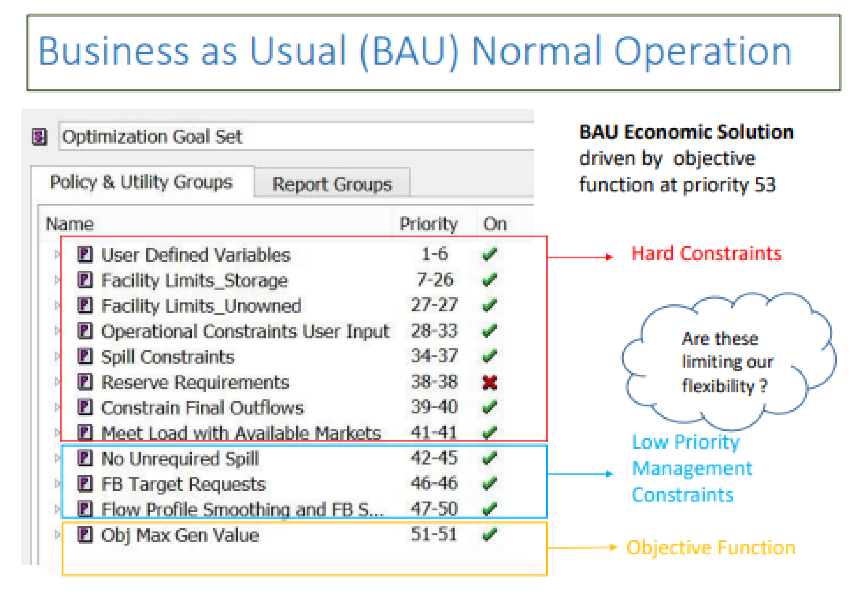
A river and reservoir system model with realistic operational policies is developed in RiverWare, a general river and reservoir multi-objective modeling software [28,29]. RiverWare’s simulation and optimization capabilities are used in this study to implement the complex reservoir operating decisions associated with both power and non-power policies. RiverWare’s Preemptive Linear Goal Programming Optimization solver [30] is used to determine the optimal allocation of water based on the prioritized goals. In this, a linear program is solved at each priority either to maximize or minimize an explicit objective function or to maximize the satisfaction of a set of soft constraints at that priority. The solver optimizes each goal in order, starting with the highest priority. Before moving to the next lower priority goal, it “freezes” the optimal value of the objective function, implicitly constraining lower priority goals to meet the optimal values of higher priority goals so that lower priority goals cannot degrade it. The solver finds the solution within the remaining solution space after the higher priority goals have been optimized. RiverWare’s optimization solves the entire model—all objects and decision variables and for all timesteps simultaneously, finding the optimal solution considering tradeoffs in time. The algorithm is explained in more detail in Eschenbach et al. [30]. The specific formulation for this problem is presented in Appendix A.
The hydro system modeled in our study is largely motivated by the authors’ experience with modeling in the Columbia River Basin, which is a complex system with many flexibility issues. However, the modeled system has been reduced to five reservoirs in series by combining characteristics of some reservoirs, and some of the policy has been streamlined to be less intricate but have similar effects on flexibility. This simplification allows us to produce fairly realistic results without an extended explanation of model detail and without making a case for sensitive policy changes to real systems. The hydro system is modeled by RiverWare “objects” that represent reservoirs, river reaches and confluences and are linked together to form a network. The physical and hydrologic characteristics of the system are expressed in the model with data and physical process methods; reservoir spill, turbine release, storage, elevation, power generation and other factors are modeled in detail. The lag times, or travel times of the reaches between reservoirs, are also inputs. Other input data to the model are hydrologic data—the inflows into the system at the headwater and confluence points.
Figure 1 shows the reservoirs and river reaches in the model of our system. We briefly summarize the attributes of the five reservoirs from upstream to downstream with names that connote one of the important features of each reservoir: Large Reservoir, Unowned Reservoir, Small Reservoir, Reregulating Reservoir and Environmental Reservoir. Large Reservoir has a sizable storage and receives inflows from the upstream systems and contributes a large portion of the system generation. It has a forebay target constraint that sets its pool elevation to some desirable operating level. Unowned Reservoir represents an unowned project with one or more reservoirs which are managed by a reservoir operator(s) different from the one that is managing the rest of the projects in this system. The unowned project is modeled as a storage reservoir with limited storage, and its generation does not count towards system generation in our model because it is part of a different system. Only the release from the Unowned Reservoir is of interest because it passes into the next reservoir in the series of our modeled system. Small Reservoir has small storage with limited turbine capacity leading to frequent spill. Reregulating Reservoir serves a buffering function to partially modulate both upstream and downstream needs and the most downstream reservoir, Environmental Reservoir, that has significant environmental flow constraints. The lag times between these reservoirs are, respectively, 8, 11, 3 and 11 h.
The characteristics of the reservoirs and their hydro plants are shown in Table 1.
2.3. Business as Usual Operation
The Business as Usual (BAU) operation is the normal, or baseline, operation against which changes will be made to test the possibility of increasing flexibility. The BAU policy consists of constraints that can be classified into high-priority constraints and low-priority management constraints as described in Section 2.1. The complete policy is included in Appendix A.
2.3.1. High-Priority Constraints
The high-priority constraints are critical to the operation of the system and are not violated in this study; they ascertain that the minimum and maximum reservoir storage and hydro capacities are never violated and that flow variables such as turbine release, spill, tailwater drawdown, pool elevation, etc. remain within some desirable range that is governed by the seasonal hydrologic conditions.
- Spill for fish passage: a high-priority spill constraint ensures that the regulated spill required for the fish passage operation is always available.
- End of run storage and outflows: to keep the optimization solution from draining the reservoirs to maximize generation, there are constraints that set the final outflows and storage at the end of run period equal to some specified values.
- Energy marketing transactions: to ensure that the system is meeting load at all times, marketing transactions in hourly sales and purchases of energy are carried out during surplus and deficit, respectively.
All of these high-priority constraints are included in all of the study runs—BAU and all other test cases.
2.3.2. Low-Priority Constraints
The low-priority management constraints, in general, conform to traditional standard reservoir operating rules as discussed in Section 2.1. This system’s BAU policy includes these low priority constraints:
- No voluntary spill: this constraint is a common operational policy that reflects the view that it is always better to release water through the turbines and generate some energy, than to “waste” it through the spillways.
- Forebay targets—daily or 7-day: reservoir storage for power generation typically operates within an elevation range, but either daily or 7-day Forebay (FB) targets are often imposed to limit this range by forcing the reservoirs to follow an elevation sequence over time that does not have specific operational benefits.
- Smoothing: “solution quality” constraints lead to smoother operations that are often considered more acceptable by operators. These constraints include flow profile smoothing and maintaining stable Forebay (FB) elevations.
The formulations of the constraints are detailed in Appendix A.
System reserves are typically used to address the uncertainties associated with variable renewable integration and respond to load variations. Since this objective also affects flexibility, the existing policies in BAU operation are developed without a reserve constraint.
2.3.3. BAU Operating Objectives
The hydro system is operated with two main power objectives: meeting the system load and generating revenue from the sale of surplus power. To this end, the system participates in the power market in such a way that it is able to meet its power obligation in all conditions while maximizing the total net economic value of generation from the sale of surplus power and purchase of power at low cost. The numbers of purchases and sales are limited to 5000 MW in the study; this reflects typical market limits because of transmission capacity.
In this study, the BAU optimization is an economic optimization since its objective function determines the quantity and timing of releases from each reservoir subject to the BAU constraints by maximizing the total economic value of generation over the forecast period. The BAU objective function and solution are, respectively, called economic objective and economic solution. The economic value of generation depends on the hourly system generation, hourly energy sales and purchases and the respective energy prices.
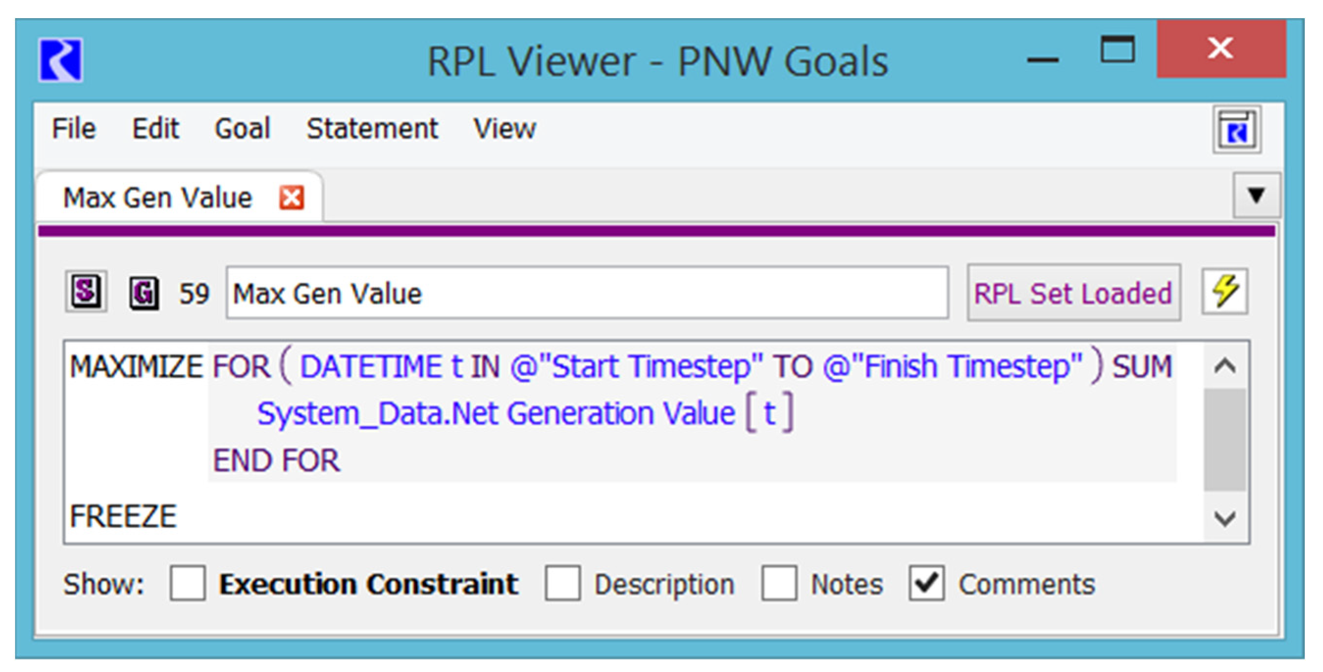
The formulation of the economic objective is detailed in Appendix A.
2.4. Analysis Periods and Data
To understand how flexibility is affected differently in different seasons, the analysis considers two separate 11-day periods, one in April and one in September. The 11-day period considers model performance, availability of experimental data and the goal to quantify the effects of the 7-day forebay target constraint on flexibility. This period also considers flexibility over different days of the week and how later days are affected by deploying flexibility on any of the first seven days of the period.
The model is furnished with unique hourly time series of hydrologic data for each season. These seasons differ in hydrologic conditions, load obligation and constraints. The limits within which the reservoirs can operate also vary between the seasons due to the seasonal hydrologic conditions. In addition, the spill requirement for the fish passage operation is quite high in April and negligible in September. The analyses were carried out for six different seasons, but the results for these two seasons capture the notable differences.
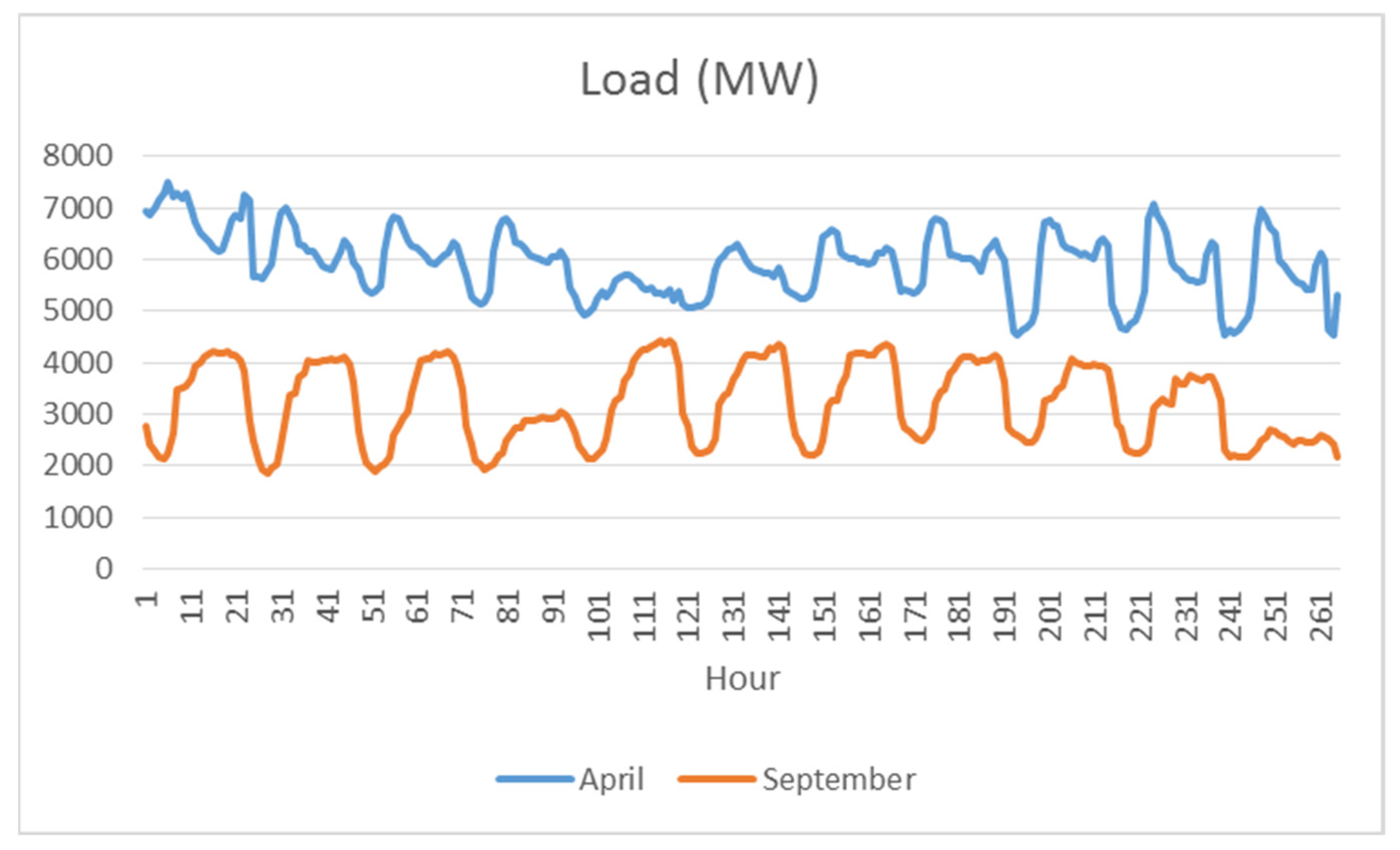
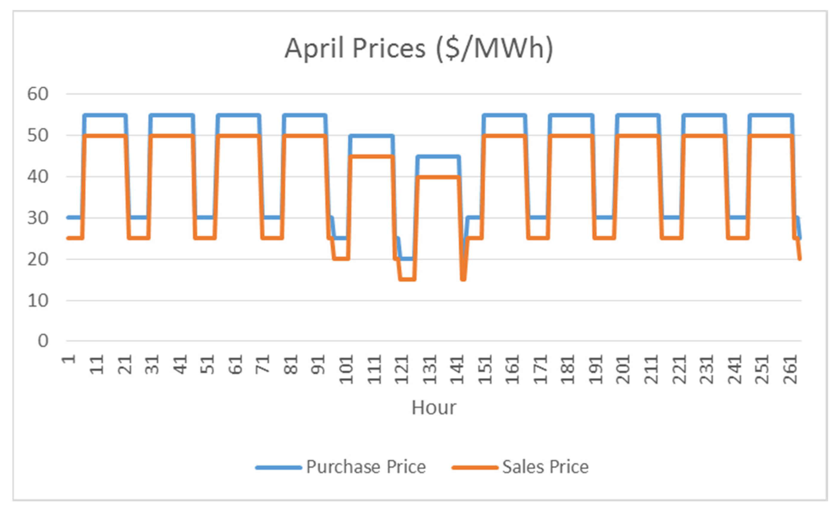
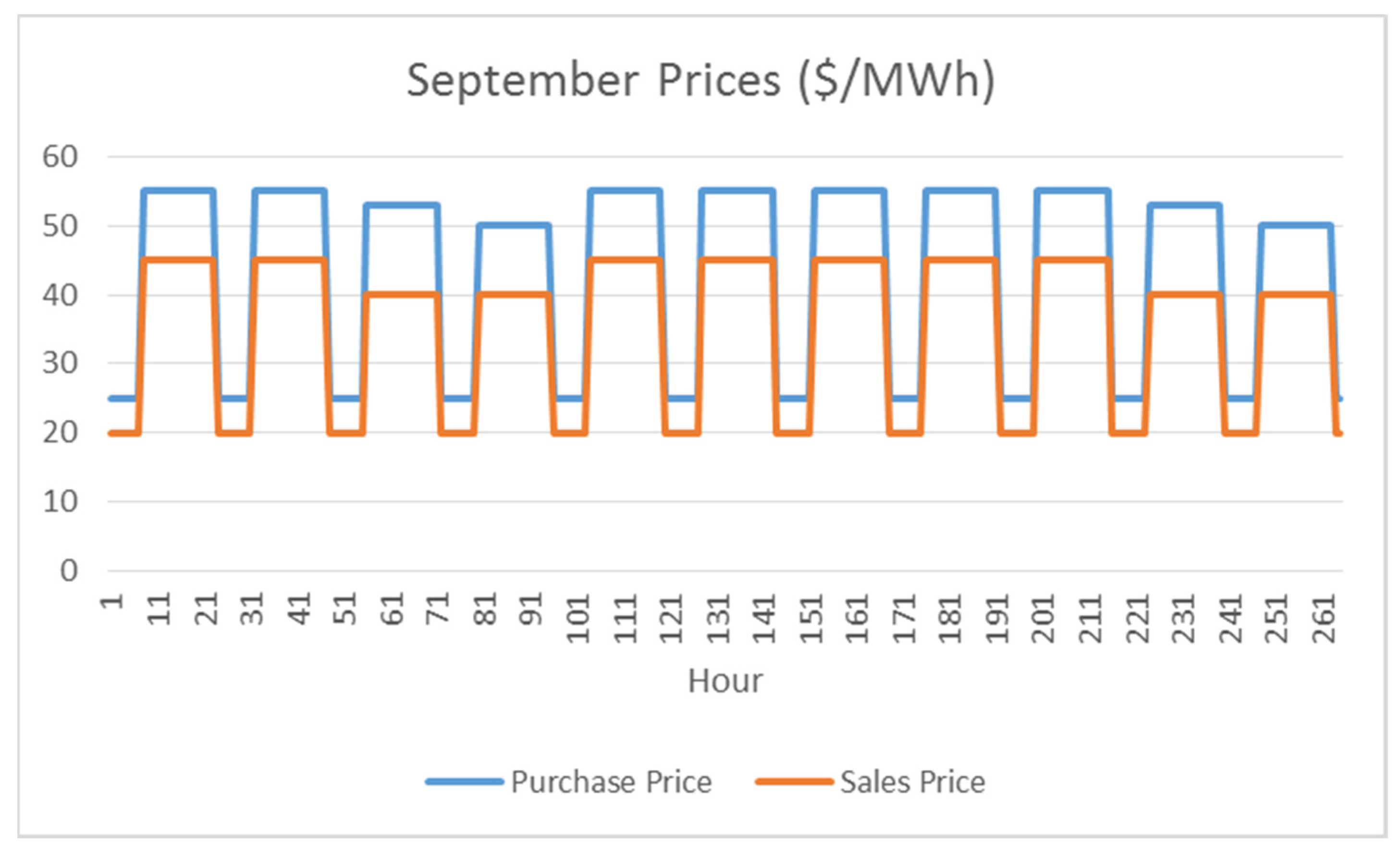
The energy prices in each season depend on the local load with higher price during higher demand. The hourly load demand in April is quite high compared to September. Figure 2 shows the load for both seasons. Figure 3 and Figure 4 show the April and September prices, respectively. All of the figures exhibit daily peaking patterns.
2.5. Flexibility Computations
Given the BAU schedule and economic solution for 11 days, flexibility for a single day is the amount that the generation can be increased or decreased for that day. Upward flexibility—increasing power generation—is possible only during peak load hours, and downward flexibility—decreasing generation—only during nadir hours because upward flexibility is generally not challenging for a hydropower system during off-peak hours and downward flexibility is not difficult during off-nadir hours. To evaluate the flexibility in either the upward or downward direction, a new objective function is introduced at a priority higher than the BAU economic objective that drives the optimization solution, after all the higher priority constraints have been met as well as possible, by either maximizing the total on-peak generation in the upward direction or minimizing the total nadir generation in the downward direction for a single day. The solver then freezes this maximal flexibility. The days prior to the day evaluated are constrained to follow the initial economic solution. Subsequent days would have a new economic solution within the remaining solution space for the day being evaluated and the remaining days.
The solutions of the reformulated flexibility optimization in the respective directions are called the up-flexible solution and the down-flexible solution. The upward flexibility is the increase in energy generated during the peak hours by the up-flexible solution relative to the economic solution. Conversely, the downward flexibility is the decrease in energy generated during the nadir hours by the down-flexible solution relative to the economic solution. Data indicated peak load hours from 8 a.m. to 12 p.m. and nadir load hours from 12 a.m. to 3 a.m. in both seasons. Figure 5 shows the optimization formulation for a single day, called the FlexDay. RiverWare’s optimizer solves the generation for the 11 days in a single optimization solution with the constraints, goals and objectives indicated for the different days as shown. For each optimization, the solution finds either the maximum upward flex or the maximum downward flex. Both solutions are calculated for each FlexDay.
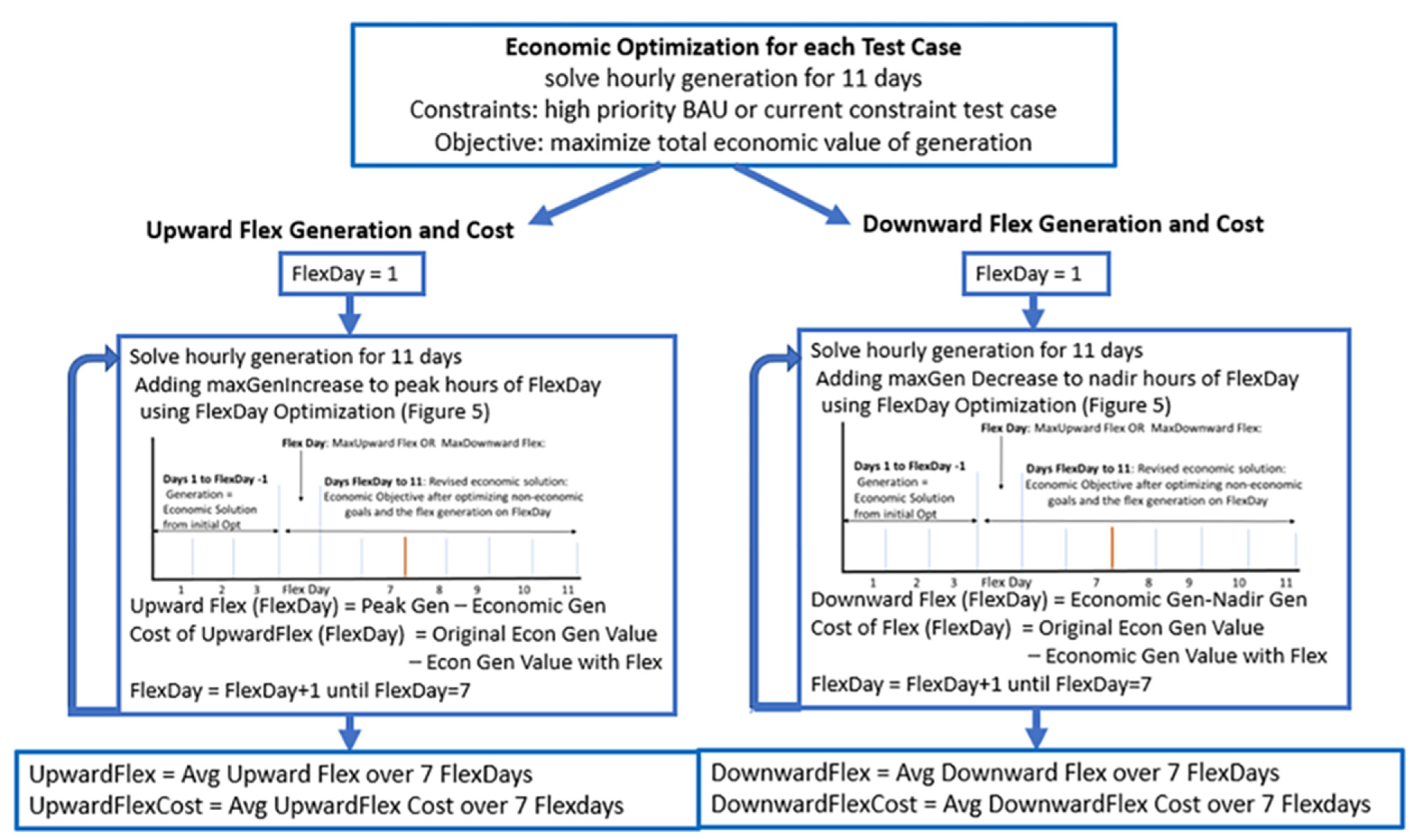
To increase the sample size and cover different days of the week, we reran the optimization with each of the first seven days being the FlexDay evaluated for flexibility in both upward and downward directions. The magnitudes of flexibility and the value (or cost) of the flexibility thus obtained in each of the seven days are averaged to obtain a single quantifiable measure of flexibility and its cost in either direction, and the associated variability is measured by the standard error. Figure 6 shows the steps for computing the average UpFlex and DownFlex generations and values for the 7 flex days.
In addition to quantifying the available flexibility, this study also addresses two important considerations in flexibility evaluation: the limitations imposed by the power market on fully utilizing the available flexibility for a given day and the ability of the later days to adjust their generation as a result of utilizing the technically available flexibility. To address the former consideration, it is assumed that the system participates in the increasingly common practice of day-ahead power marketing [31]. In this power market, the hourly energy sales and purchases for any operating day are committed to the market a day in advance, and these transactions are determined by the economic optimization. The flexibility evaluated on any operating day should, therefore, preserve the economic solutions during the prior days while allowing only the peak or nadir load hours to change during the day being studied for flexibility. The latter consideration is addressed by allowing the later days to change their economic solutions due to flexible operation on the day being studied for flexibility. These changes in later days are included in the total economic value of generation. The flexibility evaluated on each day should incorporate both adjustments: the day exercising flexibility and the later days reacting to those changes.
2.6. Flexibility Experiments
The flexibility experiments were designed as variations in the BAU to quantify how flexibility is affected by (1) various low-priority management constraints; (2) lags in hydraulic travel time between power plants; (3) maintaining operating reserves for variable renewables; and (4) managing the system with unknown releases from the Unowned Reservoir in the middle of the managed system. The flexibility for each system setting is compared with the baseline system setting. The baseline system has many low-priority constraints, has lags present between the adjacent reservoirs, the operating reserves obligation is not imposed and the release from the Unowned Reservoir is approximated as passing inflows. For each system setting, the flexibility due to different variations in the policies present in BAU operation are compared against the flexibility due to the respective policies’ variations in the baseline system. An important example is the policy having to do with constraining forebay elevations; target forebay elevations from a longer time horizon model are often used to constrain, and possibly over-constrain [32], shorter time horizon models. We include the significant effect of forebay targets on maximizing flexibility. The constraints are explained in detail below.
2.6.1. Effects of Low-Priority Constraints
To compare cases of heavily constrained or more relaxed systems, and to identify effects of specific low-priority constraints, different variations of policies from the existing BAU policies are built.
BAU—high-priority constraints including operational spill for fish passage and keeping variables in required ranges; 3 low-priority constraints—no voluntary spill, 7-day forebay target and solution quality constraints.
- C0—minimal constraints, includes all the high-priority constraints described in BAU but no low-priority constraints;
- C1—C0 constraints and one additional constraint, no voluntary spill; this allows required spills but does not allow the reservoir to spill more water than what is required;
- C2—C1 constraints and one additional constraint, an end of 7-day FB target. This constrains the pool elevation to maintain some prescribed elevation at the end of day 7 (a forebay target);
- C3 (constraints in BAU)—this constraint level has all the constraints present in C2 and additional solution quality constraints. These constraints include flow profile smoothing constraints that control the spikes in outflows and an FB stable constraint that prevents the reservoir’s pool elevation from fluctuating rapidly between two consecutive time steps.
The list of low-priority constraints in each constraint level is shown in Table 2.
It should be noted that the economic optimization, in many cases, improves in both upward and downward directions in a more relaxed system. This improvement might limit the available flexibility in either direction as the economic solution absorbs most of the additional generation capability. Therefore, to retain the magnitudes of flexibility in less constrained levels that are potentially absorbed by their economic solutions, the maximum or minimum generation capabilities for constraint levels C0, C1 and C2 are compared against the economic solution for the constrained case C3.
To study the effects of different target FB frequencies on flexibility, two additional constraint alternatives are:
- FB7—has only the high-priority constraints present in C0 and one additional constraint end of 7-day FB target;
- FBDaily—has only the high-priority constraints present in C0 and one additional constraint daily FB target, which constrains the pool elevation to some prescribed elevation at the end of each day.
2.6.2. Effects of System Factors
It is worth exploring and understanding how certain river and reservoir system characteristics and modeling assumptions affect the hydro system operation and consequently limit or increase its flexibility. The system factors included in this study are the following.
- No-Lag Case: the baseline system has considerable travel time lags between adjacent reservoirs. To quantify the impact of these lags on flexibility, the flexibility is assessed in an alternative model with no lags.
- Operating Reserve Case: the integration of renewable resources in a hydro system forces the system to maintain sufficient down and up reserves to respond to uncertainties associated with their variable generation. Some systems also hold these reserves to respond to load variations. This type of dedicated reserve for uncertain generation is analogous to allocating reservoir storage space for flood control or other reservoir uses for inflow uncertainty. These kinds of reserve obligations could limit flexibility for other forms of variability such as hydrologic uncertainty and market price fluctuations. The BAU policies are modified to introduce additional limitations on the flow variables due to system reserve requirements in both up and down directions. Reserves were chosen to be comparable to reserves used in the Columbia River Basin.
- Load Shaping for the Unowned Reservoir: the unknown release from the Unowned Reservoir is modeled in the baseline system by passing inflows, a simple and easy to implement model the authors have seen in practice. Passing inflows do not allow the initial storage in this project to change during the entire run period. The alternative system modeling for the flexibility assessment assumes load shaping of unknown release with the assumption that the Unowned Reservoir faces a similar load profile, but passes total inflow over the course of each day while using available storage during the day for peaking. With a load shaping profile, the Unowned Reservoir will be somewhat in sync with the owned reservoirs. The flexibility obtained for this system setting is compared with the no-lag system rather than the usual baseline because the load shaping effects might not be apparent when there are considerable lags in the system. Certainly, more precise and more complex models of the Unowned Reservoir can be made.
All of the experiments including those for system factors evaluated and their respective baseline and test systems are shown in Table 3.
The flexibility for each system setting is evaluated for all the constraint levels discussed in Section 2.6.1. For a particular system setting, the flexibility for each constraint level is measured relative to the BAU economic generation in C3.
However, it is not possible to directly compare the flexibility between the test (alternate) system and the existing (baseline) system because the BAU economic generation, relative to which the flexibility is measured, is not the same for these systems. The economic generation for one system setting might provide or take up some of the available flexibility relative to another system setting. For example, one would expect removing lag times to cause an increase in economic generation on-peak because inflows downstream are arriving exactly when they are needed for generation. The ability to have additional upward flexibility beyond the economic generation remains a question to be tested with our experiments.
2.6.3. Effect of Deploying Flexibility
Suppose the available flexibility were fully deployed on the day evaluated, what is the effect on economic generation in later days? No additional experiments are needed to answer this question. We need only collect this information during the experiment and compare it to the generation for these days without a flexibility objective.
3. Results
The raw results have values for each of the first seven days that were separately evaluated as the “flexibility day”. To simplify the presentation, we largely refer to the mean values across the seven days. The plots in this section also show the standard errors.
3.1. Effects of Business as Usual (BAU) Low-Priority Management Constraints on Flexibility
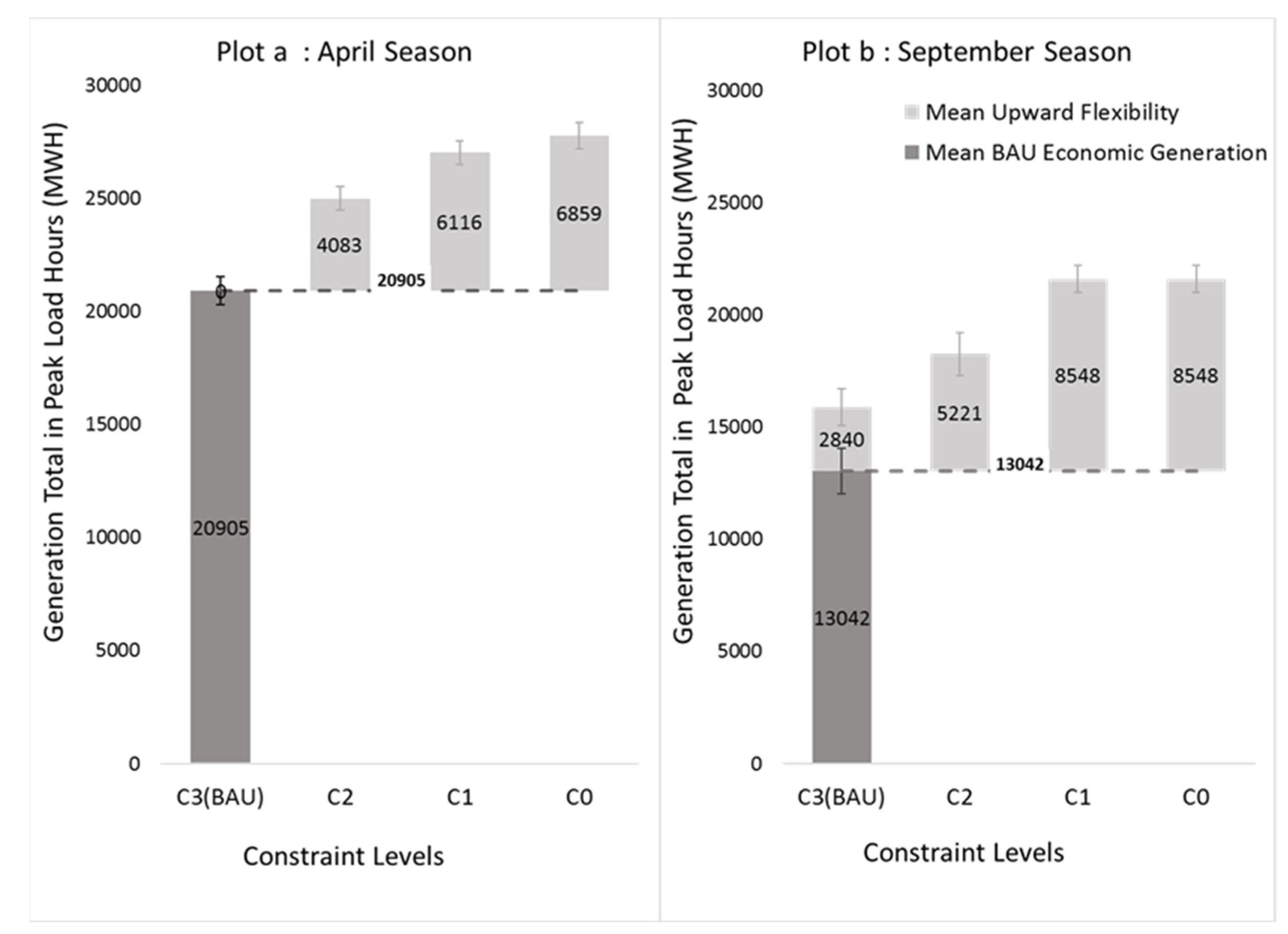
For the baseline system (non-zero lag times, no dedicated reserves and passing inflows at the Unowned Reservoir), the mean upward flexibilities for the constraint levels C3 through C0 are shown in Figure 7 for the two seasons, April and September. Moving from left to right in each plot, the constraint levels represent a transition from the highly constrained BAU system, C3, to the most relaxed system C0 having no low-priority management constraints. The list of low-priority constraints present in each constraint level was shown earlier in Table 2.
As is evident from the plots in Figure 7, successively removing the low-priority management constraints from C3 results in an increase in upward flexibility. In April, there is no upward flexibility after all the BAU constraints are applied. Removing the smoothing constraints, C2, provides an average of more than 4083 MWH of potential increased generation at peak load hours. This is ~20% more than the generation that is most economically produced without consideration of flexibility. Without the 7-day forebay target, C1, more than 2033 MWH of additional flexibility is gained, and dropping the no-spill constraint in C0, the minimally constrained level, provides another 743 MWH on average during the peak hours. In September, there are 2840 MWH of potential additional energy over the BAU best economic solution with the C3 constraints. This is ~21% more generation than the most economically produced BAU generation. Dropping the smoothing constraints brings this to 5221 MWH in C2. Further dropping the 7-day forebay constraint with C1 again greatly increases the upward flexibility. However, the no-spill constraint has no effect in September.
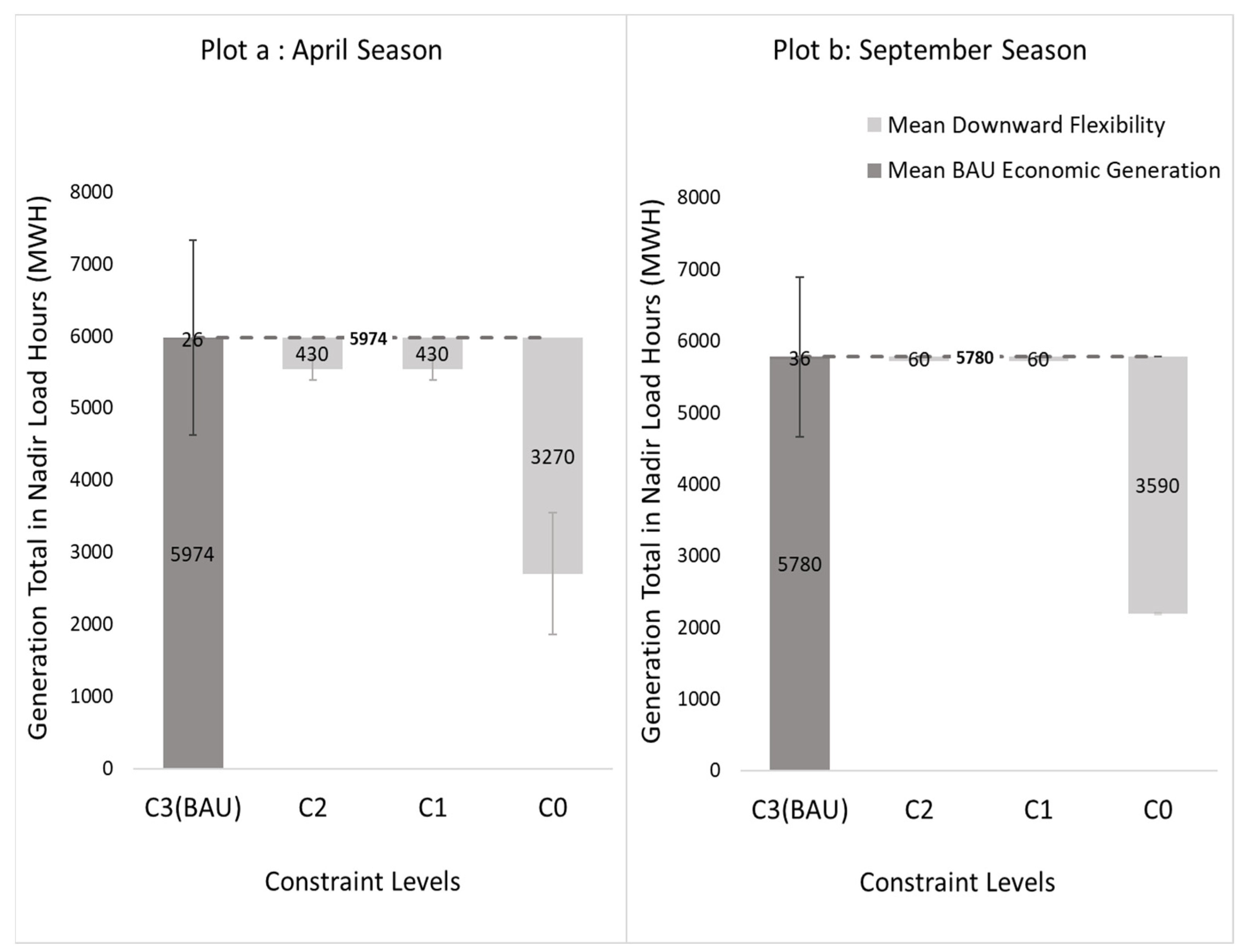
Similarly, the plots in Figure 8 show that in April, downward flexibility increases only slightly for C2, with no further gain for C1. In September, neither C2 nor C1 shows any notable downward flexibility gains. However, in both seasons, removing the no-spill constraint with C0 provides large downward flexibility with potential reduction of the BAU economic generation by 55% in April and 62% in September.
3.2. Effect of Forebay Target Frequency
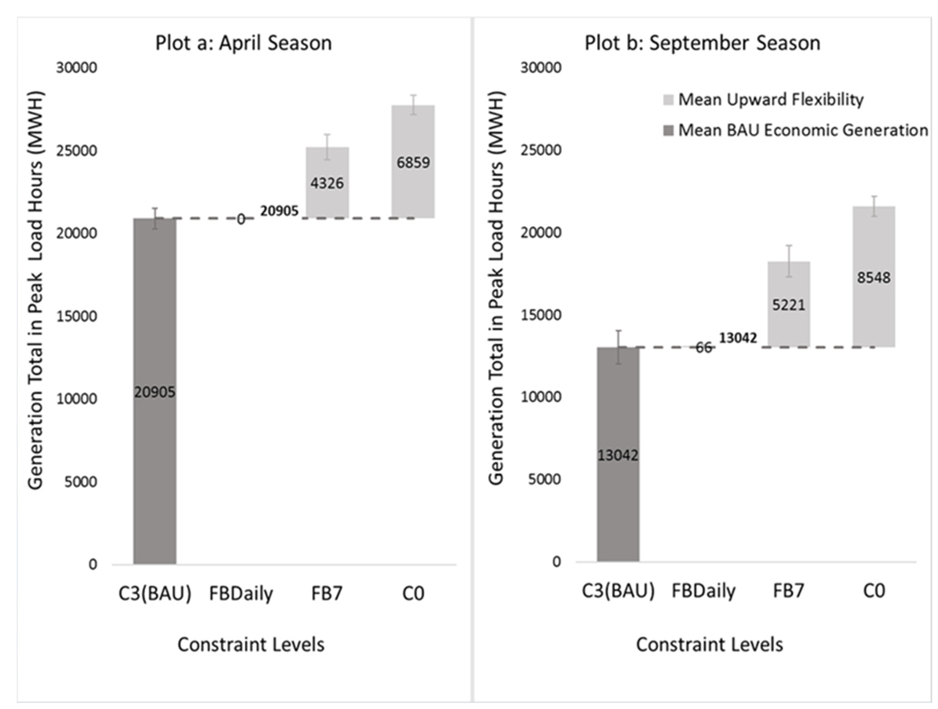
Two constraint levels, FBDaily with daily forebay targets, and FB7 with an end of 7-day forebay target, added to the minimally constrained level C0, were defined in Section 2.6.1. The magnitudes of upward flexibility due to all three constraint levels are presented in Figure 9. The flexibility for each constraint level is measured relative to the mean total BAU economic generation at peak load hours due to constraint level C3. The magnitudes of the BAU economic generations for April and September are shown by the left-most vertical bars in the respective plots. Since the more constrained BAU operation or C3 level has “no voluntary spill” and “solution quality” constraints in addition to an end of 7-day target constraint, the magnitudes of flexibility for the BAU operation are not included in the plots to highlight the impacts of forebay target frequency on the flexibility alone.
As seen in Figure 9, decreasing the forebay target frequency from daily to only day 7 greatly increases the upward flexibility. With the daily forebay target active, in April, there is no upward flexibility available relative to the BAU economic generation, and only 66 MWH in September. With a day 7 only forebay target, the available flexibility increases in April to 20% greater than the BAU economic generation, and to 40% greater in September. With no target elevations active in the operating policy, C0, the respective available flexibilities in April and September are 32% and 65%, respectively, of the BAU economic generation. A similar comparison of downward flexibility for C0, FBDaily and FB7 finds that the forebay target frequency does not have any effect on downward flexibility in our test model.
3.3. Effect of System Factors
As described in Section 2.6, the impacts of several system factors on flexibility are quantified by an alternative modeling of the existing system. However, as described, it is not possible to directly compare the available flexibility between the test (alternate) system and the existing (baseline) system since the BAU economic generation, relative to which the flexibility is measured, is not the same for these two systems. Instead, for upward flexibility, a comparison is made of the total maximum generation for the peak load hours obtained by adding the available upward flexibility to the BAU economic generation. In addition to our flexibility metrics measuring the differences in generation between flexibility solutions and economic solutions, we must also examine the total generation for the peak and nadir hours.
For downward flexibility, a comparison is made of the total minimum generation at nadir load hours, obtained by subtracting the available downward flexibility from the BAU economic generation. The results for each of the system factors—effects of no lags, reserves for variable renewables and assumptions about release from non-owned reservoirs—are presented by comparing the flexibility of the alternate system for all the defined constraint levels against the BAU economic generation at C3, as well as by comparing its generation against the baseline. The BAU economic generations averaged across April and September seasons for the baseline system and different test systems are shown in Table 5. For each test system, flexibility is evaluated for different constraint levels defined in Table 2 and the results are shown in Table 6 as a percentage of the BAU economic generation for the respective system.
3.3.1. Effects of No Lags
Averaging across the seasons, the system with no lags had increased economic generation of 5% (891 MWH) in the peak hours and 2% (120 MWH) in the nadir hours compared to the lagged case. The explanation for these results is that less storage space is required to buffer flows arriving at less valuable times; the peaking flows move through the whole system quickly. One might expect even larger changes in peak generation, but both high- and low-priority constraints still limit the system. The 2% increase in generation during the nadir hours was unexpected, but 120 MWH is relatively insignificant in a system that generates over 20 GW on-peak. One possible explanation is structural limits on ramping down generation can force off-peak generation.
The maximal generation during peaking hours under the C0 case without the low-priority constraints is almost identical in the lag and zero-lag cases, with a 9 MW difference. Thus, the increased economic generation is directly reducing the capability for upward flexibility by 12% compared to the lag case.
The overall pattern of constraints limiting upward flexibility is largely similar in the two cases as shown in Table 6. The BAU case has 8% flexibility for the lag and no-lag cases. Removing smoothing constraints adds 19% and 9%, respectively, and accounts for most of the overall change in flexibility. Removing 7-day forebay constraints adds 16% and 18%, respectively. Removing no-spill constraints adds 2% and 3%, respectively.
The overall pattern of constraints limiting downward flexibility is largely similar in the two cases. The minimal generation during nadir hours in the C0 case differs by only 41 MWH between the lag and zero-lag cases. The BAU case has 1% of the downward flexibility of the C0 case for both the lag and zero lag cases. Removing the smoothing and 7-day forebay constraints adds 6% of the flexibility of the C0 case and removing the no-spill constraints adds 93% of the flexibility for both the lag and zero-lag cases.
3.3.2. Effect of Reserves
The reserve requirements for a hydro system with variable renewable integration vary seasonally due to differences in hydrologic conditions, load obligations and operational needs. To address this, the BAU policies, which do not include reserves, are modified to include the hourly up and down reserve requirements for both April and September seasons. For April, these are set to 800 MW and 500 MW, respectively, and in September to 1000 MW and 800 MW, respectively. Since the peak and nadir hours in our flexibility experiments are four and three hours in duration, respectively, total up reserves and down reserves held during the respective periods in April are 3200 MWH and 1500 MWH, and in September these are 4000 MWH and 2400 MWH. These values are sufficient to address the uncertainties associated with the variable renewable integration and respond to the load variations in each season for our hydro system model. The economic generation in any system with operating reserve requirements such as this depends on the magnitudes of up reserves and down reserves held and their resulting net effect. As a result of holding these reserves, the economic value of generation decreases by 25% in September because of lower peak generation and increases by 22% in April because of increased off-peak generation compared to the system without reserves. The constraints in this system affect the flexibility in a similar manner to the baseline and no-lag systems but the magnitudes of their impacts on the upward flexibility are less in this system compared to both baseline and no-lag systems, as shown in Table 5:
- the largest increases in upward flexibility are realized by removing the 7-day FB target and smoothing constraints;
- the largest increases in downward flexibility are realized by removing the no-spill constraint.
The reason that the results follow a similar pattern with reduced flexibility is that the reserves have used some of the flexibility.
We examine this reduction in more depth for the C0 case which has the largest flexibility change of the constraint cases when reserves are used. The magnitudes of mean upward flexibility at C0 during peak hours in April and September decrease, respectively, by 3227 MWH and 3483 MWH when the up reserves equivalent to 3200 MWH and 4000 MWH are held in each season, respectively. Similarly, the magnitudes of mean downward flexibility at C0 during nadir hours in April and September decrease, respectively, by 982 MWH and 2309 MWH when down reserves of 1500 MWH and 2400 MWH are held in each season, respectively. Thus, the reserves cut into the flexibility for the C0 case. The loss in flexibility by holding reserves is less than the total amount of generation held as reserves for the September upward flexibility and April downward flexibility. In contrast, the April upward flexibility and the September downward flexibility have close to a one for one tradeoff. An argument can be made for combining upward flexibility and reserves and also downward flexibility and reserves. The result is the decrease in net upward total generation by 27 MWH in April and its increase by 517 MWH in September. Similarly, the net downward total decreases by 518 MWH and 91 MWH, respectively. These results are also true for constraint levels C1, C2 and FB7.
3.3.3. Effect of Load-Shaping Assumption for Release from Unowned Reservoir
To evaluate the effects of assuming a load-shaping release from the Unowned Reservoir rather than simply passing inflows, we use as a baseline the no-lag system. The effect of assuming load shaping for unowned projects essentially magnifies the effect of removing lags from the baseline system model. The mean BAU economic generation in the peak period with this system setting increases by 5% in April and 14% in September when compared against the no-lag system. Similarly, the generation during the nadir period decreases by 28% in April and 48% in September. The economic value of generation improves dramatically: 28% in April and 88% in September. The explanation is that the load following release pattern is closer to the economic release pattern of the upstream and downstream reservoirs, and with no lag the water passes through the system quickly.
However, these economic improvements in generation reduce the availability of flexibility in this system. Averaging across the seasons, removing the solution quality constraints from the BAU constraints contributes to 4% more upward flexibility in C2. The removal of the 7-day forebay target results in 17% more upward flexibility. Further removing the no-spill constraint results in 5% more flexibility. Removing the solution quality and forebay target constraints mildly increases downward flexibility by 4% but removing the no-spill constraint increases downward flexibility by 35%. The baseline no-lag case that passes inflows has a larger percentage equal to 59%. Thus, we can conclude that both removing lags and assuming unowned reservoirs follow load shaping instead of passing inflows have the effects of improving economic solutions that use up the potential for both upward and downward flexibility.
3.4. Economic Effect of Deploying Flexibility
Figure 10 depicts how using the technically available upward flexibility on any particular day decreases the economic generation in later days. The use of flexibility during the peak load hours on day 4 results in an average of −32 MW loss of economic generation in later days. The generation changes in these hours are due to changes in the reservoirs’ storage levels after using the available flexibility on day 4.
The cost of upward flexibility is directly related to this loss of generation and is shown in Figure 11. Figure 11 also shows the result of a linear regression on this data for all seven days. The regression is a good fit with an R2 value of 0.9909. The rate of increase in cost or rate of loss of economic value of generation per unit change in upward flexibility is 50 $/MWh of used flexibility. This value is similar to the peak value of sales and purchases shown in Figure 4. While this cost may be higher than the average generation value, it may be reasonable compared to the consequences of not having enough flexibility in the system when needed. The cost of using the available flexibility could be quite different in another system.
This relationship is also true for the April season although the R2 value is slightly less. There is negligible cost to flexibility when the magnitude of flexibility is close to 0 and no apparent relationship between cost and flexibility exists for constraint levels C0 and C1.
The cost of utilizing downward flexibility is different: the later days do not change much as a consequence of utilizing the downward flexibility. The reason is that downward flexibility comes largely from spilling and it does not change the reservoirs’ storage levels in later days. Consequently, utilizing it does not affect the generation in these later hours, and the only cost associated with deploying downward flexibility is the cost of spilling or the cost of foregone generation.
4. Discussion
Upward flexibility is strongly affected by low-priority policies such as smoothing constraints and 7-day forebay targets with similar magnitudes of impact for each. However, no-spill constraints had little to no effect on upward flexibility. Increasing the frequency of forebay targets from seven days to daily eliminates almost all flexibility. This overall pattern, but not the magnitude of flexibility, held true regardless of experiments with different assumptions: different seasons, zero lag time between reservoirs, different assumptions about the operation of unowned reservoirs and holding dedicated reserves. High-flow seasons, zero lags and unowned reservoirs with generation following load all resulted in an increased baseline economic generation during peak hours which resulted in a smaller ability for upward flexibility during peak hours. Dedicated reserves reduced both economic generation and the flexibility beyond the reserves. In some cases, reserves replaced flexibility at almost a one for one rate, but in other cases the reduction in flexibility was smaller.
Only downward flexibility during nadir hours was substantially affected by no-spill constraints. Other low-priority constraints and all of the other experimental variations had only minimal effects. Thus, a reasonable approximation would be to ignore these effects and concentrate on the ability of reservoirs to spill and the lost opportunity cost of spilled energy. In this sense, downward flexibility is almost a separate question from upward flexibility.
There are two primary costs associated with flexibility, the deployment cost and the opportunity cost. The deployment cost of upward flexibility is a shift in the timing of generation. In this study, we found the cost was directly proportional to the flexibility deployed with a value of $50/MWH, but we would expect the value for hydropower operators to be strongly related to regional prices and seasonality. The deployment cost of downward flexibility is largely due to voluntary spill: the cost of lost future generation and, if the gates are manually operated, the cost of gate changes.
Dedicated hydropower reserves are sometimes considered a panacea for absorbing the variable generation produced by ever increasing renewable penetration. While using hydropower this way is clearly useful, it does come with an opportunity cost. In this study, we found that the level of reserves resulted in substantial opportunity costs, 22–25% reduction in the economic value of hydropower generation and significant reduction in the amount of flexibility available for other purposes.
There are several opportunities for future study and operational changes suggested by this research: more careful consideration of low-priority constraints and their impact on flexibility and the modeling of reservoirs owned by others.
Forebay levels capture most of the state of a reservoir system, and forebay targets are a common way to constrain shorter timestep models based on the outcome of larger timestep models. This research suggests some caution in using these targets, particularly as the time until the target becomes shorter. A little flexibility in either the value of the target or delaying the time to meet these targets may dramatically improve upward flexibility. Experimentation with these approaches seems warranted. The vast difference in flexibility impact between daily and weekly forebay targets suggests further research into forebay target frequencies ranging from daily to monthly.
Smooth operations are often prudent and always appealing, but given the impact on upward flexibility, careful consideration should be given to the marginal benefit of smoothing policies compared to the marginal cost in lost flexibility. We suspect that this may be a basin-specific question, but also one that should be considered before either regulators or operators impose smoothing constraints on a system.
Disallowing voluntary spill is often taken to be an obvious part of an optimal reservoir operation strategy because of the lost energy and gate change costs. However, in the context of a larger energy system with cycling of thermal plants or even at a grid level, this spill and investing in automated gates for quick response may be justified by the increase in downward flexibility.
Finally, modeling assumptions about unowned reservoirs have a significant impact on both economic generation and flexibility for the larger system. The results suggest the system effects of even a comparatively small unowned reservoir may make it worthwhile to build more accurate models of how unowned reservoir outflows respond to inflows and other factors. Such a study may also suggest going beyond more accurate modeling and engaging in some degree of mutually beneficial communication or coordination of operations.
5. Conclusions
The main contribution of this research is to identify and quantify the effects of different reservoir system attributes on hydropower flexibility. These attributes include various operating policies, the need to hold reserves, lag times and the presence of reservoirs controlled by others. This is a new contribution to the information about flexibility in hydro systems and uses a novel approach to find specific, usable results. The experiments with a fictional river basin that is similar in characteristics to basins in the Pacific Northwest United States have led to several conclusions about what does and does not affect upward and downward flexibility in reservoir generation and the costs of reserving and deploying flexibility.
The modeled system in this study can inform understanding and estimates of flexibility in other regions. Although based on reservoirs in the northwest US, the projects are typical of characteristics of river systems throughout the U.S. The distribution of hydro generation in the US ranges from 27% in Washington to 5% in Tennessee, with large contributions from New York, California and Alabama [33]. The largest producing areas have a share of large reservoirs, but all of the most significant hydro-producing river systems have a combination of large and small reservoirs with a variety of multi-purpose uses and hydraulic characteristics. For this study, our projects range from 122 to 6599 Mm3 of storage and from 1.2 to 6.7 MW of generating capacity. Furthermore, of the more than 2000 active hydro plants in the US, only about 2.5% have hydropower as the primary authorized purpose [34], which justifies RiverWare’s approach of multi-objective modeling in which hydropower is considered along with the other purposes of the projects. RiverWare is widely used for modeling multi-objective reservoir operations in the Columbia River Basin, the Tennessee Valley Authority, the Bureau of Reclamation in many of Reclamation’s river systems including the Colorado River Basin, the U.S. Army Corps of Engineers on the Rio Grande, Arkansas and White River Systems, the Southwest Power Administration, the Lower Colorado River Authority and other utilities and water authorities.
There are several opportunities for future study and operational changes suggested by this research: more careful consideration of low-priority constraints and their impact on flexibility and the modeling of reservoirs owned by others. The computations could be reproduced for actual or hypothetical reservoirs with different attributes in other areas. A further study could also confirm the extent to which our results are valid in actual systems in the northwest or in other areas. Other important related topics such as the influence of flexibility on hydraulic machines in hydro plants could expand the usefulness of the research.
Author Contributions
Conceptualization, T.M. and E.Z.; methodology, T.M., S.T. and E.Z.; software, S.T.; validation, S.T., T.M. and E.Z.; formal analysis, S.T.; investigation, S.T. and T.M.; resources, E.Z. and T.M.; data curation, T.M.; writing—original draft preparation, S.T.; writing—review and editing, T.M. and E.Z.; visualization, S.T.; supervision, E.Z. and T.M.; project administration, E.Z.; funding acquisition, E.Z. All authors have read and agreed to the published version of the manuscript.
Funding
This research received no external funding.
Data Availability Statement
Data available on request. RiverWare is a licensed software of the University of Colorado. The software and model files are available from the corresponding author.
Acknowledgments
Senior research staff at CADSWES assisted S.T. with modeling expertise.
Conflicts of Interest
The authors declare no conflict of interest.
Appendix A
The mathematical formulation of the preemptive linear goal program for this study includes the following basic variables and constraints that constitute the basic linear program (LP):
River Reaches
Reservoirs
System
Symbols
Capital letters are used for variables.
t: time index
r: reservoir index
Δt: timestep length
α: power coefficient
S: reservoir storage
QO: outflow
QI: inflow
qh: hydrologic inflow
QS: spill
QT: turbine release
PE: reservoir pool elevation
P: reservoir power
E: reservoir energy
UR: upward reserve power
DR: downward reserve power
maxP: maximum power available
minP: minimum power requirement
EP: energy purchases
ES: energy sales
l: system load
The preemptive goal program adds to the basic LP the goals listed in Figure A1 in priority order. Each goal has a linear or piece-wise linear objective function to either minimize/maximize a function or to minimize violation of soft constraints, using the same set of variables. The exact objective function for minimizing violations varies by goal and either minimizes the sum of violations, squared violations or the largest violations. The linear program for each successive priority is constrained to meet the optimal objective function values for all higher priorities. The highest priority goals such as licensed limits on reservoir operations are typically never violated and are effectively hard constraints. In contrast, lower priority goals such as smoothing constraints are frequently violated because of higher priority goals.
For example, the soft constraints for the low-priority “Minimize Spill Deltas” goal are intended to minimize unnecessary variation in spill and are written
RiverWare automatically translated these to an objective function as follows:
The linear program for all lower priorities is constrained to meet the optimal objective function values for all higher priorities. We refer interested readers to Eschenbach et al. [30] for more detail on the RiverWare formulation of preemptive linear goal programs.
The goal set for the BAU objective is shown in Figure A1 in the RiverWare Goal Set Editor.
Figure A1.
The optimization goals for the BAU economic solution shown in RiverWare’s Goal Set Editor.
Figure A1.
The optimization goals for the BAU economic solution shown in RiverWare’s Goal Set Editor.

For all of the experiments, the high-priority (hard) constraints do not vary. The low-priority constraints are activated or inactivated according to the experiment configurations shown in Table 3. The form of these constraints is as follows:
The BAU economic solution maximizes the value of generation for 11 days:
For the flexibility computation, the following problem is formulated:
Figure A2.
An example of a goal shown in the RiverWare Goal Editor. This is Goal 51, which can be seen in the list of goals in Figure A1.
Figure A2.
An example of a goal shown in the RiverWare Goal Editor. This is Goal 51, which can be seen in the list of goals in Figure A1.

Figure A3.
The palette of operations that is used to construct a goal such as shown in Figure A2.
Figure A3.
The palette of operations that is used to construct a goal such as shown in Figure A2.

References
- Alizadeh, M.I.; Moghaddam, M.P.; Amjady, N.; Siano, P.; Sheikh-El-slami, M.K. Flexibility in future power systems with high renewable penetration: A review. Renew Sustain. Energy Rev. 2016, 57, 1186–1193. [Google Scholar] [CrossRef]
- Oree, V.; Sayed Hassen, S.Z. A composite metric for assessing flexibility available in conventional generators of power systems. Appl. Energy 2016, 177, 683–691. [Google Scholar] [CrossRef]
- Lannoye, E.; Flynn, D.; O’Malley, M. The role of power system flexibility in generation planning. In Proceedings of the IEEE Power and Energy Society General Meeting, Detroit, MI, USA, 24–28 July 2011. [Google Scholar] [CrossRef] [Green Version]
- Ulbig, A. Operational Flexibility in Electric Power systems. Ph.D. Thesis, ETH Zurich, Zurich, Switzerland, 2014. [Google Scholar] [CrossRef]
- Martinez, R.U.; Johnson, M.M.; Shan, R. U.S. Hydropower Market Report (January 2021 Edition). 2021. Available online: https://www.osti.gov/servlets/purl/1763453 (accessed on 24 May 2021).
- Key, T.; Rogers, L.; Brooks, D.; Tuohy, A. Quantifying the Value of Hydropower in the Electric Grid: Final Report; Energy Efficiency and Renewable Energy (EERE): Washington, DC, USA, 2012. [Google Scholar] [CrossRef] [Green Version]
- Khan, N.; Tingsanchali, T. Optimization and simulation of reservoir operation with sediment evacuation: A case study of the Tarbela Dam, Pakistan. Hydr. Proc. 2009, 23, 730–747. [Google Scholar] [CrossRef]
- Stoll, B.; Andrade, J.; Cohen, S.; Brinkman, G.; Brancucci Martinez-Anido, C. Hydropower Modeling Challenges (No. NREL/TP-5D00-68231) 2017; National Renewable Energy Lab (NREL): Golden, CO, USA, 2017. [Google Scholar]
- Oliveira, R.; Loucks, D.P. Operating rules for multireservoir systems. Water Resour. Res. 1997, 33, 839–852. [Google Scholar] [CrossRef]
- Harby, A.; Schäffer, L.E.; Arnesen, F.; Bauhofer, P.; Beckitt, A.; Bockenhauer, S.; Botterud, A.; Christensen, T.H.; Middleton, L.; Nielsen, N.; et al. Flexible Hydropower Providing Value to Renewable Energy Integration. White Paper. IEA Hydropower, Annex IX. 2019. Available online: https://www.ieahydro.org/news/2019/10/iea-hydro-tcp-annex-ix-publishes-white-paper-on-flexible-hydropower-providing (accessed on 23 June 2022).
- Hirth, L. The benefits of flexibility: The value of wind energy with hydropower. Appl. Energy 2016, 181, 210–223. [Google Scholar] [CrossRef]
- Lannoye, E.; Tuohy, A.; Flynn, D.; Daly, P. Assessing power system flexibility for variable renewable integration: A flexibility metric for long-term system planning. CIGRE. Sci. Eng. J. 2015, 3, 26–39. [Google Scholar]
- Clement, M.; Magee, T.; Zagona, E. A Methodology to Assess the Value of Integrated Hydropower and Wind Generation. Wind Eng. 2014, 38, 261–276. [Google Scholar] [CrossRef] [Green Version]
- Ibanez, E.; Magee, T.; Clement, M.; Brinkman, G.; Milligan, M.; Zagona, E. Enhancing Hydropower Modeling in Variable Generation Integration Studies. Energy 2014, 74, 518–528. [Google Scholar] [CrossRef] [Green Version]
- Menemenlis, N.; Huneault, M.; Robitaille, A. Thoughts on power system flexibility quantification for the short-term horizon. In Proceedings of the IEEE Power and Energy Society General Meeting, Detroit, MI, USA, 24–28 July 2011. [Google Scholar] [CrossRef]
- Energy KnowledgeBase. Duck Curve. Available online: https://energyknowledgebase.com/topics/duck-curve.asp (accessed on 23 June 2022).
- California ISO 2016. Available online: https://www.caiso.com/Documents/FlexibleResourcesHelpRenewables_FastFacts.pdf (accessed on 23 June 2022).
- Department of Energy 2021. September 30. DOE Announces $8.5 Million to Increase Hydropower Flexibility. Available online: https://www.energy.gov/eere/articles/doe-announces-85-million-increase-hydropower-flexibility (accessed on 24 June 2022).
- Bashiri, H.; Sharifi, E.; Leon, A.; Chen, Y.; Gibson, N. Quantification of Short-term Hydropower Generation Flexibility. Open Water J. 2017, 4, 26–34. Available online: https://scholarsarchive.byu.edu/openwater/vol4/iss2/6 (accessed on 3 May 2019).
- Studarus, K.; Christie, R. A deterministic metric of stochastic operational flexibility. In Proceedings of the IEEE Power and Energy Society General Meeting, Vancouver, BC, Canada, 21–25 July 2013; pp. 1–4. [Google Scholar] [CrossRef]
- Karimanzira, D.; Schwanenberg, D.; Allen, C.; Barton, S. Short-Term Hydropower Optimization and Assessment of Operational Flexibility. J. Water Resour. Plan Manag. 2015, 142, 04015048. [Google Scholar] [CrossRef]
- Biswas, A.; Chen, Y.; Hoyle, C. An Approach to Flexible-Robust Optimization of Large-Scale Systems. In Proceedings of the ASME 2017 International Design Engineering Technical Conferences and Computers and Information in Engineering Conference, Cleveland, OH, USA, 6–9 August 2017. [Google Scholar] [CrossRef]
- Sharifi, E.; Bashiri, H.; Leon, A.; Chen, Y.; Gibson, N. Valuation of flexibility for optimal reservoir operation. Open Water J. 2017, 4, 19–25. Available online: https://scholarsarchive.byu.edu/openwater/vol4/iss2/5/ (accessed on 3 May 2019).
- Danso, D.; François, B.; Hingray, B.; Diedhiou, A. Impact of Variable Renewable Energy Development on Reservoirs for Hydroelectricity Generation (Case of Akosombo Dam in Ghana). In Proceedings of the 5th International Conference Energy and Meteorology (ICEM), Shanghai, China, 22–24 May 2018. [Google Scholar] [CrossRef]
- Crona, M. Evaluation of Flexibility in Hydropower Stations. Ph.D. Thesis, UTH-enheten, Teknisk-Naturvetenskaplig Fakultet Uppsala universitet, Uppsala, Sweden, 2012. [Google Scholar]
- Magee, T.; Zagona, E.; Frantz, M. Modeling Day Ahead Hydropower Flexibility in RiverWare. In Proceedings of the CEATI Hydropower Conference, Tucson, AZ, USA, 19–20 March 2019. [Google Scholar]
- Krad, I.; Ibanez, E.; Ela, E. Quantifying the Potential Impacts of Flexibility Reserve on Power System Operations. In Proceedings of the IEEE Green Technologies Conference, New Orleans, LA, USA, 15–17 April 2015. [Google Scholar] [CrossRef]
- Zagona, E.; Fulp, T.; Shane, R.; Magee, T.; Morgan, H. Riverware: A generalized tool for complex reservoir system modeling. J. Am. Water Resour. Assoc. 2001, 37, 913–929. [Google Scholar] [CrossRef]
- University of Colorado, RiverWare Version 8.5 User Documentation. 2022. Available online: https://www.riverware.org/HelpSystem/8.5-Help/index.html (accessed on 24 June 2022).
- Eschenbach, E.; Magee, T.; Zagona, E.; Goranflo, H.; Shane, R. Goal Programming Decision Support System for Multiobjective Operation of Reservoir Systems. J. Water Resour. Plan Manag. 2001, 127, 108–120. [Google Scholar] [CrossRef]
- Avesani, D.; Zanfei, A.; Di Marco, N.; Galletti, A.; Ravazzolo, F.; Righetti, M.; Majone, B. Short-term hydropower optimization driven by innovative time-adapting econometric model. Appl. Energy 2022, 310, 118510. [Google Scholar] [CrossRef]
- Shahryar Khalique Ahmad, S.K.; Hossain, F. Forecast-informed hydropower optimization at long and short-time scales for a multiple dam network. J. Renew Sustain. Energy 2020, 12, 014501. [Google Scholar] [CrossRef]
- U.S. Energy Information Administration. Hydropower Explained. Available online: https://www.eia.gov/energyexplained/hydropower/where-hydropower-is-generated.php (accessed on 25 June 2022).
- U.S. Development of Energy. Hydropower Vision: Full Report. Chapter 2. 2016. Available online: https://www.energy.gov/sites/default/files/2016/10/f33/Hydropower-Vision-Chapter-2-10212016.pdf (accessed on 25 June 2022). [CrossRef]
Figure 1.
Schematic of the reservoirs and river reaches indicating the travel time (lags) between the reservoirs and the direction of flow.
Figure 1.
Schematic of the reservoirs and river reaches indicating the travel time (lags) between the reservoirs and the direction of flow.

Figure 2.
April and September load values during the 11-day time horizon.

Figure 3.
April Purchase and Sales prices during the 11-day time horizon.

Figure 4.
September Purchase and Sales prices during the 11-day time horizon.

Figure 5.
Optimization formulation for flexibility computation for a single day.

Figure 6.
Steps for calculating the UpwardFlex and DownwardFlex generations and values for the 7 flex days.
Figure 6.
Steps for calculating the UpwardFlex and DownwardFlex generations and values for the 7 flex days.

Figure 7.
Plots (a,b) compare upward flexibility due to different constraint levels for the baseline system. The mean total BAU economic generation during peak load hours is shown at the position of the C3 constraint level by the lower vertical bar extending from the origin to the dotted horizontal reference line. The upper vertical bars that extend above this reference line indicate the mean upward flexibility at each constraint level measured relative to the mean BAU economic generation. Both mean economic generation and mean upward flexibility have standard error bars indicating the variability of different days associated with their means for all days.

Figure 8.
Plots (a,b) comparing downward flexibility due to different constraint levels for the baseline system. The mean total BAU economic generation evaluated during the nadir load hours is shown at the position of the C3 constraint level by the vertical bar extending from the origin to the dotted horizontal reference line. The vertical bars—that originate from this reference line and extend in the downward direction—are used to represent the mean downward flexibility at each constraint level.

Figure 9.
Plots (a,b) comparing upward flexibility due to constraint levels FBDaily, FB7 and C0 for the baseline system. The magnitudes of upward flexibility for all these constraint levels are measured relative to the mean BAU economic generation represented by the vertical bar at the position of the C3 constraint level. Since the BAU operation has “no voluntary spill” and “solution quality” constraints in addition to an end of 7-day target constraint, the magnitudes of flexibility for BAU operation are not included in the plots.

Figure 10.
Time series plot of delta generation for the baseline system. Delta generation at each time step is obtained as the difference between the up-flexible solution and the BAU economic solution at those time steps.
Figure 10.
Time series plot of delta generation for the baseline system. Delta generation at each time step is obtained as the difference between the up-flexible solution and the BAU economic solution at those time steps.

Figure 11.
Plot showing relationship between upward flexibility and cost of flexibility. The upward flexibility values determined separately for the first seven days in the model run are plotted on the x-axis. The resulting loss of economic value of generation, also called cost of flexibility, after using the available flexibility is plotted on the y-axis for each day.


Table 1.
Reservoir Storage and Power Characteristics.
| Reservoir | Active Storage mm3 | Min and Max Licensed Pool Elevation m | Typical Operating Head m | Max Power MW |
|---|---|---|---|---|
| Large | 6599 | 368.2 393.2 | 100.0 | 6735 |
| Unowned | 654 | 146.7 148.7 | Not modeled | Not modeled |
| Small | 228 | 102.1 103.6 | 22.9 | 1120 |
| Reregulating | 659 | 78.3 81.7 | 31.7 | 2480 |
| Environmental | 122 | 21.8 23.3 | 18.9 | 1186 |
Table 2.
Constraint Levels and their low-priority constraints.
| Constraint Level | No Spill | 7-Day Forebay Target | Smoothing |
|---|---|---|---|
| C3 | √ | √ | √ |
| C2 | √ | √ | |
| C1 | √ | ||
| C0 |
Table 3.
List of experiments, their baselines, constraints, system factors and purposes.
| Experiment | Baseline | Low-Priority Constraints NoSpill FB7 Smoothing | System Factors Lags Reserves UnownedOp | Purpose |
|---|---|---|---|---|
| Low-priority constraints | Compare the effects of removing low-priority constraints from BAU on increased flexibility | |||
| C3 | BAU | Yes Yes Yes | Yes No pass thru | |
| C2 | BAU | Yes Yes No | Yes No pass thru | |
| C1 | BAU | Yes No No | Yes No pass thru | |
| C0 | BAU | No No No | Yes No pass thru | |
| No lags | BAU with lags | Yes Yes Yes | No No pass thru | Compare the flexibility of BAU with and without lags |
| Reserves | BAU | Yes Yes Yes | Yes Yes pass thru | Compare effect on flexibility of adding operational reserves to BAU |
| Unowned load shaping | BAU with unowned pass thru and no lags | Yes Yes Yes | No No Load shaping | Compare effect of modeling unowned project using load shaping instead of passing inflow |
Table 4.
Flexibility results for constraint cases for April and September.
| Constraint Levels | April Season | September Season | |||
|---|---|---|---|---|---|
| Upward | Downward | Upward | Downward | ||
| BAU economic generation without flexibility objectives (MWH) | C3 (BAU) | 20,905 | 5974 | 13,042 | 5780 |
| Percent change in generation relative to the BAU economic generation | C3 (BAU) | 0% | 0.4% | 22% | 0.6% |
| C2 | 20% | 7% | 40% | 1% | |
| C1 | 29% | 7% | 66% | 1% | |
| C0 | 33% | 55% | 66% | 62% | |
| FBDaily | 0% | 55% | 0.5% | 62% | |
| FB7 | 21% | 55% | 40% | 62% | |
Table 5.
BAU Economic Generation averaging across April and September seasons for baseline system and different test systems.
Table 5.
BAU Economic Generation averaging across April and September seasons for baseline system and different test systems.
| System | Peak Hours (MWH) | Nadir Hours (MWH) |
|---|---|---|
| Existing baseline | 16,974 | 5877 |
| No lag | 17,865 | 5997 |
| With reserve | 18,253 | 6075 |
| Load-shaping assumption for unowned reservoir operation | 19,392 | 3743 |
Note: flexibility due to the alternative modeling of the unowned reservoir is compared against the baseline system with no lags present between the reservoirs.
Table 6.
Percent change in generation relative to the BAU Economic Generation at C3 averaged across April and September seasons for each system.
Table 6.
Percent change in generation relative to the BAU Economic Generation at C3 averaged across April and September seasons for each system.
| System | Constraint Levels | Peak Hours | Nadir Hours |
|---|---|---|---|
| Existing baseline | C3 | 8% | 1% |
| C2 | 27% | 4% | |
| C1 | 43% | 4% | |
| C0 | 45% | 58% | |
| No lag | C3 | 8% | 1% |
| C2 | 17% | 4% | |
| C1 | 35% | 4% | |
| C0 | 38% | 59% | |
| With reserve | C3 | 6% | 1% |
| C2 | 13% | 1% | |
| C1 | 22% | 1% | |
| C0 | 24% | 29% | |
| Load-shaping assumption for unowned reservoir operation | C3 | 1% | 0% |
| C2 | 5% | 4% | |
| C1 | 22% | 4% | |
| C0 | 27% | 35% |
Note: flexibility due to the alternative modeling of the unowned reservoir is compared against the baseline system with no lags present between the reservoirs.
Publisher’s Note: MDPI stays neutral with regard to jurisdictional claims in published maps and institutional affiliations. |
© 2022 by the authors. Licensee MDPI, Basel, Switzerland. This article is an open access article distributed under the terms and conditions of the Creative Commons Attribution (CC BY) license (https://creativecommons.org/licenses/by/4.0/).
Share and Cite
MDPI and ACS Style
Thapa, S.; Magee, T.; Zagona, E. Factors That Affect Hydropower Flexibility. Water 2022, 14, 2563. https://doi.org/10.3390/w14162563
AMA Style
Thapa S, Magee T, Zagona E. Factors That Affect Hydropower Flexibility. Water. 2022; 14(16):2563. https://doi.org/10.3390/w14162563
Chicago/Turabian StyleThapa, Sumi, Timothy Magee, and Edith Zagona. 2022. "Factors That Affect Hydropower Flexibility" Water 14, no. 16: 2563. https://doi.org/10.3390/w14162563
Note that from the first issue of 2016, this journal uses article numbers instead of page numbers. See further details here.