
Identifying Thresholds, Regime Shifts, and Early Warning Signals Using Long-Term Streamflow Data in the Transboundary Rio Grande–Rio Bravo Basin


Department of Land, Air, and Water Resources, University of California, Davis, CA 95616, USA
*
Author to whom correspondence should be addressed.
Water 2022, 14(16), 2555; https://doi.org/10.3390/w14162555
Submission received: 11 July 2022
/
Revised: 11 August 2022
/
Accepted: 12 August 2022
/
Published: 19 August 2022
(This article belongs to the Special Issue Building Water Resilience to Achieve SDGs)
Abstract
:As the centerpiece of ecosystems and human societies, river basins are complex social–ecological systems (SESs) that depend on the natural flow regime and the hydrologic variability to adapt to changes and absorb disturbances. Anthropogenic and climate change disturbances destabilize river systems. Therefore, a resilience question arises: What is the carrying capacity of a river basin, i.e., how much disturbance can a river basin take until the system undergoes a regime shift? To answer this question, this study aims to identify regime shifts, thresholds, and the carrying capacity of the transboundary Rio Grande–Rio Bravo (RGB) basin using 110 years of monthly streamflow data. To address this research question, first, gauged (regulated) and naturalized streamflow data is collected; if naturalized flows are not available, they are calculated through streamflow naturalization. Second, streamflow standardization is estimated using the streamflow drought index. Third, a regime shift assessment is performed using Fisher Index, and fourth, the nonparametric Mann-Kendall test is used to assess the Sustainable Regime Hypothesis which evaluates regime shifts and alternative regimes. Results demonstrate that resilience thresholds are surpassed, and regime shifts, including early warning signals, occurred in multiple locations of a transboundary basin. The present study highlights the importance of assessing the carrying capacity of a river basin; hence, evaluating regime transitions, including identifying early warning signals and thresholds, is critical in managing for sustainability and ecological resilience of SESs. Looking ahead, the integration of ecological resilience theory into water management has the potential to recognize the sustainable carrying capacity of river basins at the local, regional, and international scale.
1. Introduction
River basins are resilient and dynamic social–ecological systems (SESs) defined by the natural flow regime paradigm. This concept recognizes the attribute of flow variability as the master variable that sustains the ecological integrity of ecosystem structure and functions [1]. The temporal variability of the natural flow regime underpins ecological resilience [2,3] by providing riverine systems with the capacity to adapt and thrive, absorb perturbations, reorganize, and retain its identity to flow-related disturbances. However, the near-ubiquitous anthropogenic activities in river systems (e.g., reservoirs, agricultural expansion, land-use change, water compacts, and treaties) and the accelerated climate changing conditions (e.g., extreme events such as droughts and floods) cause severe consequences in the variability of the natural flow regime [4]. When environmental variation is lost, ecological resilience erodes, and the capacity of rivers to support biological, biogeochemical, and geomorphic processes declines [3]. For example, flow releases from reservoirs that suit the agricultural growing season or comply with water treaties do not always correspond with the timing of the natural flow regime. These flow disturbances will modify the quantity and timing of flows, which are vital flow attributes for the lifecycle of native species [5,6] (e.g., fish spawning and vegetation recruitment), including floodplain connectivity, channel morphology, water quality, and nutrient cycling [7]. The persistent anthropogenic forcing can lead to hydrological consequences, destabilizing river basins worldwide and bringing the system to the point of an ecological threshold. A point at which, if crossed, an abrupt change in an ecosystem quality, property, or processe occurs [8]. Studies suggest that once a threshold is attained, stream ecological health may decline precipitously [9]. The ecological attributes that confer resilience to a system depend on the magnitude of the disturbance, the temporal and spatial scale where it occurs, and the resilience safeguards that it possesses.
In hydrology, identifying thresholds in rivers would provide relevant information about the sustainable carrying capacity of river basins, the maximum number of anthropogenic disturbances that a hydrologic area can withstand before shifting to an unattainable state. Depending on the relative strength and severity of disturbances, a stressed system may respond by remaining in the current state or shifting (smoothly or abruptly) to a new state if a threshold is crossed. This new potential state, a long-term system reorganization, is known as a regime shift [10,11]. The mechanisms that cause regime shifts, including the types of regime shifts in a system, are useful evidence of the relationship between the response (e.g., flow regime) and control variables (e.g., flow regulation) [12]. For instance, abrupt regime shifts will a exhibit nonlinear relationship or positive feedbacks between the response and the control variables, while cascading regime shifts happen when a regime shift in a system changes key variables that make another system undergo a regime shift [13]. Adapting to a new state following a regime shift means that variables in the systems will likely undergo significant change, tipping into a new equilibrium. As resilience of natural ecosystems research continues to unfold, understanding and identifying regime shifts and the capacity of a river basin to absorb and recover from perturbations has become a critical topic in river basin resilience, conservation, and management [14,15]. Numerous studies have strived to improve our understanding of regime shifts in river basins—for example, the conceptualization of alternate regimes in a large floodplain-river ecosystem [16] or the long-term hydrological regime shifts under climatic and anthropogenic pressures, including tropical cyclone flooding [17] and experimental floods on regulated rivers for improving the ecological integrity [18,19]. These studies support the need to broaden our conceptualization of river basin ecosystem dynamics, resilience, and regime shifts. Moreover, recent research has focused on devising early warning signals for anticipating such abrupt ecological transitions and the evidence of early warning signals before regime shifts signal for systems approaching a tipping point [20] due to critical slowing down or a flickering phenomenon. Resilience theory predicts that approaching critical thresholds in natural systems may result in an increasingly slow recovery from small perturbations, a phenomenon called critical slowing down [21], which provides signals for loss of resilience before the occurrence of regime shifts. Strong perturbations may cause the system to “flicker” [22,23], occurring when a complex system starts moving back and forth between two alternative attractors. Long time series and high resolution are required to capture the internal dynamics of early warning signals in systems [20,23]. Understanding the conditions under which critical thresholds are approaching and likely to be crossed and the mechanisms that underlie threshold behavior and regime shifts are critical given the significant effects on ecosystem functions and services in freshwater systems [24]. Quantitative approaches to identify early warning signals, thresholds, and regime shifts require a strong focus on ecological resilience assessments. In hydrology, ecological resilience principles to assess freshwater systems [3] include key aspects to assess resilience, such as temporal variability, spatial heterogeneity, hydrologic connectivity, and decision-making actions. Other measures rely on considering ecological resilience as an emergent property of complex systems that decompose into attributes or surrogates of resilience: alternative regimes, thresholds, scales, and adaptive capacity [25]. However, quantifying and applying the concept of resilience has been challenging, and current approaches are correlative and limited to the local scale of ecosystems [15,26,27], or the qualitative treatment of resilience rather than quantitative facets has limited its applicability [25]. To advance in closing knowledge gaps of freshwater resilience, this study evaluates thresholds, early warning signals, and regime shifts of a transboundary river basin, using streamflow. The novelty of this study is that it uses a simple and reproducible assessment that can be applied to river basins at multispatial scales—including at the transboundary, sub-basin and basin wide scales—for quantifying and characterizing the resilience surrogates of thresholds and regime shifts through the lens of temporal variability using long-term streamflow data. The assessment includes five steps. First, gauged data is collected for desired control points in a river basin. Second, naturalized streamflow data is calculated from the collected gauged data using a mass water balance. Third, naturalized and gauged (regulated) streamflow data is standardized using the Streamflow Drought Index (SDI). Fourth, regime shifts are detected through the Fisher information (FI) method. Fifth, FI results are evaluated using the nonparametric Mann-Kendall test and the Sustainable Regime Hypothesis. To the knowledge of the authors, this is the first study that tests the suitability of FI in identifying regime shifts, early warning signals, and critical slowing down for river basin flow regimes.
The case study is the Rio Grande/Rio Bravo (RGB) basin given its social–ecological complexity. Its binational character includes two countries and eight states with distinctive political, institutional, and legal frameworks which account for the growing water demand and economic development. The region also possesses a mosaic of unique ecosystem landscapes, which makes it an ideal study area to perform this analysis. Under this premise, interesting research questions arise: (1) Can we quantify how many anthropogenic disturbances a river basin can absorb until reaching a resilience threshold? (2) If a threshold is crossed and a regime shift occurs, can we identify when it happened? and (3) Can we recognize early warning signals for potential regime shifts and/or the mechanism under which a regime shift occurred? Overall, this study is intended to serve as a baseline for evaluating thresholds and regime shifts in any river basin worldwide, at the local, regional, and international scale.
2. Materials and Methods
2.1. Case Study
The transboundary Rio Grande–Rio Bravo (RGB) basin is one of the three largest drainage basins in North America. It is the fifth longest river in North America (2830 km), and it extends for approximately 557,000 km2, half of which is located in the United States and the other half is in Mexico. The richness of the RGB is bound to the basin’s climate, topography, and hydrology. Snow and hurricane-driven precipitation range from 190 to 2250 mm/year, the average temperature ranges between −2 °C and 25 °C, and in some areas the annual evapotranspiration can range between 400 and 2400 mm.
The topography varies significantly from the mountains and gorges of the headwaters to deserts and subtropical terrain in the lower basin. The annual average, natural supply of the Rio Grande delivered to the Gulf of Mexico was between 10 and 12 km3, and the runoff coefficient varies from 0.05 to 0.5 in the Colorado headwaters to 0.05 to 0.15 in the Rio Conchos Basin headwaters. Its diverse hydrologic regime flows result from the snowmelt signature, late summer floods from the Rio Conchos, moderate magnitude floods, and some flash floods from ephemeral tributaries. The region includes forest and desert, migratory birds, vast areas of grasslands and arid shrubland, rare desert plants, springs, rivers, streams, and endemic species that support a rich diversity of species. The water is shared between the states of Colorado, New Mexico, and Texas in the U.S., and Durango, Chihuahua, Coahuila, Nuevo Leon, and Tamaulipas in Mexico. The RGB has two significant headwaters; in the U.S., they are fed from snowmelt in the San Juan Mountains of Colorado, and in Mexico, from the tropical monsoons hitting the Sierra Madre Occidental of Chihuahua (Figure 1). The river originates in the San Juan Mountains in Colorado, draining into the southern Rocky Mountains and the western half of New Mexico. When the upper RGB basin reaches the city of Presidio, Texas, it is joined by the Rio Conchos in Mexico at La Junta de los Rios, which nowadays provides up to 75 percent of the flow at its confluence with the RGB. Approximately 530 km further downstream, the Pecos River flows into the RGB. Further downstream, the Rio Salado and the Rio San Juan contribute streamflow from the south until flowing into the Gulf of Mexico. Except for the snowmelt and tropical monsoons of the headwaters, most of the river flows through arid regions, including the Chihuahuan Desert, North America’s largest desert.
2.2. The Anthropocene of the Rio Grande-Bravo
The modern RGB and its streams hardly resemble the original watercourse or abundance of native species. The collective features of an arid ecosystem, rapid population growth, a landscape dominated by irrigated agriculture, and infrastructure development are pushing the limits of environmental sustainability and present a significant challenge in managing this transboundary basin (Figure 2). The alteration of the natural flow regime and degradation of these riparian ecosystems had a tremendous toll on the river. The extent of environmental degradation can be seen most drastically along the forgotten reach, a 240-km stretch of the river that at times is completely dry due to upstream diversions. The river corridor has been heavily modified, including the human-engineered straightening of the mainstem for conveyance and flood protection (e.g., in Presidio/Ojinaga and El Paso/Cd. Juarez). Channel narrowing and incisions emerged by the reduced flood flows and encroachment of invasive vegetation (e.g., Big Bend Reach). Historically, water resources in the basin have been planned to meet human needs. Irrigation practices introduced by Spanish explorers in the 1600s supplanted pre-Hispanic flood irrigation [28]. In the U.S., the extent of irrigation activities expanded during the 19th century after the Desert Land Act of 1877 [29,30], prompting a disproportionate expansion of agricultural land, water diversions for irrigation and water consumption. Main irrigation districts include Elephant Butte Irrigation District (36,681 hectares), the Middle Rio Grande Conservation District (36,281 hectares), and the Lower Rio Grande Valley (300,000 hectares), among others. In contrast, as a result of the Mexican Revolution in 1917, the Agrarian Reform implemented a prolonged distribution of land, where more than half of the Mexican territory was assigned to farmers. There are 11 irrigation districts (ID) in the Mexican area of the RGB; the main ones include DR005 Delicias (73,002 hectares) and DR025 Bajo Rio Bravo (201,291 hectares). The total irrigation area for the RGB comprises approximately 780 thousand hectares (Figure 3), which accounts for 83% of the surface water in the basin allocated to agricultural use [31].
To impulse the agriculture sector, the proliferation of dams in the RGB reached a maximum capacity of 33,037 million cubic meters (mm3) shared almost equally among both countries; the U.S. reached a total reservoir capacity of 16,948 mm3 and Mexico 16,089 mm3 (Figure 4). The first large reservoirs started in 1916 with Elephant Butte (capacity 6455 mm3) and La Boquilla (capacity 3177 mm3). Since then, 27 big dams have been constructed in the basin, including two international dams: Amistad (capacity 2926 mm3) and Falcon (capacity 2013 mm3). The development of irrigation districts and water infrastructure has fostered the growth of important cities, industries, and rural areas in the basin. Today an estimated 10.4 million people inhabit the RGB. For instance, surface water rights in both countries are over-appropriated: there are more rights to water than is normally available [32]. All of these anthropogenic pressures have reduced the natural flow of the river by over 95% [33]. Furthermore, climate change is already affecting the RGB streamflow timing and volume through changes in air temperature, snowfall and snowpack, rainfall, and increased evapotranspiration rates [34], adding pressures on water availability and threatening the environment, society, and the economy of the RGB.
2.3. Methodology Overview
The methodology to evaluate thresholds, early warning signals, and regime shifts of a river basin using streamflow includes five steps: (1) data collection, (2) streamflow naturalization, (3) streamflow standardization, (4) regime shift assessment and (5) testing of the Sustainable Regime Hypothesis. See methodology flowchart in Figure 5 and used software in Supplementary Materials.
2.3.1. Streamflow Data Collection
Eight control points are selected for this case study, four located in the mainstem of the RGB, namely San Marcial, El Paso, Above Amistad, and Anzalduas, and four located at the outlets of the sub-basins of the Rio Conchos, Pecos River, Rio Salado, and Rio San Juan. We considered that these control points represent the overall condition of the whole RGB basin (Figure 1). For each control point, gauged streamflow data (referred as regulated streamflow in this study) was retrieved from 1900 to 2010 at a daily and monthly scale. Depending on the location of the control point, regulated streamflow data was collected from the Mexican National Water Commission (Comisión Nacional del Agua [CONAGUA]), the International Boundary and Water Commission (IBWC), and the US Geological Survey (USGS) gauge station data. Naturalized flows from 1900 to 1943 and from 1950 to 2008 were obtained from several research studies, including [33,35,36,37,38]. Period gaps for naturalized flows were estimated using the streamflow naturalization method.
2.3.2. Streamflow Naturalization
Naturalized streamflows represent historical natural hydrology that would have occurred in the absence of anthropogenic impacts. In this study, estimating daily naturalized flow consists of removing anthropogenic impairment such as reservoir development, water supply diversions, return flows, stream losses, water imports and exports, and other factors from regulated streamflow [39]. Streamflow naturalization uses a mass balance Equation (1) to estimate the natural flow by accounting for the system’s inflows, outflows, and change of reservoir storage for the desired time frame. Outflows were estimated using Equation (2) and include consumptive losses involving agricultural water demands obtained by the Agricultural Statistics of the Irrigation Districts in Mexico (Estadísticas Agrícolas de los Distritos de Riego), urban and industrial water uses obtained by CONAGUA. Evaporation and stream losses were retrieved by the Mexican National Data Bank for Superficial Waters (Banco Nacional de Datos de Aguas Superficiales (BANDAS)) and IBWC. Then, inflows were estimated using Equation (3), and data sources include return flows, precipitation in the reservoir, and streamflow gains obtained by IBWC. Finally, for the change of reservoir storage in Equation (4), data was retrieved by BANDAS and IBWC.
where is the natural flow, is the observed/gauged flows, is the outflows, is the inflows, and is the change of reservoir storage at a given monthly time step t.
where is the outflows, is the agriculture diversions, is the urban diversions, is the industrial diversions, is the streamflow losses, and is the reservoir evaporation at a given monthly time step t.
where is the inflows, is the return flows from agriculture, urban, and industrial diversions, is the reservoir precipitation, and is the streamflow gains at a given monthly time step t.
where is the change of reservoir storage and is the reservoir storage at a given monthly time step t.
Natural streamflow completion techniques such as the QPPQ method [40] were used to fill gaps when ungagged data was incomplete for specific periods. Gaps were estimated by transferring streamflow data at reference gauges with complete data to ungauged or incomplete gauges. The reference gauge should be unaltered and similar to the incomplete gauge location. The QPPQ method uses flow duration curves and relies on the assumption that exceedance probabilities are equivalent between the reference gauge and the incomplete data gauge, and then it transfers the flow at the incomplete control point using the estimated flow-duration curves. Lastly, a comparison of the average estimated natural flows and the available studies of Orive de Alba [38], Loredo-Rasgado [37], and Blythe and Schmidt [33] were assessed using the statistical analysis from Moriasi et al. [41] to validate our calculations. The goodness of fit criteria used in this study were the coefficient of determination (R2), index of agreement (d), Nash–Sutcliffe efficiency (NSE), and percent bias (PBIAS). In addition, the statistical performance was evaluated using the criteria in the study of da Silva et al. [42]
2.3.3. Streamflow Standardization
Once the naturalized and regulated streamflow time series were available, the Streamflow Drought Index (SDI), an approach that characterizes the severity of hydrological events [43], was used for two objectives: (1) to normalize streamflow across the basin and allow adaquate comparisons of the naturalized and regulated hydrologic conditions; (2) to evaluate and illustrate the hydrologic extremes of the basin from 1900 to 2010. For the SDI computations, first, the natural streamflow datasets were aggregated into a 120-month time window as it represents the system’s memory and captures decadal changes and characteristic long-term droughts of the RGB. Then, a normality test was performed in the aggregated natural streamflow using the Kolmogorov–Smirnov (K-S) test at a 0.05 significance level. To decrease the skewness of the data series, log-normal distributions were used. After the transformation, the cumulative probability is then transformed to the standard normal variable with mean zero and standard deviation, which resulted in the SDI values for each window. Next, to calculate the regulated SDI, each regulated streamflow was aggregated using the same window size (120-months); finally, these volumes were cross-referenced with the closest aggregated naturalized volume and assigned with its corresponding SDI value. Hydrologic dry states are values between 0 and −3, and wet states between 0 and 3. [43] Eight hydrologic SDI states are considered in this study, defined 0 to −0.5 as moderately dry, −0.5 to −1 as dry, −1 to −2 as severe drought, and from −2 to −3 as extreme drought. While wet states are values between 0 and 3, classes range from 0 to 0.5 as moderately wet, 0.5 to 1 as wet, 1 to 2 as severe wet, and 2 to 3 as extremely wet.
2.3.4. Regime Shift Analysis
The quantitative indicator Fisher information (FI) was used to identify regime shifts and detect early warning signals that capture shifting dynamics. FI is a key method in information theory developed by Fisher [44] that offers a means of measuring the amount of information about an unknown parameter based on current observations [45]. This approach collapses the behavior of one or multiple variables of a complex system into an index, showing the overall system dynamics, regimes, and regime shifts [10,46]. FI is a well-established indicator that has been applied extensively to social–ecological systems [47] including analysis of regime shifts in the sustainability of a regional system [48,49,50,51], in water supply systems [52], and recently to detect precipitation and streamflow changes contributed by climate change and land management practices in agricultural watersheds [53]. This study takes a step forward into testing the suitability of FI of social–ecological systems by presenting the first application of FI for assessing river basin flow regimes.
To calculate FI values, we used the python package csunlab/fisher-information [54] and the natural and regulated SDI values as the input data. The general methodology to compute FI follows four steps: (1) create time series windows, using two parameters to move through the data: time windows and a window step; (2) bin points into states within each window by establishing a level of uncertainty for each variable using a size of state, which establishes the size of the area used to bin points into states; (3) generate probability density functions for each time window using the binned points; and (4) calculate FI values as the amplitude of the probabilities for each state [49]. For this analysis we used a window of 12 (twelve calendar months), a window increment of 1 month, and a size of the state of 3. Then, smoothed annual FI values are presented to focus on dynamic order trends and not monthly or seasonal fluctuations. Lastly, to find an increasing or decreasing trend, the nonparametric Mann-Kendall test uses equation (5) with a confidence level of 95%. This nonparametric test has been used to detect FI patterns [45] and changes in climatic and hydrologic time series. Therefore, this test was applied to the natural and regulated FI values and to find if the natural system has remained time invariant or changed over time due to climatic pressures in the natural flow regime.
where the Xj are the sequential data values, n is the length of the data set, and
Finally, to evaluate regime shifts in the RGB, the FI results and the Mann-Kendall trends were assessed using the Sustainable Regime Hypothesis [10,55] patterns summarized in Figure 6.
Overall, FI values can increase, decrease, or remain stable over a time period. It can also undergo a sharp decrease or increase, indicating a regime shift. In this study, the boundaries to detect regime shifts are two standard deviations from the mean FI for the entire time period, a criteria established by Gonzalez-Mejía et al. [56]. These limits define the ranges to distinguish a stable regime (within the boundary) from a regime shift (relatively stable trend outside of the boundary) for both natural and regulated systems. In addition, early warning signals such as flickering and critical slowing down are typically evaluated using measures such as lag-1 autocorrelation and variance [26,57], but in this study, FI was able to detect such evidence.
3. Results
3.1. Streamflow Naturalization Validation
A statistical comparison between the average annual natural flow estimations of our study and three available studies is shown in Table 1. For the study of Orive de Alba [38], we compared the period of 1900 to 1943, for the control points of Rio Conchos, Rio Salado, Rio San Juan, and Anzalduas. Then, we compared the period of 1900–1944 of the control points of Rio Conchos, Pecos River, Above Anzalduas, Rio Salado, Rio San Juan and Anzalduas from Loredo-Rasgado [37]. Lastly, we compared the period of 1900–2010 of the control points of Rio Conchos, Pecos River, Rio San Juan and Anazalduas with Blythe and Schmidt [33]. Results indicate a very good statistical performance for R2, NSE, d (≥0.9) and for PBIAS (<±10). These values are considered indicative of acceptable estimations of the natural flow.
3.2. Regime Shifts of the Natural and Regulated Systems
FI results are shown in Figure 7 for the sub-basin control points: (Figure 7a) Rio Conchos, (Figure 7b) Pecos River, (Figure 7c) Rio Salado, and (Figure 7d) Rio San Juan. Figure 8 shows the control points located in the mainstem of the RGB: (Figure 8a) San Marcial, (Figure 8b) El Paso, (Figure 8c) Above Amistad, and (Figure 8d) Anzalduas. Both figures depict the FI values for the natural (blue line) and regulated (black line) streamflow systems. The establishment of reservoirs, irrigation districts, and implementation of management policies (e.g., treaties and compacts) are visualized using distinctive symbols under the regulated streamflow and the dates of anthropogenic pressures help to associate them with regime shifts. The ±2 standard deviation (SDV) range (light blue area) from the mean value (green dashed line) of the natural system indicates the boundaries to distinguish a stable regime (within the boundary) from a regime shift (relatively stable trend outside of the boundary) for both natural and regulated systems. The ±2SDV sets the baseline limits and helps to detect when regime shifts occurred (dashed red). In addition, results to examine the Sustainable Regime Hypothesis and the FI trends from the nonparametric Mann-Kendall test are shown in Table 2.
3.2.1. Natural System
The natural system of the RGB remains in an orderly dynamic system with no regime shifts, denoting stability and equilibrium in the system. The FI values of the natural state for all control points remained between the ±2SDV limit and range between ~1 to 4.5 depending on the control point. The natural system of all control points are resembled in Figure 6(1), in which a system is considered an orderly dynamic regime with no steady or sharp change. There are few instances where the natural system goes out of bounds and surpasses the ±2SDV limit; however, the FI values return and stabilize within the ±2SDV boundaries. These occurrences appear in the control points of Above Amistad and Anzalduas (Figure 8a,d, respectively), between 1930 to 1950 and in the (Figure 7d) at Rio San Juan sub-basin between 1900 to the 1930s. In addition, from 1990 to 2010, in the control points of Rio Conchos, San Marcial, and El Paso (Figure 7a and Figure 8a,b, respectively) a U-shape form is shown which might indicate a climate perturbation such as an extreme wet or dry period. As for the nonparametric Mann-Kendall test (Table 2), San Marcial and El Paso show no trends. Meanwhile, Above Amistad, Anzalduas, Rio Conchos, Rio Salado, and Rio San Juan indicate decreasing trends, similar to Figure 6(2), which denotes warnings for an upcoming regime shift given that the system’s instability is increasing. Meanwhile, the Pecos River displays an increasing trend, similar to Figure 6(3), indicative of the system’s growing stability.
3.2.2. Regulated System
Several regime shifts and early warning signals occurred in the regulated state in which FI values surpass and remain outside of the ±2SDV range. In the six control points of San Marcial, El Paso, Above Amistad, Rio Conchos, Pecos River and Rio San Juan (Figure 7a,b,d and Figure 8a–c, respectively), sudden regime shifts with no rebounds took place at different times and anthropogenic pressures. Despite the contrasting conditions, the results from these six control points follow the pattern of Figure 6(4) which denotes a sharp increase in FI. Some control points experience two or three anthropogenic disturbances, including reservoirs and development of irrigation districts, before having a regime shift (e.g, San Marcial in 1916 and El Paso in 1923), while others need four to seven disturbances, including several reservoirs, irrigation districts, and treaties and compacts, prior to a regime shift (e.g., Above Amistad in 1947, the Pecos River in 1949, Rio Conchos in 1947 and Rio San Juan in 1987). A common aspect of the regulated state is that regime shifts move the system to an alternative state with higher FI values ranging between 4 and 6 and that additional disturbances keep the systems in this new regime. Rio San Juan and Above Amistad showed early warning signals before experiencing a regime shift. For instance, the Rio San Juan sub-basin underwent a stability period from 1951 to 1970 within the ±2SDV range, then moved within the ±2SDV range for a few years until a regime shift happened by 1987. Two control points showed different behavior from the rest: Rio Salado and Anzalduas (Figure 7c and Figure 8d respectively). The Rio Salado sub-basin crosses eight times the ±2SDV range starting in 1962, despite having three anthropogenic disturbances; however, no regime shift takes place. Nonetheless, after the late 1960s, the system appears to have larger fluctuations that reach both ±2SDV limits, indicating early warning signals for an upcoming regime shift. The Anzalduas control point shows a particular behavior that differs from the other locations. First, it has been consistently low since the 1900s, (−2SDV), and it has been high since the 2000s (+2SDV); it is the only control point to surpass the lower and upper boundaries. The differences in occurrence of regime shifts and early warning signals imply that several factors, conditions, and mechanisms affect differently the resilience thresholds of the control points. In addition, results from the nonparametric Mann-Kendall test reveals an increasing trend in all control points, implying a greater degree of dynamic order.
3.2.3. Sustainable Regime Hypothesis Evaluation
The interpretation of Fisher Information through the Sustainable Regime Hypothesis (Table 2) exhibits that both natural and regulated systems for all control points are considered in a dynamic regime. At last, a sharp decrease or increase indicating regime shifts is not observed in the natural system of any control point, but it did in six control points in the regulated state. However, the natural system of the Rio Conchos, Rio Salado, Rio San Juan, Above Amistad, and Anzalduas (Figure 7a,c,d and Figure 8c,d, respectively) shows decreasing patterns which may exhibit a warning for an upcoming regime shift because uncertainty in the system is increasing. In contrast, increasing patterns are present in all control points of the regulated system, indicating that the system is becoming more stable and organized.
4. Discussion
Persistent forcing of anthropogenic development, and resource management have a strong influence on the hydrologic variability of flow regimes and the ecological resilience of river basins. These interactions can lead to flow disturbances, pushing the system toward ecological thresholds, and once they are transgressed, regime shifts occur. Identifying critical aspects of thresholds (e.g., how many anthropogenic disturbances a river basin can absorb before reaching a resilience threshold) and the mechanisms that cause regime shifts (e.g., recognition of early warning signals) in rivers would provide relevant information about the number of shocks and perturbations that a river basin can cope with before it shifts into a different flow regime. The proposed assessment of this study was able to detect thresholds, early warning signals, and regime shifts at different control points using the SDI and the Fisher Information by comparing natural and regulated streamflow data. The advantages of the proposed assessment rely on the well-established hydrologic and statistical methods used in water resources management and the use of streamflow as the main input data. Streamflow regimes, either natural or regulated, reflect the hydrologic variability patterns that are determinant to the quality and quantity of ecosystem services, and the ecological resilience of river basins. Nonetheless, a limitation of this methodology relies on the availability of complete long-term streamflow data which can be difficult to obtain in under-monitored river basins. However, several methodologies can be included in this assessment to reconstruct long term data, including tree-ring data and stochastic modeling. Despite this, long-term river flow is acknowledged as the accumulated representation of upstream seasonal variability and the natural or anthropogenic disturbances suffered by upstream subcatchments [58]. In this study, all of the identified regime shifts and early warning signals occurred in the regulated streamflow system; therefore, underlying anthropogenic pressures can be explored to determine or compare the condition of the system in its new state.
4.1. Occurrence of Regime Shifts
The examination of general patterns and mechanisms of regime shifts streamflow data is key to reveal intrinsic factors of environmental changes that drive the sustainable carrying capacity of river basins. Focusing on these mechanisms could provide potential management actions at preventing or reverting such abrupt responses [59]. In this case of study, we identified three types of regime shifts in the regulated system: (1) abrupt regime shifts, triggered by human development (e.g., reservoirs, agriculture development, treaties and compacts, groundwater overdraft, population growth) and by climatic effects (e.g., extended drought periods); (2) regime shifts delayed by resilience safeguards, traits that confer resilience to the system and serve as a buffer to disturbances; and (3) cascading regime shifts, regime shifts caused by a domino effect when systems are dependent on one another.
4.1.1. Abrupt Regime Shifts
The abrupt nature of change produced by ecological thresholds in systems is commonly explained by the nonlinear behaviour of an affected ecosystem attribute. However, abrupt regime shifts are also induced by positive feedback mechanisms, in which a perturbation in one component of the system causes a change in a second component, leading to additional changes in the first component [59]. These feedbacks are commonly triggered by environmental changes which amplify the system responses and unleash abrupt shifts. In this study, two scenarios showcasing abrupt regime shifts by positive feedbacks are distinguished: San Marcial and El Paso.
The San Marcial control point (Figure 8a) suffered an abrupt regime shift in 1917 by the development of reservoirs and agricultural development which are subject to produce abrupt regime changes due to the underlying instability and the reduction of dynamism in a system [53,60]. Extensive irrigation developed in the San Luis Valley, at the upper RGB in Colorado where, initially, 150,000 acres were irrigated in 1880. Later, by 1915, expansion of irrigated land reached 550,000 acres with continuous growth over the next decades. To supply the demand, a large network of ditches and canals was built in 1880–1890 [61]. However, as water demand increased by the expansion of agriculture and population growth in the San Luis Valley, water supply diminished. As the river became drier and drier prior to 1904, a plan to compensate for the reduced flows included the construction of the Rio Grande Reservoir (capacity 64 mm3) built in 1914, which resulted in a dramatic decline in the nonflood flows of the Rio Grande that formerly reached the Mesilla and El Paso valleys. The accumulation of anthropogenic pressures above San Marcial induced the abrupt regime shift of 1916, triggered by the positive feedbacks of supply–demand cycles, where increasing water supply enabled higher water demand which quickly counterbalanced the initial benefits of the reservoir. In addition, the establishment of the irrigation district the Middle Rio Grande Conservation District in 1923 (upstream of San Marcial) created a new level of order that is retained throughout the rest of the time period. While additional anthropogenic pressures came in 1935 (e.g., the construction of El Vado dam and the diversion dams at Cochiti, Angostura, Isleta, and San Acacia in several tributaries), the system retained this new regime state after 1916. The underlying instability and the reduction of dynamism in a system triggered an alternative stable state to the system.
Other drivers to induce abrupt regime shifts are water resource regulations by treaties and compacts, as they play important roles in shaping policy and management actions that influence the trajectory of ecosystem health and resilient systems. The implementation of treaties could promote ecological resilience or exacerbate pressures, inducing positive feedbacks and finally causing regime shifts. For example, the Pecos River experienced an abrupt regime shift in the regulated state by 1949 (Figure 7b), a year later from the establishment of the Pecos River Compact (U.S. Congress, 1949) between New Mexico and Texas. The Pecos River Compact purpose is to promote interstate collaboration and remove the causes of current and future water resources controversies, yet this water agreement also addresses unappropriated or uncontrolled water uses, conflicts among water users, and damages to the environment [62]. Under the compact, New Mexico must deliver to Texas a quantity of water equal to that available to Texas under 1947 conditions, later identified as a dry year event [63]. Although the Pecos River Compact sets the 1947 conditions as the beginning of a new era in the basin, clear evidence of the progressive streamflow depletion was already experienced due to groundwater overdraft in the Roswell groundwater basin for irrigation purposes. In a 25-year period, the use of groundwater in this basin increased from 197 mm3 (2225 hectares) in 1930 to 555 mm3 (308,882 hectares) in 1954, reaching a maximum irrigated land of 390,427 hectares in 1955. Increased pumping in the basin caused a marked decline in groundwater levels and a corresponding decrease in artesian flows and baseflows [64]. The Pecos River Compact mandated water deliveries to downstream users in Texas; this action led the over extraction of groundwater resources from upstream users in New Mexico, causing surface water depletion. The intensive use of water resources in the basins combined with the Pecos River Compact delivery conditions created positive feedback in the hydrologic pressures of the basin that provoked the system’s abrupt regime shift.
4.1.2. Resilience Safeguards: A Buffer to Regime Shifts
Resilience safeguards in this study are seen as natural features or management practices that confer resilience by counteracting events that affect the integrity of a system and prevent or delay regime shifts. Two control points, El Paso and the Rio Conchos (Figure 7a and Figure 8b, respectively), show delayed regime shifts by resilience safeguards.
Treaties, regulations and low diversions can help a system remain in a certain state until further anthropogenic perturbations cause a regime shift. For example, upstream of El Paso is the San Marcial control point, which suffered an abrupt regime shift by 1916 from the accumulation of irrigation and reservoir development. The RGB streamflow at these two control points (San Marcial and El Paso) is a relatively linear course, largely due to the structural geographic control of the Rio Grande rift. This means that the river has no further significant tributaries to join the river. Therefore, it was expected to observe a regime shift in El Paso in 1916, at the same time as the San Maricial and Elephant butte dam (capacity 6455 mm3) was built. Two reasons delayed the regime shift of the RGB at El Paso until 1924 (Figure 8b). First, the creation of the Convention of 1906 supported flow variability at El Paso, this agreement stipulates that the U.S. must deliver 74 mm3/year to Mexico at the Acequia Madre to support irrigation at El Valle de Juárez region. Second, flow variability still occurred in El Paso before the establishment of the Middle Rio Grande Conservation District in 1923, but one year after this irrigation district was established, the RGB in El Paso experienced a regime shift.
In a river basin, flow regime connectivity and river networks pose another important natural resilience safeguard to anthropogenic perturbations, as they contribute significantly to shape the hydrological response of catchments [65] and mediating recovery processes. The control point of the Rio Conchos (Figure 7a) is an example of how unaltered tributaries contribute to the ecosystem functions and processes, retaining riverine functionality and acting as natural resilience safeguard. In 1916, La Boquilla dam (2903 mm3) was built to provide hydroelectricity, irrigation, flood control, and later deliver water for the international Treaty of 1944. Even though La Boquilla is one of the largest reservoirs in the RGB, the Rio Florido and the Rio San Pedro tributaries counteracted the flow reduction of the Rio Conchos’ main tributary. These tributaries supported ecosystem functions that allowed the system to remain in the natural regime resilient boundaries. However, fragmentation of tributaries and streamflow networks due to reservoirs and agricultural development provoked imminent abrupt regime shifts.
In the Rio Conchos (Figure 7a), two additional disturbances accumulated, causing a regime shift in the regulated state of this control point. First, the establishment (in 1932) and expansion of the irrigation district DR005 Delicias in the Rio Conchos and San Pedro rivers went from approximately 8000 hectares to 22,000 hectares in 1934, 40,000 hectares in 1938 and 79,555 hectares in 1941 [66]. This agriculture expansion period aligns with sharp increases of FI values that surpassed the +2SDV range (FI value 3.43). At this point, the FI values are increasing and moving upward from the mean FI value of 2.1. Second, the construction of the Francisco I. Madero dam, built in 1948 in the Rio San Pedro, to deliver water to the expanded irrigation district caused the regime shift of the Rio Conchos sub-basin to a new regime. By this point, the main tributaries which served as natural resilience safeguards were altered and modified, losing their functionality to absorb shocks and disturbances. After the regime shift, several other anthropogenic perturbations maintained the system in this new regime including the construction of three more reservoirs: Luis L. Leon (capacity 832 mm3 in 1968), Pico del Aguila (capacity 86 mm3 in 1993), and Chihuahua (capacity 37.8 mm3 in 1960), and the development of two irrigation districts DR103 Rio Florido (in 1952), and DR090 Bajo Rio Conchos (in 1955). Compared to the other control points, the Rio Conchos shows the highest degree of shift from the respective mean FI values. Higher FI values are generally associated with a greater degree of dynamic order [67], yet the increase is not an indication that the system is moving toward a more humanly preferable state [10,56]. In the RGB, the Rio Conchos is one of the most disturbed systems, and in this case, this new order is not a desirable one, as the hydrologic variability of the system is imperiled by the multiple diversions and impoundments.
4.1.3. Cascading Regime Shifts
A cascading regime shift can occur through a domino effect, when feedback processes of one regime shift affect the drivers of another regime shift [13,68], propagating to larger scales and creating a one-way dependency between systems [68]. This mechanism is shown in the control point of Above Amistad dam (Figure 8c), located in the mainstem of the RGB, which suffered a regime shift in 1948. The main difference between Above Amistad and the early regime shift behavior of San Marcial (Figure 8a) and El Paso (Figure 8b) is the influence of two important tributaries that feed the RGB, the Rio Conchos and the Pecos River. These tributaries provide natural safeguards to anthropogenic changes upstream of Above Amistad. When San Marcial and El Paso control points experienced regime shifts before 1920, Above Amistad remained between the +2SDV range. By 1948, three regulations were passed: the Rio Grande Compact of 1938, the Binational Treaty of 1944, and the Pecos River Compact in 1948. One hypothesis can be that the regime shift in Pecos River caused the Above Amistad regime shift. However, the Rio Conchos also experienced a regime shift in 1948, and it is well documented that the Rio Conchos delivers approximately 70% of its streamflow by this time [69]. The regime shift of Above Amistad is most likely influenced by Rio Conchos, given that the Rio Conchos is three times larger in terms of volume than the Pecos River. Local regime shifts can propagate to larger scales, creating a domino effect and dependency between tributaries given that regional ecosystems can be transformed by water management policies applied to distinctive regions; local management decisions could have extensive consequences elsewhere, especially in river systems.
4.2. Early Warning Signs for Regime Shifts
Because regime shifts occur in a variety of mechanisms, detecting early signals indicating that a system is approaching resilience thresholds would be highly valuable for researchers and managers to predict events before devastating regime shifts. This case study provides evidence to observe two signaling patterns of early warning signals: (1) critical slowing down and (2) flickering. Early warning signals such as flickering and critical slowing down is typically evaluated using measures such as lag-1 autocorrelation and variance, but in this study, FI was able to detect such evidence.
4.2.1. Critical Slowing Down
Critical slowing down is an indicator of early warning for regime shifts, and this occurs when a system approaches a threshold and becomes increasingly slow in recovering from disturbances. This pattern shows as a decrease in rates of change of a system, and an increase in short-term autocorrelations [20,70]. The sub-basin of the Rio San Juan (Figure 7d) shows two behaviors that portray signals of critical slowing down. First, a stable period characterized by lack of variability and dynamism between 1951 to 1970 occurred after three anthropogenic and climatic pressures: (1) the development of the irrigation districts Las Lajas DR031 in 1947, and part of Bajo Rio San Juan DR026 in 1943; (2) the construction of the Marte R. Gómez reservoir (capacity 2304 mm3) in 1946; and (3) the 1950s decadal drought spell, where discharge was reduced by 52 percent [71]. During the stable period, an additional reservoir, La Boca reservoir (capacity 42.6 mm3), was built in 1965 to provide water to the increasing population of the Metropolitan Area of Monterrey. In addition, this sub-basin is the largest domestic water user in the RGB and between the 1950s and the 2010s the water supply of the Metropolitan Area of Monterrey, one of the three largest metropolis in Mexico, grew almost 14-fold from 25.3 mm3 to 347.0 mm3 [72].
This stable period reveals an increasing trend in short-term autocorrelation before the shift. The slowing down causes the intrinsic rates of change in the system to decrease, the state of the system at any given moment becomes more and more like the past state [73]. In addition, this period is characterized by relatively high FI values, which in this case ranged between 4.3–4.5, almost reaching the upper boundary of the +2SDV range. Ultimately, after 19 years of the stability, FI values declined to previous levels in 1971.The impending transition occurred in 1987, when the regulated state shifted to new dynamics after moving upwards from the regime boundary established. After the shift, El Cuchillo reservoir (capacity 1784 mm3) was built in 1996, likely impeding the already fragmented system to return within the natural system mean FI range values.
4.2.2. Flickering
Another phenomenon that identifies the vicinity of regime shifts is flickering. This occurs when a strong disturbance move the system back and forth between two alternative attractors [73]. Evidence of flickering is shown in the Rio Salado and in the control point Anzalduas.
In the Rio Salado sub-basin (Figure 7c), flickering was observed from 1960 to 2010, where the regulated system peaked eight times above the +2SDV range. The main anthropogenic perturbations of this sub-basin are (1) the construction of the reservoir Venustiano Carranza (storage capacity 1313 mm3) in 1930, which main use is for mining and irrigation practices; (2) the development of 30,000 hectares in irrigation district DR004 Don Martin; and (3) the 1944 International Treaty between U.S. and Mexico. Even with these perturbations, the sub-basin appears to be functioning within the natural system. However, climate-driven pressures are common in this basin; for example, an extraordinary drought period occurred between 1950 and 1957, and a twelve-year drought spell occurred between 1994 and 2006 [74]. The summing of the anthropogenic disturbances and the drought event most likely induced the system to show increased variance and flickering activity. This period shows amplitude of fluctuation, causing an increase in the distribution variance and the skewness. As the system is driven closer to the FI ranges, the persisting behavior is indicative of an early warning for regime shift, given that the system may shift to an alternative state if this condition persisted.
In the case of Anzalduas control point, found at the outlet of the RGB, FI results (Figure 8d) show how the regulated system starts outside of the lower boundaries of the -2SDV range and remains under the mean FI value of the ±2SDV resilient range, but it never shows a complete shift outside the resilient range. Lower FI values signify unstable dynamics and loss of resilience, which aligns with the compounding upstream events of increasing depletion of surface water through impoundments, agriculture, and human-oriented water management. The upstream–downstream processes are concentrated at the mouth of a river basin and can provide an overall overview of the entire dynamics of a river basin. Instead of an imminent regime shift (e.g., the Rio Conchos and the Rio San Juan subasins), the RGB shows characteristics of flickering due to the propagation of a perturbation beyond its original extent in spatially extended ecosystems. This is not an unexpected result, given that the basin has been modified and exploited prior to the 1900s in several locations of the RGB. Understanding the upstream–downstream processes in river basins is essential for water management and planning [75]. It is particularly important in basins where climatic, geological, and political conditions differ among regional locations within a river basin; such cases often occur in transboundary basin configurations. Flickering in this modern system can be considered as a direct warning that the system is in a vulnerable yet redeemable state, and measures to mitigate future disturbances and transformation to undesirable transformation pose complex management challenges that must be addressed promptly.
5. Conclusions
This study demonstrates the power and utility of the approach for examining aspects of the ecological resilience of river basins through the assessment of streamflow. Three research questions are addressed. (1) Depending on the location of the control point within the river basin, we can quantify the amount of anthropogenic disturbance to be absorbed until reaching a resilience threshold. (2) Our approach identifies when a regime shift occurred using long-term natural and regulated streamflow data, the SDI, and the Fisher Information index. However, depending on resilience safeguards, crossing thresholds might suffer abrupt or delayed regime shifts at different times, depending on the amount of accumulated disturbance and the regional location of the control point. (3) Different mechanisms of regime shifts were identified, including abrupt, cascading, gradual regime shifts. In addition, early warning signals such as flickering and critical slowing down were detected using the FI. While the evaluation at each control point provides an overall assessment of the basin or sub-basin, there may be portions of the basin that may be (semi-)pristine or intact—mostly areas upstream from major human alteration (e.g., reservoirs or irrigation districts) or disturbance (land use change).
In terms of future research, the integration of ecological resilience theory into water management has the potential to recognize the sustainable carrying capacity of river basins and aim for adaptive management strategies. As river basins cross or approach critical tipping points, our goals and management strategies should aim to restore or preserve natural freshwater characteristics while providing ecosystem services for society. Interesting questions arise that await further investigation. For example, how are ecological and economic consequences, which have been documented in the RGB, linked to regime shifts, crossing thresholds, and early warning signals in river basins? There is a need to further investigate the relationships between regime shifts and ecological–economic consequences. In addition to assessing natural and regulated streamflow, supplemental ecological indicators such as functional flow metrics or indicators of hydrologic alteration can provide important information on functional flow regime components; therefore, we can identify key flow metrics to support ecological resilience. Moreover, we can further investigate if regime shifts are reversible and, if so, which management practices (e.g., instream flows, environmental flows, key flow metrics) can shift the system into a resilient flow regime. Evidence of regime shifts and thresholds in river basins due to increasing interactions of the Anthropocene requires finding common ground to design a standard assessment for regime shifts in river basins. We propose that this assessment be further explored and used in different river basins as a leading effort to include in water management strategies and policy instruments to support and monitor complex and dynamic social–ecological river basins worldwide.
Supplementary Materials
The following supporting information can be downloaded at: https://www.mdpi.com/article/10.3390/w14162555/s1, Information of the main software, programming code, and programming packages used to clean, store data, estimate the streamflow drought index and the Fisher Information are included in the Supplementary Materials. References [54,76,77,78,79,80,81,82] are cited in the Supplementary Materials.
Author Contributions
L.E.G.-D. and S.S.-S. conceptualized the study. L.E.G.-D. performed the formal analysis and wrote the original paper. S.S.-S. reviewed and edited the paper, and supervised the project. All authors have read and agreed to the published version of the manuscript.
Funding
This research was funded by the Consejo Nacional de Ciencia y Tecnología (CONACYT), grant number CVU 498945.
Institutional Review Board Statement
Not applicable.
Informed Consent Statement
Not applicable.
Data Availability Statement
The data that support the findings of this study are openly available in HydroShare [83] and the relevant papers associated with these datasets are referred in the text.
Conflicts of Interest
The authors declare no conflict of interest.
References
- Poff, N.L.; Allan, J.D.; Bain, M.B.; Karr, J.R.; Prestegaard, K.L.; Richter, B.D.; Sparks, R.E.; Stromberg, J.C. The Natural Flow Regime. BioScience 1997, 47, 769–784. [Google Scholar] [CrossRef]
- Poff, N.L. Managing for variability to sustain freshwater ecosystems. J. Water Resour. Plan. Manag. 2009, 135, 1–4. [Google Scholar] [CrossRef]
- Grantham, T.E.; Matthews, J.H.; Bledsoe, B.P. Shifting currents: Managing freshwater systems for ecological resilience in a changing climate. Water Secur. 2019, 8, 100049. [Google Scholar] [CrossRef]
- Bunn, S.E.; Arthington, A.H. Basic Principles and Ecological Consequences of Altered Flow Regimes for Aquatic Biodiversity. Environ. Manag. 2002, 30, 492–507. [Google Scholar] [CrossRef]
- Poff, N.L.; Kay, J.; Zimmerman, H.; Conservancy, T.N. Ecological Responses to Altered Flow Regimes: A Literature Review to Inform Ecological responses to altered flow regimes: A literature review to inform the science and management of environmental flows. Freshw. Biol. 2010, 55, 194–205. [Google Scholar] [CrossRef]
- McCluney, K.E.; Poff, N.L.; Palmer, M.A.; Thorp, J.H.; Poole, G.C.; Williams, B.S.; Williams, M.R.; Baron, J.S. Riverine macrosystems ecology: Sensitivity, resistance, and resilience of whole river basins with human alterations. Front. Ecol. Environ. 2014, 12, 48–58. [Google Scholar] [CrossRef]
- Yarnell, S.M.; Petts, G.E.; Schmidt, J.C.; Whipple, A.A.; Beller, E.E.; Dahm, C.N.; Goodwin, P.; Viers, J.H. Functional Flows in Modified Riverscapes: Hydrographs, Habitats and Opportunities. BioScience 2015, 65, 963–972. [Google Scholar] [CrossRef]
- Groffman, P.M.; Baron, J.S.; Blett, T.; Gold, A.J.; Goodman, I.; Gunderson, L.H.; Levinson, B.M.; Palmer, M.A.; Paerl, H.W.; Peterson, G.D. Ecological thresholds: The key to successful environmental management or an important concept with no practical application? Ecosystems 2006, 9, 1–13. [Google Scholar] [CrossRef]
- Paul, M.J.; Meyer, J.L. Streams in the Urban Landscape. Annu. Rev. Ecol. Syst. 2001, 32, 333–365. [Google Scholar] [CrossRef]
- Karunanithi, A.T.; Cabezas, H.; Frieden, B.R.; Pawlowski, C.W. Detection and assessment of ecosystem regime shifts from Fisher information. Ecol. Soc. 2008, 13, 22. [Google Scholar] [CrossRef]
- Park, J.; Rao, P.S.C. Regime shifts under forcing of non-stationary attractors: Conceptual model and case studies in hydrologic systems. J. Contam. Hydrol. 2014, 169, 112–122. [Google Scholar] [CrossRef] [PubMed]
- Collie, J.S.; Richardson, K.; Steele, J.H. Regime shifts: Can ecological theory illuminate the mechanisms? Prog. Oceanogr. 2004, 60, 281–302. [Google Scholar] [CrossRef]
- Rocha, J.C.; Peterson, G.; Bodin, Ö.; Levin, S. Cascading regime shifts within and across scales. Science 2018, 362, 1379–1383. [Google Scholar] [CrossRef] [PubMed]
- Davidson, E.A.; de Araújo, A.C.; Artaxo, P.; Balch, J.K.; Brown, I.F.; Bustamante, M.M.C.; Coe, M.T.; DeFries, R.S.; Keller, M.; Longo, M. The Amazon basin in transition. Nature 2012, 481, 321–328. [Google Scholar] [CrossRef] [PubMed]
- Qi, M.; Feng, M.; Sun, T.; Yang, W. Resilience changes in watershed systems: A new perspective to quantify long-term hydrological shifts under perturbations. J. Hydrol. 2016, 539, 281–289. [Google Scholar] [CrossRef]
- Bouska, K.L.; Houser, J.N.; De Jager, N.R.; Drake, D.C.; Collins, S.F.; Gibson-Reinemer, D.K.; Thomsen, M.A. Conceptualizing alternate regimes in a large floodplain-river ecosystem: Water clarity, invasive fish, and floodplain vegetation. J. Environ. Manag. 2020, 264, 110516. [Google Scholar] [CrossRef]
- Paerl, H.W.; Hall, N.S.; Hounshell, A.G.; Luettich, R.A.; Rossignol, K.L.; Osburn, C.L.; Bales, J. Recent increase in catastrophic tropical cyclone flooding in coastal North Carolina, USA: Long-term observations suggest a regime shift. Sci. Rep. 2019, 9, 10620. [Google Scholar] [CrossRef]
- Robinson, C.T. Long-term changes in community assembly, resistance, and resilience following experimental floods. Ecol. Appl. 2012, 22, 1949–1961. [Google Scholar] [CrossRef]
- Robinson, C.T.; Uehlinger, U. Experimental floods cause ecosystem regime shift in a regulated river. Ecol. Appl. 2008, 18, 511–526. [Google Scholar] [CrossRef]
- Dakos, V.; Scheffer, M.; van Nes, E.H.; Brovkin, V.; Petoukhov, V.; Held, H. Slowing down as an early warning signal for abrupt climate change. Proc. Natl. Acad. Sci. USA 2008, 105, 14308–14312. [Google Scholar] [CrossRef]
- Dai, L.; Vorselen, D.; Korolev, K.S.; Gore, J. Generic Indicators for Loss of Resilience Before a Tipping Point Leading to Population Collapse. Science 2012, 336, 1175–1177. [Google Scholar] [CrossRef] [PubMed]
- Dakos, V.; van Nes, E.H.; Scheffer, M. Flickering as an early warning signal. Theor. Ecol. 2013, 6, 309–317. [Google Scholar] [CrossRef]
- Wang, R.; Dearing, J.A.; Langdon, P.G.; Zhang, E.; Yang, X.; Dakos, V.; Scheffer, M. Flickering gives early warning signals of a critical transition to a eutrophic lake state. Nature 2012, 492, 419–422. [Google Scholar] [CrossRef]
- Dodds, W.K.; Clements, W.H.; Gido, K.; Hilderbrand, R.H.; King, R.S. Thresholds, breakpoints, and nonlinearity in freshwaters as related to management. J. N. Am. Benthol. Soc. 2010, 29, 988–997. [Google Scholar] [CrossRef]
- Baho, D.L.; Allen, C.R.; Garmestani, A.S.; Fried-Petersen, H.B.; Renes, S.E.; Gunderson, L.H.; Angeler, D.G. A quantitative framework for assessing ecological resilience. Ecol. Soc. J. Integr. Sci. Resil. Sustain. 2017, 22, 1. [Google Scholar] [CrossRef]
- Angeler, D.G.; Allen, C.R. Quantifying resilience. J. Appl. Ecol. 2016, 53, 617–624. [Google Scholar] [CrossRef]
- Webb, J.A.; Watts, R.J.; Allan, C.; Conallin, J.C. Adaptive Management of Environmental Flows. Environ. Manag. 2018, 61, 339–346. [Google Scholar] [CrossRef]
- David, G.; Ramchand, O.; Kristoph-Dietrich, K. Irrigation System Modernization: Case Study of the Middle Rio Grande Valley. J. Irrig. Drain. Eng. 2009, 135, 169–176. [Google Scholar] [CrossRef]
- Scurlock, D. From the Rio to the Sierra: An Environmental History of the Middle Rio Grande Basin; US Department of Agriculture, Forest Service, Rocky Mountain Research Station: Fort Collins, CO, USA, 1998. [Google Scholar]
- Wozniak, F.E. Irrigation in the Rio Grande Valley, New Mexico: A Study and Annotated Bibliography of the Development of Irrigation Systems; US Department of Agriculture, Forest Service, Rocky Mountain Research Station: Fort Collins, CO, USA, 1998. [Google Scholar]
- Sandoval-Solis, S.; McKinney, D.C. Integrated Water Management for Environmental Flows in the Rio Grande. J. Water Resour. Plan. Manag. 2014, 140, 355–364. [Google Scholar] [CrossRef]
- Sandoval-Solis, S.; Paladino, S.; Garza-Diaz, L.E.; Nava, L.F.; Friedman, J.R.; Ortiz-Partida, J.P.; Plassin, S.; Gomez-Quiroga, G.; Koch, J.; Fleming, J.; et al. Environmental flows in the Rio Grande-Rio Bravo basin. Ecol. Soc. 2022, 27, e20. [Google Scholar] [CrossRef]
- Blythe, T.L.; Schmidt, J.C. Estimating the Natural Flow Regime of Rivers With Long-Standing Development: The Northern Branch of the Rio Grande. Water Resour. Res. 2018, 54, 1212–1236. [Google Scholar] [CrossRef]
- Llewellyn, D.; Vaddey, S. West-Wide Climate Risk Assessment:Upper Rio Grande Impact Assessment; US Department of the Interior, Bureau of Reclamation: Albuquerque, NM, USA, 2013; p. 169. [Google Scholar]
- Silva Hidalgo, H. Modelo Matemático Para La Distribución De Agua Superficial En Cuencas Hidrológicas. Ph.D. Thesis, Centro de Investigación en Materiales Avanzados, S.C., Chihuahua, Mexico, 2010. [Google Scholar]
- Gonzalez-Escorcia, Y.A. Determinación del caudal natural en la cuenca transfronteriza del Río Bravo/Grande. Master’s Thesis, Instituto Politecnico Nacional, University of California: Berkeley, CA, USA, 2016. [Google Scholar]
- Loredo-Rasgado, J. Determinación y Análisis de Los Valores de Huella Hídrica en La Región H Idrológico Administrativa VI/Río B ravo. Ph.D. Thesis, Instituto Politécnico Nacional, Mexico, Mexico, 2018. [Google Scholar]
- Orive-Alba, A. Informe Técnico Sobre el Tratado International de Aguas Irrigación en México; Comisión Nacional de Irrigación, Irrigación en México: Mexico City, Mexico, 1945. [Google Scholar]
- Wurbs, R.A.; Asce, M. Methods for Developing Naturalized Monthly Flows at Gaged and Ungaged Sites. J. Hydrol. Eng. 2006, 11, 55–64. [Google Scholar] [CrossRef]
- Fennesseyl, N.; Vogel, R.M.; Members, A. Regional Flow-Duration Curves For Ungauged Sites In Massachusetts. J. Water Resour. Plan. Manag. 1990, 116, 530–549. [Google Scholar] [CrossRef]
- Moriasi, D.N.; Arnold, J.G.; van Liew, M.W.; Bingner, R.L.; Harmel, R.D.; Veith, T.L. Model Evaluation Guidelines for Systematic Quantification of Accuracy in Watershed Simulations. Trans. ASABE 2007, 50, 885–900. [Google Scholar] [CrossRef]
- Da Silva, M.G.; de Aguiar Netto, A.d.O.; de Jesus Neves, R.J.; Do Vasco, A.N.; Almeida, C.; Faccioli, G.G. Sensitivity analysis and calibration of hydrological modeling of the watershed Northeast Brazil. J. Environ. Prot. 2015, 6, 837. [Google Scholar] [CrossRef]
- Nalbantis, I.; Tsakiris, G. Assessment of hydrological drought revisited. Water Resour. Manag. 2009, 23, 881–897. [Google Scholar] [CrossRef]
- Fisher, R.A. On the mathematical foundations of theoretical statistics. Philos. Trans. R. Soc. Lond. Ser. Contain. Pap. Math. Phys. Character 1922, 222, 309–368. [Google Scholar]
- Ahmad, N.; Derrible, S.; Cabezas, H. Using Fisher information to assess stability in the performance of public transportation systems. R. Soc. Open Sci. 2017, 4, 160920. [Google Scholar] [CrossRef]
- Fath, B.D.; Cabezas, H.; Pawlowski, C.W. Regime changes in ecological systems: An information theory approach. J. Theor. Biol. 2003, 222, 517–530. [Google Scholar] [CrossRef]
- Vance, L.; Eason, T.; Cabezas, H.; Gorman, M.E. Toward a leading indicator of catastrophic shifts in complex systems: Assessing changing conditions in nation states. Heliyon 2017, 3, e00465. [Google Scholar] [CrossRef]
- Eason, T.; Cabezas, H. Evaluating the sustainability of a regional system using Fisher information in the San Luis Basin, Colorado. J. Environ. Manag. 2012, 94, 41–49. [Google Scholar] [CrossRef] [PubMed]
- Eason, T.; Garmestani, A.S.; Cabezas, H. Managing for resilience: Early detection of regime shifts in complex systems. Clean Technol. Environ. Policy 2014, 16, 773–783. [Google Scholar] [CrossRef]
- Gonzalez-Mejia, A.; Vance, L.; Eason, T.; Cabezas, H. Recent developments in the application of Fisher information to sustainable environmental management. In Assessing and Measuring Environmental Impact and Sustainability; Butterworth-Heinemann: Oxford, UK, 2015; pp. 25–72. ISBN 978-0-12-799968-5. [Google Scholar]
- Eason, T.; Garmestani, A.; Angeler, D.G. Spatiotemporal variability in Swedish lake ecosystems. PLoS ONE 2022, 17, e0265571. [Google Scholar] [CrossRef]
- Skarbek, M. Fisher Information Methods for Detecting Shifting Regimes in Water Supply Systems. Master’s Thesis, North Carolina State University, Raleigh, NC, USA, 2019. [Google Scholar]
- Khan, M.; Dahal, V.; Jeong, H.; Markus, M.; Bhattarai, R. Relative Contribution of Climate Change and Anthropogenic Activities to Streamflow Alterations in Illinois. Water 2021, 13, 3226. [Google Scholar] [CrossRef]
- Ahmad, N.; Derrible, S.; Eason, T.; Cabezas, H. Using Fisher information to track stability in multivariate systems. R. Soc. Open Sci. 2016, 3, 160582. [Google Scholar] [CrossRef] [PubMed]
- Cabezas, H.; Fath, B.D. Towards a theory of sustainable systems. Fluid Phase Equilibria 2002, 194, 3–14. [Google Scholar] [CrossRef]
- Gonzalez-Mejía, A.M.; Eason, T.N.; Cabezas, H.; Suidan, M.T. Assessing sustainability in real urban systems: The greater Cincinnati metropolitan area in Ohio, Kentucky, and Indiana. Environ. Sci. Technol. 2012, 46, 9620–9629. [Google Scholar] [CrossRef]
- Held, H.; Kleinen, T. Detection of climate system bifurcations by degenerate fingerprinting. Geophys. Res. Lett. 2004, 31. [Google Scholar] [CrossRef]
- Belmar, O.; Bruno, D.; Martinez-Capel, F.; Barquín, J.; Velasco, J. Effects of flow regime alteration on fluvial habitats and riparian quality in a semiarid Mediterranean basin. Ecol. Indic. 2013, 30, 52–64. [Google Scholar] [CrossRef]
- Berdugo, M.; Vidiella, B.; Solé, R.V.; Maestre, F.T. Ecological mechanisms underlying aridity thresholds in global drylands. Funct. Ecol. 2022, 36, 4–23. [Google Scholar] [CrossRef]
- Coutinho, R.M.; Kraenkel, R.A.; Prado, P.I. Catastrophic Regime Shift in Water Reservoirs and São Paulo Water Supply Crisis. PLoS ONE 2015, 10, e0138278. [Google Scholar] [CrossRef] [PubMed]
- Emery, P.A. Water resources of the San Luis Valley, Colorado; U.S. Geological Survey: Pueblo, CO, USA, 1971; pp. 129–136. [Google Scholar]
- Nava, L.F.; Brown, C.; Demeter, K.; Lasserre, F.; Milanés-Murcia, M.; Mumme, S.; Sandoval-Solis, S. Existing opportunities to adapt the Rio Grande/Bravo basin water resources allocation framework. Water 2016, 8, 291. [Google Scholar] [CrossRef]
- Harley, G.L.; Maxwell, J.T. Current declines of Pecos River (New Mexico, USA) streamflow in a 700-year context. Holocene 2018, 28, 767–777. [Google Scholar] [CrossRef]
- U.S. Bureau of Reclamation. Pecos River Basin Study-New Mexico. Evaluation of Future Water Supply and Demand for Irrigated Agriculture in the Pecos Basin in New Mexico; U.S. Bureau of Reclamation: Glendale, AZ, USA, 2021. [Google Scholar]
- Rinaldo, A.; Gatto, M.; Rodriguez-Iturbe, I. River networks as ecological corridors: A coherent ecohydrological perspective. Adv. Water Resour. 2018, 112, 27–58. [Google Scholar] [CrossRef]
- Jiménez González, G. El Valle de Delicias en la Cuenca del Río Conchos. Bol. Arch. Histórico Agua 2008, 13, 27–35. [Google Scholar]
- Sundstrom, S.M.; Eason, T.; Nelson, R.J.; Angeler, D.G.; Barichievy, C.; Garmestani, A.S.; Graham, N.A.J.; Granholm, D.; Gunderson, L.; Knutson, M. Detecting spatial regimes in ecosystems. Ecol. Lett. 2017, 20, 19–32. [Google Scholar] [CrossRef] [PubMed]
- Hughes, T.P.; Carpenter, S.; Rockström, J.; Scheffer, M.; Walker, B. Multiscale regime shifts and planetary boundaries. Trends Ecol. Evol. 2013, 28, 389–395. [Google Scholar] [CrossRef]
- Dean, D.J.; Schmidt, J.C. Geomorphology The role of feedback mechanisms in historic channel changes of the lower Rio Grande in the Big Bend region. Geomorphology 2011, 126, 333–349. [Google Scholar] [CrossRef]
- Nazarimehr, F.; Jafari, S.; Perc, M.; Sprott, J.C. Critical slowing down indicators. Europhys. Lett. 2020, 132, 18001. [Google Scholar] [CrossRef]
- Návar-Cháidez, J.d.J. Water Scarcity and Degradation in the Rio San Juan Watershed of Northeastern Mexico. Front. Norte 2011, 23, 125–150. [Google Scholar]
- Sisto, N.P.; Ramírez, A.I.; Aguilar-Barajas, I.; Magaña-Rueda, V. Climate threats, water supply vulnerability and the risk of a water crisis in the Monterrey Metropolitan Area (Northeastern Mexico). Phys. Chem. Earth 2016, 91, 2–9. [Google Scholar] [CrossRef]
- Scheffer, M.; Bascompte, J.; Brock, W.A.; Brovkin, V.; Carpenter, S.R.; Dakos, V.; Held, H.; van Nes, E.H.; Rietkerk, M.; Sugihara, G. Early-warning signals for critical transitions. Nature 2009, 461, 53–59. [Google Scholar] [CrossRef] [PubMed]
- Ortega-Gaucin, D.; Ortega-Gaucin, D. Caracterización de las sequías hidrológicas en la cuenca del río Bravo, México. Terra Latinoam. 2013, 31, 167–180. [Google Scholar]
- Nepal, S.; Flügel, W.-A.; Shrestha, A.B. Upstream-downstream linkages of hydrological processes in the Himalayan region. Ecol. Process. 2014, 3, 19. [Google Scholar] [CrossRef]
- Niazkar—2016—Computer Applications in Engineering Education Wiley Online Library. Available online: https://onlinelibrary.wiley.com/doi/10.1002/cae.21731 (accessed on 10 August 2022).
- Garza-Diaz, L.E. Phyton Code: QPPQ Streamflow Estimation. GitHub Repository 2022. Available online: https://github.com/laugarza/QPPQ.git (accessed on 10 August 2022).
- Garza-Diaz, L.E. Python Code: Streamflow Drought Index for Natural and Regulated Flow. GitHub Repository 2022. Available online: https://github.com/laugarza/SDI (accessed on 10 August 2022).
- Raybaut, P. Spyder 5 Documentation. Available online: https://docs.spyder-ide.org/current/index.html (accessed on 10 August 2022).
- Van Rossum, G. Python Tutorial; Centrum voor Wiskunde en Informatica: Amsterdam, The Netherlands, 1995; p. 620. [Google Scholar]
- McKinney, W. Data Structures for Statistical Computing in Python. In Proceedings of the 9th Python in Science Conference, Austin, TX, USA, 28 June–3 July 2010; pp. 56–61. [Google Scholar]
- Hussain, M.M.; Mahmud, I. PyMannKendall: A Python Package for Non Parametric Mann Kendall Family of Trend Tests. J. Open Source Softw. 2019, 4, 1556. [Google Scholar] [CrossRef]
- Garza-Diaz, L.E.; Sandoval Solis, S. Natural and Regulated Monthly Streamflow Data for the Rio Grande/Rio Bravo Basin, HydroShare 2022. Available online: http://www.hydroshare.org/resource/89728c8779c644d7a6ce110406516849 (accessed on 10 August 2022).
Figure 1.
Mainstem and Subbasin control points, sub-basin delineations and main rivers of the Rio Grande–Bravo basin.
Figure 1.
Mainstem and Subbasin control points, sub-basin delineations and main rivers of the Rio Grande–Bravo basin.

Figure 2.
Irrigation districts, main cities, and reservoirs of the Rio Grande–Bravo basin.

Figure 3.
Accumulated agriculture hectares (thousand hectares) in the Rio Grande–Bravo Basin (grey) and the portions of the United States (green) and Mexico (blue).
Figure 3.
Accumulated agriculture hectares (thousand hectares) in the Rio Grande–Bravo Basin (grey) and the portions of the United States (green) and Mexico (blue).

Figure 4.
Total reservoir storage capacity (mm3) in the Rio Grande–Bravo Basin (33,037 mm3) and the portions of the United States (16,948 mm3) and Mexico (16,089 mm3).
Figure 4.
Total reservoir storage capacity (mm3) in the Rio Grande–Bravo Basin (33,037 mm3) and the portions of the United States (16,948 mm3) and Mexico (16,089 mm3).

Figure 5.
Methodology flowchart to assess thresholds, regime shifts, and early warning signals in a river basin.
Figure 5.
Methodology flowchart to assess thresholds, regime shifts, and early warning signals in a river basin.

Figure 6.
F1 patterns of the Sustainable Regime Hypothesis. The dotted line indicates a natural system’s regime, and the solid line indicates a regulated system’s regime. The blue shaded region denotes the boundaries for a regime shift, estimated as the two-standard deviation from the natural system’s mean FI [56]. The subfigure (1) indicates an oderly dynamic system, (2) a steady decrease in FI of the regulated system, (3) a steady increase in the regulated system, and (4) a sharp increase in the regulated system.

Figure 7.
Analysis of regime shifts using Fisher Index (FI) in four sub-basins of the Rio Grande-Bravo basin including the control points of (a) Rio Conchos, (b) Pecos River, (c) Rio Salado, and (d) Rio San Juan. FI scores of the subfigures scores are shown for the natural (blue line) and regulated (black line) states, and the thresholds (dashed red line) indicate the year of a regime shift occurrence. The regulated state includes accumulated perturbations such as reservoirs, irrigation districts, and treaties and compacts. The ±2 standard deviation (SDV) range (blue area) including the mean FI value (dashed green) indicate the baseline limits to detect regime shifts.

Figure 8.
Analysis of regime shifts using Fisher Index (FI) in the mainstem of the Rio Grande–Bravo Basin including the control points of (a) San Marcial, (b) El Paso, (c) Above Amistad, and (d) Anzalduas. FI scores of the subfigures are shown for the natural (blue line) and regulated (black line) states, and the thresholds (dashed red line) indicate the year of a regime shift occurrence. The regulated state includes accumulated perturbations such as reservoirs, irrigation districts, and treaties and compacts. The ±2 standard deviation (SDV) range (blue area) including the mean FI value (dashed green) indicate the baseline limits to detect regime shifts for the regulated system.


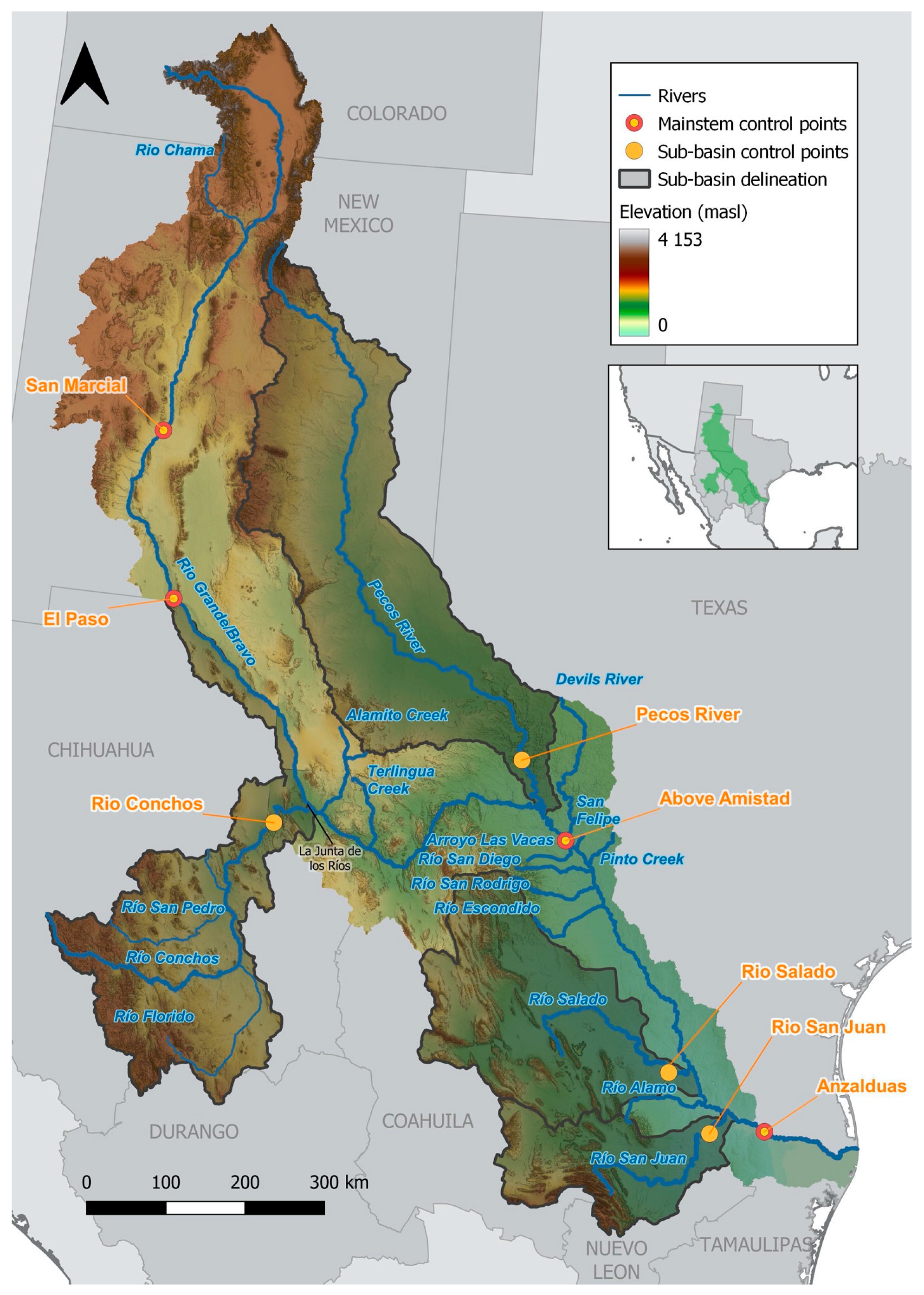
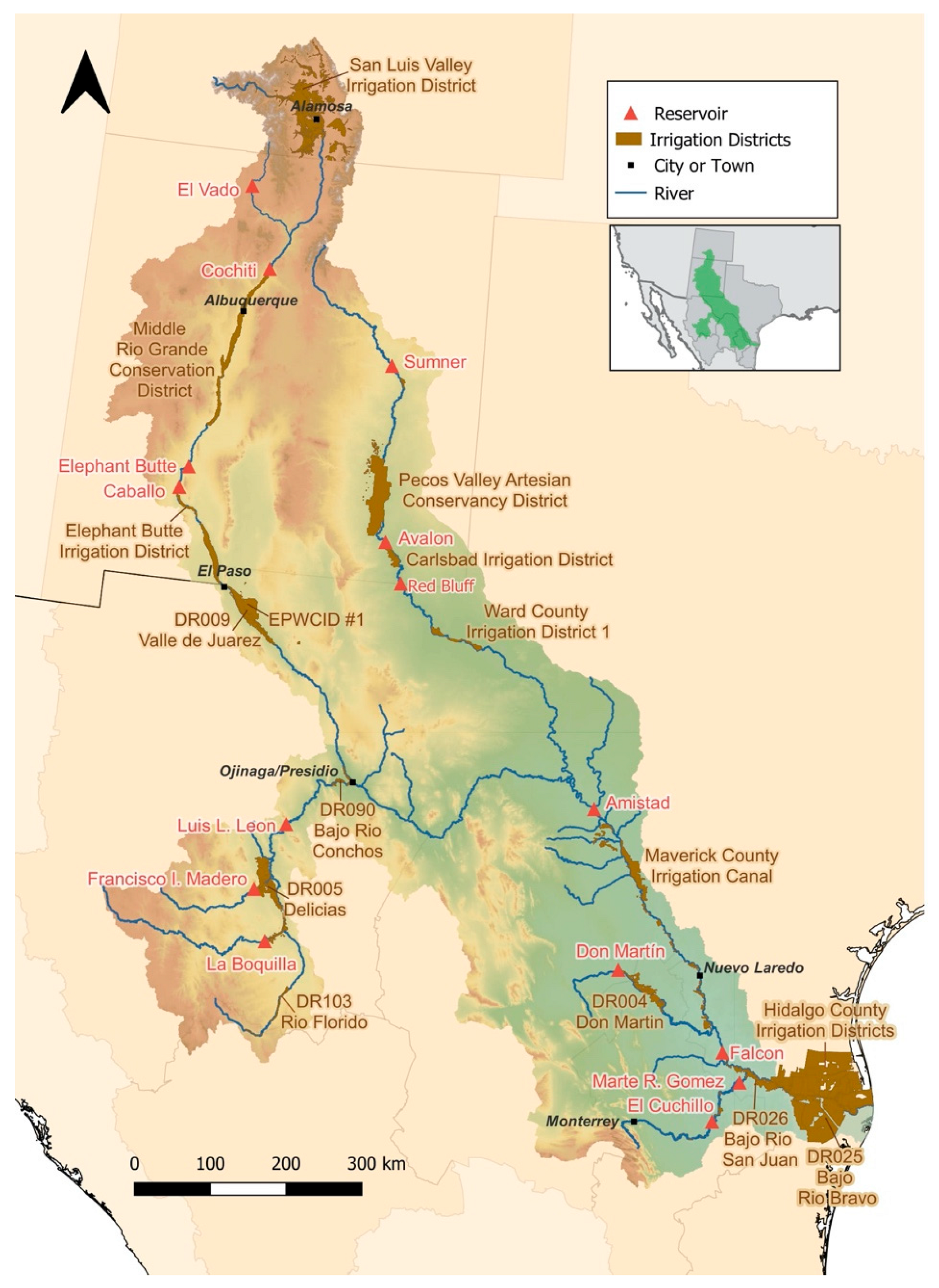
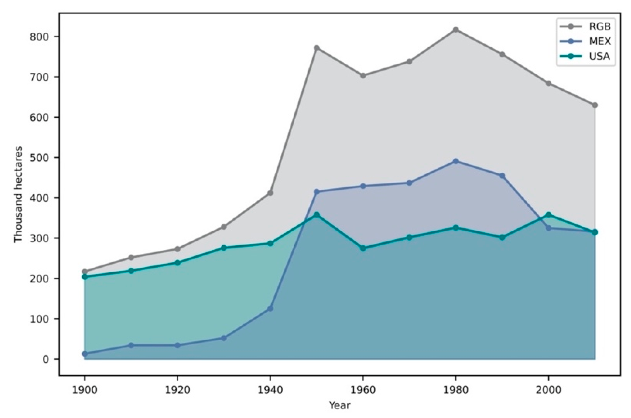
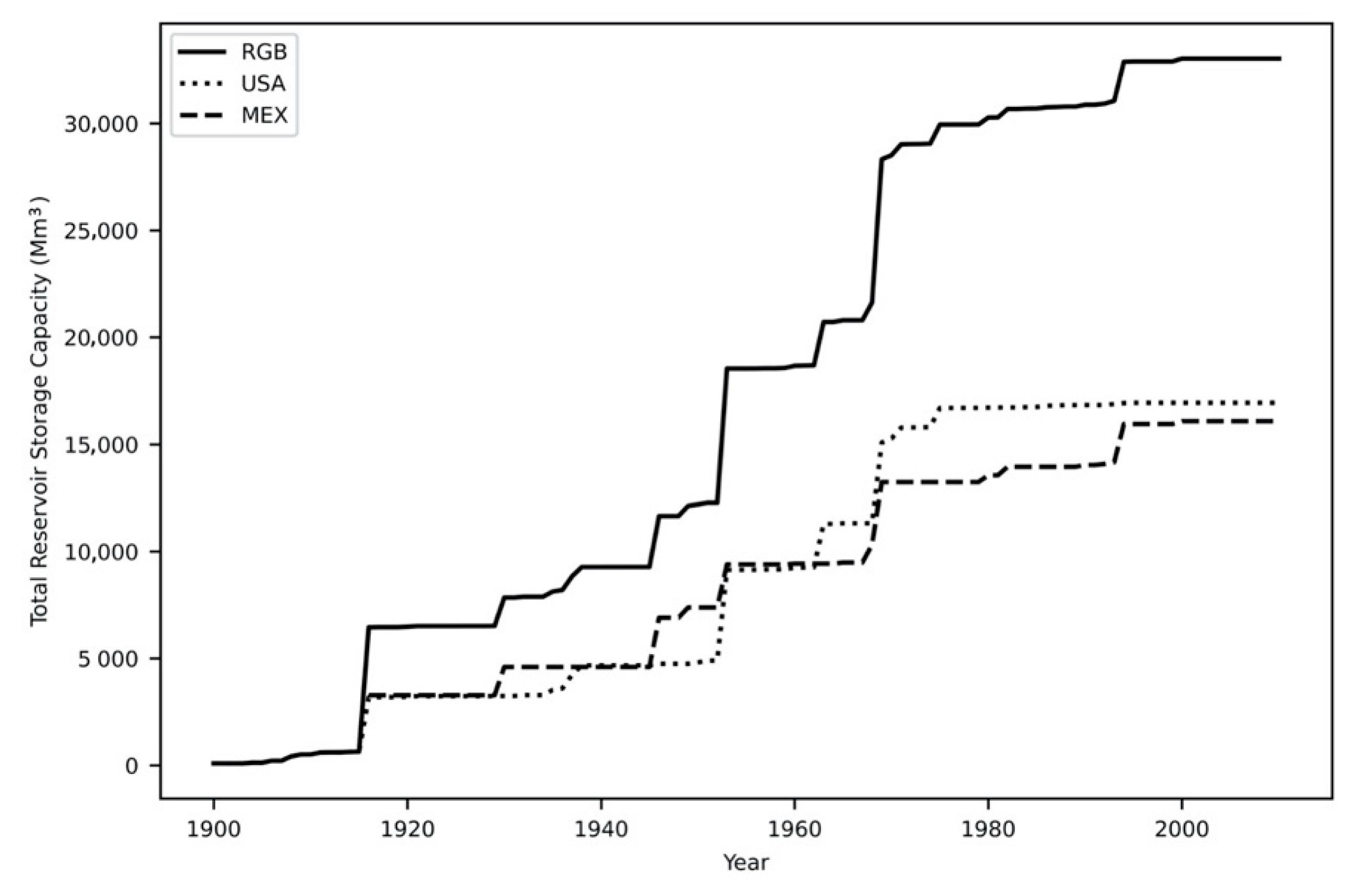
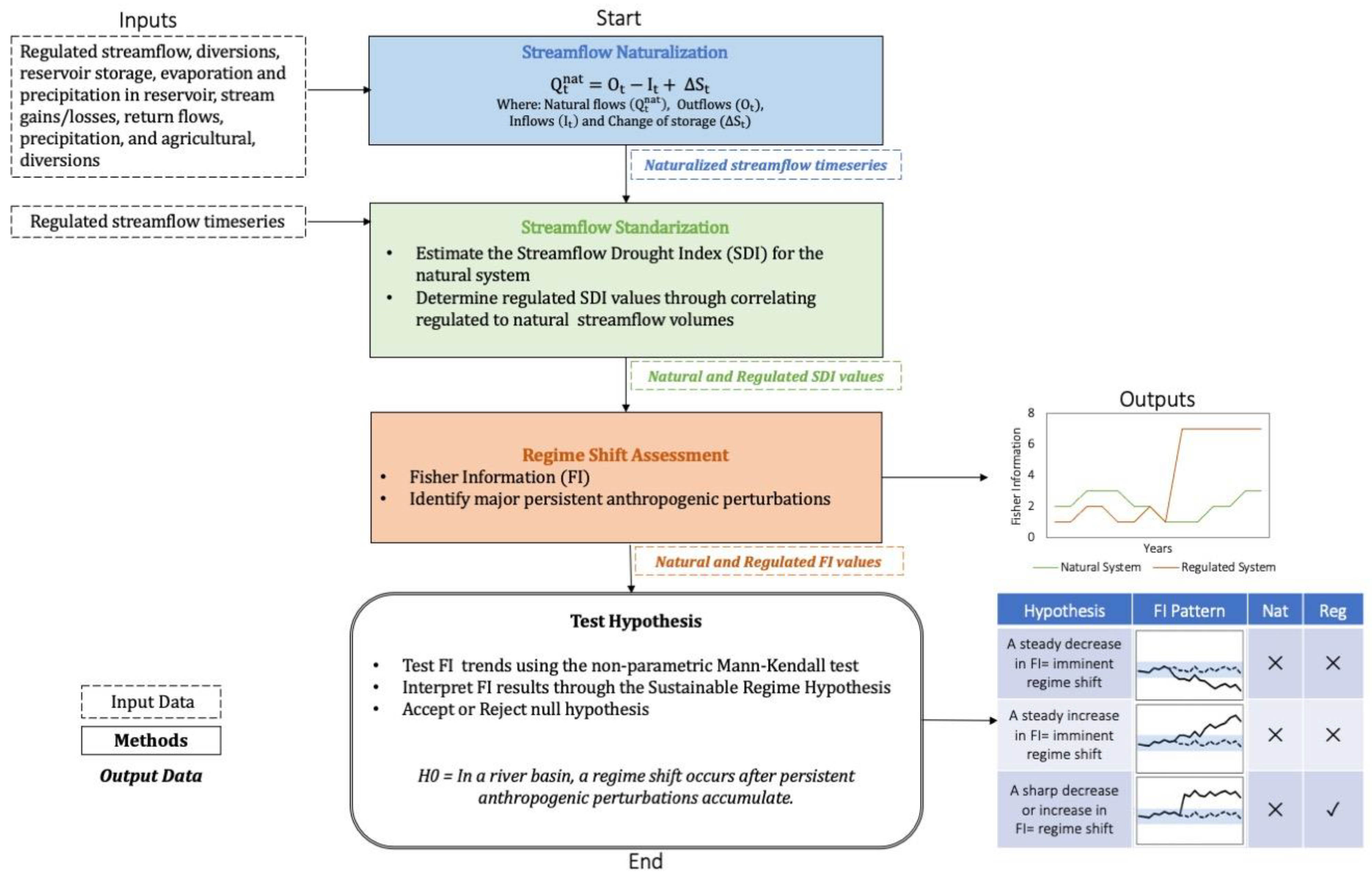
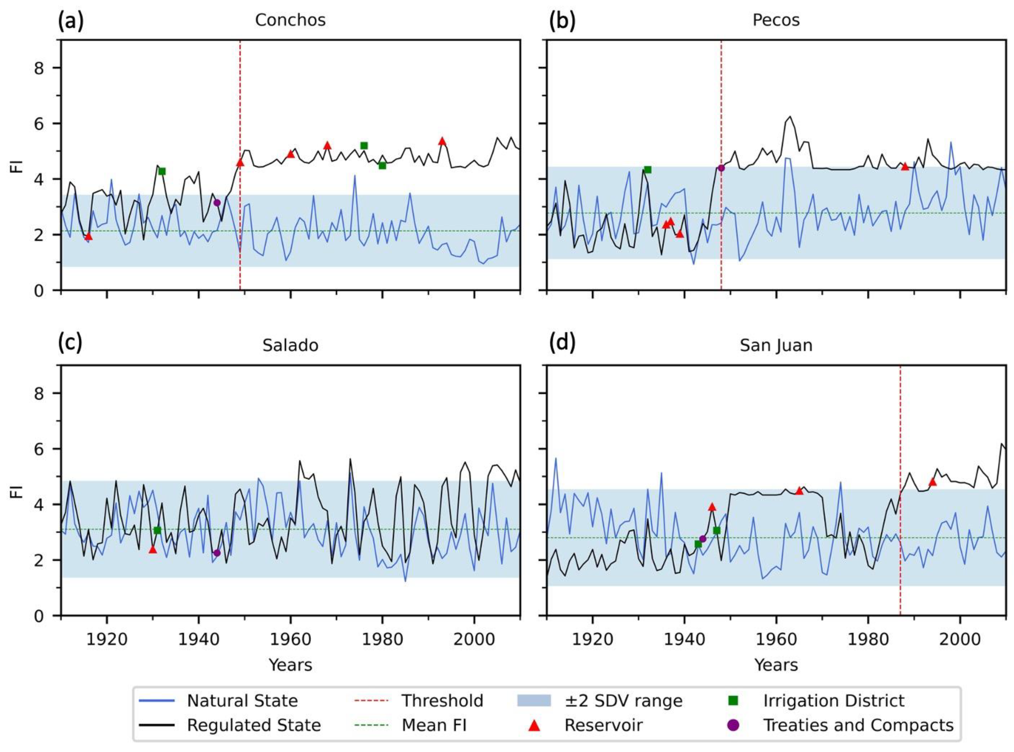
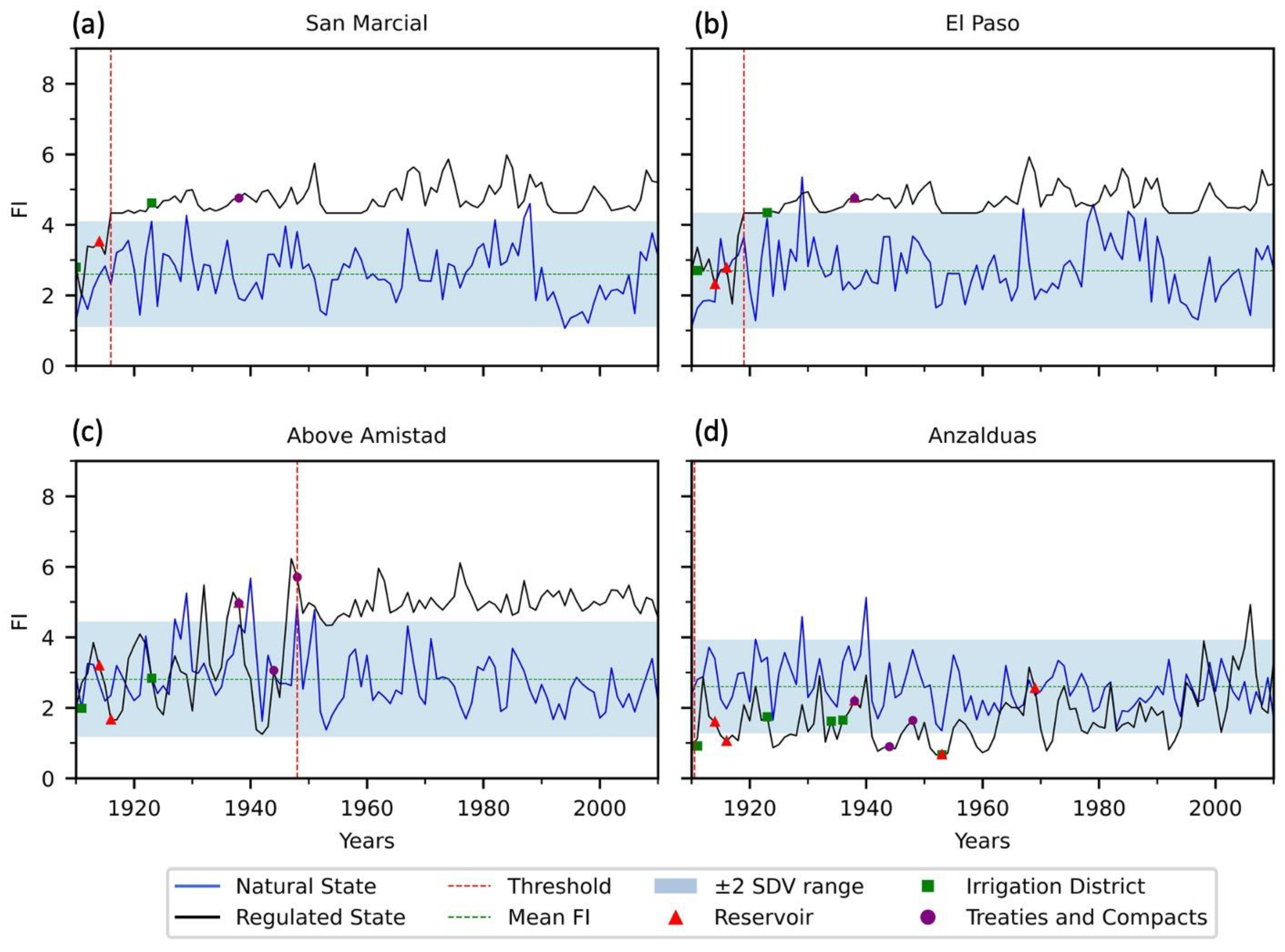
Table 1.
Statistical comparison of the estimated natural flows and the available studies of Orive de Alba [38], Loredo-Rasgado [37], and Blythe and Schmidt [33].
| Goodness of Fit Criteria | Orive-Alba | Loredo-Rasgado | Blythe and Schmidt |
|---|---|---|---|
| 1900–1943 | 1900–1944 | 1900–2010 | |
| Pearson’s Correlation | 0.990 | 0.995 | 0.996 |
| Coefficient of Determination (R2) | 0.995 | 0.998 | 0.998 |
| Index of Agreement (Willmott-d) | 0.995 | 0.995 | 0.995 |
| Coefficient of Efficiency (Nash-NSE) | 0.979 | 0.979 | 0.979 |
| Percent bias (PBIAS) | 3.589 | 7.131 | 1.881 |
Table 2.
Sustainable regime null hypothesis evaluation defined by the dynamics of the natural flow regime.
Table 2.
Sustainable regime null hypothesis evaluation defined by the dynamics of the natural flow regime.
| Sustainable Regime Null Hypothesis | Control Gauge Station | Naturalized Streamflow System | Regulated Streamflow System |
|---|---|---|---|
| A system is considered in an orderly dynamic regime when a nonzero FI remains nearly constant over time (i.e., d⟨FI⟩/dt ≈ 0). | Rio Conchos Pecos River Rio Salado Rio San Juan San Marcial El Paso Above Amistad Anzalduas | Accept | Accept |
| A steady decrease 1 in FI indicates that the system is losing its order, functionality, stability, and the patterns are breaking down. This declining trend may provide warning of an imminent regime shift. | Rio Conchos Pecos River Rio Salado Rio San Juan San Marcial El Paso Above Amistad Anzalduas | Accept Reject Accept Accept No trend No trend Accept Accept | Reject |
| A steady increase 1 in FI indicates that the system is becoming more stable and organized. | Rio Conchos Pecos River Rio Salado Rio San Juan San Marcial El Paso Above Amistad Anzalduas | Reject Accept Reject Reject No trend No trend Reject Reject | Accept |
| A sharp decrease or increase in FI indicates a regime shift | Rio Conchos Pecos River Rio Salado Rio San Juan San Marcial El Paso Above Amistad Anzalduas | Reject | Accept Accept Reject Accept Accept Accept Accept Reject |
1 The decrease or increase must be greater than two standard deviations from the mean FI for the entire time period [50]. Mann-Kendall decrease/Increase.
Publisher’s Note: MDPI stays neutral with regard to jurisdictional claims in published maps and institutional affiliations. |
© 2022 by the authors. Licensee MDPI, Basel, Switzerland. This article is an open access article distributed under the terms and conditions of the Creative Commons Attribution (CC BY) license (https://creativecommons.org/licenses/by/4.0/).
Share and Cite
MDPI and ACS Style
Garza-Díaz, L.E.; Sandoval-Solis, S. Identifying Thresholds, Regime Shifts, and Early Warning Signals Using Long-Term Streamflow Data in the Transboundary Rio Grande–Rio Bravo Basin. Water 2022, 14, 2555. https://doi.org/10.3390/w14162555
AMA Style
Garza-Díaz LE, Sandoval-Solis S. Identifying Thresholds, Regime Shifts, and Early Warning Signals Using Long-Term Streamflow Data in the Transboundary Rio Grande–Rio Bravo Basin. Water. 2022; 14(16):2555. https://doi.org/10.3390/w14162555
Chicago/Turabian StyleGarza-Díaz, Laura E., and Samuel Sandoval-Solis. 2022. "Identifying Thresholds, Regime Shifts, and Early Warning Signals Using Long-Term Streamflow Data in the Transboundary Rio Grande–Rio Bravo Basin" Water 14, no. 16: 2555. https://doi.org/10.3390/w14162555
Note that from the first issue of 2016, this journal uses article numbers instead of page numbers. See further details here.