Multivariate Statistical Analysis of the Phytoplankton Interactions with Physicochemical and Meteorological Parameters in Volcanic Crater Lakes from Azores

Abstract

This study aimed to identify the key factors influencing the phytoplankton development in four lakes on the island of São Miguel (Azores). We used a multivariate analysis of biological parameters (phytoplankton), physicochemical parameters, and meteorological data. Data were collected between 2003 and 2018 in the volcanic Lakes of Sete Cidades (Green and Blue), Fogo, and Furnas. The ecosystems of these bodies of water are increasingly vulnerable to anthropogenic activities (increasing human pressure) as well as to changing climate patterns. This analysis is the first exploratory approach to this dataset to explore trends and patterns of evolution from a multivariate perspective. This approach is also intended to improve understanding of the conditions that favor the emergence of different Cyanobacterial divisions. For this purpose, several statistical and chemometric methods were used, such as analysis of variance (ANOVA) and principal component analysis (PCA). Multivariate models combining biological and meteorological data focused from 2010 to 2012. The results from the PCA models showed that the abundance of Bacillariophyta, Dinophyta, and Cryptophyta phyla are correlated and appear to be influenced by high levels of precipitation, evaporation, and wind speed. On the other hand, the Cyanophyta, Chlorophyta, and Chrysophyta phyla appear to be more correlated with high values of air temperature, water temperature, and radiation. Also, the Euglenophyta phylum appears to be associated with low levels of precipitation, evaporation and wind speed, and high temperatures. Finally, we can conclude that these lakes have endured physicochemical parameters over the past 15 years, meaning that the measures adopted to monitor and protect the lakes are effective.

1. Introduction

General Framework

The Azores is a Portuguese archipelago of nine islands located in the North Atlantic, between 37° to 40° N latitude and 25° to 31° W longitude. São Miguel Island, the largest and most populated island of the archipelago, is about 2000 km from the mainland. The archipelago is one of the outermost regions of the European Union.

The volcanic genesis of these islands explains the origin of various lakes in the Azorean landscape [1]. Some of the craters of ancient volcanoes have been filled with rainwater [2,3] and have become lakes, which are, presently, an important touristic attraction and are a valuable supply of water for irrigation, consumption, and recreation. However, the increasing pressure through anthropogenic activity has produced changes in water quality and eutrophication in many of these lakes, demanding a constant monitorization of its trophic state [4,5,6,7] by the Azorean Authorities [7,8], especially since the early 2000s. Additionally, the application of the Water Framework Directive of the European Union by the member states also gave rise to the development of new tools to avoid the eutrophication of water bodies [9]. On the other hand, as agroindustry is one of the main pillars of the Azorean economy, eutrophication is worsened by the excessive use of fertilizers on grasslands [10]. This results in a high amount of nutrients (nitrogen and phosphorus) in the lakes, which then causes algae (including cyanobacterial) to bloom [11], a phenomenon of particular concern due to their potential toxicity and unpleasant appearance. Eutrophication can also be attributed to an increase in water stratification, an adaptation of phytoplankton, or new environmental conditions [6,7,10,12]. Phytoplankton is a key element of lake ecosystems, having a high sensitivity to small environmental changes. His biomass, composition, and abundance phyla are controlled by several factors, such as solar radiation, temperature, nutrient enrichment, organic matter, pH, etc. [13,14]. Therefore, phytoplankton is considered a biological indicator of the lake’s trophic state [13,15]. In Azorean lakes, phytoplankton is characterized by its most common phyla, namely Bacillariophyta, Chlorophyte, Cryptophyta, Chrysophyta, Cyanophyta (aka Cyanobacteria), Dinophyta, and Euglenopyta [8,16], whose spatiotemporal variations can be affected not only by the trophic state of water bodies, but also by other factors such as temperature, precipitation, radiation, wind intensity, among others.

In recent years, phytoplankton blooms have occurred often and, according to climate experts, the incidence of these extreme events can also be due to climate changes [17,18], which represents a very complex combination of stressors, from rising temperatures to elevated atmospheric CO₂. Indeed, the United Nations Climate Change Conference (COP26) highlighted that the world is on track to be around 4.8 degrees warmer by 2100. The greenhouse effect happens due to the gas emissions absorbing infrared radiation, which increases the temperature. This phenomenon is also observed in the Azores. The results of phase 5 of the Coupled Model Intercomparison Project (CMIP5) [19], composed of about 39 models of global circulation, show the Azores archipelago represented by a rectangular area between 35° N–40° N and 25° W–35° W (located at North Atlantic). Over the past 20 years, there has been a positive trend of 0.12 °C per decade. As for precipitation, there is a negative trend of −133 mm/decade. These results show that the climate is already changing in the Azores. Results for Representative Concentration Pathways (RCP) scenarios such as RCP2.6 (hopeful) and RCP8.5 (hopeless) point out that an average annual temperature increase in the Azores is between 1 °C and 4 °C up to 2100, respectively. The RCP8.5 scenario also shows a decrease in the average annual precipitation in the Azores by about 1.65 mm/day by the end of the century [19]. Recently, C. Andrade et al. [20] suggested that eutrophication processes increased CO₂ emissions from lakes due to increased decomposition of organic matter and biological activity. Thus, eutrophication is the result of a complex interaction of physicochemical and biological processes [21] that affect phytoplankton dynamics. However, it is still unclear how the cumulative impacts of meteorological factors combined with the remaining processes affect phytoplankton dynamics. Although meteorological data have already been included in similar investigations [22], this effect is increasingly relevant because the climate is changing. For example, in Lake Segara Anak, it was evidenced by Principal Component Analysis (PCA) that environmental factors and the increase in nutrients had an influence on the composition of phytoplankton [23]. Bashiri et al. [24], in a study to classify the trophic state of Dez Reservoir, used PCA models to understand the eutrophication of the water, which demonstrated the potential effect of eutrophication classification, and consequently showed its ability for pattern recognition of this phenomenon. A study performed by Stefanidis and Papastergiadou in nineteen Greek Lakes showed that PCA models are important to distinguish key morphological parameters [25]. Parineta et al. states that PCA models, made with correlation coefficients, are an appropriate tool to make precise descriptions of the water quality [26].

This work aims to identify multivariate correlation structures between biological (phytoplankton phyla), and physicochemical and meteorological datasets recorded over several years in four volcanic crater lakes located on São Miguel Island (Figure 1). To accurately extract results from so many datasets, including spatial and temporal records, we employed a multivariate analysis tool (PCA) which was successfully used to analyze a combination of multiple factors that influenced the phytoplankton abundance and water quality state [12,22,23]. We carried out a thorough evaluation of the original data, which has allowed us to identify unseen correlations between the parameters studied.

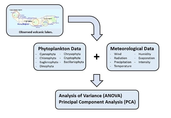
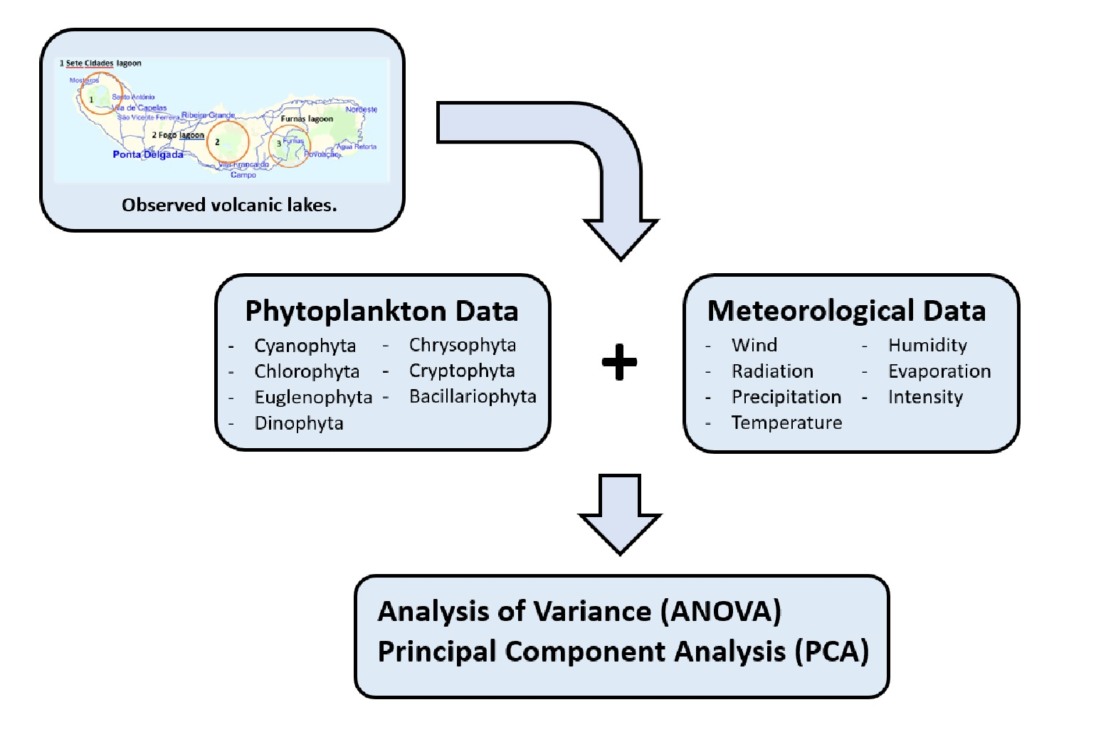
2. Materials and Methods

2.1. Study Lakes

S. Miguel Island (Figure 1) is in the oriental group of the archipelago, between 37°55′ N to 37°04′ N of latitude and 25°52′ W to 25°08′ W of longitude, it has a length of 66 km and a maximum width of 16 km, has an area of about 744 km² and 137,220 inhabitants (year 2020) [27]. Sete Cidades lake (A in Figure 1) is located at 260 m above sea level and is subdivided into two lakes, the Blue Lake (1 from A in Figure 1) and Green Lake (2 from A) in Figure 1), rising a total surface area equal to 4,46 km². Blue Lake has a maximum depth of 29 m, a surface area of 3.6 km², a volume of 47,361 m³, a length of 2590 m, and a width of 2093 m. The Green Lake is smaller, with a maximum depth of 26 m, an area of 0.9 km², 10,679 m³ of volume, 1540 m in length, and 777 m in width [9]. Both lakes have grasslands around, and a small village is located close the Blue Lake [2]. Fogo lake is located at an altitude of 575 m, with an area of 1.48 km², a maximum depth of 30 m, a volume of 18,040 m³, 2203 m of length, and 1010 m of width [9]. Due to its geographic localization, it is less affected by human activity, having vegetation and streams around it. Lastly, Furnas Lake is located at 280 m above sea level, 1.48 m² of the surface area [7], a max depth of 12 m, a volume of 9212.5 (m³), a length of 2045 m, and 1485 m of width [9]. Furnas Lake has grasslands around it and hydrothermal activity in the northern margin [28]. These lakes were chosen because they are the main and largest on the island.

Sete Cidades Lake has an average water temperature between 13.4 °C and 17.7 °C [6]. Thermal stratification is significant during the summer periods, especially in Sete Cidades and Fogo Lakes, in which different temperatures are observed in the epilimnion and hypolimnion [2,6,28]. According to Cruz et al. [6], Furnas Lake has a low O₂ content due to organic decomposition, but the lake has the highest concentration of CO₂ which implies that it is of volcanic origin [29] due to hydrothermal vents and fumaroles on the lake shores. Antunes [2] states that Furnas Lake does not stratify, but the lack of wind and rain during the summer allows the deeper regions of the lake to do so, decreasing the dissolved oxygen in the hypolimnion, while increasing the concentration of CO₂ [29].

The average values of the Trophic State Index in the period 2013–2016 classify Lake Furnas and Green Lake from Sete Cidades as eutrophic [8,30,31], while Fogo Lake and Blue Lake from Sete Cidades were classified between the states of oligotrophic and mesotrophic [8,30]. The Blue Lake from Sete Cidades and the Fogo Lake were both classified as oligotrophic, respectively in 2014 and 2015, getting the best water quality status [8,31].

Due to their location, the lakes differ in terms of the extent of vegetation cover, surrounding villages, and accessibility, presenting waters with distinct physicochemical and biological characteristics; also exhibit local specific atmospheric conditions.

2.2. Available Data

The data used for this study were available from the website http://www.azores.gov.pt/Gra/srrn-drotrh/menus/principal/Monitorização of the Regional Water Monitoring Authority [32] (accessed on 25 March 2020), which, since the early 2000s, has assessed the water status of lakes. The data available for analysis included datasets of phyla and phytoplankton (designated biological I), trophic status, cla and pheo (designated biological II), and physicochemical parameters, respectively corresponding to datasets A, B, C, and D, as well as meteorological (data set E) (

Table 1. A summary of data available for analysis (biological, physicochemical, and meteorological).

(Data Set)	Time Range	Number of Sampling Points	Number of Descriptors	Number of Lakes	Depths of Sampling	Seasons
A	2003–2018	837	8	4	5	4
B	2003–2018	853	5	4	N/A	4
C	2003–2018	1369	2	4	4	4
D	2003–2018	1482	30	4	3	4
E	2010–2012	979	8	4

Notes: Depths of sampling were 5 in total: surface, middle, button, composed, euphotic; Seasons: Spring, Summer, Fall, Winter; N/A–not applicable.

). All data were available in Excel sheets including the details about the sampling methodology and measurements. Data set A has been collected seasonally (once in each of the 4 seasons), while data sets B, C, and D were collected monthly, all covering the period 2003–2018. The meteorological data set (E) was collected daily (covering 24 h per day) from 2010 to 2012 by automated meteorological stations positioned near the study lakes. In this case, only daily maximum values were selected.

The sample dates covered all 4 seasons, which were defined as winter (January, February, March), spring (April, May, June), summer (July, August, September), and fall (October, November, December).

All datasets of the studied samples are described in

Table 2. The data groups and variables in each group.

Data Set	Scope	Descriptors (Variables)
A	Biological I (phytoplankton phyla)	Cyanophyta (aka. Cyanobacteria), Chlorophyta, Euglenophyta, Dinophyta, Chrysophyta, Cryptophyta, Bacillariophyta and unidentified flagellated organisms abundance (cell/L) and biomass (10−9 mg/L).
B	Trophic state	Total phosphorus (µg/L), chlorophyll a (µg/L), Secchi disk transparency (m), Total Nitrogen (mg N/L), and dissolved oxygen (OD) (% saturation).
C	Biological II (cla and Phaeo)	Chlorophyll a (µg/L) and phaeopigments (µg/L)
D	Physicochemical	Total Acidity (mg CaCO3/L), Total Alkalinity (mg CaCO3/L), Aluminum (µg Al/L), Ammonium (µg NH4/L), Inorganic Nitrogen (mg N/L), Kjeldahl Nitrogen (mg N/L), Organic Nitrogen (mg N/L), Total Nitrogen (mg N/L), Calcium (mg Ca/L), Chloride (mg Cl/L), Electrical Conductivity at 20.0 °C (µS/cm), Iron (mg Fe/L), Phosphate (µg P2O5/L), Inorganic Phosphorus (µg P/L), Organic Non-Particulate Phosphorus (µg P/L), Total Organic Phosphorus (µg P/L), Inorganic Particulate Phosphorus (µg P/L), Organic Particulate Phosphorus (µg P/L), Total Phosphorus (µg P/L), Manganese (µg Mn/L), Nitrate (mg NO3/L), Nitrite (µg NO2/L), OD (% saturation), pH (pH unit), Potassium (mg K/L), Sodium (mg Na/L), Sulphate (mg SO4/L), Temperature (°C), Secchi disk transparency (m), Turbidity (UNT)
E	Meteorological	Radiation (w/m2), Wind Speed (km/h), Precipitation (mm), Temperature (°C), Water Temperature (°C), Humidity (%), Evaporation (mm), Water Level (mm).

, which include dataset A (8 phytoplankton phyla descriptors), dataset B (5 trophic state descriptors), dataset C (2 biological parameter descriptors), dataset D (30 physicochemical parameter descriptors) and, finally, dataset E (8 meteorological parameter descriptors).

2.3. Statistical Analysis

The large number of datasets in this work requires Principal Component Analysis (PCA) to reduce its dimensionality and provide an easy processing, ranging from outlier detection to data visualization. This statistical method captures the maximum possible variation between datasets and displays the observations in uncorrelated vectors, called components. The use of this technique allows us to explain the total variability of the data with the smallest possible number of components [33]. A n-dimensional sample can be transformed by PCA into a lower d-dimensional one (d < n) while retaining as much of the variation present in the original dataset as possible. The process is performed by a linear transformation of the original set of characteristics into a smaller set of characteristics called principal components. These components are uncorrelated and hierarchically ordered. According to the Kaiser criterion [34], the first component (PC1) retains the greatest variance of the original data, the second component (PC2) explains the greatest variance not yet explained, and so on. The last component will be the one that makes the smallest contribution to explaining the total variance of the original data. In this study, only the first two main components were selected because each component showed eigenvalues > 1 [34,35]. When PC1 and PC2 are plotted against each other, it is possible to visualize the greatest variance in the data and find the relationships between the variables. The graph of scores evaluates data structure and detects clusters, outliers, and trends, while the graph of loadings serves to identify which variables have the greatest effect on each component. Both graphs are obtained by the PC1 × PC2 projection. Furthermore, the PCA also allows us to find underlying patterns between data. It is common to use a third graph, named biplot (which overlays the score graph and the loading graph), where the sample scores and variable loads are seen in a single graph. Before analyzing the data using PCA, outliers and missing data were identified and excluded.

2.4. Data Analysis

Data sets A, B, C, D were first analyzed separately following the plan exhibited in

Table 3. A multivariate analysis plan of each single dataset.

Data Set	Loading Plots (LP)	Score Plots (SP) Colored by	Biplots (n)
A	phytoplankton phyla: abundance and biomass (2)	(4) lakes, depths of sampling, seasons and years	(8)
B	trophic state (1)	(2) lakes and seasons	(2)
C	cla and phaeo (1)	(2) lakes and seasons	(2)
D	Physicochemical parameters (1)	(3) lakes, depths of sampling, and seasons	N/A
E	Meteorological parameters (1)	(2) lakes and years (3) years (observations in each one of the Lakes *)	(5)

Notes: * Furnas Lake, Fogo Lake, and Sete Cidades Lake (as just one: where data from Blue Lake and Green Lake has been joined); (n) is the number of biplots for each data set: n = $\left(LP\right)\sum \left(SP\right)$.

. Data set A (abundance) and data set E were then analyzed simultaneously, but only for the period between 2010 and 2012 following the plan shown in

Table 4. Multivariate analysis plan to join dataset A and dataset E.

Data Set	Loading Plots (LP)	Score Plots (SP) Colored by
A + E	abundance phytoplankton phyla + meteorological parameters (1)	(4) Lakes *, depths of sampling +, seasons, and years

Notes: * Furnas Lake, Fogo Lake, Blue Lake, and Green Lake; + surface and euphotic depths.

.

Data set A included in Table 4 corresponds only to the excerpt collected between January 2010 and December 2012. As mentioned above, this sampling was performed once a month (not specified) of each season (spring, summer, fall, or winter). Moreover, we selected only two sampling depth points, specifically one close to the surface (surface) and another close to the disphotic zone (euphotic). This methodology gives rise to a total of 96 samples (4 lakes × 4 sampling points × 2 depths × 3 years) in the considered time interval (the same as date set E). However, since the two temporal series do not match in data points (one is seasonal, and the other is daily) it was necessary to find days to match these two data sets before the application of multivariate analysis. Unfortunately, in the original data, it is not available neither the month nor day of phytoplankton collection (only the season). Due to this, it was assumed that phytoplankton samples were collected midway through each season, on the first day of every month (i.e., 1 November, 1 February, 1 May, and 1 August). In the case of the meteorology data, because of its sample inconsistency, frequency (for which we have a much more sampling frequency) was paired considering the median of the previous 15 days. So, for example, when pairing data for phytoplankton was obtained for 1 November, we consider the median of the meteorological data from the previous days (15 October to 1 November). After pairing, it was possible to validate a total of 47 samples. ANOVA tests were performed for all possible combinations of data sets A plus E, in all Lakes. Results were expressed in terms of the p-value. Those below 0.05 (95%) are normally considered statistically significant, although, in this study, the p-value of (0.1) 90% was the threshold considered for statistical significance.

2.5. Software

For data analysis, Microsoft Office Excel was used as a tool. After defining the parameters to be studied, the Matlab program, version R2016b (Mathworks, Natick, MA, USA) was used to perform ANOVA and PLS Toolbox version 8.2.1 for Matlab (Eigenvector Research, Manson, WA, USA) for the PCA models.

3. Results and Discussion

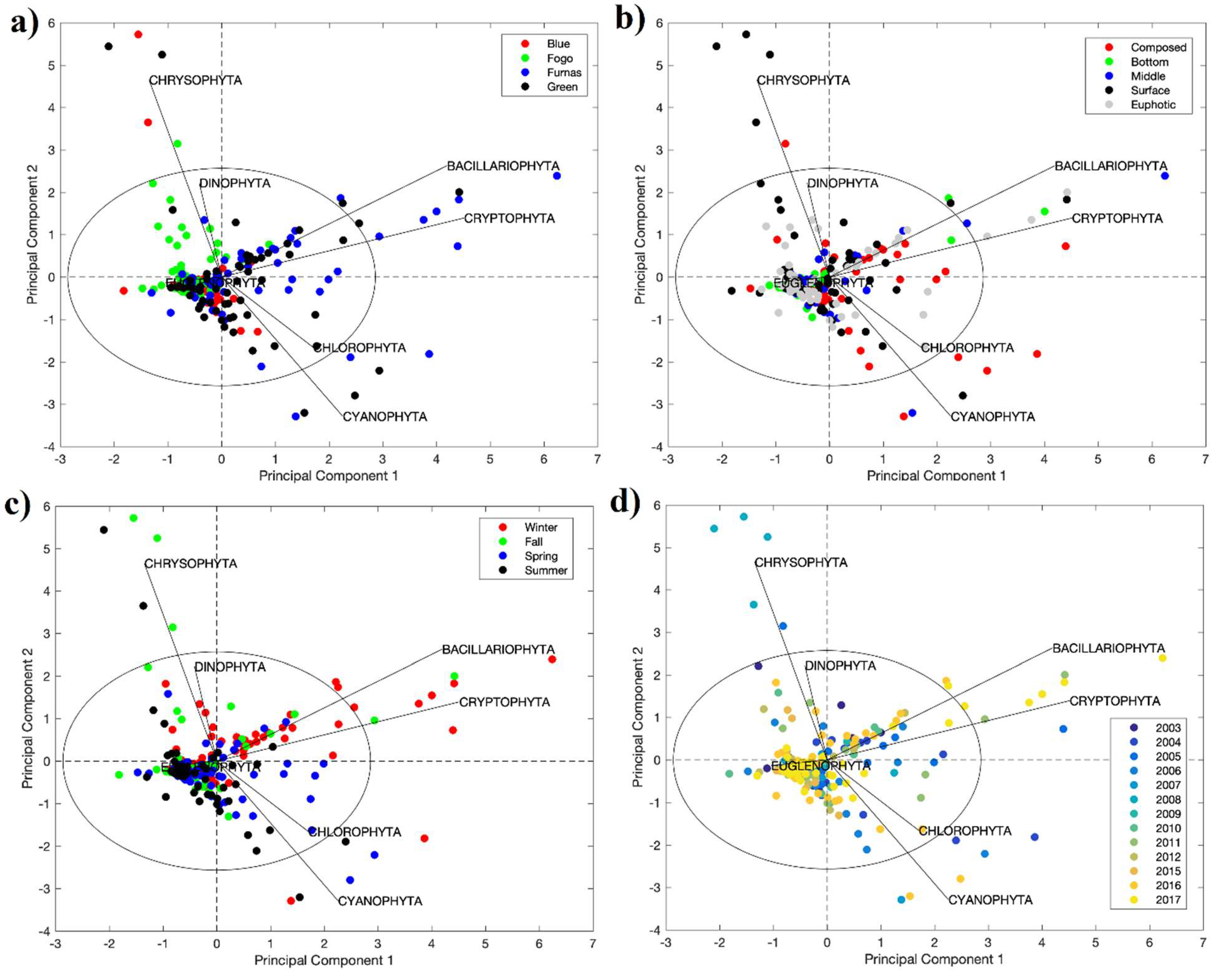
3.1. Multivariable Analysis for Phytoplankton

The analysis of the phytoplankton data set A was performed. The PCA decomposed data into the initial two principal components. Two models were constructed, respectively considering the abundance data (measured in cells/L), shown in the four biplots of Figure 2, and biomass data (measured in 10⁻⁹ mg/L), shown in the four biplots of Figure 3. The flagellated organisms were not considered for analysis as their values were 0 for all available samples.

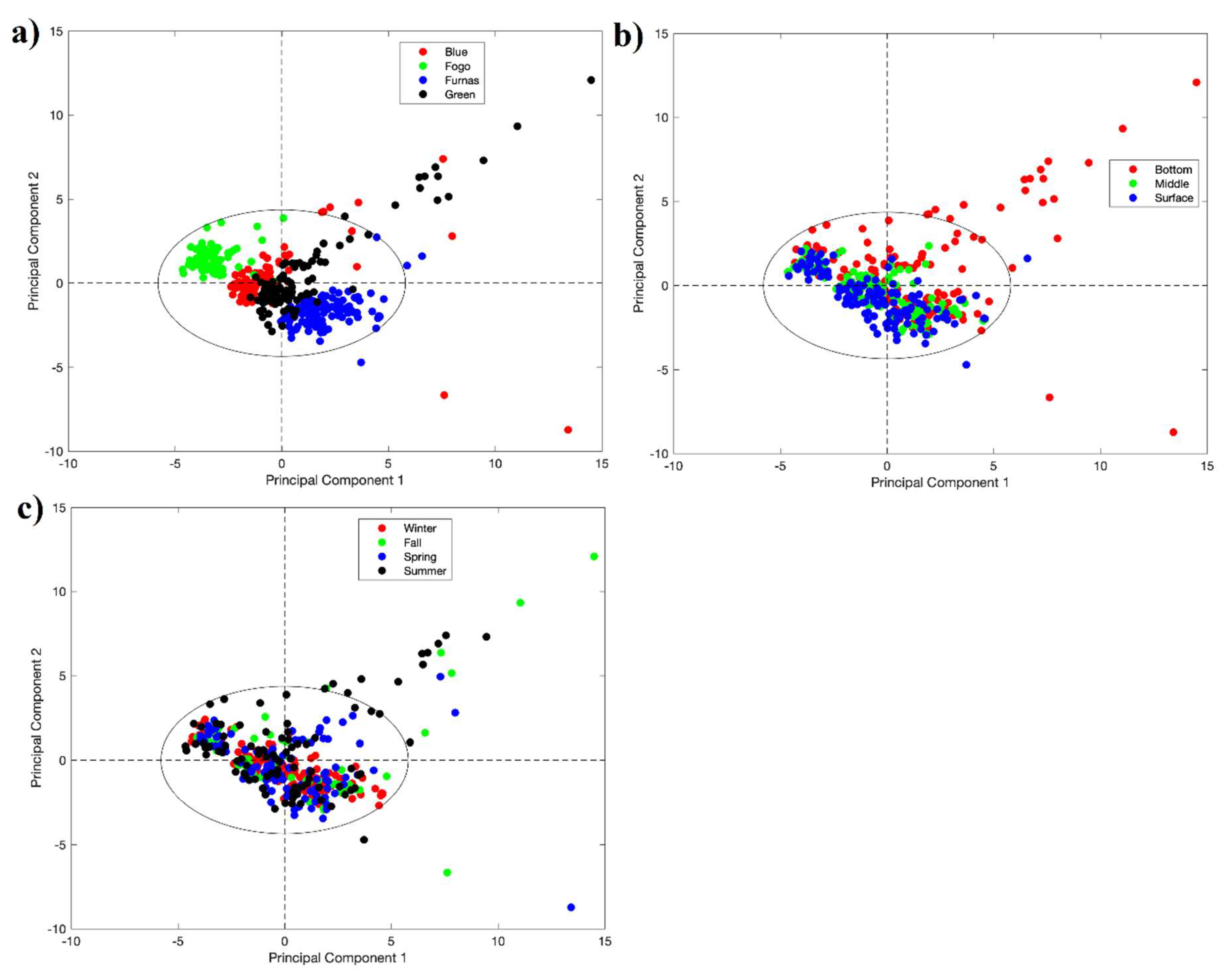
3.1.1. Phytoplankton Abundance

The PCA of the phytoplankton abundances shown in Figure 2 evidence correlations between the more abundant phytoplankton phyla found in the study lakes and identifies algal assemblages. For example, it appears that the Chlorophyta, Dinophyta, and Chrysophyta phyla always appear very close (2nd quadrant), meaning that there is a high correlation between these three phytoplankton phyla. On the right side, we can see that the Cyanophyta phylum is inversely correlated, while we can see that Cryptophyta and Bacillariophyta are not dependent on Chrysophyta or Cyanophyta phyla. This analysis criterion is the most used; that is, all variables whose angle between vectors is close to zero have a very positive correlation, angles of 180° have a very negative correlation and near 90° have little correlation. On the other hand, although most of the points are found to be located very close to the center without much variability, some are distant, corresponding to situations where the quantities of phytoplankton phyla increase far beyond the limit of the corresponding circle at the confidence interval. For example, in Figure 2a, the Bacillariophyta and Cryptophyta phyla (1st quadrant) appear in large quantities in Furnas Lake and Green Lake. However, this situation can be considered sporadic, having occurred only three times (three anomalous 4th quadrant points), which means that Cyanophyta appears very little in the Blue, Green, and Furnas Lakes.

By analyzing the graph of the scores for the first two major components for the sampling depth (Figure 2b), and once again analyzing the phytoplankton phyla in the 2nd quadrant, it is clear that the largest quantities correspond to samples taken on the surface or in the euphotic zone. Therefore, abundance typically has a higher correlation the closer to the surface the samples are taken. The remaining points, which correspond to a large majority, are in the central area of the graph and correspond to relatively low amounts of phytoplankton, for which it is indifferent to consider whether the sample was taken from lower (bottom) or middle levels.

For seasons (Figure 2c), the data indicate a certain distribution of phytoplankton phyla by distinct seasons. For example, Bacillariophyta and Cryptophyta (1st quadrant) appear essentially in winter, fall, and spring, but do not appear in summer.

In summer there is more of an association between Chlorophyta, Dinophyta, and Chrysophyta (2nd quadrant), but also in autumn. The data provider considers summer from July to September and autumn from October to December.

In terms of the period in years (Figure 2d), Bacillariophyta and Cryptophyta (1st quadrant) are more abundant in more recent years (2015–2017). On the other hand, Cyanophyta appeared in greater abundance in 2004–2005, but also in 2011. The chart also indicates that the Euglenophyta phylum, despite displaying low values over most years, appeared in great abundance in 2005 and 2009. In general, it is observed that the phyla Chlorophyta, Dinophyta, and Chrysophyta appear with some correlation with each other and with a negative correlation with Cyanophyta. On the one hand, Bacillariophyta and Cryptophyta are also positively correlated, but both are negatively correlated with Euglenophyta. The largest abundances of the Bacillariophyta and Cryptophyta association come from Furnas Lake and Green Lake. On the other hand, the largest quantities of the association Chlorophyta, Dinophyta, and Chrysophyta also appear in these two lakes, but also in Fogo Lake and, some traces, in Blue Lake. It is also noted that the highest abundance values of Bacillariophyta and Cryptophyta found in Green Lake and Furnas Lake came after 2015. Until 2010, Cyanophyta seems to have been quite isolated in the Sete Cidades and Furnas Lakes. Bacillariophyta and Cryptophyta tend to accumulate in all seasons except summer. According to Havens [11], cyanobacteria blooms are variable in some aquatic ecosystems, occurring persistent blooms throughout summer. A higher phytoplankton diversity was also found in summer, with enhanced cyanobacteria abundance [36]. There was a local dominance in some phyla [36], noticeably Chlorophyta, Cyanophyta, Dinophyta, and Euglenophyta between June and January.

3.1.2. Phytoplankton Biomass

For biomass data (Figure 3), the analysis is relatively similar to that of the abundance data, except that Chlorophyta appears to have a positive correlation with Cyanophyta (4th quadrant). These two phyla appear in Furnas Lake and Green Lake, which makes these two lakes very similar in terms of phytoplankton. This can be attributed to the leaching of nutrients from the pastures, through small streams and springs which bring more nutrients to be used by the algae. Warming temperatures of the lakes since there is also a correlation between the green algae and cyanobacteria with warmer seasons (summer) which leads to limited transport between layers causing lake stratification [28,29].

An anomalous occurrence of Chrysophyta is observed in 2006 (Figure 3d). The phyla Dinophyta and Chrysophyta appear essentially in the Fogo Lake and do not appear as often in the other lakes, although an extreme case occurred in the Green and Blue Lakes of the Sete Cidades (2nd quadrant). Also noteworthy is the case of Euglenophyta, which is barely visible until 2010, that is practically nonexistent before that year, but in recent years it has appeared in more quantities.

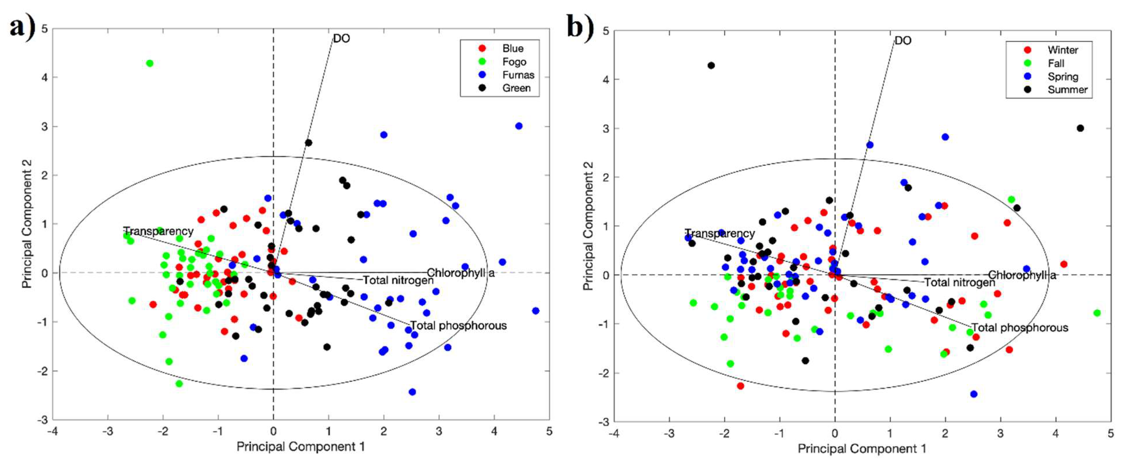
3.2. Multivariate Analysis of Trophic Data

The analysis of trophic data is highlighted in the ACP model scores shown in Figure 4. Results are displayed according to the bodies of water (lakes) and seasons. In terms of the correlations found, chlorophyll a and total phosphorus are found to have a relevant relationship to each other, but less to dissolved oxygen (DO). Once again, the Furnas and Green Lakes appear associated with the largest quantities [30,37]. In the case of chlorophyll, it is also verified that Green Lake has much more chlorophyll than Blue Lake. However, when looking at phytoplankton, it’s not evident the existence of a separation of populations between the two lakes. Regarding seasons, for example, it is observed that total phosphorus appears in greater quantities in summer and autumn (4th quadrant), which means that in these seasons some phenomenon must explain this behavior, perhaps due to warming of the water or increase of discharges into the lake, in particular the Furnas Lake, which is in fact where the most total phosphorus accumulates. In winter and spring, the scores are further back and closer to the center of the graph, which may be related to the thermal stratification of the lake as Furnas since in the summer and winter dissolved oxygen levels often stratify [30].

These results show a relative similarity between Furnas Lake and Green Lake, as already observed in previous models. In these lakes, but especially in Furnas Lake, chlorophyll a, total nitrogen, and total phosphorus are high, the last two might be from the fertilizers, leaching from the surrounding pastures close to the lake [9]. Lake Fogo has higher transparency and lower dissolved oxygen than the other three lakes. This means that it’s the lake that has less organic matter pollution and lower anthropogenic activity within its hydrographic basin [7]. The set of these five descriptors in this data set is indeed correlated and is therefore used to assess trophic status. Analysis of the results in terms of the season is, however, inconclusive. However, there is a tendency for higher dissolved oxygen levels in winter and spring, which might be because of the mixing of layers of the lake [29], and higher phosphorus content in summer and autumn. The lowest levels of chlorophyll are found in Fogo Lake.

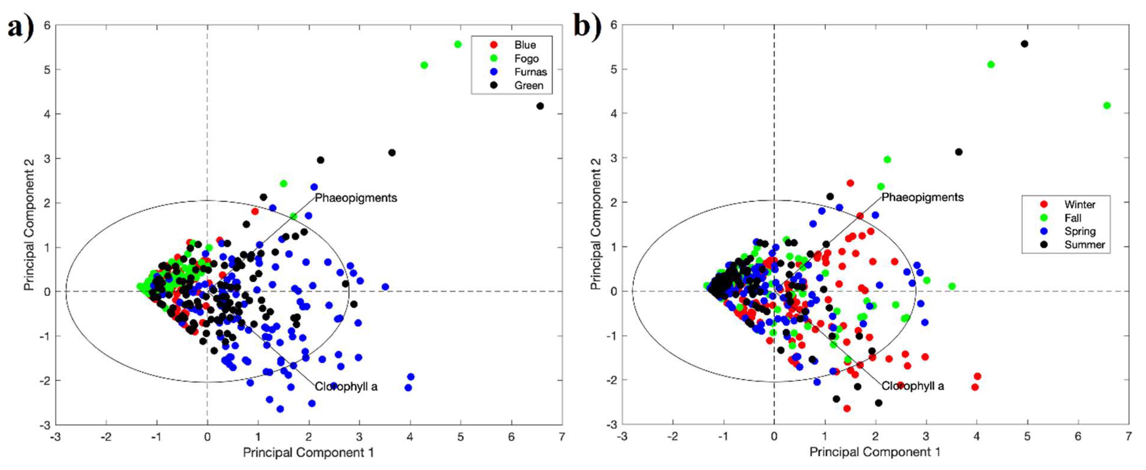
3.3. Multivariate Analysis of Chlorophyll a and Phaeopigments

Regarding the analysis of chlorophyll, a, and phaeopigments, the results are recorded in the scores in Figure 5. As phaeopigments may originate from chlorophyll a, some correlation between these two descriptors was expected. The respective correlation vectors establish an angle of about 90° to each other. For chlorophyll a, the data show similarities with those found in data set B. There are still phaeopigments in the Blue Lake, although in small quantities. However, it is essential in the Furnas and Green Lakes where they are in the greatest quantity. There are also traces in Fogo Lake. The score for the seasons of the year indicates that it is in autumn and winter that the phaeopigments are in greater quantities. These higher quantities of phaeopigments might be explained by the high hydrodynamics of these seasons [38].

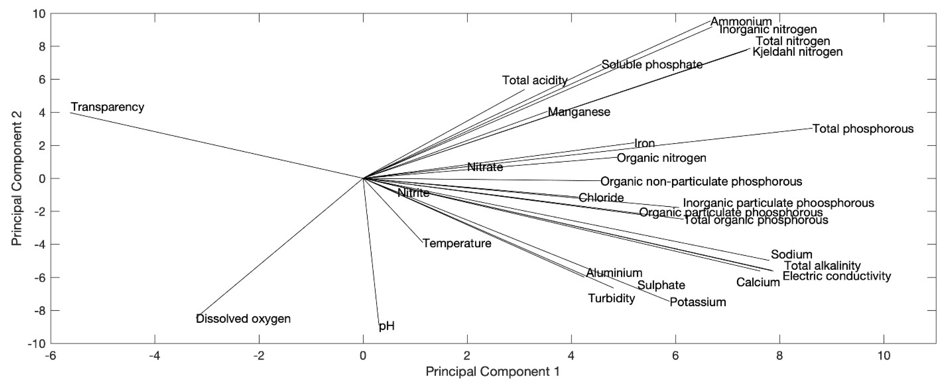
3.4. Multivariate Analysis of Physicochemical Data

Multivariate Analysis of physicochemical data is presented in Figure 6 for all lakes and can be interpreted as an average of what goes on in each one.

A first assessment of the correlation structure of these descriptors shows a clear opposition between transparency and the remaining descriptors. On the other hand, it can also be observed that nitrites and nitrates have a small variability, which is a good indication of the water quality index.

Some of the established correlations were already expected, namely the case of phosphorus, whose vectors are almost overlapping. However, there is a slight departure from the total phosphorus, which appears to have some relationship with iron and organic nitrogen. Nitrogen and ammonium (or ammoniacal nitrogen) are also virtually overlapping, which is expected due to their autocorrelation which means that both are coming from the fertilizers [11] used in the pastures around some of the lakes, as also from the sediment layer in the bottom of the lake that can be a source of phosphorus in the water [30]. It is observed that the temperature is little related to the other descriptors. In addition, there is some correlation between pH and dissolved oxygen, which in turn is negatively correlated with ammonium, but also with different types of nitrogen and total acidity. Turbidity is inversely correlated with transparency. Sulfates, aluminum, and potassium are positioned near turbidity. Sodium, calcium, alkalinity, and conductivity are positively correlated. The scores of the physicochemical data are shown in Figure 7. Figure 7a represents the analysis by water mass (by lake). The results very clearly show the different separate lakes, which means that they have distinct physicochemical characteristics.

Fogo Lake is separated from the others, Green and Blue are relatively overlapping, but not entirely, and Furnas Lake is opposed to Fogo’s. It was found that Blue Lake and Green Lake share some characteristics of the descriptors, although there are also some differences, that might be because of the state of eutrophication of the lake [8,29,30,31]. Some points, essentially in the Green Lake (1st quadrant) are outside the 95% confidence limit. When considering the information in Figure 6 (descriptor graph), these points are most likely displaced because of some variables, such as nitrogen, large amounts of nitrogen, which is not a very good sign, as it may mean the presence of fertilizers. On the other hand, in the 4th quadrant there are also points outside normal limits, but in this case in the Blue Lake, which may have to do with electrical conductivity or turbidity higher than normal. Electrical conductivity is a parameter that may indicate interference of anthropogenic actions on water quality of the lakes but also from their volcanic origins due to the hydrothermal fluids and fumaroles, which can be seen within Furnas caldera [6]. Those classified as oligotrophic have low electrical conductivity. On the other hand, eutrophic, or hypereutrophic lentic environments, which have low transparency, may be affected by anthropogenic activities and in which undesirable changes in water quality often occur [15].

Fogo and Furnas’s Lakes are two very distinct bodies of water in terms of physical and chemical descriptors. The greater transparency of the waters in Fogo’s Lake is obvious when compared to Furnas Lake, which is expected since the pastures along the Furnas Lake have their nutrients leached into the lake which in turn promotes the rapid growth of algae that in turn causes the turbidity [5,6,11]. It is found that Green Lake and Blue Lake are more susceptible to increased nitrogen levels during warm seasons (especially in summer and fall). These higher levels were detected when samples were collected from lower (background) levels. The Fogo Lake is diverted to the 2nd quadrant because it is substantially more transparent than the others.

In general, data indicate that the lakes are in good condition. Apart from some extreme points, which happen sometimes, there does not seem to be a great alarm situation, except for the presence of chlorophyll-a in the Green Lake. From this exploratory approach, it is possible to state that, despite some peaks observed in some lakes (mainly in the Sete Cidades Lakes) these lakes are quite resistant to changes, both in terms of phytoplankton and physicochemical parameters. Although we must consider lake stratification, anthropogenic activities, and volcanic secondary activities that can influence the presence of green and blue algae blooms. Also, anthropogenic activities could influence phytoplankton blooms. A similar study performed by Silva et al. [39] in a subtropical reservoir system showed a trend toward eutrophication due to decreased water transparency.

Over the last 15 years and even during the different seasons of the year [32]. Regarding the percentage of variance explained by the two main components, phytoplankton obtained 34.8% for abundance and, 35.2% for biomass; physicochemical got 40.6%, while the results for trophic state and chlorophyll a + phaeopigment were 85.5% and 100, respectively.

3.5. Multivariate Analysis of Meteorological Data

3.5.1. Multivariate Analysis of Meteorological Data Considering All Lakes

Figure 8 corresponds to the analysis of the climate data. Regarding the correlation between the variables, we have, for example, that the parameters radiation, water temperature, and temperature are positively correlated. But the same parameters are inversely correlated with the water level. Evaporation is positively correlated with precipitation and humidity, but less with wind speed. Figure 8a allows us to conclude that Fogo Lake is distinguished from the others by the high wind speeds it exhibits. On the other hand, it is also found that the weather data for Furnas and Sete Cidades lakes completely overlapping. In Fogo’s Lake, there is a mismatch relative to the position of the other, which means that from the climate point of view, Fogo Lake is different from the other two lakes. This difference might be the consequence of being at a higher altitude than the other lakes in the study [1,2], which also makes this lake less impacted by human activity [7].

Fogo Lake exhibits a different climate and displays more extreme values of these meteorological variables. In Figure 9b we have the coloring per year. The results show no major differences, although in 2011 there are some extreme points, as well as in 2012. Apparently, between 2011 and 2012 it began to change, because in 2010 the points are much lower and much closer to the center, i.e., the region of small variability. In 2012 changes begin to occur, all related to more extreme values of humidity, evaporation, and precipitation.

3.5.2. Multivariate Analysis of the Meteorological Data Segregated by Lake Variety

Figure 9 corresponds to the analysis of the weather data for each one of the lakes. Figure 9a refers to Furnas Lake, where there are some extreme precipitation points in 2012, but otherwise, there are no appreciable changes. These extreme points of precipitation do not mean, however, evidence of some climate change, they are only occasional situations that happened in those 5 days (the 5 points referred to correspond to 5 days of the 3 years of the sampling period). The correlation between variables is similar when comparing the three lakes, although with some minor differences, namely the case of radiation, which in this case appears inversely correlated with the wind speed.

In Sete Cidades Lake (Figure 9b), were occurred in 2012 more extreme points, essentially humidity, evaporation, and precipitation. In Fogo’s Lake (Figure 9c), there is a similar situation, but not the same as the previous ones, due to the appearance of more extreme points in 2011, and less in 2012. Regarding the correlation of variables, it is found that the water level is more correlated with the variables found in the 2nd quadrant (e.g., wind speed), which was not the case in the remaining lakes. Elçi [40] stated that lagged wind speed is one of the most influential parameters for water quality, which might happen because of the water level [41] Concerning the percentage of variance explained by the two main components, Furnas, Sete Cidades, and Fogo Lake got 54.1%, 53.7% and, 49.0%, respectively. All lakes obtained 50.1%.

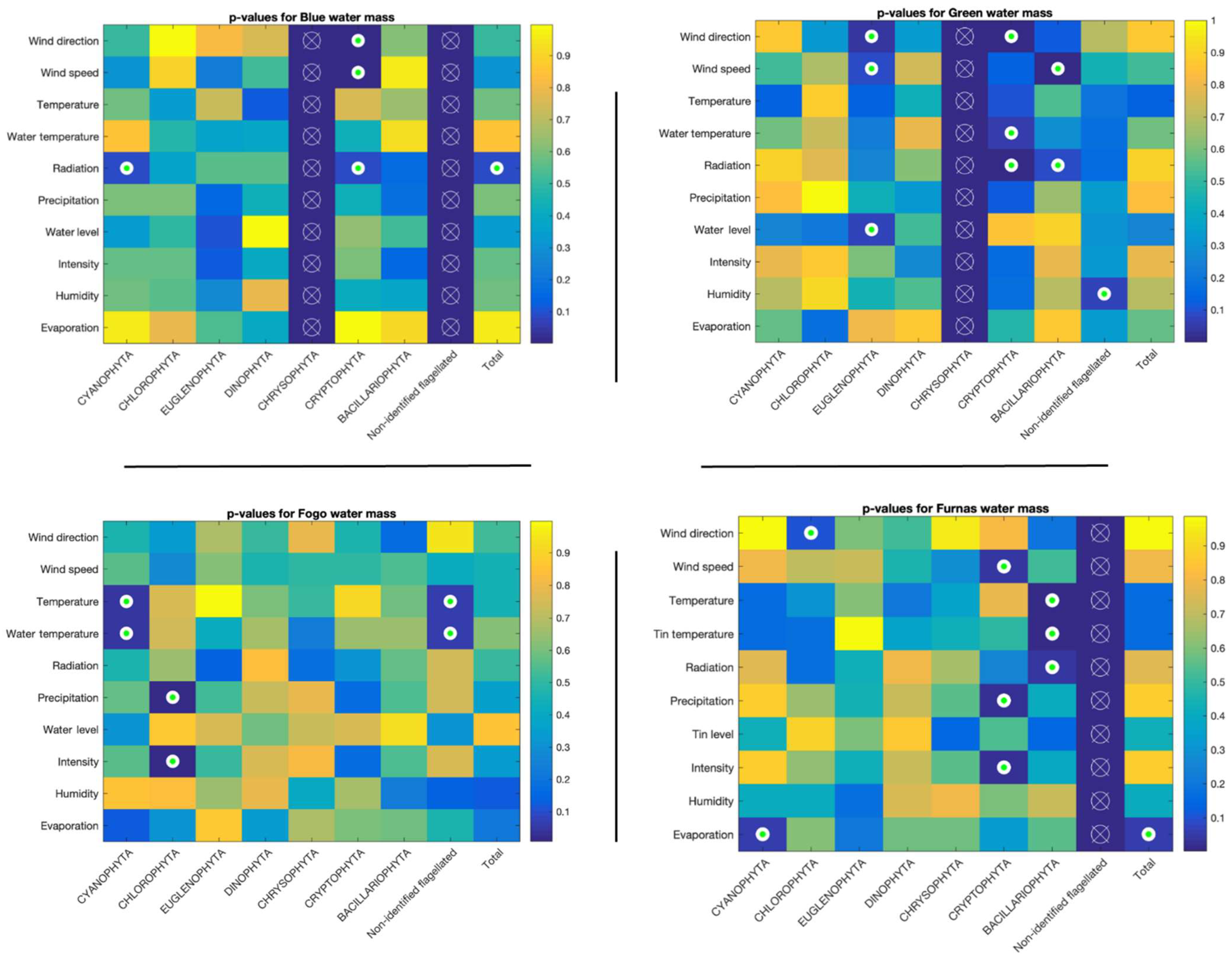
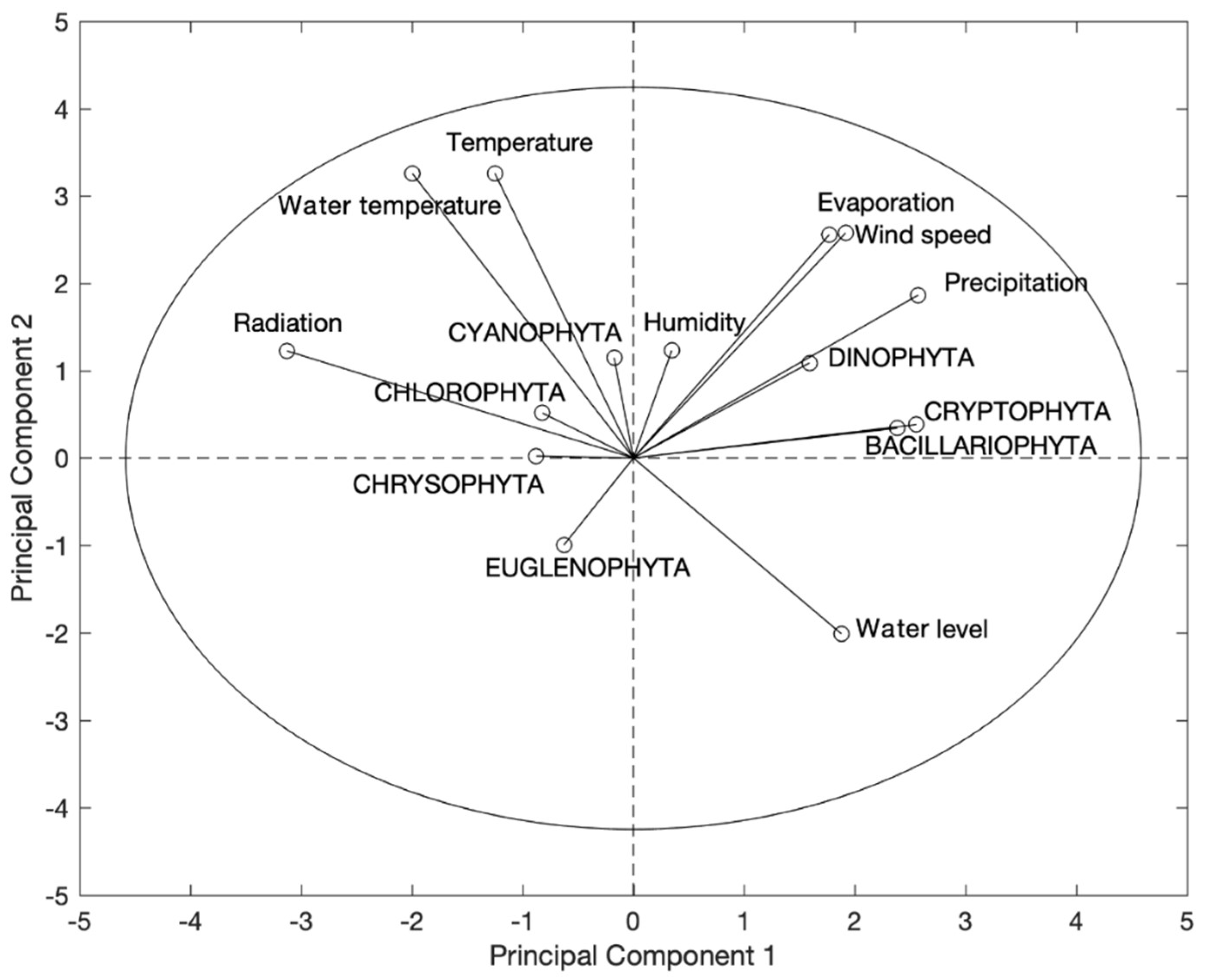
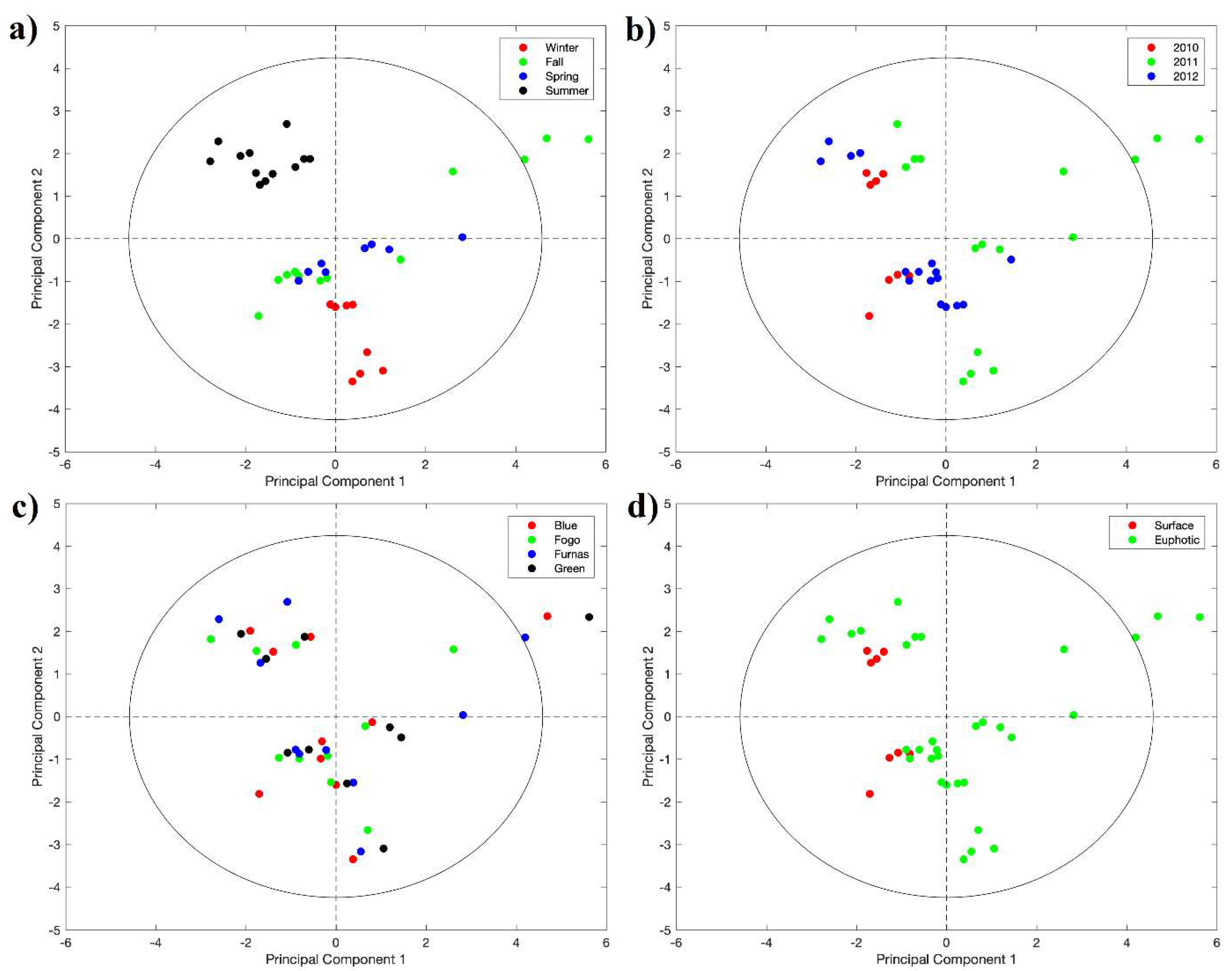
3.6. Multivariate Analysis of Phytoplankton and Meteorological Data

Afterward, PCA analyses were performed for the data set A and data set E individually, to understand how the abundance of different phytoplankton phyla correlates with the meteorological variables, and which meteorological variables may explain the variability observed in the various phytoplankton phyla. For this purpose, the data set A (abundance) and data set E collected in the Sete Cidades lakes (Blue and Green), Fogo and Furnas were analyzed simultaneously and restricted to the period between 2010 and 2012. A variance test using ANOVA was also performed.

Variance Analysis

Figure 10 shows the values of each of the seven phytoplankton phyla, including non-flagellate and totals, respectively to Blue Lake, Green Lake, Fogo Lake, and Furnas Lake. For ANOVA only two classes were considered for each phytoplankton phylum. The threshold that defines the separation of phytoplankton values in two classes to perform the ANOVA test is represented by the horizontal line (in red) and was estimated considering the observed distribution.

The analysis of the distribution of the values of each division of the phytoplankton allowed us to define the threshold levels necessary to divide the data into two classes: low values and high values. The results found for each limit are shown in

Table 5. Threshold levels considered for each phytoplankton phylum in every lake.

Lakes	Cyanophyta	Chlorophyta	Euglenophyta	Dinophyta	Chrysophyta	Cryptophyta	Bacillariophyta	Unidentified Flagellates	Total
Blue	1.26 $\times {10}^7$	6.75 $\times {10}^3$	9.74 $\times {10}^3$	3.00 $\times {10}^4$	2.69 $\times {10}^{-1}$	3.56 $\times {10}^5$	9.12 $\times {10}^5$	2.45 $\times {10}^{-1}$	2.00$\times {10}^7$
Green	9.37$\times {10}^7$	6.84 $\times {10}^6$	6.20 $\times {10}^3$	2.60 $\times {10}^4$	2.39 $\times {10}^{-1}$	3.72 $\times {10}^5$	1.14 $\times {10}^7$	1.84 $\times {10}^3$	1.01 $\times {10}^8$
Fogo	3.01 $\times {10}^6$	6.58 $\times {10}^6$	9.43 $\times {10}^3$	1.81 $\times {10}^4$	7.03 $\times {10}^4$	5.37 $\times {10}^4$	8.56 $\times {10}^6$	1.99 $\times {10}^3$	1.51 $\times {10}^7$
Furnas	9.02 $\times {10}^8$	2.74 $\times {10}^7$	2.72 $\times {10}^3$	3.57 $\times {10}^3$	9.38 $\times {10}^3$	8.61 $\times {10}^5$	4.47 $\times {10}^6$	1.34 $\times {10}^{-1}$	1.36 $\times {10}^9$

.

Figure 11 graphically shows the p-values obtained from every single lake. For some combinations, p-values could not be obtained because data were missing or because the variation was null (signaled by the marker ⊗). The p-values were colored according to a scale between 0 and 1. Values below the limit value of 0.1 were identified with a circle filled with a green dot.

The results obtained from the p-values do not show many statistically significant relationships. However, we consider the existence of a relatively considerable fraction of tests that produce statistically significant results but without remaining consistent in the different water bodies. This occurs perhaps because the test was performed considering each lake separately and the number of samples used for each test was reduced. Therefore, a new (multivariate) analysis was performed considering all volcanic lakes simultaneously, using a resampling method, to assess the confidence interval of the estimations for scores and loadings. Figure 12 exhibits the PCA analysis performed on the combined data set A and data set E and shows how the considered descriptors are correlated, considering all lakes simultaneously. The principal components represented (1st and 2nd) capture approximately 44% of the total data variation. For example, the abundance of Bacillariophyta, Dinophyta, and Cryptophyta are correlated and appear to be influenced by high levels of precipitation, evaporation, and wind speed.

On the other hand, Cyanophyta, Chlorophyta, and Chrysophyta seem to be more correlated with high values of air temperature, water temperature, and radiation. Pitois et al. [42] said that Cyanobacteria are associated with climatic domains related to temperature, global radiation, and pluviometry which goes our work supports regarding temperature and radiation variables. Euglenophyta seems to be associated with low levels of precipitation, evaporation and wind speed, and high temperatures. The analysis of the combined data, without the descriptors, is highlighted in Figure 13, considering different color schemes (by season, year of collection, water mass, and sampling depth). The analysis of Figure 13 should be done in combination with Figure 12, which serves as an indication for specimen differentiation. In Figure 13a, it is possible to see essentially two regions of clusters and some northeast-oriented samples (1st quadrant). One possible way of interpreting this graph is to explain the clusters. For example, in the case of Figure 13a, colored by season, it is very evident that the samples are grouped according to the season, with two clusters quite well defined for summer and winter. In summer there is a positive correlation between air and water temperature, as well as radiation, and in winter there is a negative correlation with these parameters. It is also possible to verify that the samples directed to the northeast were all observed in the fall, showing extreme precipitation values, corresponding to rainy days in this season. By analyzing the color chart by year of the collection (Figure 13b), the northeast samples all relate to the year 2011. According to the September 2011 IPMA Bulletin [43], extreme phenomena have been reported at the level of precipitation intensification in S. Miguel due to an anticyclone located southeast of the Azores in conjunction with hot and humid air mass. Even according to the IPMA bulletin there was a tornado in São Miguel on 26 November 2011 [43]. Therefore, the information taken from the graph in Figure 13b follows the meteorological information, also with Figure 12, where it is possible to explain this extreme variation (precipitation, wind speed, and evaporation). Figure 13c indicates that the samples do not exhibit affinity for lakes, not clustering on this score, and it is finally apparent from Figure 13d that most samples were collected in the euphotic zone.

4. Conclusions

This study aimed to highlight the relationships between information collected from four volcanic lakes on the island of S. Miguel (Azores), including biological, physicochemical, and meteorological information. The study aims to highlight relationships by promoting a multivariate analysis without focusing on explaining in detail the relationships identified. For this purpose, several multivariate models were elaborated upon based on the principal component analysis. The multivariate analysis allowed a better interpretation of the set of water quality monitoring parameters of the Azores lakes collected from 2003 to 2018, and meteorological data, although in this case only in the years 2010 to 2012. Despite the trophic state, of the phytoplankton community density and composition, the amount of chlorophyll a, etc., originated from the complex conjugation of several factors, it was possible to achieve the proposed objective, and to show some relevant relationships, highlighting the following:

• The highest abundance values for Bacillariophyta and Cryptophyta found in Green Lake and Furnas Lake came after 2015.
• By 2010, Cyanophyta appears to have been quite isolated in the Sete Cidades and Furnas Lakes.
• Bacillariophyta and Cryptophyta tend to accumulate in all seasons except summer.
• In general, there are not many situations of blooms in the Azores lakes, except for some extreme point values and the frequent presence of chlorophyll a in Green Lake, and Furnas Lake due to the thermal stratification.
• Bacillariophyta, Dinophyta, and Cryptophyta abundance are correlated and appear to be influenced by high levels of precipitation, evaporation, and wind speed.
• The greater difference between the transparency of Furnas and Fogo Lake can be related to the leaching of nutrients from surrounding pastures of Furnas Lake and the rapid growth of Chlorophyta and Cyanophyta causing turbidity.
• Lake Fogo is distinguished from the other lakes by the high wind speeds, due to the altitude that its located, and water transparency, because of the low anthropogenic activity in its hydrographic basin.
• Lakes have been resistant to changes in physicochemical parameters over the past 15 years and even during different seasons, meaning that the measures adopted for monitoring and protecting lake water are effective, although there is still much work to be done to protect the lakes and their ecosystems.

References

1. Cruz, J.V.; Antunes, P.; Amaral, C.; França, Z.; Nunes, J.C. Volcanic lakes of the Azores archipelago (Portugal): Geological setting and geochemical characterization. J. Volcanol. Geotherm. Res. 2006, 156, 135–157. [Google Scholar] [CrossRef]
2. Antunes, P.; Rodrigues, F.C. Azores volcanic lakes: Factors affecting water quality. In Water Quality: Currents Trends and Expected Climate Change Impacts; Peters, N.E., Krysanova, V., Lepistö, A., Prasad, R., Thoms, M., Wilby, R., Zandaryaa, S., Eds.; IAHS Press: Wallingford, UK, 2011; pp. 106–114. [Google Scholar]
3. Lima, E.A.; Machado, M.; Nunes, J.C. Geotourism development in the Azores archipelago (Portugal) as an environmental awareness tool. Czech J. Tour. 2013, 2, 126–142. [Google Scholar] [CrossRef]
4. Schindler, D.W. Recent advances in the understanding and management of eutrophication. Limnol. Oceanogr. 2006, 51, 356–363. [Google Scholar] [CrossRef]
5. Liu, Y.; Wang, Y.; Sheng, H.; Dong, F.; Zou, R.; Zhao, L.; He, B. Quantitative evaluation of lake eutrophication responses under alternative water diversion scenarios: A water quality modeling based statistical analysis approach. Sci. Total Environ. 2014, 468, 219–227. [Google Scholar] [CrossRef]
6. Cruz, J.V.; Pacheco, D.; Porteiro, J.; Cymbron, R.; Mendes, S.; Malcata, A.; Andrade, C. Sete Cidades and Furnas lake eutrophication (São Miguel, Azores): Analysis of long-term monitoring data and remediation measures. Sci. Total Environ. 2015, 520, 168–186. [Google Scholar] [CrossRef]
7. Pacheco, D.; Cruz, J.V.; Malcata, A.; Mendes, S. Monitorização da Qualidade da Água das Lagoas de São Miguel; Depósito Legal n 236 636/05; SRAM: Ponta Delgada, Portugal, 2005; 178p, ISBN 972-99925-1-7. [Google Scholar]
8. Book of the Ponds. LL/SMG, (2013–2016). Available online: https://servicos-sraa.azores.gov.pt/grastore/DRA/RH/Book-Lagoas-SMG-2013-2016.pdf (accessed on 25 March 2020).
9. Carvalho, L.; Mackay, E.B.; Cardoso, A.C.; Baattrup-Pedersen, A.; Birk, S.; Blackstock, K.L.; Solheim, A.L. Protecting and restoring Europe’s waters: An analysis of the future development needs of the Water Framework Directive. Sci. Total Environ. 2019, 658, 1228–1238. [Google Scholar] [CrossRef]
10. Huang, J.; Xu, C.C.; Ridoutt, B.G.; Wang, X.C.; Ren, P.A. Nitrogen and phosphorus losses and eutrophication potential associated with fertilizer application to cropland in China. J. Clean. Prod. 2017, 159, 171–179. [Google Scholar] [CrossRef]
11. Havens, K.E. Cyanobacteria blooms: Effects on aquatic ecosystems. In Cyanobacterial Harmful Algal Blooms: State of the Science and Research Needs; Hudnell, H.K., Ed.; Springer: New York, NY, USA, 2008; pp. 733–747. [Google Scholar]
12. El Mourabit, Y.; Assabbane, A.; Hamdani, M. Study of correlations between microbiological and physicochemical parameters of drinking water quality in El kolea city (Agadir, Morocco): Using multivariate statistical methods. J. Mater. Environ. Sci. 2020, 11, 310–317. [Google Scholar]
13. INAG. Manual for the Assessment of the Biological Quality of Water in Lakes and Reservoirs under the Water Framework Directive-Phytoplankton Sampling and Analysis Protocol-Ministry of Environment, Spatial Planning and Regional Development; Water Institute, I.P.: Lisbon, Portugal, 2019. [Google Scholar]
14. Garg, J.; Garg, H.K.; Garg, J. Nutrient loading and its consequences in a lake ecosystem. Trop. Ecol. 2002, 43, 355–358. [Google Scholar]
15. Graham, L.E.; Wilcox, L.W.; Graham, J. Algae, 3rd ed.; Pearson Education Inc.: San Francisco, CA, USA, 2016. [Google Scholar]
16. Ndungu, J.; Augustijn, D.C.; Hulscher, S.J.; Fulanda, B.; Kitaka, N.; Mathooko, J.M. A multivariate analysis of water quality in Lake Naivasha, Kenya. Mar. Freshw. Res. 2014, 66, 177–186. [Google Scholar] [CrossRef]
17. Intergovernmental Panel on Climate Change. Climate Change 2007 Summary of Policymakers. 2007. Available online: http://www.ipcc.ch/pdf/assessment-report/ar4/wg1/ar4-wg1-spm.pdf (accessed on 25 March 2020).
18. Paerl, H.W.; Huisman, J. Blooms like it hot. Science 2008, 320, 57–58. [Google Scholar] [CrossRef]
19. Meirelles, M.G.; Carvalho, F.R.S.T. Perspectives of Atmospheric Sciences in the Azores: History of Meteorology and Climate Change. Archipelagos–Types. Charact. Conserv. 2019, 43–69. [Google Scholar]
20. Andrade, C.; Cruz, J.V.; Viveiros, F.; Coutinho, R. Diffuse CO2 emissions from Sete Cidades volcanic lake (São Miguel Island, Azores): Influence of eutrophication processes. Environ. Pollut. 2021, 268, 115624. [Google Scholar] [CrossRef]
21. Choudhury, A.K.; Pal, R. Phytoplankton and nutrient dynamics of shallow coastal stations at Bay of Bengal, Eastern Indian coast. Aquat. Ecol. 2010, 44, 55–71. [Google Scholar] [CrossRef]
22. Jovanović, J.; Trbojević, I.; Simić, G.S.; Popović, S.; Predojević, D.; Blagojević, A.; Karadžić, V. The effect of meteorological and chemical parameters on summer phytoplankton assemblages in an urban recreational lake. Knowl. Manag. Aquat. Ecosyst. 2017, 418, 48. [Google Scholar] [CrossRef]
23. Paul, W.J.; Hamilton, D.P.; Ostrovsky, I.; Miller, S.D.; Zhang, A.; Muraoka, K. Catchment land use and trophic state impacts on phytoplankton composition: A case study from the Rotorua lakes’ district, New Zealand. In Phytoplankton Responses to Human Impacts at Different Scales; Springer: Dordrecht, The Netherlands, 2012; pp. 133–146. [Google Scholar]
24. Bashiri, S.; Akbarzadeh, A.; Zarrabi, M.; Yetilmezsoy, K.; Fingas, M.; Moosakhaani, M. Using PCA combined SVM in the classification of eutrophication in Dez reservoir (Iran). Environ. Eng. Manag. J. (EEMJ) 2017, 16, 2139–2146. [Google Scholar]
25. Stefanidis, K.; Papastergiadou, E. Relationships between lake morphometry, water quality, and aquatic macrophytes, in greek lakes. Fresenius Environ. Bull. 2012, 21, 3018–3026. [Google Scholar]
26. Parinet, B.; Lhote, A.; Legube, B. Principal component analysis: An appropriate tool for water quality evaluation and management—application to a tropical lake system. Ecol. Model. 2004, 178, 295–311. [Google Scholar] [CrossRef]
27. SREA. Estatísticas dos Açores. Available online: https://srea.azores.gov.pt/ (accessed on 25 March 2020).
28. Andrade, C.; Viveiros, F.; Cruz, J.V.; Coutinho, R.; Silva, C. Estimation of the CO2 flux from Furnas volcanic lake (Sao Miguel, Azores). J. Volcanol. Geotherm. Res. 2016, 315, 51–64. [Google Scholar] [CrossRef]
29. Ribeiro, D.C.; Martins, G.; Nogueira, R.; Cruz, J.V.; Brito, A.G. Phosphorus fractionation in volcanic lake sediments (Azores–Portugal). Chemosphere 2008, 70, 1256–1263. [Google Scholar] [CrossRef]
30. Santos, C.R.; Santana, F.P.; Rodrigues, A.F.; Pacheco, D.M. Estudo da Comunidade de Cianobactéias nas Lagoas das Sete Cidades e Furnas (S. Miguel–Açores). Pesquisa de Cianotoxinas; In 6° Congresso da Água: Porto, Portugal, 2002. [Google Scholar]
31. GRA/SRRN. Regional Government of the Azores. Water Monitoring. Available online: http://www.azores.gov.pt/Gra/srrn-drotrh/menus/principal/Monitoring/ (accessed on 25 March 2020).
32. Portal/SARS. Hydrometeorological Network of the Azores. Available online: http://portal-sraa.azores.gov.pt/rhma/ (accessed on 25 March 2020).
33. Brown, J.D. Principal components analysis and exploratory factor analysis &ndash Definitions, differences, and choices. Statistics 2009, 13, 26–30. [Google Scholar]
34. Kaiser, H.F. The application of electronic computers to factor analysis. Educ. Psychol. Meas. 1960, 20, 141–151. [Google Scholar] [CrossRef]
35. Fabrigar, L.R.; Wegener, D.T. Exploratory Factor Analysis; Oxford University Press: Oxford, UK, 2011. [Google Scholar]
36. Xu, S.J.L.; Chan, S.C.Y.; Wong, B.Y.K.; Zhou, H.C.; Li, F.L.; Tam, N.F.Y.; Lee, F.W.F. Relationship between phytoplankton community and water parameters in planted fringing mangrove area in South China. Sci. Total Environ. 2022, 817, 152838. [Google Scholar] [CrossRef]
37. Tassi, F.; Cabassi, J.; Andrade, C.; Callieri, C.; Silva, C.; Viveiros, F.; Cruz, J.V. Mechanisms regulating CO2 and CH4 dynamics in the Azorean volcanic lakes (São Miguel Island, Portugal). J. Limnol. 2018, 77. [Google Scholar] [CrossRef]
38. Méléder, V.; Barillé, L.; Rincé, Y.; Morançais, M.; Rosa, P.; Gaudin, P. Spatio-temporal changes in microphytobenthos structure analysed by pigment composition in a macrotidal flat (Bourgneuf Bay, France). Mar. Ecol. Prog. Ser. 2005, 297, 83–99. [Google Scholar] [CrossRef]
39. Silva, C.A.D.; Train, S.; Rodrigues, L.C. Phytoplankton assemblages in a Brazilian subtropical cascading reservoir system. Hydrobiologia 2005, 537, 99–109. [Google Scholar] [CrossRef]
40. Elçi, Ş. Effects of thermal stratification and mixing on reservoir water quality. Limnology 2008, 9, 135–142. [Google Scholar] [CrossRef]
41. Magyar, N.; Hatvani, I.G.; Székely, I.K.; Herzig, A.; Dinka, M.; Kovács, J. Application of multivariate statistical methods in determining spatial changes in water quality in the Austrian part of Neusiedler See. Ecol. Eng. 2013, 55, 82–92. [Google Scholar] [CrossRef]
42. Pitois, F.; Thoraval, I.; Baurès, E.; Thomas, O. Geographical patterns in cyanobacteria distribution: Climate influence at regional scale. Toxins 2014, 6, 509–522. [Google Scholar] [CrossRef] [PubMed]
43. IPMA. Boletim Climatológico Mensal—Setembro de 2011. 2011. Available online: https://www.ipma.pt/resources.www/docs/im.publicacoes/edicoes.online/20111024/sCKoQFxIrepBxDRRRbMK/cli_20110901_20110930_pcl_mm_az_pt.pdf (accessed on 25 March 2020).
Figure 1. A map of S. Miguel Island (Azores) geographical location and, the location of the lakes under study. A—Sete Cidades Lake (1—Blue Lake; 2—Green Lake); B—Fogo Lake; C—Furnas Lake.
Water 14 02548 g001
Figure 2. Biplots for the multivariate analysis of abundance (cells/L) considering phytoplankton descriptors colored according to (a) lakes, (b) depths of sampling, (c) seasons and (d) years from data collection.
Water 14 02548 g002
Figure 3. Biplots for the multivariate analysis of biomass (10−9 mg/L), considering phytoplankton descriptors colored according to (a) lakes, (b) depths of sampling, (c) seasons and (d) years from data collection.
Water 14 02548 g003
Figure 4. Biplots for the multivariate analysis of trophic data considering their descriptors, colored according to the lake (a) and season (b).
Water 14 02548 g004
Figure 5. Biplots for the multivariate analysis of chlorophyll a and phaeopigments (cla and Phaeo), colored according to the lake (a) and season (b).
Water 14 02548 g005
Figure 6. Representation of the main components of the PCA model applied to the physicochemical data set (descriptor graph).
Water 14 02548 g006
Figure 7. Biplots for the multivariate analysis of physicochemical data, colored according to lakes (a), depth (b) and season (c).
Water 14 02548 g007
Figure 8. Biplots for the multivariate analysis of the meteorological data, colored according to lakes (a) and years from data collection (b).
Water 14 02548 g008
Figure 9. Biplots for the multivariate analysis of the meteorological data, colored according to the year of collection for each one of the volcanic lakes: Furnas (a), Sete Cidades (b) and Fogo (c).
Water 14 02548 g009
Figure 10. The abundance of phytoplankton in the period 2010 to 2012 for Blue, Green, Fogo, and Furnas Lake with the indication of threshold levels to perform the ANOVA test.
Water 14 02548 g010
Figure 11. The p-values obtained from the ANOVA test of the effect of meteorological variables on the phytoplankton phyla, of Blue, Green, Fogo, and Furnas Lake.
Water 14 02548 g011
Figure 12. The principal components obtained from the PCA analysis of sets A (phytoplankton) and E (meteorological).
Water 14 02548 g012
Figure 13. A multivariate analysis of the conjugation of set data A and set data E, colored according to season (a), year of the collection (b), lakes (c), and depth of collection (d).
Water 14 02548 g013