Article

Defining a Precipitation Stable Isotope Framework in the Wider Carpathian Region

by
Viorica Nagavciuc
1,2,*,
Aurel Perșoiu
3,4,*,
Carmen-Andreea Bădăluță
4,5,
Oleg Bogdevich
6,
Sorin Bănică
7,
Marius-Victor Bîrsan
8,9,
Sandu Boengiu
10,
Alexandru Onaca
11 and
Monica Ionita
1,2,3
1
Paleoclimate Dynamics Group, Alfred Wegener Institute Helmholtz Center for Polar and Marine Research, 27570 Bremerhaven, Germany
2
Faculty of Forestry, Ștefan cel Mare University, 720229 Suceava, Romania
3
Emil Racoviță Institute of Speleology, Romanian Academy, 525400 Cluj-Napoca, Romania
4
Stable Isotope Laboratory, Ștefan cel Mare University, 720220 Suceava, Romania
5
Department of Geography, Ştefan cel Mare University, 720229 Suceava, Romania
6
Institute of Chemistry, MD-2028 Chișinău, Moldova
7
Green Map Proiect, 032461 Bucharest, Romania
8
Department of Research and Meteo Infrastructure Projects, Meteo Romania (National Meteorological Administration), 013686 Bucharest, Romania
9
VisualFlow, Aurel Vlaicu 140, 020099 Bucharest, Romania
10
Department of Geography, University of Craiova, 200585 Craiova, Romania
11
Department of Geography, West University of Timișoara, 300223 Timișoara, Romania
*
Authors to whom correspondence should be addressed.
Water 2022, 14(16), 2547; https://doi.org/10.3390/w14162547
Submission received: 8 July 2022 / Revised: 16 August 2022 / Accepted: 17 August 2022 / Published: 18 August 2022
(This article belongs to the Special Issue Use of Water Isotopes in Hydrological Processes II)

Abstract

:
The eastern part of Europe is very poorly represented in the Global Network for Isotopes in Precipitation (GNIP) database, mainly because the monitoring of the stable isotopes in precipitation started only recently compared with other regions. In this respect, the main objective of this article is to fill the gap in the GNIP database over the eastern part of Europe and show the temporal variability and potential drivers of an extended network of δ18O values in precipitation collected from 27 locations in Romania and the Republic of Moldova. We also present the first high-resolution map of the spatio-temporal distribution of δ18O values in precipitation in Romania and the Republic of Moldova, according to an observational dataset. According to our results, the stations from western and northern Romania tend to have LMWLS with higher values than those from southwestern Romania. The monthly variation of the δ18O and δ2H showed a clearly interannual variation, with distinct seasonal differences, following the seasonal temperatures. The analysis of the spatial distribution of stable isotopes in precipitation water was made on the basis of both observational data and modeled data. This allowed us to study the origin of the air moisture and the interaction with regional and local patterns and to analyze the link between the spatial δ18O variations and the large-scale circulation patterns on a seasonal scale.

1. Introduction

The ratios of heavy and light isotopes of oxygen and hydrogen in precipitation are often used as natural tracers in hydrological and climatological studies [1]. Systematic monitoring and analysis of their distribution in precipitation are necessary to understand the water cycle in hydrological and climate systems. Since 1961, when Harmon Craig demonstrated the linear relationship between δ18O and δ2H in precipitation and defined the Global Meteoric Water Line (GMWL) [2], the interest in the variation of the stable isotopes in water has been constantly increasing, leading to worldwide monitoring and analysis of stable isotope composition of precipitation. To do so, the Global Network for Isotopes in Precipitation (GNIP) [3] was created, under the coordination of the International Atomic Energy Agency (IAEA) and the World Meteorological Organization (WMO). The GNIP database allows us to study the global basic relationships between the measured isotopic composition of precipitation and the main environmental factors, such as air temperature; precipitation amount; and latitudinal, altitudinal, and distance from the coast gradients [4].
Numerous global [1,5,6], regional, and local [7,8,9,10,11] studies have been performed since then and have confirmed the empirical relationships. Those findings allowed us to use the derived information in different hydrological and climatological research, contributing to a better understanding of the past, present, and future hydroclimatic variability and making an important contribution to better water management in the context of future potential changes in the climate system [7,12,13,14,15].
Due to its importance in numerous science applications, the GNIP database continued to grow, develop, and include more and more stations from all over the world. Besides this, technology development allowed for the application of intensive tools in order to simulate δ-values [16,17,18,19]. The alternative source of water isotopic composition provided high-resolution maps with the spatial distribution of oxygen and hydrogen isotopes in precipitation, even for areas where the measured data are unavailable.
Nevertheless, despite the enormous efforts invested by the scientific community in monitoring, analysis, and model development with isotope-related components, there are still regions with poor data coverage either due to the lack of monitoring stations or complex orography, playing a strong local effect on the variability of the water isotopic composition. Since the local variability is not integrated into the current δ-value models, their resolution remains deficient, emphasizing the necessity and importance of local and regional studies, including expansion of the GNIP database with new stations and increasing resolution of the simulated data.
The Carpathian Mountains in Romania represent an area with poor coverage in precipitation stable isotope data. The presence of the mountains induces a complex climate with the interplay between different sources of moisture, large-scale circulation patterns, and complex topography likely resulting in a highly variable distribution of O and H isotope ratios in precipitation. Contrary to other regions, where the monitoring of stable isotopes started many decades ago [20], in Romania, with few exceptions [3,10,21], this process started only in 2012, when through an ambitious project, a systematic monthly collection of rainwater samples according to international standards in over 20 locations across the country has been implemented for the monitoring of the oxygen and hydrogen stable isotopes. So far, a few local studies have been published, analyzing the local variability of the isotopic composition in precipitation and river water [21,22,23,24], and a regional analysis was made using the simulated δ-values [25]. Therefore, this paper presents the first high-resolution map of the spatio-temporal distribution of δ18O values in precipitation in Romania and the Republic of Moldova, on the basis of a dataset of water isotopic composition created through the combination of 17 new monitoring stations in combination with the already published data [21,22,23] or available data from the GNIP database [3]. Moreover, we make use also of modeled δ18O in precipitation, based on climate simulations with the ECHAM5-wiso model [17,26], for the period 2012–2014. In this respect, the main objective of this article is to fill the gap in the GNIP database over the eastern part of Europe, which is poorly represented, and show the temporal variability and potential drivers of an extended network of δ18O values in precipitation collected from 27 locations from Romania and the Republic of Moldova. Specific objectives include:
-
To determine the local meteoric water line, to compare it with the lines derived from previous local studies, and to analyze the dependence of the regional atmospheric moisture sources.
-
To describe the temporal variability of δ18O, δ2H, and d-excess and their relationship with temperature, altitude, and topography.
-
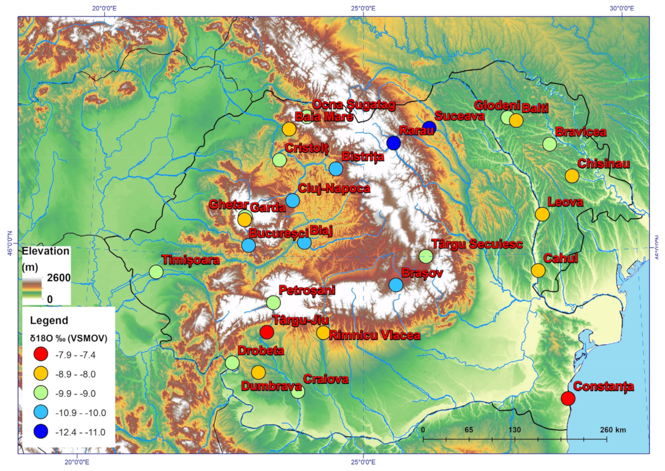
To provide spatial and seasonal distribution of water isotopes and d-excess at the country level.
-
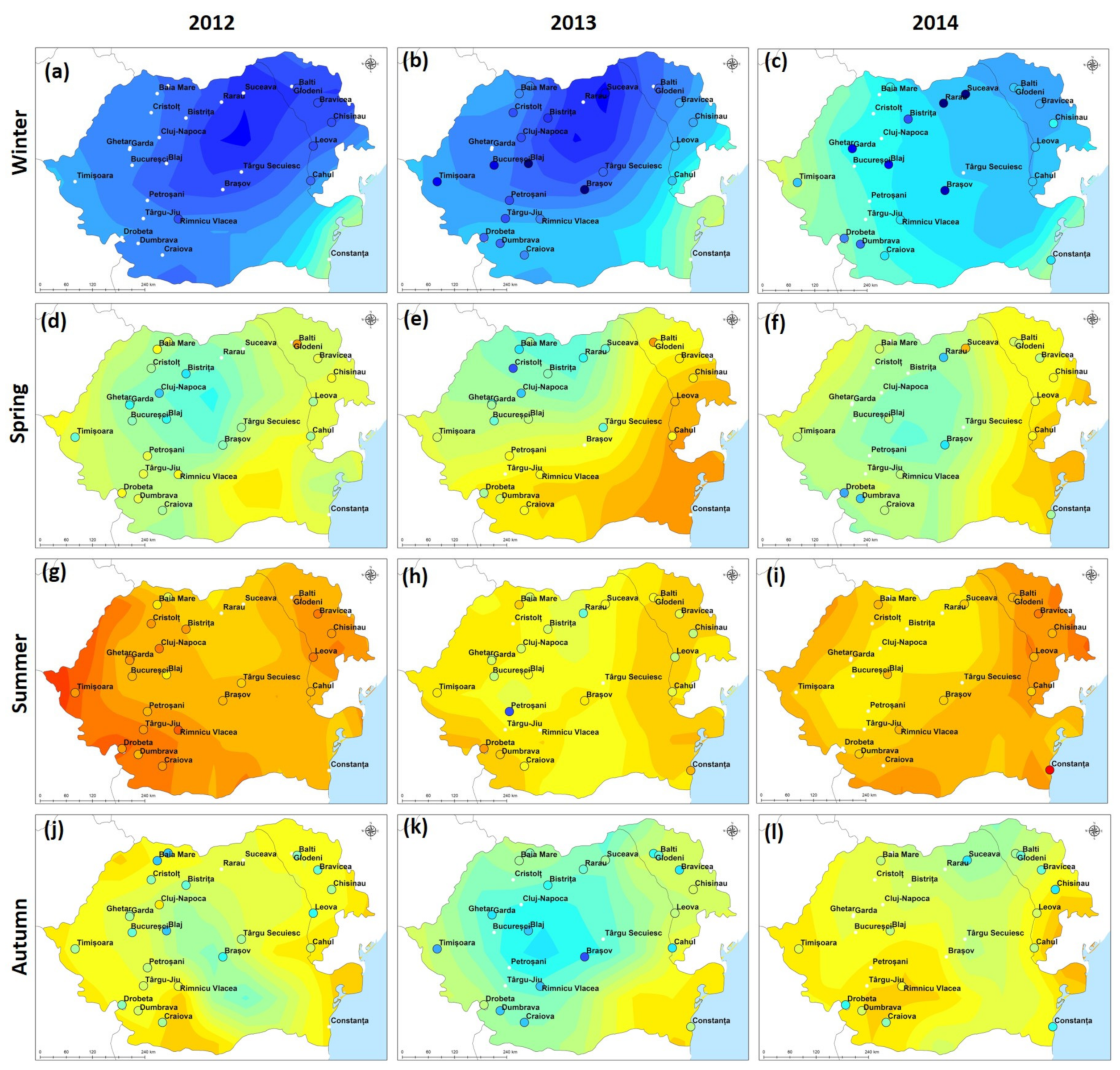
To construct the seasonal maps of the spatial distribution of the δ18O values in precipitation in Romania and the Republic of Moldova.
-
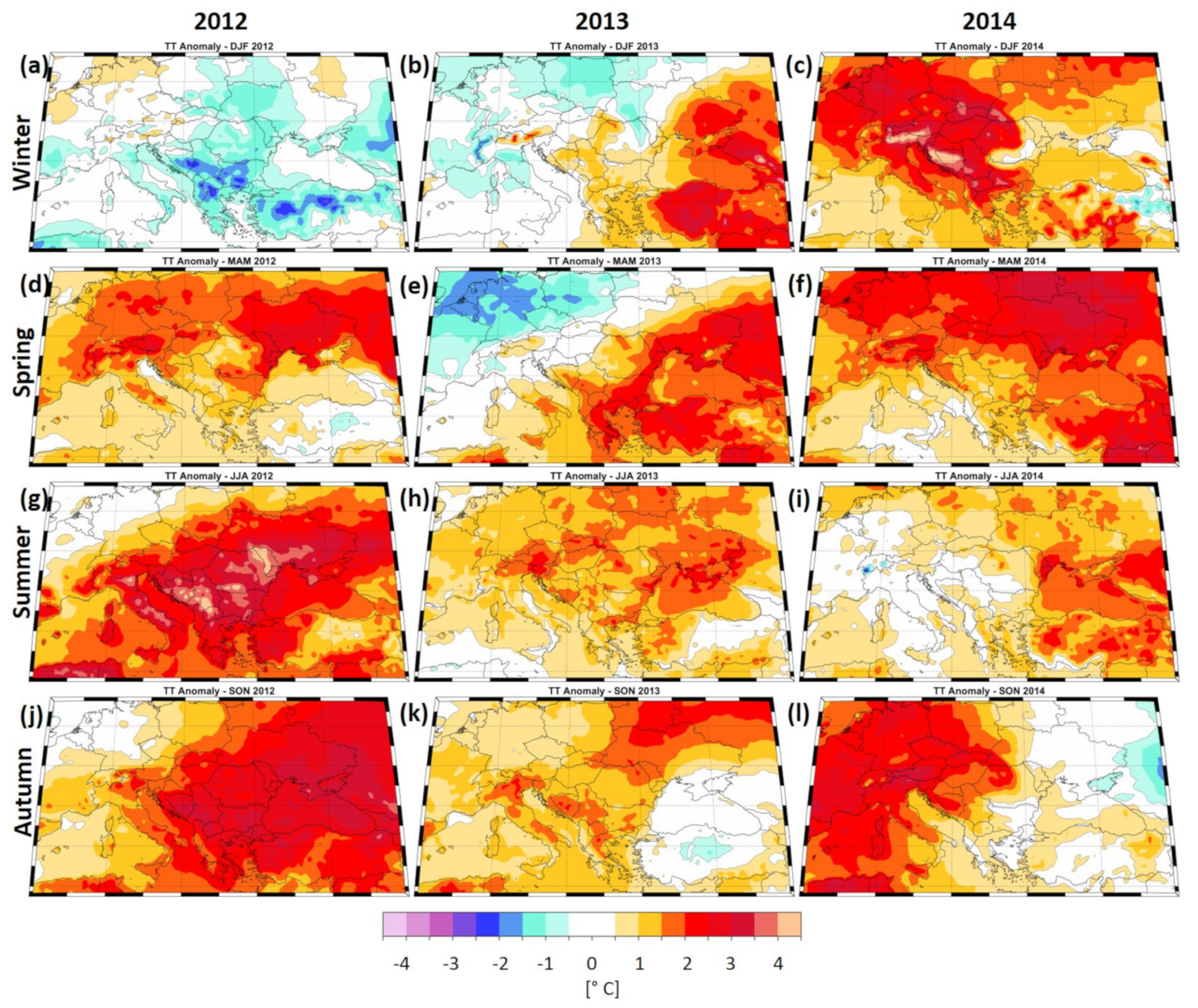
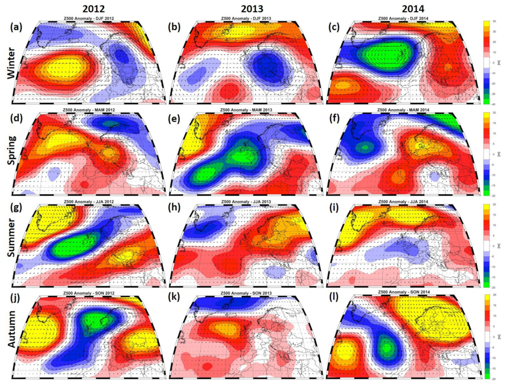
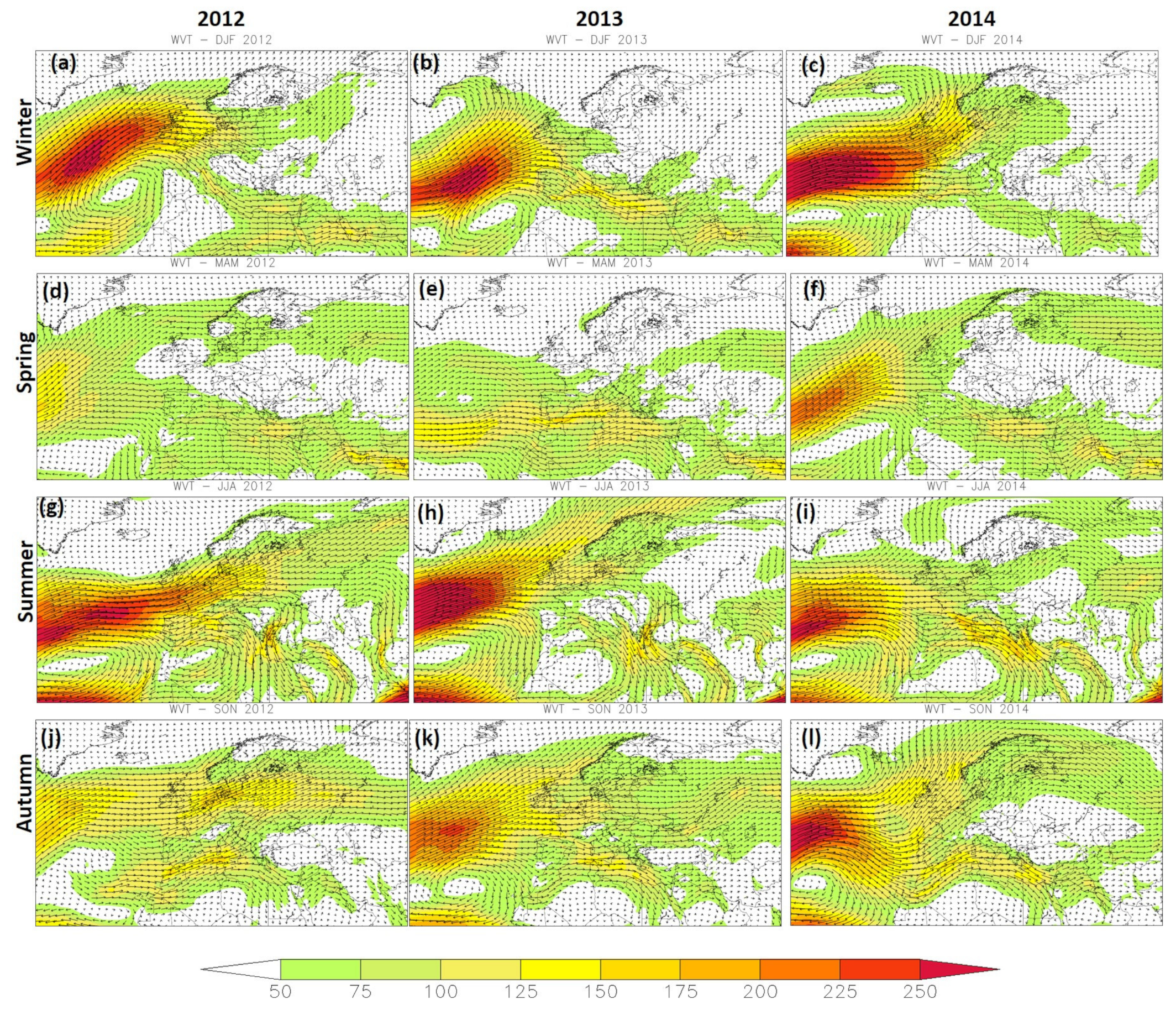
To investigate the influence of the large-scale atmospheric circulation on seasonal δ18O variability.
The presented results in this paper will enable access to observational measurements of the δ18O and δ2H from Romania and the Republic of Moldova, which can be applied to numerous hydroclimatic studies. Moreover, the seasonal maps of the spatial distribution of δ18O in precipitation for the analyzed area represent a novelty for the scientific community and were not available at this resolution until now.

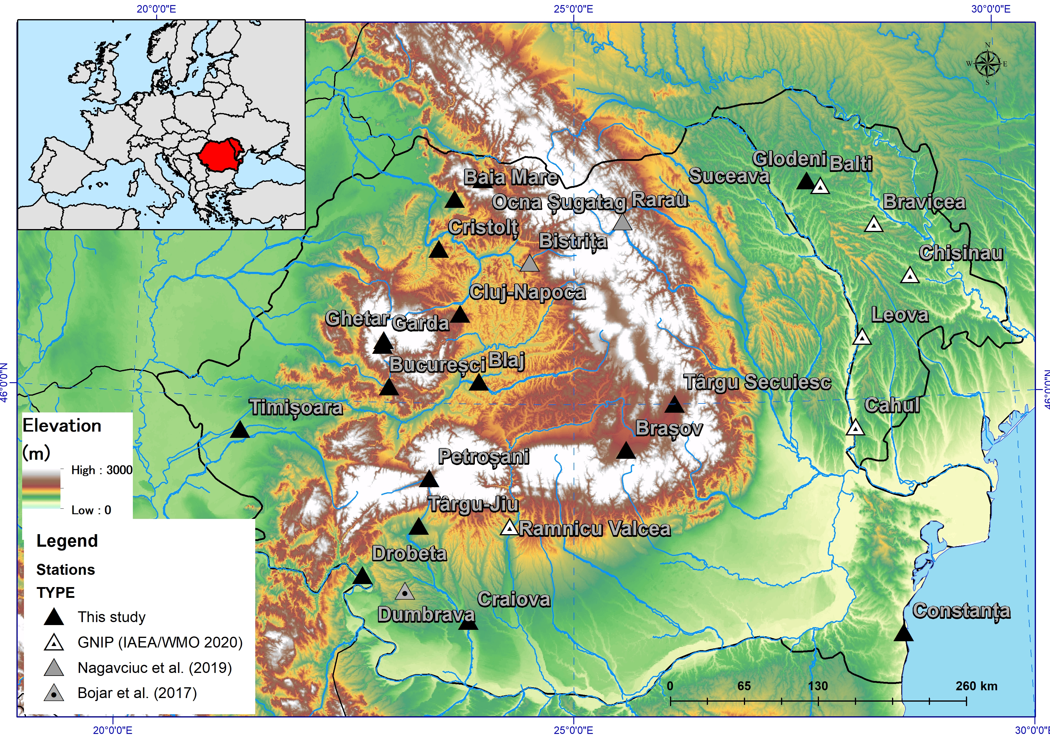
2. Materials and Methods

Between March 2012 and December 2014, monthly precipitation samples for stable isotopes at 17 stations in Romania and the Republic of Moldova (Figure 1, Table 1) were collected. The location of the stations was chosen to reflect the different climatic conditions in Romania (Figure 1) and also to span the largest latitudinal (2°30′), longitudinal (6°30′), and altitudinal (1500 m) gradients.
Table 1. The names of the study sites for measurement samples, with the corresponding abbreviations, country, coordinates, elevations, analyzed periods, and the data sources.
NRStation NameAbbreviationCountryLatitudeLongitudeAltitude (m. a.s.l.)Analyzed PeriodStudy/Reference
1Baia MareBMRomania47°37′8.86″ N23°36′21.42″ E284March 2012–December 2014This study
2BlajBJRomania46°10′42.67″ N23°55′11.99″ E257March 2012–December 2014This study
3BrașovBVRomania45°39′27.56″ N25°34′51.59″ E555April 2012–July 2014This study
4BucureșciBURomania46°7′37.56″ N22°53′53.64″ E320April 2012–June 2013This study
5Cluj NapocaCJRomania46°42′41.67″ N23°41′33.58″ E362March 2012–July 2013This study
6ConstanțaCTRomania44°8′33.00″ N28°37′17.00″ E35June 2013–November 2014This study
7CraiovaCRRomania44°17′5.40″ N23°50′19.45″ E112March 2012–December 2014This study
8CristolțCTRomania47°13′20.94″ N23°26′2.82″ E296March 2012–March 2013This study
9Drobeta Turnu SeverinDTSRomania44°37′42.87″ N22°39′38.01″ E62March 2012–December 2014This study
10GârdaGDRomania46°27′47.67″ N22°49′28.48″ E747March 2012–June 2013This study
11GhețarCHRomania46°29′28.45″ N22°49′26.02″ E1101March 2012–December 2013Bădăluță et al. (2020) [27]
12GlodeniGLRep. Moldova47°44′30.37″ N27°43′27.03″ E150May 2013–December 2014This study
13Ocna ȘugatagOSRomania47°46′53.41″ N23°56′22.18″ E495March 2012–December 2013This study
14PetroșaniPTRomania45°24′49.21″ N23°22′0.10″ E603May 2012–July 2013This study
15Târgu SecuiescTgSRomania46°0′10.46″ N26°8′31.29″ E567April 2012–April 2013This study
16Târgu-JiuTgJRomania45°2′1.70″ N23°16′32.91″ E204March 2012–December 2012This study
17TimișoaraTMRomania45°44′48.90″ N21°13′50.37″ E90March 2012–December 2014This study
18BistrițaBNRomania47°7′20.59″ N24°29′25.23″ E400March 2012–January 2014Nagavciuc et al. (2019) [22]
19SuceavaSVRomania47°37′00.00″ N26°13′59.99″ E350March 2012–December 2014Nagavciuc et al. (2019) [22]
20RarauRARomania47°27′00.0″ N25°33′59.99″ E1600March 2012–December 2014Nagavciuc et al. (2019) [22]
21Ramnicu ValceaRVRomania45°02′07.00″ N24°17′3.00″ E237January 2012–December 2014GNIP [3]
22BaltiBLRep. Moldova47°42′00.00″ N27°52′59.99″ E231January 2012–December 2014GNIP [3]
23BraviceaBRRep. Moldova47°24′00.00″ N28°29′29.97″ E78January 2012–December 2014GNIP [3]
24CahulCARep. Moldova45°47′59.99″ N28°11′59.99″ E113January 2012–December 2014GNIP [3]
25ChișinăuCHRep. Moldova46°57′59.99″ N28°54′00.00″ E125January 2012–December 2014GNIP [3]
26LeovaLERep. Moldova46°29′49.99″ N28°18′00.00″ E156January 2012–December 2014GNIP [3]
27DumbravaDURomania44°31′0.00″ N23°7′59.99″ E335April 2012–November 2014Bojar et al. (2017) [21]
The water was collected continuously using tube-dip-in 5 L water collectors [28]. At the end of each month, a 22 mL aliquot was collected from the container and stored (in HDPE scintillation vials) at 4 °C. In winter, snowfall samples were collected in 10 L (40 cm deep) plastic containers, allowed to melt at room temperature at the end of each month, and stored similarly to the liquid water samples [16]. Water samples were analyzed for their stable isotopic composition at the Stable Isotope Laboratory, Ștefan cel Mare University (Suceava), using a Picarro L2130-i CRDS analyzer coupled with a high-precision vaporizing module. Prior to analyses, the samples were filtered through 0.45 μm nylon membranes. Each sample was manually injected into the vaporization module between 6 and 20 times, and the last four injections were used for further processing [23]. The raw values were normalized on the SMOW-SLAP scale using two internal standards calibrated against the primary VSMOW2 and SLAP2 standards provided by IAEA. The stable isotope values are reported using the standard δ (delta) notation. On the basis of the repeated measurements of an internal standard, the precision of the measurements is estimated to be better than 0.16‰ for δ18O and 0.7‰ for δ2H, respectively.
Besides these 17 stations, for the discussion of our results, we combined our dataset with data from the other 10 stations (Table 1) that were previously published, either by our group [22,23,25] or others [10,24,29,30].
Meteorological data (monthly average air temperature and precipitation amount) were provided by the National Meteorological Administration. The meteorological stations are located <2 km from the collection site and at the same altitude (within 10 m). At Cristolț, we measured the air temperature using a calibrated Gemini TinyTag 2 datalogger (0.5 °C accuracy and 0.01 °C resolution at 0 °C). For Ghețar, we used the meteorological data from Stâna de Vale station, located 25 km NNW from the sampling site, at the same altitude and with similar exposure to the main wind directions (west).
The modeled stable oxygen and hydrogen water isotopes are based on the ECHAM5-wiso model, which is an isotope-enabled atmospheric circulation model [17,26,31]. ECHAM-wiso was developed by implementing δ18O in the hydrological cycle of an atmospheric general circulation model (ECHAM5), developed at the Max Planck Institute for Meteorology [31]. The ECHAM5-wiso model results are consistent with the annual and seasonal observations from GNIP data both globally and at the European level [25,26]. The spatial resolution of the model is 0.75° × 0.75° (T159) and covers the period 1979–2018 [26]. For the current study, we used the simulated monthly data of δ18O water from January 2012 to December 2014.
In order to analyze the relationship between the variability of the stable isotopes in precipitation and the large-scale circulation patterns, we computed the seasonal anomalies (i.e., December–January–February (DJF), March–April–May (MAM), June–July–August (JJA), and September–October–November (SON)) of the geopotential height at 500 mb (Z500), the vertically integrated water vapor transport (WVT), mean air temperature, and monthly precipitation over the period 2012–2014. The Z500 field was extracted from the ERA5 reanalysis project [32] and has a spatial resolution of 0.25° × 0.25°, covering the 1950–2021 period. The vertically integrated water vapor transport (WVT) [33] was calculated through the zonal wind (u), meridional wind (v), and specific humidity (q) from the ERA5 Reanalysis data [32]. The mean air temperature and the monthly precipitation amount were extracted from the EOBS-v20e dataset [34].
We determined local meteoric water lines (LMWL), defined as δ2H = a * δ18O + b [35], at 17 stations that were chosen in such a way to have at least one-year long time series of δ18O and δ2H. The “method of choice” in determining LMWLs is the ordinary least squares regression (OLSR) method [35], a method that does not account for the amount of precipitation (e.g., [36]). However, in summer, secondary (sub-cloud) evaporation of the falling raindrops results in low deuterium excess values in precipitation, while prolonged precipitation events tend to be depleted in the heavy (18O and 2H) isotopes (e.g., [4]). Thus, in summer, rain events in areas with low precipitation amounts and high air temperatures result in low amounts of water with very low d-excess, while prolonged (several days) rain events are associated with generally low air temperatures (e.g., in spring and autumn), resulting in large amounts of water with lower δ18O and δ2H values than expected from temperature influence only. The results are that the slope and intercept of the LMWL are heavily influenced by these conditions, further affecting the understanding of hydrological processes and interpretation of stable isotope-based proxies in paleoclimate studies. To overcome these issues, Hughes and Crawford [36] developed a novel method to determine the LMWL, which considers both the δ18O and δ2H and the amount of precipitation. This method, termed precipitation amount weighted least squares regression (PWLSR), aims to mitigate the bias induced by post-precipitation processes.

3. Results and Discussions

The main characteristics of the stable isotope data are shown in Table 1, and the full dataset will be available in the GNIP database.

3.1. Local Meteoric Water Lines

We determined the LMWLs for our study sites and for the stations previously published, and the results are shown in Table S1. Regardless of the method used (OLSR or PWLSR), the slopes and intercepts are close to the GMWL, defined either as δ2H = 8 * δ18O + 10 by Craig (1961) [2] or as δ2H = 8.2 * δ18O + 11.27 [5]. Stations in western and northern Romania, influenced by the westerly winds carrying moisture from the Atlantic Ocean, tend to have LMWLS with higher values of the slopes (between 7.7 and 8.14) and intercepts (between 7.46 and 13.72), whereas those in SW Romania, with a sub-Mediterranean climate, have both lower slopes (between 7.06 and 7.70) and intercepts (between 3.75 and 8.77) (Figure 2). Similarly, sites in central and eastern Romania have lower slopes and intercepts, likely indicating the influence of evaporation on raindrops during hot and dry summers [37,38,39]. At most stations, the PWLSR method resulted in higher slopes (9 out of 16) and intercepts (12 out of 16), indicating that the bias induced by sub-cloud evaporation mostly affects the intercept of the LMWL and not the slope (Table S1). The differences in slopes and intercepts are higher at stations located in the sub-Mediterranean climate (e.g., DTS and DU, located within 20 km of each other). A similar increase in LMWL slope and intercept by using PWSLR over OLSR has been found by Hughes and Crawford [36] at Mediterranean stations, likely triggered by evaporation under hot and dry summer weather conditions. Stations with lower slopes (but variable intercepts) are located in central and northern Romania, where winter precipitation contributes more than the average amounts of water in the annual balance.
These findings again mirror those found by Hughes and Crawford [36]. When analyzing global patterns, these authors identified central Europe as a region where the choice of PWSLR over OLSR results in LMWLs with lower slopes. Overall, there seems to be a tendency towards larger differences with a lower number of samples (e.g., Rarău, TGS), potentially suggesting that monitoring over longer time periods might erase the bias induced by post-precipitation (or post-depositional) processes (e.g., sub-cloud evaporation or evaporation in the collecting devices).
As these LMWLs are defined on the basis of a limited time series of δ18O and δ2H determinations in precipitation water, we wish to emphasize their preliminary character. The sensitivity of δ18O-δ2H covariance to the length of the analyzed period (e.g., Putman et al., 2019 [40]) suggests that longer observation periods might result in (slightly) different values for the slopes and intercepts of the LMWLs, which could potentially affect subsequent paleoclimate and hydrological studies.

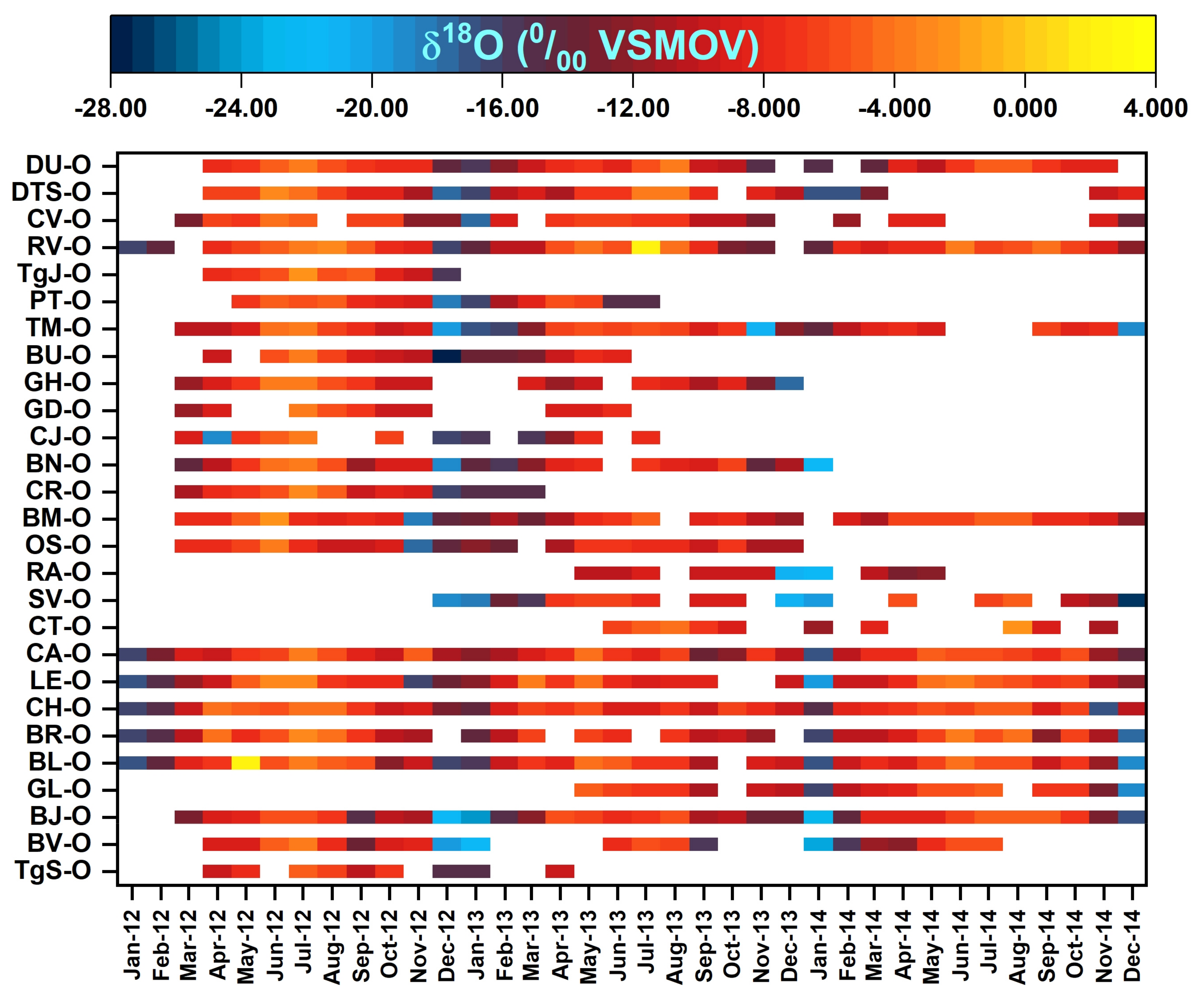
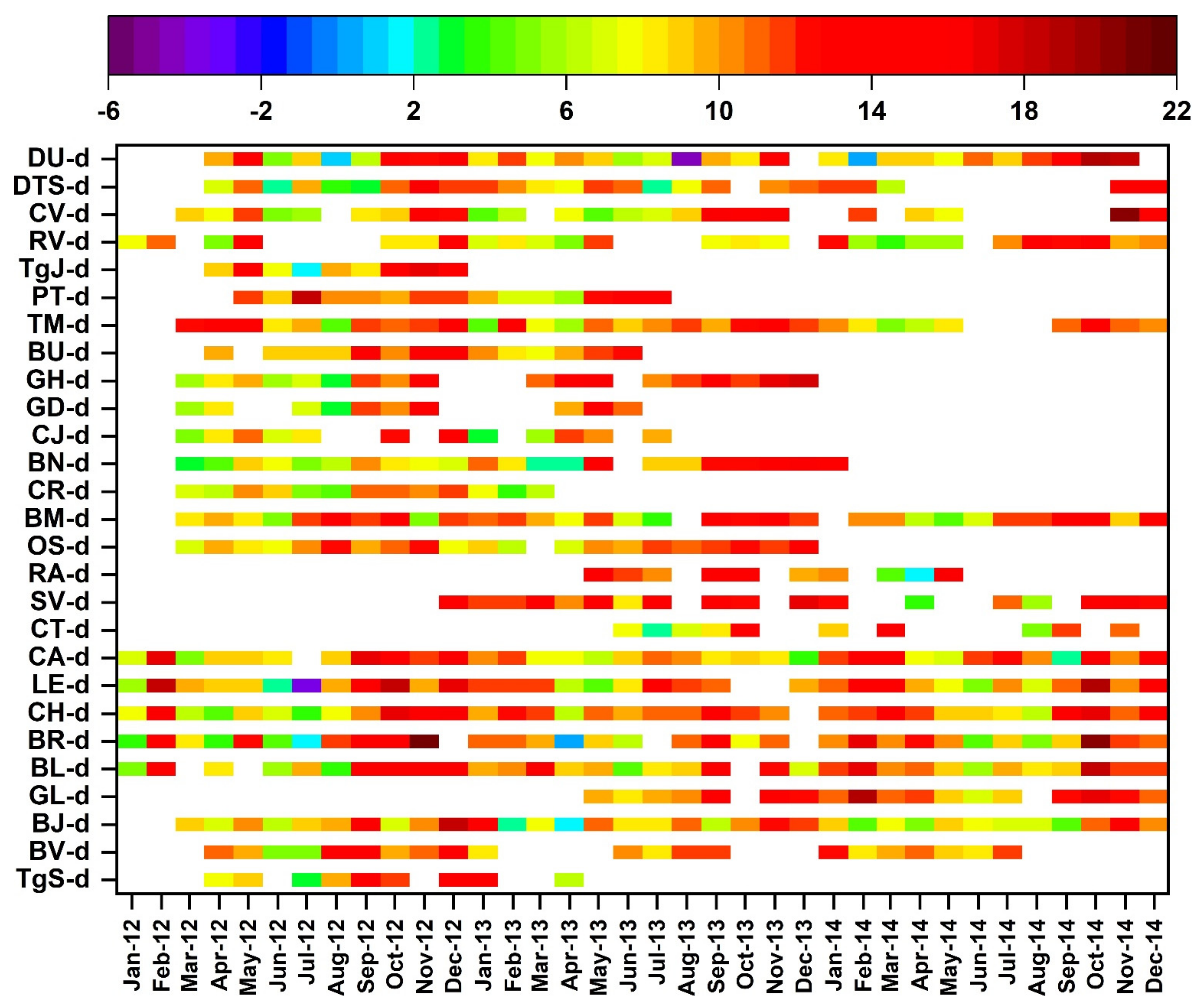
3.2. Temporal Variability of δ18O, δ2H, and D-Excess

The temporal variation of stable δ18O and δ2H composition of precipitation throughout Romania during the monitoring period from March 2012 to December 2014 are presented in Figure 3 and Figure S1. The δ18O values vary between −27.9‰ (i.e., December 2014 at Suceava station) and −2.4‰ (i.e., August 2014 at CT station), while the δ2H values vary between −209‰ (i.e., December 2012 at Bucuresti station) and −14‰ (i.e., August 2014 at CT station). The monthly variation of the δ18O and δ2H shows a clearly interannual variation, with distinct seasonal differences, with the higher values during the summer and the lowest values during the winter. Generally, their variability reflects the variation of the temperature and precipitation [4,41]. During the summer season, the δ18O values have a lower variability between the analyzed stations, with a mean standard deviation of 1.5 (and ranging from 0.6 to 3.3), compared with the winter season, when the mean standard deviation is 3.6 (and ranging from 2.3 to 5.9). Similar results were found for δ2H variations. These seasonal differences can be explained by different sources of air moisture reaching the study area in winter, compared to more uniform ones in summer (likely convective rains locally recycling moisture) [42].
The mean d-excess was 9.7‰ and varied in the range of −31.2‰ (i.e., May 2012 at Balti station) up to 22.2‰ (i.e., November 2013 at Rarau station). Even the monthly d-excess values are equitably distributed relatively to the mean (50% of obtained values are below 10‰ which is the global average). The lowest d-excess values have occurred mostly during the summer season (average = 7.8‰), which can be explained by secondary evaporation during rainfall [1], while the highest values occurred mainly during the autumn season (average 11.9‰) indicating moisture sources derived from highly evaporated seas to the south (Mediterranean Sea) and East (Black Sea) of the study area [5].
The stable isotope composition of precipitation in January 2012 had very low δ18O values (around −16.5‰) at stations from the Republic of Moldova and RV station. In February 2012, the δ18O increased up to −14.5‰, and up to −11‰ in March 2012, except at the OS and BM stations, where the δ18O values registered values of −7.7‰. In April 2012, δ18O values presented a higher variability among stations, with higher δ18O values (~−7.7‰) in the north-eastern part (at BL, BR, CH, and LE stations) and south-western part (at TgJ, RV, CV, DTS, and DU stations), and lower δ18O values (around −10‰) in the central part (at TgS, BV, and BJ stations), western part (at BN, GD, GH, BU, and TM stations), and south-eastern part (at LE and CA stations), with an extreme value at CJ station (−18.8‰). In May 2012, the increasing trend remained constant at all stations. The increasing trend continued until the June–July period when the highest δ18O (−4.5‰) values were recorded. In August 2012, the δ18O values remained similar to the previous months, while the lowest values were recorded at BM and OS stations (−9.4‰ and −8.2‰, respectively). From September 2012, a decreasing trend can be observed, with lower δ18O values (~−11‰) in the central part (at TgS, BV, and BJ stations), and in the north and north-western part (at OS, BM, CR, and BN stations), while in the rest of the stations, the δ18O values remain similar to August values. In October 2012, the highest δ18O values remained in the south-western part (at TgS, RV, CV, DTS, and DU stations). The slowly decreasing trend is characteristic also for November 2012, with extremely low δ18O values at LE, OS, and BM stations (≈17.5‰). In December 2012, the δ18O values dropped to ≈16‰ at all stations, while at some stations, the δ18O values were less than −20‰ (e.g., BU and BJ).
During January 2013, the low δ18O values were maintained. In February 2013, in the central (at BJ station), north (at SV and OS station), and western parts (at BM, BN, BU, and TM station), the δ18O values were around −14‰, while in the eastern part (at RV, CR, and DTS), higher δ18O values were recorded, around −10‰. In March 2013, the eastern part was characterized by higher δ18O values (~6.5‰), while at the other stations, the δ18O values remained lower (≈12‰). A similar trend was maintained during April 2013. In May 2013, there was a sharp increase at most stations, reaching average values of −6.5‰. The mean δ18O values in June and July 2013 were around −7‰, except at the PT station, where the δ18O values were around −15‰. In August, δ18O values were similar to values recorded in May 2013. Since September, the δ18O values started to decrease, with mean values of −10‰, and remained at this level also during October, November, and December 2013, but also reached much lower values at some stations (e.g., δ18O in November 2013 at TM station = −20.9‰ or SV and RA in December 2013 = −21.2 and −20.7‰, respectively).
In January 2014, the annual minimum was recorded, with δ18O values lower than −14‰, except CT station, where δ18O was −11.5‰. Since February 2014, the δ18O values started to decrease and reached an average of −10‰ on March 2014, while at DTS, DU, and BV stations, the δ18O values remained similar to February 2014 values. A similar trend was observed in April 2014. In May 2014, the δ18O values were around −7.5‰ and continued to decrease during the summer months, while in August 2014, the maximum peak was reached, with the mean value of −5‰. In September 2014, δ18O values started to decrease, and the mean δ18O value was −7.7‰. Similar values were recorded in October 2014. In November 2014, the δ18O values dropped to −11‰, with lower values in the central and eastern parts and higher values in the west and south-western parts. In December 2014, very low δ18O values were recorded, up to −27.1‰ at the SV station.
The δ2H temporal variability was similar to that of δ18O variability (Figure S1), while the temporal variability of d-excess values presented particular differences (Figure 4 and Figure S2). During March and April 2012, the d-excess values were lower than 10, except at the TM station, while in May 2012, in the south-western part, the d-excess values exceeded 10 (DU, DTS, CV, RV, TgS, PT, and TM stations). In the summer 2012 months, d-excess values remained under 10, with a minimum in June (d-excess = 6.3), and presenting a slowly increasing trend (August mean d-excess = 7.7). This trend continued during the autumn months, with d-excess values higher than 10, reaching the maximum in December (mean d-excess = 13.8). In January 2013, at several stations, d-excess recorded an abrupt decrease. In February 2013, in the eastern and north parts, the d-excess exceeded 10, while in the western and southwestern parts, the d-excess values were below 10. A similar situation was found in March 2013. In April, except for CJ, GH, and DU, all other stations recorded d-excess values lower than 10. In May, in the eastern part, the d-excess remained under 10, while in the north and western parts, higher d-excess values were recorded. During summer 2013, the mean d-excess values were 9.3 and ranged from 2.3 in July at DTS to 13.8 in June and July at the PT station. The autumn 2013 months presented higher d-excess values, around 13 for almost all stations and months, with a maximum in November. Since December 2013, a decreasing trend can be observed and it was maintained in the following months until April 2014. In May 2014, the mean d-excess value was 8.6. Except for the CA station, during the summer 2014 months, the d-excess values remained under 10, while during the autumn 2014 months and December 2014, the d-excess values presented higher values, around ≈13.

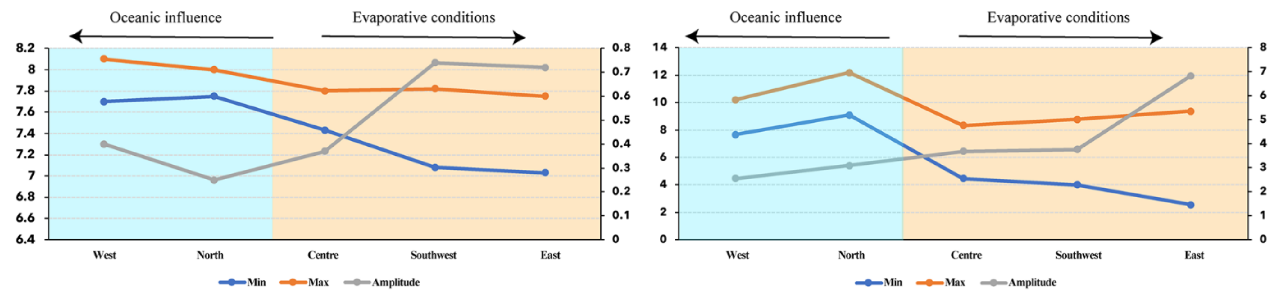
3.3. Temperature, Altitude, and Topographic Relationships

In order to determine the influence of the climate, orography, altitude, and geographical position on the stable isotope composition of precipitation, we analyzed the variability of the δ18O values in relationship with different parameters, namely, the monthly mean temperature, precipitation, altitude, and geographical (orthographical) position.
The monthly isotopic composition of Romanian precipitation showed a clear annual cycle following the seasonal temperatures (Figure S3). The correlation between δ18O values and temperature at the analyzed stations varied between 0.52 at PT and 0.95 at TgG, with an average of 0.8, confirming once again that temperature is one of the principal factors that controls the water isotopic composition in precipitation [2,4]. Similar results were found for the relationship between δ2H values and temperature, with a mean correlation coefficient of 0.76.
The altitudinal range of the analyzed stations was 1565 m and varied between 35 m (CT station) and 1600 m (RA station). Taking into account the uneven distribution of analyzed stations by altitude categories (17 from 28 stations have altitudes between 100 and 500 m, and only 2 stations have altitudes over 1000 m) and by the Carpathian position and orography, it is difficult to summarize the altitude effect over the analyzed region on the basis of the available data. Nevertheless, we found a significant negative correlation between mean δ18O values for the 2012–2014 period and altitude (r = −0.47), with an average altitude gradient of 0.17‰/100 m for δ18O. The obtained altitude gradient was lower than the gradient found by Bădăluță et al. [23] in a small region in the northern part of the study area, but this difference can be explained by the different number of stations and the analyzed area.
The Carpathian Mountains, through their geographical position and orographical characteristics, strongly influence the variability of the stable isotopes in precipitation in Romania [25]. The lowest mean δ18O values (less than −12‰) were recorded at RA—the station with the higher altitude (1600 m), and the SV station situated in the northern part of the Carpathian, near the RA station (Figure 5). In the inner part of the Carpathian chain, the δ18O values varied between −10‰ and −11% (BN, CJ, BU, BJ, and BV), while in the outer part of the Carpathian chain, the δ18O values oscillated between −8‰ and −10‰, with the higher δ18O values at CT—the station with the lowest altitude (35 m) situated near the Black Sea, and TgS—the station located in a mountain depression. The uneven distribution of the δ18O values with latitudinal, longitudinal, and altitudinal gradients can be given by complex local orography with high peaks, mountain depressions, and lowlands, which indicate the importance of the local re-evaporation in the monthly variation of δ18O in precipitation in Romania and the Republic of Moldova. Our results based on the observation data are in agreement with the findings of Nagavciuc et al. [25], who indicated that in the extra-Carpathian regions, the mean δ18O values are much higher compared with those in the inter-Carpathian and Carpathian regions, and the local re-evaporation acts as an important contributor to the increased δ18O values in the extra-Carpathian regions, on the basis of the simulated data over the same region.

3.4. Spatial Variability of δ18O, δ2H, and D-Excess and Large-Scale Atmospheric Circulation

The analysis of the spatial distribution of stable isotopes in precipitation water, presented in the previous section, provides an overall picture of the variability of the mean seasonal oxygen isotope composition of precipitation in Romania and the Republic of Moldova over the 2012–2014 period. In order to have a better overview of the spatial variability of the δ18O, δ2H, and d-excess, besides the measured data, we also used the stable oxygen and hydrogen water isotopes as obtained from the ECHAM5-wiso model [17,26], which showed that they overall are in good agreement with the observational isotopic data for this region [25]. Furthermore, to show both the origin of the air moisture and the interaction with regional and local patterns, we analyzed the link between the spatial δ18O variations and the large-scale circulation patterns on a seasonal scale.
On the basis of the observed values, winter 2012 was characterized by very low δ18O values at the country level. The lowest values (up to −18‰) were recorded over the central and north-eastern parts of Romania and the northern part of the Republic of Moldova. Only over the Romanian Black Sea coastline did the δ18O values have higher values, up to −10‰ (Figure 6a). This spatial pattern observed in the seasonal values of δ18O was occurring in conditions of negative temperature anomalies over Romania and the Republic of Moldova (Figure 7a) generated by a low-pressure system over Europe and a high-pressure system over the Atlantic Ocean (Figure 8a), which favored the advection of the cold and wet air masses from the Atlantic Ocean over Europe, including our study area (Figure 9a). Winter 2013 had similar spatial variability of δ18O values as winter 2012 (Figure 6b), but with weak positive temperature anomalies in the western and southern parts of Romania and negative temperature anomalies in the north-eastern parts (Figure 7b). A strong negative low-pressure system prevailed over Europe during the winter of 2013 (Figure 8b), favoring the advection of cold and wet air masses from the Atlantic Ocean over Europe (Figure 9b), including our study area. Compared to the 2012 and 2013 winters, winter 2014 was characterized by higher δ18O values, with low δ18O values in the eastern part of Romania and higher δ18O values in the western part (Figure 6c). Strong positive temperature anomalies can explain this distribution in the intra-Carpathian region and very weak positive temperature anomalies in the extra-Carpathian region (Figure 7c). These conditions were developing under the influence of a strong high-pressure system over Europe (Figure 8c), which favored the advection of the warm and wet air masses from the Atlantic Ocean over Europe via the Mediterranean region (Figure 9c).
Looking at the spring season, the lowest δ18O values in Spring 2012 were recorded in the central part of Romania, while higher δ18O were recorded in the western and south-eastern parts (Figure 6d). This spatial pattern can be explained through the week positive temperature anomalies in the intra-Carpathian region and strong positive temperature anomalies in the extra-Carpathian region (Figure 7d), preceded by a high-pressure system over Europe, with the center over Germany (Figure 8d), which favored the deflection of the storm tracks either towards Fennoscandia or over the Mediterranean Sea (Figure 9d). Low δ18O values characterized the spatial distribution of the δ18O in the spring of 2013 in north-western Romania, and there was high δ18O in the south-eastern part (e.g., over the Dobrogea region) (Figure 6e), reflecting the temperature spatial distribution with positive temperature anomalies centralized over the Dobrogea region (Figure 7e). These conditions were the results of the high-pressure system over the Black Sea and a low-pressure system over the Atlantic Ocean and western Europe (Figure 8e). This pattern allowed the advection of the moist air masses from the Mediterranean Sea to Romania (Figure 9e), which in turn led to high δ18O, especially over the south-eastern part of Romania.
The mean δ18O values in spring 2014 were similar to the ones recorded in 2012 and 2013, with the lowest values in the central part of Romania and the highest δ18O values in the eastern part of the study area (Figure 6f). Spring 2014 was also characterized by positive temperature anomalies over the eastern part of the study area (Figure 7f). The large-scale atmospheric circulation was characterized by a high-pressure system focused on the North Sea, a strong low-pressure system over the Atlantic Ocean, and a weak low-pressure system over the eastern Mediterranean Sea (Figure 8f) that defected the storm track towards the Fennoscandia and the Mediterranean Sea (Figure 9f).
Summer 2012 was characterized by the highest δ18O values over the analyzed period. The highest values (around −3‰) were recorded in the western and south-western parts of Romania, while the lowest values (around −6‰) were recorded in the northern part of Romania (Figure 6g). The summer of 2012 was characterized by very strong positive temperature anomalies (Figure 7g), with extreme heatwaves and dry spells [39]. These conditions were established due to a high-pressure system centered over Romania and a low-pressure system over the Atlantic Ocean (Figure 8g), which favored the advection of the hot and dry air over Romania (Figure 9g). In the summer of 2013, the δ18O values varied between −7‰ and −5‰, with the highest δ18O values in the central part (Figure 6h), a region where the highest temperature anomalies for this season were recorded (Figure 7h). These conditions were developed under the influence of a high-pressure system over central-northern Europe and a low-pressure system over the Mediterranean Sea (Figure 8h). In the summer of 2014, the δ18O values ranged from around −7‰ to −4‰, with the lowest values in the central part of Romania (Figure 6i), corroborated with positive temperature anomalies (Figure 7i). In the summer of 2014, a high-pressure system was prevailing over the northern part of Europe and the Atlantic Ocean, and a low-pressure system was active over the western part of Europe and the southern Atlantic Ocean (Figure 8i), which deflected the storm tracks from the Atlantic Ocean towards our analyzed area (Figure 9i).
In Autumn 2012, the lowest δ18O values (−10‰) were recorded in the central and southern parts of Romania, increasing up to −5‰ in the periphery of the analyzed area (Figure 6j). This spatial distribution can be explained by the strong co-occurrence of positive temperature anomalies over the analyzed region, which were generated by a high-pressure system centered over eastern Europe and a low-pressure system over the northern Atlantic Ocean (Figure 7j and Figure 8j). As a result, the spatial structure of the large-scale circulation (Figure 8j) favored the advection of the warm and wet air masses from the Mediterranean Sea over Romania (Figure 9j). In autumn 2013, the lowest δ18O values reached −11‰ in the central part of Romania, while the highest δ18O values (−5‰) were recorded in the south-eastern part of Romania (Figure 6k). The 2013 autumn was characterized by weak positive temperature anomalies over Europe (Figure 7k), mainly imposed by a high-pressure system over the Atlantic Ocean extending up to Europe (Figure 8k). This pattern favored the advection of wet air from the Atlantic Ocean over Romania (Figure 9k), thus leading to high δ18O at almost all analyzed stations. In the autumn of 2014, the δ18O values varied between −9‰ in the north-eastern part of Romania and –5‰ in the western and south-eastern parts of Romania (Figure 6l). This dipole-like structure in the observed δ18O values can be also observed in the spatial distribution of temperature anomalies (Figure 7l). The highest positive temperature anomalies were recorded in the intra-Carpathian region (Figure 7l) and were mainly driven by the persistence of a high-pressure system over the north and western part of Europe and a low-pressure system over the Atlantic Ocean (Figure 8l). This pattern favored the advection of the dry air masses from the Atlantic Ocean over the intra-Carpathian region and the wet air masses from the Mediterranean Sea over the extra-Carpathian region (Figure 9l).

4. Conclusions

Here, we presented the first high-resolution seasonal maps of the spatio-temporal distribution of δ18O values in precipitation in Romania and the Republic of Moldova, according to observational and simulated data. According to our results, the slope and intercept of the LMWLS at the stations situated in the western and northern parts of Romania tended to have higher values than those of the LMWLS at stations situated in the south-western parts of Romania. The monthly variation of the δ18O and δ2H showed a clearly interannual variation, with distinct seasonal differences, following the seasonal temperatures. Even the monthly d-excess values were equitably distributed reported to the mean (50% of obtained values are below 10‰ which is the global average), and mostly the lowest d-excess values occurred during the summer season (average = 7.8‰), while mostly the highest values occurred during the autumn season (average 11.9‰). The Carpathian Mountains through their geographical and orographical position strongly influence the variability of the stable isotopes in precipitation. The δ18O values in the inner part of the Carpathian chain were lower than the δ18O values in the outer part of the Carpathian chain, while the higher δ18O values were recorded at CT, the station with the lowest altitude (35 m) situated near the Black Sea.
The analysis of the spatial distribution of stable isotopes in precipitation water was made on the basis of both observational data and model ECHAM5-wiso data. This allowed us to study the origin of the air moisture and the interaction with regional and local patterns and to analyze the link between the spatial δ18O variations and the large-scale circulation patterns on a seasonal scale. The spatio-temporal distribution of δ18O values over the Carpathian Mountains revealed significant differences, mainly owing to their particular orography.
The seasonal large-scale patterns associated with the variability of our δ18O network revealed that low δ18O values in winter are associated with negative temperature anomalies over Romania and the Republic of Moldova, which usually are generated by a low-pressure system over Europe and a high-pressure system over the Atlantic Ocean that favors the advection of the cold and wet air masses from the Atlantic Ocean over Europe. On the contrary, high δ18O values in summer are associated with strong positive temperature anomalies, with extreme heatwaves and dry spells. These conditions are established due to a prevalence of a high-pressure system centered over Romania and a low-pressure system over the Atlantic Ocean, which usually favors the advection of the hot and dry air over Romania. In this respect, the observed relationship between δ18O variation and temperature has emphasized the large-scale atmospheric circulation patterns’ role in precipitation δ18O variability. The persistence and prevalence of different seasonal large-scale atmospheric patterns lead to the advection of different air masses, influencing the regional temperature and, therefore the δ18O values in precipitation.
The combination of both observational and modeled data revealed that in general, the simulated δ18O values reflected with accuracy the spatio-temporal variability. Still, they tended to underestimate the δ18O values compared to measured δ18O data, emphasizing once again the necessity of the local studies that will help to improve the resolution of the simulated data. We argue that the performed analysis of the stable isotopes in water precipitation from Romania and the Republic of Moldova can help in establishing the stable isotope framework in the wider Carpathian Region, a region that is still very poorly represented in the GNIP database.

Supplementary Materials

The following supporting information can be downloaded at https://www.mdpi.com/article/10.3390/w14162547/s1, Figure S1: The temporal variation of stable δ2H at the analyzed stations for the January 2012 – December 2014 period; Figure S2: Seasoal spatial distribution of the mean d-excess values in Romania and the Republic of Moldova, for the January 2012 – December 2014 period; Figure S3: Measured monthly δ18O values in precipitation (blue line) and mean temperature (red line) for analysed period at Bistita, Baia Mare, Blaj, Brasov, Craiova, Drobeta Turnu Severin, Ghetar and Timisoara stations; Table S1: Local Meteoric Water Lines (LMWL) using ordinary least squares regression (OLSR) method, and precipitation amount weighted least squares regression (PWLSR) method, and the data sources, ds - differences in the slopes, di - differences in the intercepts.

Author Contributions

V.N., A.P. and M.I. conceptualized the study and wrote the original draft; V.N. and C.-A.B. measured the isotope data; O.B., S.B. (Sorin Bănică and Sandu Boengiu) and A.O. helped with data collection; M.-V.B. provided meteorological data. All authors helped write the paper. All authors have read and agreed to the published version of the manuscript.

Funding

The IAEA partly supported the stable isotope collection and analysis in the framework of CRP F33021 (Application and development of isotope techniques to evaluate human impacts on water balance and nutrient dynamics of large river basins, contract 18452/RO), CRP F31006 (Isotope variability of rain for assessing climate change impacts, contract 23550/RO), and RER 7013 contracts awarded to A.P. V.N. was supported by a grant of the Ministry of Research, Innovation and Digitization, CNCS/CCCDI–UEFISCDI, project number PN-III-P1-1.1-PD-2019-0469, within PNCDI III. M.I. was supported by Helmholtz Association through the joint program Changing Earth–Sustaining our Future (PoF IV) program of the AWI. Funding by the Helmholtz Climate Initiative REKLIM is gratefully acknowledged. C.-A.B. was supported by a grant of the Ministry of Research, Innovation and Digitization, CNCS/CCCDI–UEFISCDI, project number, PN-III-P1-1.1-PD-2021-0744, within PNCDI III. A.P. was supported by project PN-III-P2-2.1-PED-2019-410.

Data Availability Statement

The precipitation stable isotope data used in this study are openly available in the GNIP database or will be shortly made available after the publication. The data that support the findings of this study are openly available. The relevant papers associated with these datasets are referred in the text.

Acknowledgments

V.N.: I would like to thank my mom, Nagavciuc Zinaida, who collected monthly precipitation water samples for isotope measurements at Glodeni station for several years. We would like to thank Roman Elena for collecting monthly precipitation water samples at Constanta station. Moreover, we would like to thank all who helped with precipitation water collection (Marian Blănaru, Nicodim Pașca, Szőcs Mária, Anca Crăciunaș, Mircea Trif, Andrea Antonescu, Radu Antonescu, Aurelia Antonescu).

Conflicts of Interest

The authors declare no conflict of interest.

References

  1. Gat, J.R. Oxygen and Hydrogen Isotopes in the Hydrologic Cycle. Annu. Rev. Earth Planet. Sci. 1996, 24, 225–262. [Google Scholar] [CrossRef]
  2. Craig, H. Isotopic Variations in Meteoric Waters. Science 1961, 133, 1702–1703. [Google Scholar] [CrossRef] [PubMed]
  3. IAEA/WMO. Global Network of Isotopes in Precipitation. The GNIP Database. Available online: https://nucleus.iaea.org/wiser/index.aspx (accessed on 5 January 2020).
  4. Dansgaard, W. Stable isotopes in precipitation. Tellus 1964, 4, 436–468. [Google Scholar] [CrossRef]
  5. Rozanski, K.; Araguás-Araguás, L.; Gonfiantini, R. Isotopic Patterns in Modern Global Precipitation. J. Geophys. Res. 1992, 78, 1–36. [Google Scholar] [CrossRef]
  6. Araguas, L.; Danesi, P.; Froehlich, K.; Rozanski, K. Global Monitoring of the isotopic composition of precipitation. J. Radioanal. Nucl. Chem. 1996, 205, 189–200. [Google Scholar] [CrossRef]
  7. Langebroek, P.M.; Werner, M.; Lohmann, G. Climate information imprinted in oxygen-isotopic composition of precipitation in Europe. Earth Planet. Sci. Lett. 2011, 311, 144–154. [Google Scholar] [CrossRef]
  8. Wang, S.; Zhang, M.; Crawford, J.; Hughes, C.E.; Du, M.; Liu, X. The effect of moisture source and synoptic conditions on precipitation isotopes in arid central Asia. J. Geophys. Res. 2017, 122, 2667–2682. [Google Scholar] [CrossRef]
  9. Krklec, K.; Domínguez-Villar, D.; Lojen, S. The impact of moisture sources on the oxygen isotope composition of precipitation at a continental site in central Europe. J. Hydrol. 2018, 561, 810–821. [Google Scholar] [CrossRef]
  10. Bojar, A.V.; Ottner, F.; Bojar, H.P.; Grigorescu, D.; Perşoiu, A. Stable isotope and mineralogical investigations on clays from the Late Cretaceous sequences, Haţeg Basin, Romania. Appl. Clay Sci. 2009, 45, 155–163. [Google Scholar] [CrossRef]
  11. Verča, P.; Bronić, I.K.; Horvatinčić, N.; Barešić, J. Isotopic characteristics of precipitation in Slovenia and Croatia: Comparison of continental and maritime stations. J. Hydrol. 2006, 330, 457–469. [Google Scholar] [CrossRef]
  12. Gibson, J.J.; Fekete, B.M.; Bowen, G.J. Stable Isotopes in Large Scale Hydrological Applications. In Isoscapes: Understanding Movement Pattern and Process on Earth through Isotope Mapping; West, J.B., Bowen, G.J., Dawson, T.E., Tu, K.P., Eds.; Springer: Dordrecht, The Netherlands, 2010; pp. 389–405. ISBN 978-90-481-3354-3. [Google Scholar]
  13. Bowen, G.J.; Cerling, T.E.; Ehleringer, J.R.B.T.-T.E. Stable Isotopes and Human Water Resources: Signals of Change. In Stable Isotopes as Indicators of Ecological Change; Elsevier: Amsterdam, The Netherlands, 2007; Volume 1, pp. 283–300. ISBN 1936-7961. [Google Scholar]
  14. Coplen, T.B.; Herczeg, A.L.; Barnes, C. Isotope Engineering—Using Stable Isotopes of the Water Molecule to Solve Practical Problems. In Environmental Tracers in Subsurface Hydrology; Cook, P.G., Herczeg, A.L., Eds.; Springer: Boston, MA, USA, 2000; pp. 79–110. ISBN 978-1-4615-4557-6. [Google Scholar]
  15. Liu, Z.; Ma, F.; Hu, T.; Zhao, K.; Gao, T.; Zhao, H.; Ning, T. Using stable isotopes to quantify water uptake from different soil layers and water use efficiency of wheat under long-term tillage and straw return practices. Agric. Water Manag. 2020, 229, 105933. [Google Scholar] [CrossRef]
  16. Bowen, G.J.; Revenaugh, J. Interpolating the isotopic composition of modern meteoric precipitation. Water Resour. Res. 2003, 39, 1–13. [Google Scholar] [CrossRef]
  17. Werner, M.; Langebroek, P.M.; Carlsen, T.; Herold, M.; Lohmann, G. Stable water isotopes in the ECHAM5 general circulation model: Toward high-resolution isotope modeling on a global scale. J. Geophys. Res. 2011, 116, 1–14. [Google Scholar] [CrossRef]
  18. Risi, C.; Noone, D.; Worden, J.; Frankenberg, C.; Stiller, G.; Kiefer, M.; Funke, B.; Walker, K.; Bernath, P.; Schneider, M.; et al. Process-evaluation of tropospheric humidity simulated by general circulation models using water vapor isotopologues: 1. Comparison between models and observations. J. Geophys. Res. Atmos. 2012, 117, 1–26. [Google Scholar] [CrossRef]
  19. Nelson, D.B.; Basler, D.; Kahmen, A. Precipitation isotope time series predictions from machine learning applied in Europe. Proc. Natl. Acad. Sci. USA 2021, 118, e2024107118. [Google Scholar] [CrossRef]
  20. Holko, L.; Dóša, M.; Michalko, J.; Kostka, Z.; Šanda, M. Isotopes of oxygen-18 and deuterium in precipitation in Slovakia. J. Hydrol. Hydromech. 2012, 60, 265–276. [Google Scholar] [CrossRef]
  21. Bojar, A.V.; Halas, S.; Bojar, H.P.; Chmiel, S. Stable isotope hydrology of precipitation and groundwater of a region with high continentality, South Carpathians, Romania. Carpathian J. Earth Environ. Sci. 2017, 12, 513–524. [Google Scholar] [CrossRef]
  22. Nagavciuc, V.; Bădăluţă, C.-A.; Ionita, M. Tracing the Relationship between Precipitation and River Water in the Northern Carpathians Base on the Evaluation of Water Isotope Data. Geosciences 2019, 9, 198. [Google Scholar] [CrossRef]
  23. Bădăluță, C.-A.; Perșoiu, A.; Ionita, M.; Nagavciuc, V.; Bistricean, P.-I. Stable H and O isotope-based investigation of moisture sources and their role in river and groundwater recharge in the NE Carpathian Mountains, East-Central Europe. Isot. Environ. Health Stud. 2019, 55, 161–178. [Google Scholar] [CrossRef] [PubMed]
  24. Drăgușin, V.; Balan, S.; Blamart, D.; Forray, F.L.; Marin, C.; Mirea, I.; Nagavciuc, V.; Perșoiu, A.; Tîrlă, L.; Tudorache, A.; et al. Transfer of environmental signals from surface to the underground at Ascunsă Cave, Romania. Hydrol. Earth Syst. Sci. 2017, 21, 5357–5373. [Google Scholar] [CrossRef]
  25. Nagavciuc, V.; Bădăluţă, C.-A.; Ionita, M. The influence of the Carpathian Mountains on the variability of stable isotopes in precipitation and the relationship with large-scale atmospheric circulation. In Stable Isotope Studies of the Water Cycle and Terrestrial Environments; Special Publications; Bojar, A.-V., Pelc, A., Lecuyer, C., Eds.; Geological Society: London, UK, 2021; Volume 507, pp. 19–46. [Google Scholar]
  26. Butzin, M.; Werner, M.; Masson-Delmotte, V.; Risi, C.; Frankenberg, C.; Gribanov, K.; Jouzel, J.; Zakharov, V.I. Variations of oxygen-18 in West Siberian precipitation during the last 50 years. Atmos. Chem. Phys. 2014, 14, 5853–5869. [Google Scholar] [CrossRef]
  27. Bădăluță, C.-A.; Perșoiu, A.; Ionita, M.; Piotrowska, N. Stable isotopes in cave ice suggest summer temperatures in east-central Europe are linked to Atlantic Multidecadal Oscillation variability. Clim. Past 2020, 16, 2445–2458. [Google Scholar] [CrossRef]
  28. IAEA. Technical Procedures for GNIP Stations. Available online: http://www.nawb.iaea.org/napc/ih/documents/other/GNIPstationoperationmanual_Feb13_EN.pdf (accessed on 17 June 2021).
  29. Ersek, V.; Onac, B.P.; Perșoiu, A. Kinetic processes and stable isotopes in cave dripwaters as indicators of winter severity. Hydrol. Process. 2018, 32, 2856–2862. [Google Scholar] [CrossRef]
  30. Bogdevich, O.; Duca, G.; Sidoroff, M.E.; Stanica, A.; Perșoiu, A.; Ashok, V. Groundwater Resource Investigation Using Isotope Technology on River-Sea Systems. In Handbook of Research on Water Sciences and Society; Ashok, V., Duca, G., Travin, S., Eds.; IGI Global: Hershey, PA, USA, 2022; pp. 87–100. ISBN 0000000256490. [Google Scholar]
  31. Roeckner, E.; Bäuml, G.; Bonaventura, L.; Brokopf, R.; Kornblueh, M.; Giorgetta, M.; Hagemann, S.; Kirchner, I.; Tompkins, L.; Manzini, E.; et al. The atmpspheric general circulation model ECHAM5. Part I: Model description. MPI Rep. 2003, 349, 1–140. [Google Scholar]
  32. Hersbach, H.; Bell, B.; Berrisford, P.; Hirahara, S.; Horányi, A.; Muñoz-Sabater, J.; Nicolas, J.; Peubey, C.; Radu, R.; Schepers, D.; et al. The ERA5 global reanalysis. Q. J. R. Meteorol. Soc. 2020, 146, 1999–2049. [Google Scholar] [CrossRef]
  33. Peixoto, J.P.; Oort, A.H. Physics of Climate; Springer: New York, NY, USA, 1992. [Google Scholar]
  34. Cornes, R.C.; van der Schrier, G.; van den Besselaar, E.J.M.; Jones, P.D. An Ensemble Version of the E-OBS Temperature and Precipitation Data Sets. J. Geophys. Res. Atmos. 2018, 123, 9391–9409. [Google Scholar] [CrossRef]
  35. IAEA. Statistical Treatment of Data on Environmental Isotopes in Precipitation; IAEA: Vienna, Austria, 1992. [Google Scholar]
  36. Hughes, C.E.; Crawford, J. A new precipitation weighted method for determining the meteoric water line for hydrological applications demonstrated using Australian and global GNIP data. J. Hydrol. 2012, 464–465, 344–351. [Google Scholar] [CrossRef]
  37. Wang, S.; Jiao, R.; Zhang, M.; Crawford, J.; Hughes, C.E.; Chen, F. Changes in Below-Cloud Evaporation Affect Precipitation Isotopes During Five Decades of Warming Across China. J. Geophys. Res. Atmos. 2021, 126, e2020JD033075. [Google Scholar] [CrossRef]
  38. Ionita, M.; Caldarescu, D.E.; Nagavciuc, V. Compound Hot and Dry Events in Europe: Variability and Large-Scale Drivers. Front. Clim. 2021, 3, 688991. [Google Scholar] [CrossRef]
  39. Nagavciuc, V.; Scholz, P.; Ionita, M. Hotspots for warm and dry summers in Romania. Nat. Hazards Earth Syst. Sci. 2022, 22, 1347–1369. [Google Scholar] [CrossRef]
  40. Putman, A.L.; Fiorella, R.P.; Bowen, G.J.; Cai, Z. A Global Perspective on Local Meteoric Water Lines: Meta-analytic Insight Into Fundamental Controls and Practical Constraints. Water Resour. Res. 2019, 55, 6896–6910. [Google Scholar] [CrossRef]
  41. Sharp, Z. Principles of Stable Isotope Geochemistry; Rapp, C., Ed.; Pearson: London, UK; Prentice Hall: Hoboken, NJ, USA, 2007; ISBN 13:978-0-13-009139-0. [Google Scholar]
  42. Dar, S.S.; Ghosh, P.; Hillaire-Marcel, C. Convection, Terrestrial Recycling and Oceanic Moisture Regulate the Isotopic Composition of Precipitation at Srinagar, Kashmir Journal of Geophysical Research: Atmospheres. J. Geophys. Res. Atmos. 2021, 126, e2020JD032853. [Google Scholar] [CrossRef]
Figure 1. Map with site locations in Romania and Moldova by the source of the data; upper box: position of Romania and the Republic of Moldova in Europe.
Water 14 02547 g001
Figure 2. Characteristics of the local meteoric water lines (LMWL) in Romania. The left panel shows the minimum and maximum values for the slopes, and the right panel shows the minimum and maximum values for the intercepts.
Water 14 02547 g002
Figure 3. The temporal variation of stable δ18O at the analyzed stations for the January 2012 to December 2014 period.
Water 14 02547 g003
Figure 4. The temporal variation of d-excess values at the analyzed stations for the January 2012 to December 2014 period.
Water 14 02547 g004
Figure 5. Spatial distribution of the mean δ18O values over the analyzed period in Romania and the Republic of Moldova.
Water 14 02547 g005
Figure 6. The spatio-temporal distribution of seasonal observed and modeled δ18O values over Romania and the Republic of Moldova over the period of January 2012 to December 2014. The measured data are represented as circles, and modeled data, based on the ECHAM5-wiso model output, are represented as shaded contours.
Water 14 02547 g006
Figure 7. The spatio-temporal distribution of the seasonal mean air temperature anomalies over the period of January 2012 to December 2014. The anomalies are computed relatively to the climatological period 1971–2000.
Water 14 02547 g007
Figure 8. The seasonal geopotential height at 500 mb (Z500) anomalies over the period of January 2012 to December 2014. The anomalies are computed relative to the climatological period 1971–2000. Units: m.
Water 14 02547 g008
Figure 9. Magnitude (shaded colors) and direction (vectors) of the seasonal integrated water vapor transport (WVT) for the period January 2012 to December 2014. Units: WVT (kg * s−1 * m−1).
Water 14 02547 g009
Publisher’s Note: MDPI stays neutral with regard to jurisdictional claims in published maps and institutional affiliations.

