
Estimation of Boundary Shear Stress Distribution in a Trapezoidal Cross-Section Channel with Composite Roughness


School of Hydraulic Science and Engineering, Yangzhou University, Yangzhou 225009, China
*
Author to whom correspondence should be addressed.
Water 2022, 14(16), 2530; https://doi.org/10.3390/w14162530
Submission received: 20 July 2022
/
Revised: 8 August 2022
/
Accepted: 15 August 2022
/
Published: 17 August 2022
(This article belongs to the Section Hydraulics and Hydrodynamics)
Abstract
:The estimation of boundary shear stress distribution in a channel is a challenge in some hydraulic or environment investigations. A new partition model of a trapezoidal cross-section in a prismatic channel with composite roughness has been introduced based on a concept of a standardized cross-section using the “zero-shear stress” division lines. Based on this new model, an “equal local-region velocity” assumption, which can be regarded as an improvement of Einstein’s (1942) “equal velocity” assumption, has been proposed that is based on a discussion on the mechanism of energy transfer and velocity distribution at two sides of a dividing line. This assumption along with some empirical treatments have been employed to establish a new method to estimate the boundary shear stress of a side-wall or bed. Comparisons show that the proposed method can be applied to composite roughness cases and provides better prediction performance compared to other methods.
1. Introduction
The knowledge of boundary shear forces is very important when investigating hydraulic resistance, sediment transport, and channel migration. The distribution of boundary shear stress is influenced by three main factors including the shapes of flow cross-section, distribution of boundary roughness, and different hydraulic parameters, such as Froude and Reynold numbers [1,2].
The methods for the computation of boundary shear forces can generally be divided into four categories, geometrical methods [3], empirical methods [4], sophisticated turbulent models [5], and analytical methods [6]. Sophisticated turbulent models require a large number of empirical constants, however, these methods do not guarantee more accurate results and are a computational high cost for engineering design purposes [5,7]. The geometrical methods, such as the Merged Perpendicular Method and the Normal Depth Method, give no physical explanations and up till now no evidence shows that these methods can be applied to non-uniform boundary roughness distribution [3,8].
The empirical methods are mainly based on regression analysis of data that are derived from laboratory experiments in single and compound channels. Ref. [4] derived empirical equations that give the percentage of the total shear force that is carried by the sub-boundaries for smooth rectangular channels. Refs. [2,9] extended Knight’s method [4] for the rough trapezoidal channels. Ref. [10] employed the genetic programming and algorithm artificial neural network to find the best models for the prediction of boundary shear stress; while [11] used a face recognition technique. Another choice to calculate sub-region shear stress is to employ empirical formulations for the apparent shear stress of the dividing line. Most of the empirical formulas employ the velocity differences between adjacent sub-regions as a core parameter to represent the apparent shear stress [12,13,14,15]. However, the choices of geometric and hydraulic parameters, for example, the ratio of channel width and the ratio of manning coefficients, are subjective and arbitrary.
These analytical methods are often related to the partitioning of a flow. The dividing method that was proposed by [16] was based on its isovels and orthogonal trajectories, which are not easily available using simple analytical functions [17]. The method of [18], which uses a bisector of the angle to divide the flow region into two side-wall regions and a bed region, neglects the effect of non-uniform roughness and the bed width-flow depth ratio. Though the method of [19] does not provide a specific dividing method, it provides an idea that the partition may be related to the surplus energy transport [6,20]. Following this idea, Ref. [6] developed an analytical approach to determine the division lines of zero Reynolds shear stress, based on a “minimum relative distance of energy transportation” assumption (YLM’s method). This approach has been employed to investigate the sidewall and bed shear stress for trapezoidal open-channel flows [6,21,22]. However, there are not enough data so far to support the hypothesis of using roughness height as the characteristic length in applying YLM’s method to the differential roughened boundary cases [6,23]. The secondary flow and turbulent shear force are two main parts that cause the apparent shear stress along the dividing line [24]. Ref. [25] used two lump empirical parameters to calculate the two shear stresses that were mentioned above for the smooth rectangular channels. Refs. [26,27] used the same methodology to study the boundary shear stress distribution in smooth trapezoidal channels. Ref. [28] established an empirical formulation for the apparent shear stress of the dividing line employing the difference of the sub-region boundary shear stress based on a “momentum transfer-equilibrium deviation” assumption. Except for Einstein’s method [19] and Luo’s method [28] that was mentioned above, most of the analytical methods provide good results only for smooth channels or hydraulically smooth turbulent flows.
Since some experimental findings have proven the existence of the zero-shear stress dividing lines [29], the mechanism of energy transfer and velocity distribution can be discussed in two zones at two sides of the dividing lines. Based on this discussion, an “equal local-region velocity” assumption, which can be regarded as an improvement of Einstein’s equal velocity assumption [19], has been proposed. Using this assumption, a new method to estimate the boundary shear stress has been proposed and examined. This method can be used for prismatic and trapezoidal shape channels with non-uniform boundary roughness.
The outline of the paper is: (i) in Section 2, a new partition model of a trapezoidal cross-section has been employed; (ii) in Section 3, an “equal local-region velocity” assumption along with corresponding empirical treatments have been proposed based on a discussion on the mechanism of energy transfer and velocity distribution at two sides of a dividing line; (iii) in Section 4, comparisons for smooth boundary cases and composite roughness cases are provided; and (iv) in Section 5 and Section 6, the discussions and conclusions are given.
2. A New Partition Model of a Cross-Section
Some experimental studies have confirmed the existence of the “zero-shear stress” division lines and the dividing line is close to a straight line with one point at the corner of wall-bed junction and the other point at the vertical center line or water surface for uniform boundary roughness cases [29,30,31]. We assume this concept of division lines also applies to the composite roughness cases. Thus, a standardized section can be defined that the zero-shear force lines are two straight lines from the inner corners and are linked together at the water surface [28]. Figure 1a shows the standardized cross-section, in which H, A, Pw, and Pb denote the flow depth, the cross-section area, the side-wall, and bed wetted perimeter regions, respectively. Subscripts “0”, “w”, and “b” denote the standardized section, side-wall region, and bed region, respectively. θ is the angle between the bottom line and the side-wall. k denotes the ratio of hydraulic radius for the side-wall regions (Rw) and bed region (Rb). For a standardized cross-section, the hydraulic radius for the side-wall regions (Rw0) and bed region (Rb0) are Hk0/2 and H/2, respectively, i.e.:
The relationship between Pb0/Pw and k0 is:
As k0 − cosθ ≤ 0, then the standardized cross-section is assumed triangular. The concept of standardized cross-section provides two cross-section types: Pb/Pw ≥ Pb0/Pw (Type 1) and Pb/Pw < Pb0/Pw (Type 2). The former type is considered as a wide cross-section compared to a corresponding standardized cross-section with water depth H, while the latter one is considered to be a narrow cross-section. The dividing lines are often different from those of the standardized cross-section. For Type 1, Rw1 = Hk1/2, and Rb1 = (A − Hk1Pw/2)/Pb. For Type 2, H2 = 0.5Pbsinθ/(k2 − cosθ), Rb2 = H2/2, and Rw2 = (A − H2Pb/2)/Pw. Subscripts “1” and “2” denote Type 1 and Type 2, respectively.
As long as k1 or k2 are calculated, the distribution of the boundary shear stress can be determined. The ratio of the side-wall or bed-region boundary shear force to the total boundary shear force (SFw or SFb), in which SFw + SFb = 1, can also be calculated. For Type 1:
For Type 2:
Different methods have been developed to determine k0, which is very complex since it is related to secondary flow and turbulent stress in the neighborhood of the corner between the wall and bed [24,25]. Different parameters, such as roughness height ks (Nikuradse’s equivalent roughness), the Darcy–Weisbach resistance coefficient f, and friction velocity u∗, have been employed. The Keulegan’s method provided that k0 = 1, which is not suitable for composite roughness cases [18]. The Einstein’s method assumed that the average flow velocities in wall and bed regions should be equal [5,32,33]. If the dividing method that is given in Figure 1 and the Darcy–Weisbach formula are used to calculate the sub-region velocity, based on Einstein’s method k0 should be:
In which fw0 and fb0 are resistance coefficients of the wall-region and bed-region in a standardized cross-section. The calculation method for the resistance coefficient is detailed in Appendix A.
The reason to use the resistance coefficient f instead of manning’s n or Chezy coefficient C is that f can be calculated based on the ratio of roughness height to hydraulic radius, which were usually provided by many related flume tests. The ratio of the resistance coefficient between the sub-regions has also been used to determine k0 by [28]. Based on the experimental data, an empirical formula k0 = (fw0/fb0)0.55 was obtained. It should be mentioned that H/2 instead of k0H/2 as hydraulic radius has been used to calculate fw0 by [28] for convenience. Based on YLM’s method, k0 = u∗b/u∗w is for smooth boundary cases and k0 = ksw/ksb is for rough boundary cases [22,23]. However, YLM’s method is not applicable to the composite roughness cases in which the turbulent flow patterns are different in the bed-region and wall-region (i.e., one is hydraulically smooth and the other is hydraulically rough) since different parameters (e.g., u∗ and ks) have been used for different flow patterns.
For the smooth boundary cases, the hydraulic radius Rb0, average velocity of bed-region Vb0, and the friction velocity u∗b0 of the bed-region are equal to those values of the wall-region in a standardized cross-section. In other words, for a standardized cross-section with a smooth boundary, all the methods that are mentioned above provide k0 = 1.
3. “Equal Local-Region Velocity” Assumption and Empirical Treatments
3.1. “Equal Local-Region Velocity” Assumption
The kinetic energy equation can be obtained by multiplying both sides of Reynolds equations by velocity components ui. For steady and uniform flow, the kinetic energy equation can be written as:
where i and j = x, y, z; the subscript “x” denotes the streamwise x-direction, the subscript “y” and “z” represent two directions that are vertical to each other in the plane of a cross-section; ρ, p, u, φ, and τ represent water density, mean pressure, mean velocity (time average), body forces, and shear stress, respectively.
The first term on the right side of Equation (5) refers to the external energy sources, the second term is involved with the transfer of energy, and the third term refers to the energy dissipation. Based on the magnitude analysis, the second term can be simplified as (see details in [6]):
where “u”, “v”, and “w” are the mean velocity components relative to the x, y, and z directions, respectively.
Equation (6) indicates that both of shear stress and secondary currents cause energy transfer and thus velocity re-distribution. Since the sub-regions are divided by zero-shear stress lines based on the partition model, the secondary currents should be limited in separate regions, which is consistent with the experimental data for uniform roughness cases that were obtained from University of Wollongong [29,34] (see [29]). Therefore, the average velocity of a local region would not change as the effect of secondary flow is neglected. Neglecting the effect of secondary current, Equation (6) can be simplified as:
In Figure 1, Zonal(z) and Zonal(y) are perpendicular to bed and wall, respectively, and meet at point M of the dividing line. Lines “MNw” and “MNb” are normal to Zonal(y) and Zonal(z), respectively. Line “EF” is the zero-shear stress dividing line. The shear stress at points of M and Nw are zero, since the two points are located at the dividing line and the water surface, respectively. The shear stress at point of Nb should also be zero, considering the symmetry of the cross-section.
Since shear stress at two ends of line “MNw” is zero and there is no turbulent source at this line, the shear stress should be zero in this direction. Thus, the second term on the right side of Equation (7) can be neglected as y and z denote the directions of Zonal(y) and line “MNw”, respectively, in region “EDF”. Likewise, the first term on the right side of (7) can be neglected as y and z denote the directions of line “MNb” and Zonal(z), respectively, in region “EGF”. Hence, Equation (7) can be simplified as Equation (8a) for region “EDF” or Equation (8b) for region “EGF”.
where the y-direction is normal to the side-wall, and the z-direction is normal to the bed.
Ref. [6] obtained Equation (8) from Equation (6) based on the “minimum relative distance of energy transportation” assumption, while in the present study Equation (8) is obtained using the shear stress condition based on the new partition model. Equation (8) indicates that the velocity distribution in Zonal(z) or Zonal(y) should be a 2-dimensional (2D) vertical distribution. Referring to the exponential law of vertical velocity distribution in an open channel with large width-depth ratio [35], the maximum velocity umax of the zonal zone occurs at the “zero-shear stress” dividing line and the average velocity VZonal can be expressed as:
in which m denotes the exponent of the exponential law of velocity distribution. The value of m, which is related to Reynold’s number, is about 1/7.
As Zonal(z) and Zonal(y) meet at point M of the dividing line, the point velocities at two sides of the dividing line are equal, i.e., umax = umz = umy, the average velocities of the corresponding zonal zones are equal based on Equation (9), i.e., VZonal(y) = VZonal(z). Though some zonal(y)s are connected to water surface, not the dividing line (for the cases with θ < 90°, i.e., trapezoidal cross-section), we propose an “equal local-region velocity” assumption that the average velocities of two local regions at two sides of a dividing line are equal for both uniform roughness cases and composite roughness cases.
3.2. Empirical Treatments
Different empirical treatments have been made to Type 1 and Type 2 cross-sections considering the effect of secondary currents on zero-shear stress dividing lines, which are discussed in Section 5.
For Type 1, the average velocities of local regions “EGF” and “EDF” are assumed to be equal. Based on the Darcy–Weisbach formula, the local-region velocity can be expressed as:
in which H/2 and fbL are the hydraulic radius and resistance coefficient of local-region “EGF”, respectively. S′ denotes the local hydraulic slope.
S′ is employed to reflect the effect of width-depth ratio in a Type 1 cross-section on the zero-shear stress dividing line. Since the flow in the center part of a bed-region (i.e., the region covered by “EGE′G′”) provides downstream shear stress to two local regions, the value of S′ should be larger than the average hydraulic slope S of the whole cross-section. Based on the “equal local-region velocity” assumption (i.e., VbL = Vw) and Darcy–Weisbach formula, we obtain:
in which fw1 is the resistance coefficient of wall-region in a Type 1 cross-section.
For Type 2, the interaction between two half wall-regions and bed-region is strong, hence the average velocities of a half wall-region and a half bed-region are assumed to be equal:
in which fw2 and fb2 are the resistance coefficients of the wall-region and bed-region in a Type 2 cross-section, respectively.
For a standardized cross-section, A0 = (k0Pw + Pb0)(H/2), in which (k0Pw + Pb0) can be regarded as an equivalent wetted perimeter and H/2 can be regarded as an equivalent hydraulic radius. Based on this “equivalent” concept, the equivalent hydraulic radius for Type 1 should be A/(k0Pw + Pb). Then we define:
in which η denotes the ratio of equivalent hydraulic radius for Type 1 to that of a corresponding standardized cross-section.
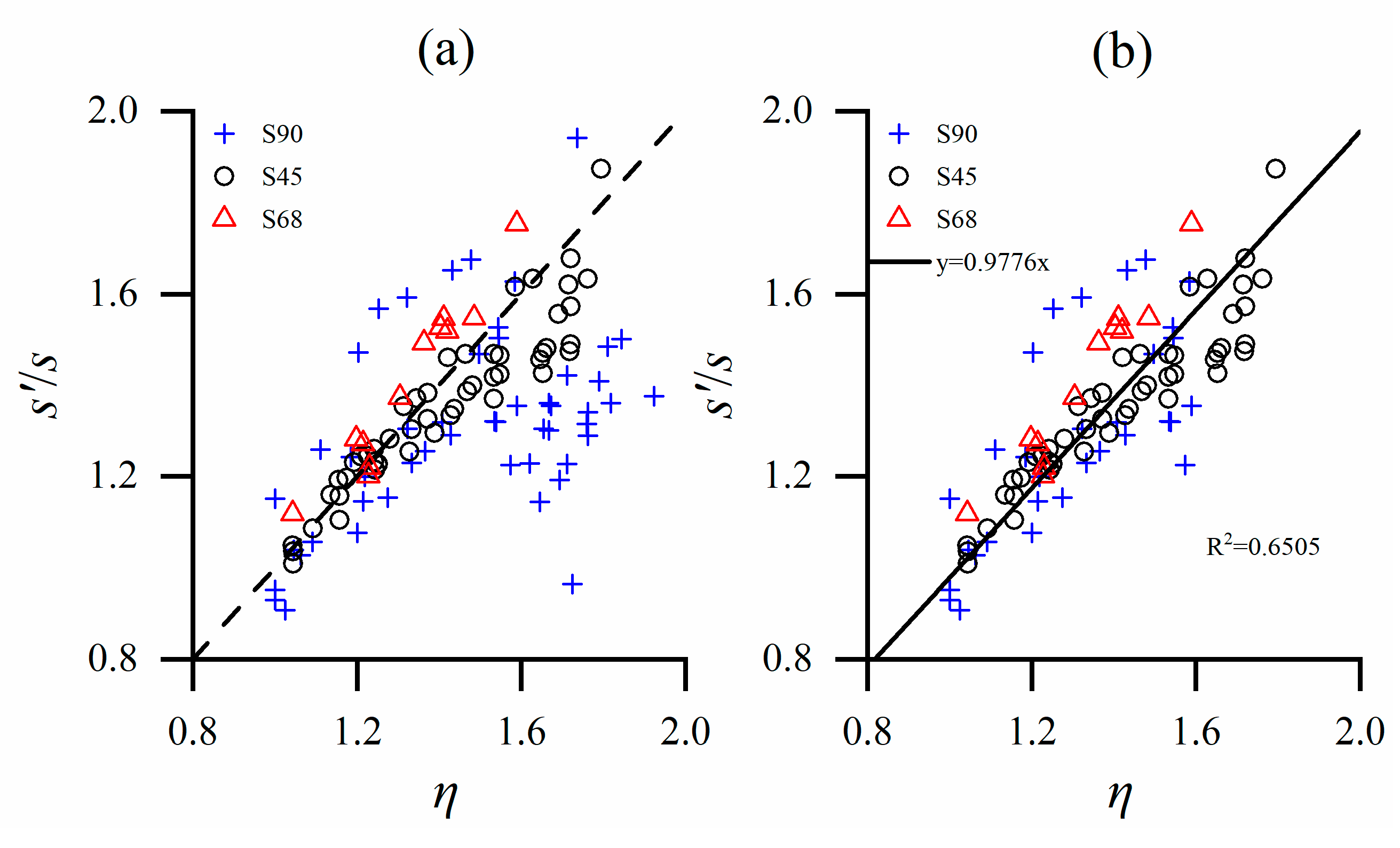
Based on the experimental data SFwm (112 experimental values of Type 1 from smooth boundary cases that are mentioned in Section 4.1, S90, S45, and S68 denote a smooth rectangular cross-section, trapezoidal cross-section with θ = 45°, and trapezoidal cross-section with θ = 68°, respectively), the value of S′/S can be calculated using Equations (11a) and (3a). Figure 2a shows the comparison between S′/S and η. The RMSE (root mean square error) for all three cases, S90, S45, and S68 are 0.21, 0.29, 0.1, and 0.1, respectively. Some data of two parameters differ considerably, especially for the cases of S90 with a width-depth ratio B/H > 8.5. However, for these cases, the values of SFw are relatively small (SFwm < 0.15) and a small deviation (|SFwc − SFwm|< 0.03) would cause large variations for S′/S. Conversely, the large difference between η and S′/S would not induce large deviation for SFw. Eliminating these data, Figure 2b shows the strong correlation (R2 = 0.65) between η and S′/S. Therefore, the value of S′/S can be roughly replaced by η.
4. New Methods and Comparisons
As η has been used to represent the value of S′/S, a new method based on the “equal local-region velocity” assumption has been established to determine the dividing lines and calculate boundary shear stress: (i) determine the value of k0 based on Equation (4); (ii) calculate k1 based on Equation (11a) (replacing S′/S by η) as Pb/Pw ≥ k0 − cosθ or calculate k2 based on Equation (11b) as Pb/Pw < k0 − cosθ (see details in Appendix A); (iii) calculate SFw based on Equation (3); and (iv) estimate the boundary shear stress in the wall-bed interaction zone as Equation (13), neglecting the effect of secondary currents:
in which L denotes the length of the zonal zone that is perpendicular to the boundary; g is gravitational acceleration.
The performance of different methods has been compared using two different cases: Smooth boundary cases and composite roughness cases.
4.1. Smooth Boundary Cases
The experimental data of smooth boundary cases have been used for comparisons between different methods. These experimental data (112 data for Type 1 and 28 for Type 2) includes: (i) smooth rectangular cases (S90) with 0.3 ≤ B/H ≤ 50: 69 experimental values (50 values of Type 1 and 19 values of Type 2) from the research work of [4,36,37,38,39,40,41,42,43]; (ii) smooth trapezoidal cases with θ = 45° (S45) with 0.3 ≤ B/H ≤ 15: 56 experimental values (50 values of Type 1 and 6 values of Type 2) from the research work of [2,37]; and (iii) smooth trapezoidal θ = 68° (S68) with 0.7 ≤ B/H ≤ 6.5: 15 experimental values (12 values of Type 1 and 3 values of Type 2) from the research work of [9].
There are two parameters that have been defined to represent the systematic deviation and accuracy of reproduction of measurements: Pε defined in Equation (14a) denotes the percentage of the calculated SFwc with an absolute error that is less than ε; En defined in Equation (14b) represents the systematic deviation of the calculated SFwc from the experimental value SFwm.
where “N” and “Nε” denotes total number of data and number of data with absolute error |SFwc − SFwm| ≤ ε; subscripts “c” and “m” denote the calculated values and measured values, respectively.
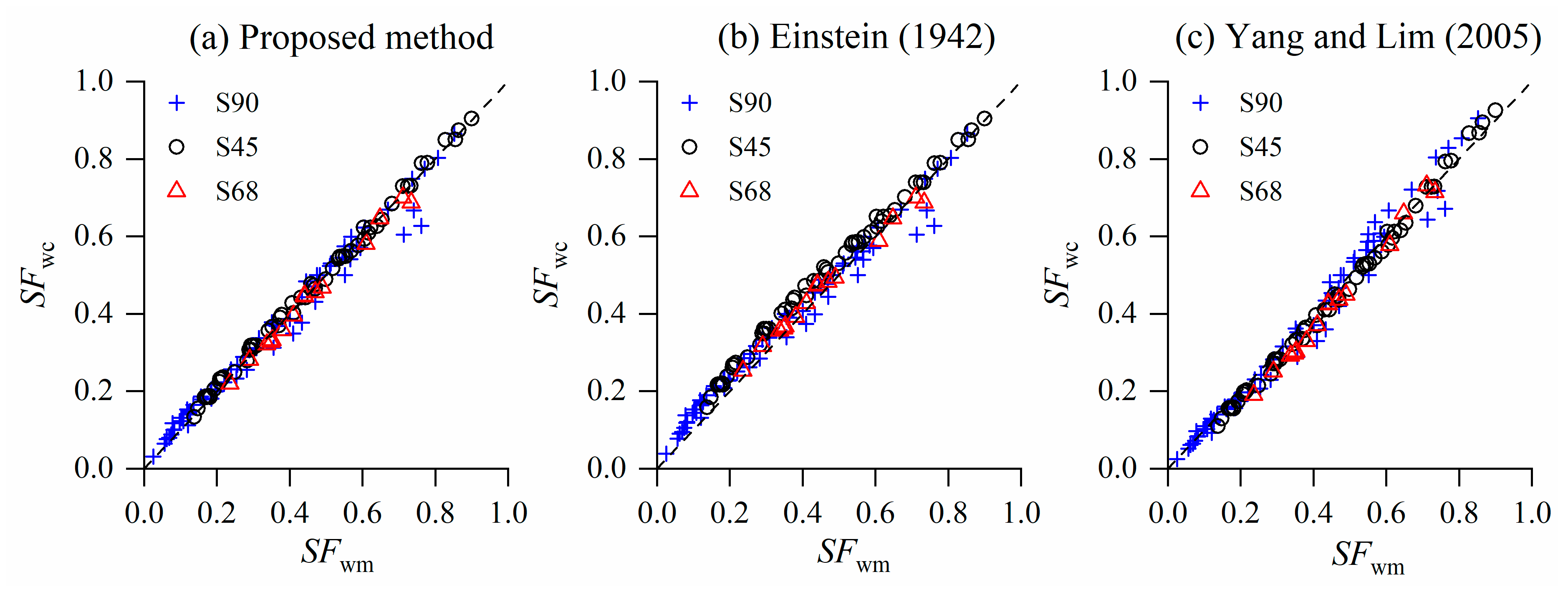
Among the analytical methods, Einstein’s method and YLM’s method are most simple ones. Figure 3 shows that the proposed method performs better compared to Einstein’s method and YLM’s method. For Type 2, both the proposed method and Einstein’s method are calculated based on Equation (11b). For Type 1, the performance indicators of the proposed method are P0.03 = 92.9%, P0.06 = 100%, and En = 4.7%, while those of Einstein’s method are P0.03 = 35.7%, P0.06 = 94.6%, and En = 16.4%. It indicates that the “equal local-region velocity” assumption actually improved the reproduction performance compared to Einstein’s “equal sub-region velocity” assumption. For all smooth boundary cases, the reproduction performance of the proposed method is P0.03 = 91.4%, P0.06 = 97.9%, and En = 3.5%, while that of YLM’s method is P0.03 = 71.6%, P0.06 = 94.3%, and En = −3.6%. Overall, the proposed method gives best performance among these three methods.
Several other analytical methods have also been used to calculate the boundary shear stress for both trapezoidal and rectangular cross-sections, for example, the methods of [26,27,28] (Figure 4). They also provide good reproduction of SFw; however, all of them include several empirical lumped correction factors. The empirical formulations of these correction factors that were obtained by the regression of experimental data are complex. Besides, similar to YLM’s method, the methods of [26,27] can only apply to smooth boundary cases. The method that was provided by [28], similar to Einstein’s method, can only calculate the average boundary shear stress of a wall-region or bed-region.
4.2. Composite Roughness Cases
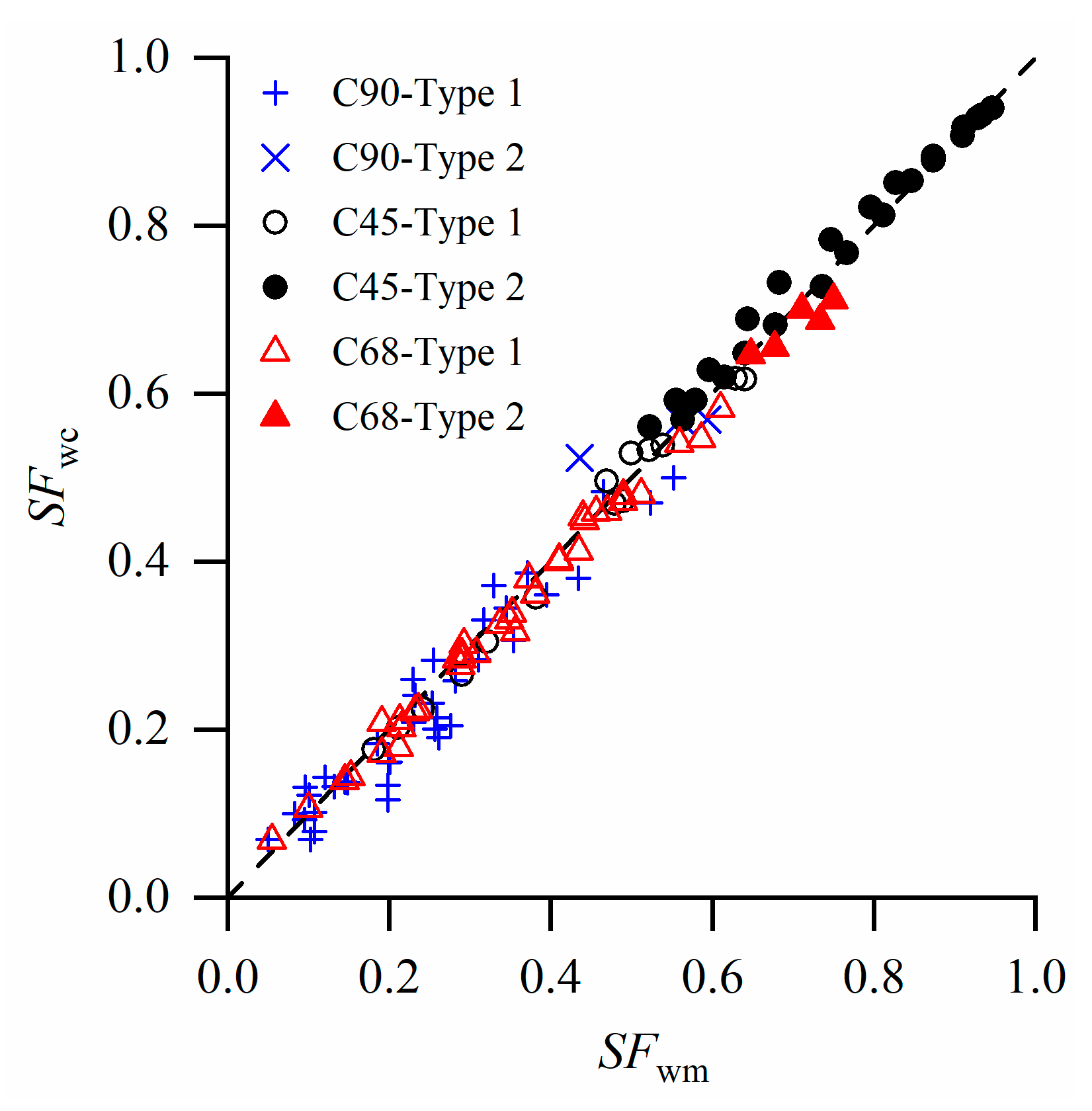
The composite roughness cases include two different categories, the first category is that both the bed and side-wall are hydraulically rough, but the roughness for the two are different; the second category is that the side-wall or bed is hydraulically smooth, while the other is hydraulically rough. The experimental data of composite roughness cases include: (i) composite rectangular cases (C90) with 1.5 ≤ B/H ≤ 15: 41 experimental values (38 values of Type 1 and 3 values of Type 2) from the research work of [39,40,44]; (ii) composite trapezoidal cases with θ = 45° (C45) with 0.7 ≤ B/H ≤ 9: 38 experimental values (14 values of Type 1 and 24 values of Type 2) from the research work of [45]; and (iii) composite trapezoidal θ = 68° (C68) with 0.85 ≤ B/H ≤ 10: 41 experimental values (36 values of Type 1 and 5 values of Type 2) from the research work of [9]. For the C90 and C68 cases, the values of roughness have been provided in the form of side-wall to bed roughness ksw/ksb. To calculate the resistance coefficient f, the reference roughness has been assumed: (a) Nikuradse’s equivalent roughness ks = 0.0015 mm is used for the smooth boundary of C90 cases; and (b) Nikuradse’s equivalent roughness of the plywood boundary is assumed to be ks = 0.05 mm. Figure 5 indicates that the proposed method also provides acceptable performance of SFw for composite roughness cases.
Few methods can be used to predict boundary shear stress for composite roughness cases. Among them are the Einstein’s method, methods of [9,28]. The empirical formulation that was established by [9] does not apply to C90 cases [28]. For C45 cases, the calculation accuracy based on the proposed method is P0.03 = 84.2% and P0.06 = 100%, which is close to that based on [28] with P0.03 = 89.5% and P0.06 = 100%. For Type 1 cross-sections of C45 cases, the proposed method improves the calculation accuracy compared to Einstein’s method. The calculation accuracy based on the proposed method is P0.03 = P0.06 = 100%, compared to P0.03 = 14.3% and P0.06 = 92.9% based on Einstein’s method. Experimental data of C90 and C68 cases have not been employed for comparison since the reference roughness has been assumed.
5. Discussion
5.1. The Effect of Secondary Currents and Empirical Treatments
The effect of secondary currents is to adjust the distribution of boundary shear stress. As the velocity distribution in Zonal(z) or Zonal(y) is 2D distribution, the average velocity VZonal increases with increasing length of the zonal zone. The gradient of velocity VZonal between adjacent zonals would induce secondary currents that transfer energy from high velocity zones (with large zonal length) to low velocity zones (with small zonal length) and then adjust the distribution of velocity and boundary shear stress. Due to the effect of secondary currents, the zero-shear stress dividing lines may not be straight lines as assumed in the new partition model.
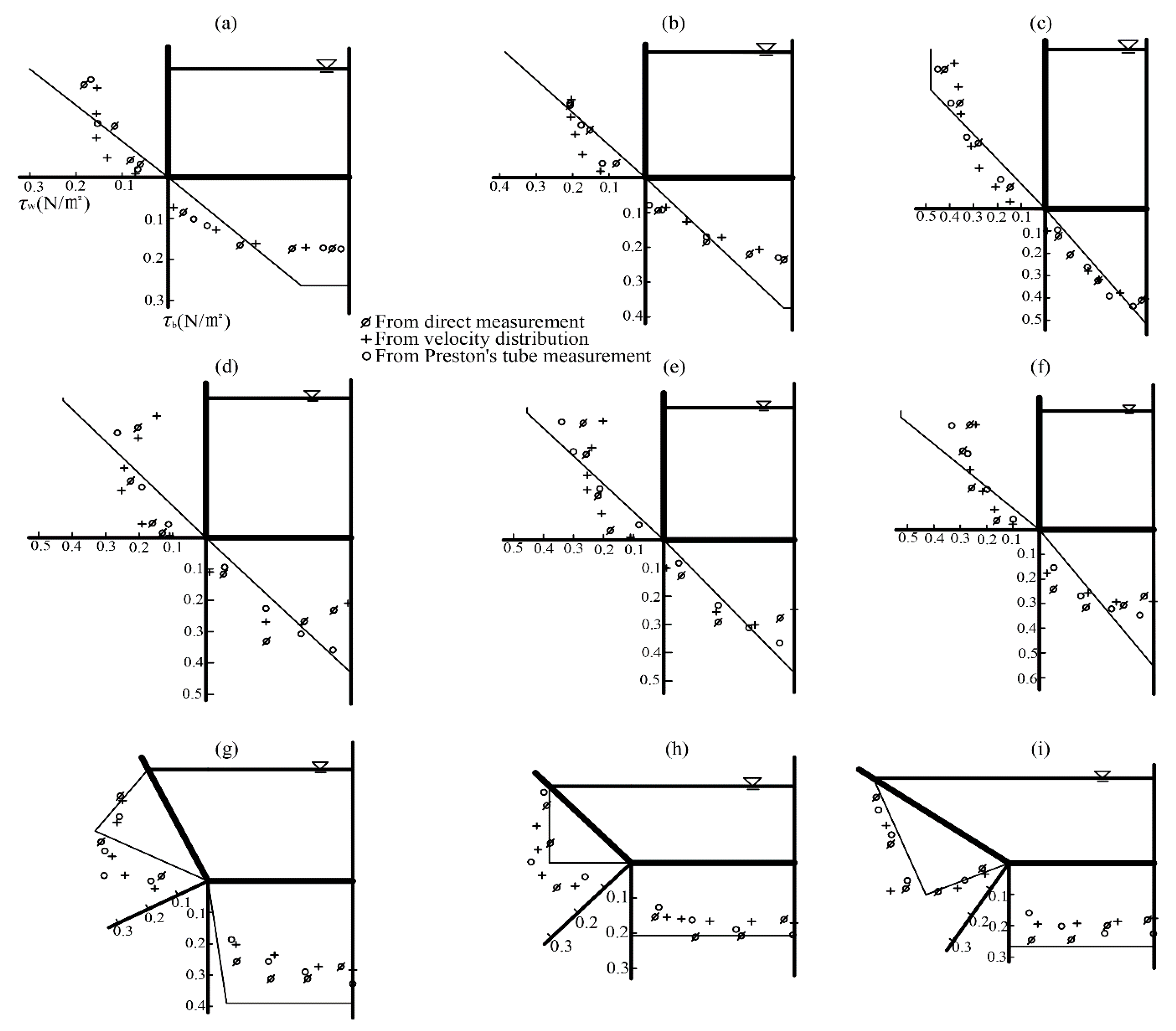
Ref. [37] measured the boundary shear stress distribution in rectangular/trapezoidal channels. Figure 6 shows the comparisons between the measured and calculated shear stress: (i) the calculated local shear stress is relatively larger compared to experimental results for a high velocity region (i.e., region with large zonal length Lzonal); (ii) the calculated local shear stress is relatively smaller compared to the experiment results for a low velocity region (i.e., region with small zonal length Lzonal); and (iii) the mean values of the calculated and experimental results are basically equal. These results show that the secondary currents adjust the distribution of velocity and energy in the separated region and transfer the downstream momentum from a high velocity region to a low velocity region.
For Type 1 and Type 2, different empirical treatments have been employed. For Type 1, the effect of secondary currents has been neglected and the influence of a center part of the bed-region is considered. For Type 2, the average velocities of a half wall-region and a half bed-region are assumed to be equal considering that the effect of the secondary currents in the wall-region on both the wall-region and bed-region cannot be neglected. These empirical treatments have been proven to be effective for smooth and composite roughness cases (see Section 4).
5.2. The Improvement of the Proposed Method
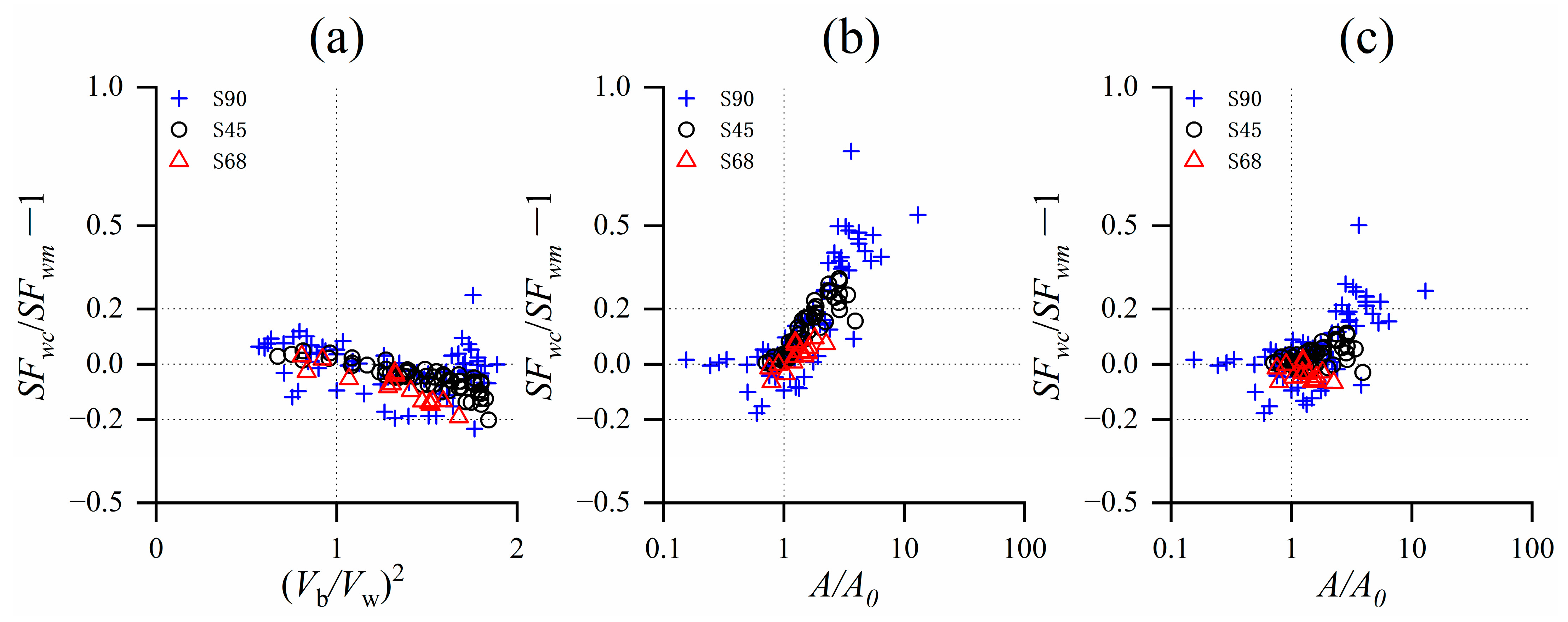
Figure 7 shows that the values of SFwc based on Einstein’s method are relatively larger than SFwm with a large aspect ratio. It may be caused by the fact that the equal sub-region velocity assumption neglects the non-uniform distribution of velocity in the bed-region for a Type 1 cross-section. Compared to Einstein’s method, the proposed method made some improvements. The relative error (SFwc/SFwm − 1) of several data of S90 with a large width-depth ratio (accordingly small value of SFw) based on the proposed method is larger than 0.2, however, the corresponding absolute error (SFwc − SFwm) is actually small, less than 0.02.
The results indicate that the “equal local-region velocity” assumption can be regarded as an improvement of Einstein’s equal velocity assumption [19]. There are two differences between Einstein’s assumption and the proposed method: (i) the proposed method provides two specific dividing lines that are determined by k1 and k2, while Einstein’s method did not; (ii) the proposed method assumes Vw = VbL for a Type 1 cross-section, while Einstein’s method neglects the non-uniform distribution of velocity in bed-region and assumes Vw = Vb.
Both YLM’s method and the proposed method define two “zero-shear stress” dividing lines by k1 and k2, and the distribution of boundary shear stress can be obtained based on Equation (13) for both methods as a dividing line has been specifically given [22]. YLM’s method introduced a “minimum relative distance of energy transportation” assumption to simplify the term for energy transfer, while the proposed method employed a new partition model. However, both of the methods neglect the effect of secondary currents.
For YLM’s method, the deviation of the calculated SFwc from SFwm is strongly related to the ratio between the average velocity of the bed-region and wall-region Vb/Vw: For a standardized cross-section with Vb = Vw, SFwc ≈ SFwm; for a Type 1 cross-section with Vb > Vw, SFwc < SFwm; and for a Type 2 cross-section with Vb < Vw, SFwc > SFwm (Figure 7). The most possible explanation is that YLM’s method neglects an important velocity condition that the velocities at two points that are divided by the “zero-shear stress” dividing line should be equal (i.e., umy = umz in Figure 1). Compared to YLM’s method, the proposed method does not show the systematic deviation although the relative error (SFwc/SFwm –1) of some cases with a small value of SFwc (less than 0.1) is larger than 0.2. As mentioned in Section 4, the proposed method gives better performance than YLM’s method for smooth cases.
Besides, YLM’s method used characteristic lengths that were represented by u∗ and ks to determine k1 and k2 for smooth and rough boundary cases, respectively. Since YLM’s method employed different parameters (u∗ and ks) to determine k1 and k2 for smooth and rough boundary cases, it does not apply to the situation that the turbulent flow patterns are different in the bed-region and wall-region. The proposed method, which employed the equal local-region velocity assumption to calculate k1 and k2, does not have this limitation.
6. Conclusions
Based on the experimental evidence of zero-shear stress dividing line, a new partition model of a cross-section has been introduced. The kinetic energy equation has been employed to analyze the flow characteristics in the bed-wall interaction zone and an “equal local-region velocity” assumption has been proposed. Based on this assumption, the zero-shear stress dividing line can be determined and then the distribution of boundary shear stress can be calculated.
The proposed method has established a new partition model of a cross-section with the assumption of the existence of the zero-shear stress dividing lines. There are two types of cross-section that are introduced referring to a standardized cross-section. In this model, the interaction or energy transfer between the sub-regions can be neglected since these sub-regions are cut by zero-shear stress dividing lines.
The proposed method can be used to estimate the average shear stress of a bed or wall region. The comparisons show that the proposed method provides better reproduction performance for all smooth boundary cases compared to other methods and can also be applied to composite roughness cases. However, more composite roughness cases are needed for further justification of this method. The proposed method can also provide a preliminary distribution of shear stress neglecting the effect of the secondary currents.
Author Contributions
Conceptualization, Methodology, funding acquisition, writing—original draft preparation, Y.L.; writing—review and editing, S.Z.; validation and calculation, F.Y., W.G., C.Y. and R.Y. All authors have read and agreed to the published version of the manuscript.
Funding
National Nature Science Foundation of China (No. 51409132).
Institutional Review Board Statement
Not applicable.
Informed Consent Statement
Not applicable.
Data Availability Statement
The data of the ratio of boundary shear force of wall to total shear force (SFw), and corresponding geometry parameters of the cross-sections of S90, S45, S68, C90, C45, and C68 that are mentioned in Section 4 are available from the corresponding author upon reasonable request. All the data that are mentioned are laboratory data.
Acknowledgments
The authors gratefully acknowledge Professor Weiming Wu, Clarkson University, who provided valuable advice on this paper. The authors also would like to acknowledge the financial support from the National Nature Science Foundation of China (No. 51409132).
Conflicts of Interest
The authors declare no conflict of interest.
Appendix A
Appendix A.1. Calculation of Resistance Coefficient f
For some smooth boundary cases, the information about the boundary roughness and water depth are not included in some experimental data. Blasius formula [46], which has the simplest form (see A1) and is valid for the range of Reynold’s numbers Re: 4000 < Re < 80,000, has been employed to calculate the resistance coefficient.
For composite roughness cases (i.e., C90, C45, and C68 cases), a unified formula covering the hydraulically smooth and rough turbulent flows has been used for the calculation of friction factors [47,48]:
in which Equations (A3) and (A4) are used to calculate χs; Re∗ denotes the roughness Reynolds number Re∗ = u∗ks/ν, in which ν represents the kinetic viscosity; for smooth boundary cases with Re∗ < 1, Bs = 2.5lnRe∗ + 5.5.
Appendix A.2. Calculation of k1 and k2
For smooth boundary cases, Equation (A1) has been used to calculate f. In Equation (11a), the hydraulic radius of two local regions “EDF” and “EGF” are k1H/2 and H/2, respectively. Based on Equation (A1) and Darcy–Weisbach formula, we can obtain:
Based on Equations (11a), (12) and (A1), k1 can be calculated as:
in which k0 = 1 for smooth boundary cases.
Referring to Equation (A5), the term in the left of Equation (11b) should be:
Comparing Equations (11b) and (A6), gives:
Then k2 can be obtained by:
For rough boundary cases, the values of k1 and k2 can be obtained based on tentative calculation of Equations (11a) and (11b).
References
- Rajaratnam, N.; Muralidhar, D. Boundary shear stress distribution in rectangular open channels. Houille Blanche 1969, 1, 603–610. [Google Scholar] [CrossRef]
- Yuen, K.W.H. A Study of Boundary Shear Stress, Flow Resistance and Momentum Transfer in Open Channels with Simple and Compound Trapezoidal Cross Sections. Ph.D. Thesis, University of Birmingham, Birmingham, UK, 1989. [Google Scholar]
- Khodashenas, S.R.; Paquier, A. A geometrical method for computing the distribution of boundary shear stress across irregular straight open channels. J. Hydraul. Res. 1999, 37, 381–388. [Google Scholar] [CrossRef]
- Knight, D.W.; Demetriou, J.D.; Hamed, M.E. Boundary shear in smooth rectangular channels. J. Hydraul. Eng. 1984, 110, 405–422. [Google Scholar] [CrossRef]
- Cacqueray, N.D.; Hargreaves, D.M.; Morvan, H.P. A computational study of shear stress in smooth rectangular channels. J. Hydraul. Res. 2009, 47, 50–57. [Google Scholar] [CrossRef]
- Yang, S.Q.; Lim, S.Y. Mechanism of energy transportation and turbulent flow in a 3D channel. J. Hydraul. Eng. 1997, 123, 684–692. [Google Scholar] [CrossRef]
- Ansari, K.; Morvan, H.P.; Hargreaves, D.M. Numerical investigation into secondary currents and wall shear in trapezoidal channels. J. Hydraul. Eng. 2011, 137, 432–440. [Google Scholar] [CrossRef]
- Khodashenas, S.R.; El kadi Abderrezzak, K.; Paquier, A. Boundary shear stress in open channel flow: A comparison among six methods. J. Hydraul. Res. 2008, 46, 598–609. [Google Scholar] [CrossRef]
- Flintham, T.P.; Carling, P.A. Prediction of mean bed and wall boundary shear in uniform and compositely rough channels. In International Conference on River Regime; Hydraulics Research Limited: Wallingford, UK, 1988; pp. 267–287. [Google Scholar]
- Khozani, Z.S.; Bonakdari, H.; Zaji, A.H. Using two soft computing methods to predict wall and bed shear stress in smooth rectangular channels. Appl. Water Sci. 2017, 7, 3973–3983. [Google Scholar] [CrossRef]
- Vazquez, P.M.; Sharifi, S. Modelling boundary shear stress distribution in open channels using a face recognition technique. J. Hydroinform. 2017, 19, 157–172. [Google Scholar] [CrossRef]
- Wormleaton, P.R.; Merrett, D.J. An improved method of calculation for steady uniform flow in prismatic main channel/flood plain sections. J. Hydraul. Res. 1990, 28, 157–174. [Google Scholar] [CrossRef]
- Prinos, P.; Townsend, R.D. Comparison of methods for predicting discharge in compound open channels. Adv. Water Resour. 1984, 7, 180–187. [Google Scholar] [CrossRef]
- Moreta, P.J.; Martin-Vide, J.P. Apparent friction coefficient in straight compound channels. J. Hydraul. Res. 2010, 48, 169–177. [Google Scholar] [CrossRef]
- Chen, Z.; Chen, Q.; Jiang, L. Determination of apparent shear stress and its application in compound channels. Procedia Eng. 2016, 154, 459–466. [Google Scholar] [CrossRef]
- Leighly, J.B. Toward a theory of the morphologic significance of turbulence in the flow of water in streams. Prog. Phys. Geogr. 1932, 6, 1–22. [Google Scholar]
- Nezu, I.; Nakagawa, H.E.D. Turbulence in Open-Channel Fows; Balkema: Rotterdam, The Netherlands, 1993. [Google Scholar]
- Keulegan, G.H. Laws of turbulent flow in open channels. J. Res. Natl. Bur. Stand. 1938, 21, 708–741. [Google Scholar] [CrossRef]
- Einstein, H.A. Formulas for the transportation of bed load. Trans. ASCE 1942, 107, 561–597. [Google Scholar] [CrossRef]
- Chien, N.; Wang, Z. Mechanics of Sediment Transport; Science Press: Beijing, China, 1986. (In Chinese) [Google Scholar]
- Yang, S.Q.; Lim, S.Y. Boundary shear stresses distributions in smooth rectangular open channel flows. Proc. Inst. Civ. Eng.-Water Marit. Energy 1998, 130, 163–173. [Google Scholar]
- Yang, S.Q.; Lim, S.Y. Boundary shear stress distributions in trapezoidal channels. J. Hydraul. Res. 2005, 43, 98–102. [Google Scholar] [CrossRef]
- Yang, S.Q.; Yu, J.X.; Wang, Y.Z. Estimation of diffusion coefficients, lateral shear stress, and velocity in open channels with complex geometry. Water Resour. Res. 2004, 40, W05202. [Google Scholar] [CrossRef]
- Shiono, K.; Knight, D.W. Turbulent open-channel flows with variable depth across the channel. J. Fluid Mech. 1991, 222, 617–646. [Google Scholar] [CrossRef]
- Guo, J.; Julien, P.Y. Shear stress in smooth rectangular open-channel flows. J. Hydraul. Eng. 2005, 131, 30–37. [Google Scholar] [CrossRef]
- Kabiri-Samani, A.; Farshi, F.; Chamani, M.R. Boundary Shear Stress in Smooth Trapezoidal Open Channel Flows. J. Hydraul. Eng. 2013, 139, 205–212. [Google Scholar] [CrossRef]
- Javid, S.; Mohammadi, M. Boundary shear stress in a trapezoidal channel. Int. J. Eng. 2012, 25, 323–332. [Google Scholar] [CrossRef]
- Luo, Y.; Zhu, S.; Cao, B.; Jiang, C.J. A “Standard Cross-section” Method for the calculation of Riverbed and Bank shear stress. Appl. Math. Mech. 2021, 42, 915–923. (In Chinese) [Google Scholar]
- Han, Y.; Yang, S.Q.; Sivakumar, M.; Qiu, L.C.; Chen, J. Flow Partitioning in Rectangular Open Channel Flow. Math. Probl. Eng. 2018, 2018, 11. [Google Scholar] [CrossRef]
- Yang, S.Q.; Han, Y.; Lin, P.; Jiang, C.; Walker, R. Experimental study on the validity of flow region division. J. Hydro-Environ. Res. 2014, 8, 421–427. [Google Scholar] [CrossRef]
- Han, Y.; Yang, S.Q.; Dharmasiri, N.; Sivakumar, M. Experimental study of smooth channel flow division based on velocity distribution. J. Hydraul. Eng. 2015, 141, 06014025. [Google Scholar] [CrossRef]
- Johnson, J.W. The importance of considering sidewall friction in bed-load investigations. Civil Eng. 1942, 12, 329–332. [Google Scholar]
- Vanoni, V.A.; Brooks, N.H. Laboratory Studies of the Roughness and Suspended Load of Alluvial Streams; Sedimentation Laboratory Report No. E68; California Institute of Technology: Pasadena, CA, USA, 1957. [Google Scholar]
- Nezu, I.; Nakagawa, H.E.D.; Tominaga, H. Secondary currents in a straight channel flow and the relation to its aspect ratio. Turbul. Shear. Flows 1985, 4, 246–260. [Google Scholar]
- State Key Laboratory of Hydraulics and Mountain River Engineering (SKLHMRE). Hydraulics; Higher Education Press: Beijing, China, 2015; p. 131. (In Chinese) [Google Scholar]
- Cruff, R.W. Cross-Channel Transfer of Linear Momentum in Smooth Rectangular Channels; Water-Supply Paper 1592-B, United States Geological Survey: Reston, VA, USA, 1965. [Google Scholar]
- Ghosh, S.N.; Roy, N. Boundary shear distribution in open channel flow. J. Hydraul. Div. 1970, 96, 967–994. [Google Scholar] [CrossRef]
- Kartha, V.C.; Leutheusser, H.J. Distribution of tractive force in open channels. J. Hydraul. Div. 1970, 96, 1469–1483. [Google Scholar] [CrossRef]
- Knight, D.W.; Macdonald, J.A. Hydraulic resistance of artificial strip roughness. J. Hydraul. Div. 1979, 105, 675–690. [Google Scholar] [CrossRef]
- Knight, D.W.; Macdonald, J.A. Open channel flow with varying bed roughness. J. Hydraul. Div. 1979, 105, 1167–1183. [Google Scholar] [CrossRef]
- Myers, W.R.C. Flow resistance in wide rectangular channels. J. Hydraul. Div. 1982, 108, 471–482. [Google Scholar] [CrossRef]
- Noutsopoulos, G.C.; Hadjipanos, P. Discussion: Boundary Shear in Smooth and Rough Channels. J. Hydraul. Div. 1982, 108, 809–812. [Google Scholar] [CrossRef]
- Seckin, G.; Seckin, N.; Yurtal, R. Boundary shear stress analysis in smooth rectangular channels. Can. J. Civ. Eng. 2006, 33, 336–342. [Google Scholar] [CrossRef]
- Knight, D.W. Boundary shear in smooth and rough channels. J. Hydraul. Div. 1981, 107, 839–851. [Google Scholar] [CrossRef]
- Alhamid, A.I. Boundary Shear Stress and Velocity Distribution in Differentially Roughened Trapezoidal Open Channels. Ph.D. Thesis, University of Birmingham, Birmingham, UK, 1991. [Google Scholar]
- Blasius, H. Das Ähnlichkeitsgesetz bei Reibungsvorgängen in Flüssigkeiten; Forschungs-Arbeit des Ingenieur-Wesens 131; Springer: Berlin/Heidelberg, Germany, 1913. (In German) [Google Scholar]
- Einstein, H.A. The Bed-Load Function for Sediment Transportation in Open Channel Flows; Technical Bulletin No. 1026, U.S. Department of Agriculture, Soil Conservation Service: Washington, DC, USA, 1950. [Google Scholar]
- Da Silva, A.M.F.; Bolisetti, T. A method for the formulation of Reynolds number functions. Can. J. Civil Eng. 2000, 27, 829–833. [Google Scholar] [CrossRef]
Figure 1.
Partition model of a cross-section: (a) standardized section, (b) Type 1 section, and (c) Type 2 section.
Figure 1.
Partition model of a cross-section: (a) standardized section, (b) Type 1 section, and (c) Type 2 section.

Figure 2.
Relationship between S’/S calculated based on SFwm and η for smooth boundary cases: (a) comparisons between them, and (b) linear regression neglecting some data.
Figure 2.
Relationship between S’/S calculated based on SFwm and η for smooth boundary cases: (a) comparisons between them, and (b) linear regression neglecting some data.


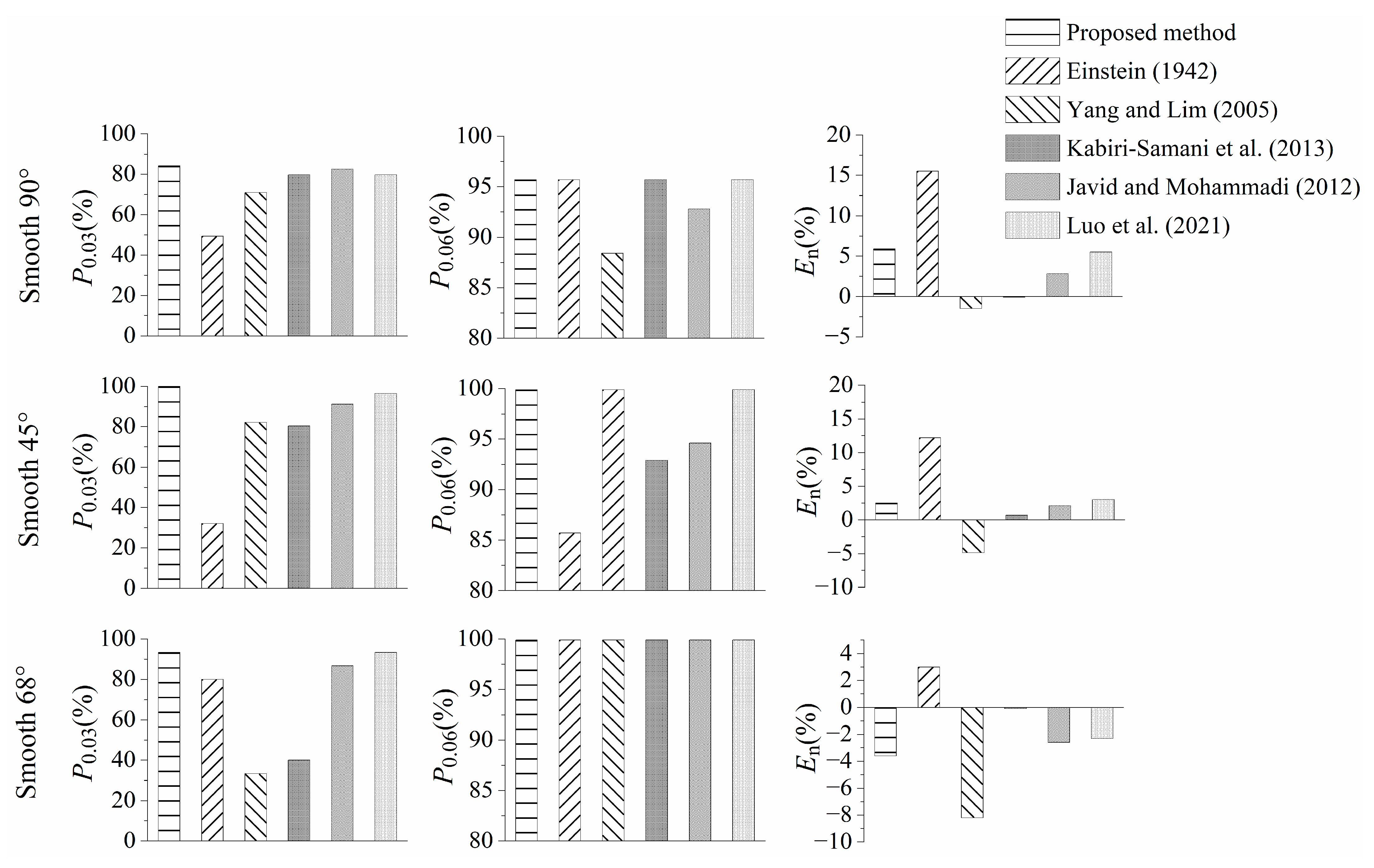
Figure 4.
Performance of different methods for smooth boundary cases (Einstein 1942 [19], Yang and Lim 2005 [22], Kabiri-Samani et al. 2013 [26], Javid and Mohammadi 2012 [27], Luo et al. 2021 [28]).

Figure 5.
Comparisons of the measured data and the calculated results for composite roughness cases.
Figure 5.
Comparisons of the measured data and the calculated results for composite roughness cases.

Figure 6.
Comparisons of the calculated (denoted by fine lines) and measured boundary shear stress distribution: (a) Smooth, θ = 90° and Pb/Pw = 1.56; (b) Smooth, θ = 90° and Pb/Pw = 1.09; (c) Smooth, θ = 90° and Pb/Pw = 0.6; (d) Rough (ks = 1.04 mm), θ = 90° and Pb/Pw = 0.98; (e) Rough (ks = 1.85 mm), θ = 90° and Pb/Pw = 0.92; (f) Rough (ks = 3.17 mm), θ = 90° and Pb/Pw = 0.9, (g) Rough (ks = 3.17 mm), θ = 63.4° and Pb/Pw = 1.09; (h) Rough (ks = 3.17 mm), θ = 45° and Pb/Pw = 1.41 (i) Rough (ks = 3.17 mm), θ = 33.7° and Pb/Pw = 0.89.

Figure 7.
Limitation of different methods: (a) YLM’s method, (b) Einstein’s method, and (c) the proposed method.
Figure 7.
Limitation of different methods: (a) YLM’s method, (b) Einstein’s method, and (c) the proposed method.

Publisher’s Note: MDPI stays neutral with regard to jurisdictional claims in published maps and institutional affiliations. |
© 2022 by the authors. Licensee MDPI, Basel, Switzerland. This article is an open access article distributed under the terms and conditions of the Creative Commons Attribution (CC BY) license (https://creativecommons.org/licenses/by/4.0/).
Share and Cite
MDPI and ACS Style
Luo, Y.; Zhu, S.; Yang, F.; Gao, W.; Yan, C.; Yan, R. Estimation of Boundary Shear Stress Distribution in a Trapezoidal Cross-Section Channel with Composite Roughness. Water 2022, 14, 2530. https://doi.org/10.3390/w14162530
AMA Style
Luo Y, Zhu S, Yang F, Gao W, Yan C, Yan R. Estimation of Boundary Shear Stress Distribution in a Trapezoidal Cross-Section Channel with Composite Roughness. Water. 2022; 14(16):2530. https://doi.org/10.3390/w14162530
Chicago/Turabian StyleLuo, You, Senlin Zhu, Fan Yang, Wenxiang Gao, Caiming Yan, and Rencong Yan. 2022. "Estimation of Boundary Shear Stress Distribution in a Trapezoidal Cross-Section Channel with Composite Roughness" Water 14, no. 16: 2530. https://doi.org/10.3390/w14162530
Note that from the first issue of 2016, this journal uses article numbers instead of page numbers. See further details here.