
The Effect of Urban Agriculture on Water Security: A Spatial Approach


1
Graduate School of Environmental Engineering, University of Kitakyushu, Kitakyushu 808-0135, Japan
2
Faculty of Environmental Engineering, University of Kitakyushu, Kitakyushu 808-0135, Japan
*
Author to whom correspondence should be addressed.
Water 2022, 14(16), 2529; https://doi.org/10.3390/w14162529
Submission received: 22 June 2022
/
Revised: 13 August 2022
/
Accepted: 15 August 2022
/
Published: 17 August 2022
(This article belongs to the Special Issue Water Resources Management and Social Issues)
Abstract
:This study aimed to examine the influence of agricultural development under urbanization on agriculture water supply internalization. Water supply internalization is the process of measuring water security to estimate the degree of water supply sustainably by region inside. According to water users, Water supply internalization could be divided into Agriculture and urban water supply internalization. Agriculture and urban water supply internalization are calculated in this study. This study employed a spatial model to analyze agricultural water supply internalization and its influencing factors. The results showed that the agriculture development associated with agricultural population and crop typology impacts agricultural water supply internalization. Urban water supply internalization increases lead to an increase in agricultural water supply internalization. The agricultural population’s spatial agglomerations lead to increased agricultural water supply internalization. Agricultural population’s spatial agglomerations mean neighborhood city agriculture population share similar trend. Agricultural and urban water supply internalization have spatial autoconnection. The study area consisted of 30 cities in four provinces in North China: Beijing, Tianjin, Hebei, and Shandong.
1. Introduction
The development of society causes water scarcity problems worldwide. Rapid urbanization brings anthropogenic effects on agriculture and the water environment. Under climate change, urban areas will produce a surface water deficit of 1386–6764 million m3 per year worldwide [1]. Agricultural water accounts for the highest proportion among water consumption amounts. Its withdrawals will increase by 13% and reach 2975 km3 in 2050 versus 2000 [2]. Both urban and agricultural water face the limitation of water resources. When they share the same water resources, urban water has competition with agricultural water [3].
The development of agriculture brings huge changes in agricultural social aspects, such as changes in patterns of land use and population [4]. The development of agriculture alters the water supply. Auci (2021) found climate, irrigation propensity indicator, and yields affect irrigation [5]. Zhao et al. (2014) studied the influencing factors of food production to water [6]. The influencing factors consist of population, Gross Domestic Product (GDP), urbanization, and diet structure. Agricultural water use is related to urban development in two ways. Firstly, urban development promotes agricultural development, improves technology, and attracts agricultural population and related resources [7]. Secondly, urban water use is related to agricultural water use. Urbanization leads to an increase in water withdrawal.
China faces severe water scarcity due to rapid economic development and urbanization, especially with a large and growing population [8]. According to the Chinese Statistics Yearbook 2018, under the limitation of water resources, the contradiction of water allocation for urban and agricultural activities is prominent [9]. Now, China’s agriculture depends significantly on irrigation [10]. China’s water resources have an unbalanced distribution problem [11]. It is essential to maintain the water supply security in water-scarce areas.
Water security is defined to maintain the sustainable water supply even if external water sources are limited. Water security focuses on the quantity and availability of water. Its main issue is demand-driven scarcity, which is the ratio to measure how much water is withdrawn from rivers and aquifers in an area [12,13]. We use water supply internalization to measure water security. It extends supplies from internal water sources in a geographical area and decreases reliance on water drawn from outside sources [14]. We consider the boundary of the “internal area” as the city-level boundary in Northern China. Water supply in an area consists of urban and agricultural water supply. Agricultural water supply internalization (AWS) is the security of agricultural water. Urban water supply internalization (UWS) is the security of urban water. Water security is affected by spatial agglomeration. Spatial agglomeration refers to the geographical pattern where the same feature appears in proximity to each other [15]. The spatial agglomeration of agricultural and urban activities affects the environment. Zhong et al. (2020) found that the economic and social development of the surrounding cities impacted local agricultural activities [16]. Urbanization spatially reduces the ecological footprint of agricultural water [17]. At the same time, agriculture values keep increasing. Agriculture water use efficiency increases under spatial agglomeration. We wanted to study the spatial agglomeration effect on the water environment through water security indicators. Mu et al. (2021) began to use water indicators and spatial analyses together. They used one indicator and conducted a spatial autocorrelation analysis [18]. We advance this approach and analyze spatial autocorrelation and spatial agglomeration of AWS and UWS using two indicators. Following that, we applied multiple methods of spatial analysis.
We studied the effects of agriculture development on AWS under urbanization. We used spatial models and address two research questions: first, how does agricultural development directly affect AWS? Second, how does urbanization affect AWS by changing urban water supply?
2. Literature Review
According to the 2008 World Development Report, agricultural development entails both gains in terms of aggregate income and total labor force. Development is accompanied by technological improvement progress [19]. Improving technology is essential for balancing the water environment and the economy. Li (2020) used the Mann–Kendall method and GIS to study the agriculture scale and planting structure effect on water. By an adjustment of the planting structure, the agricultural sector could increase the scale of irrigated by as much as 25.8% [20]. Galioto et al. (2020) used a comparative cost–benefit analysis based on the value of information approach. They found that the implementation of an alternative technology generates a 0–20% increase in gross yield margin and a 10–30% water saving compared existing irrigation practices [21]. Song et al. (2018) used undesirable output-based Malmquist–Luenberger productivity index and found that technical improvements contributed to water resource efficiency [22].
Indicator methods are used for measuring the characteristics of the water environment. The agricultural water stress index can reveal agricultural water shortages. It could provide suggestions for agricultural development and water use in the water-scarce area, such as the north grain-producing areas in China [23].
Industrial structure upgrading and population expansion could significantly affect water use. Different sectors have different scales of water use. Agriculture consumes the most water. Water resources can be an economic constraint [24].
An increase in urban water demand leads to water competition between urban water and agricultural water, especially when they share the similar water supply source, the local water resource. The agricultural sector is high in water consumption but low in economic efficiency. Human society needs to coordinate water use among different sectors [25]. Antoci (2017) conducted a theoretical analysis and found that competing water-use sectors have different relationships in various economic situations [26].
3. Method
3.1. Study Area
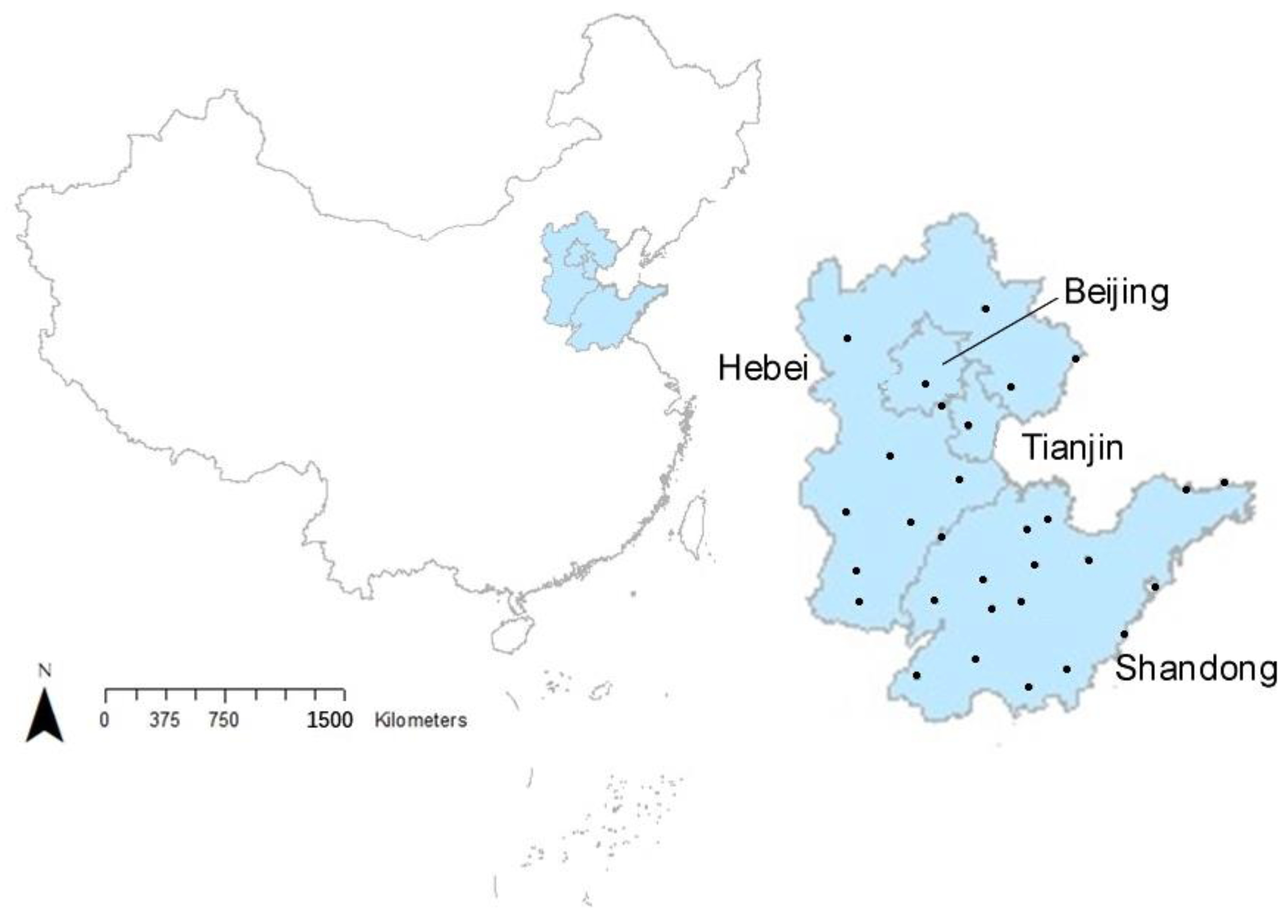
We studied the North China Plain, which is a water-scarce area. We focused on four East coast provinces: Beijing, Tianjin, Hebei, and Shandong (Figure 1). According to Falkenmark (1989, 1992), water scarcity areas are defined by per capita water amounts below 500 m3 annum [27,28]. The annual water per person in the four provinces is less than 500 m3 (China Statistic Year Book and China Water Bulletin). These cities have faced conflicts between agricultural and urban activities. These four provinces are the main producing areas for water-consuming crops. Wheat production in Henan, Shandong, and Hebei provinces accounts for more than 50% of the total national production [29]. The growth cycle of winter wheat in North China is in winter and spring with little rainfall, and wheat production consumes a large amount of blue water [30]. Besides, these provinces have developed urban areas. Beijing and Tianjin were designated province-level cities. Shandong and Hebei experienced rapid urbanization. The urbanization of Shandong increased from 48.32% in 2009 to 60.58% in 2017. Hebei’s grew from 43.74% in 2009 to 55.01% in 2017. We studied 30 cities in the four provinces.
3.2. Water Supply Internalization Indicator
Under the sustainable development goals indicator framework, water supply internalization is important in measuring water supply pressure and the sustainability of the water environment. Water supply sectors can be divided into agricultural and urban water sectors. The agricultural water sector consumes the most water. Different regions have different levels of agricultural water-carrying capacity [31]. In this study, water supply internalization is the ratio of water supply to water resource amount, as shown in Equations (1) and (2). Agricultural water (AW) is the amount of water supplied to the agricultural industry within a city boundary. Urban water (UW) is the amount of urban and industrial water supply among the total water supply in the boundary. The water resource (WR) is the amount of natural water within the city boundary; it consists of freshwater lakes, rivers, and aquifers [32]. The following equations were used to calculate AWS and UWS. A smaller value in these indicators shows a decreased impact on the local water environment.
Table 1 describes basic statistics of the water supply internalization indicators and their elements. A smaller value of AWS means less impact to the local water environment. For our spatial autocorrelation models, AWS becomes the dependent variable and UWS becomes one of the independent variables.
3.3. Variables and Data
Table 2 summarizes the independent variables used for this study other than UWS. It also includes basic statistics. Independent variables included agricultural activities, climate factors, and others.
As for agricultural activities, we used affluence, agricultural population, and technology to measure agricultural activities. Affluence is the agricultural GDP. As for the technology, we used two aspects to measure: agricultural asset technology and crop typology. Agricultural asset technology refers to the total power of agricultural machines. Machine power has been used in many agricultural studies, such as [33]. We used crop typology to reflect the different crop cultivation areas. Crop typology is an essential part of agricultural social change. Auci and Vignani (2021) studied crop typology and irrigation water [5]. Traditional plant planting areas consist of grains and oilseeds. Vegetable planting areas were considered as an alternative crop type. Agricultural development could improve the agriculture arrangement [34].
As for climate factors, we used temperature and precipitation to represent the climate. Auci and Vignani (2021) studied the climatic factors that affected agricultural water. They studied two variables, temperature and precipitation, which separately represent the yearly annual temperature and the yearly amount of precipitation.
The water accessibility variable indicates the convenience of water acquisition, including outside resources [5]. We used four levels to represent the different locations. Level 1 indicates that the city is located in the Yellow River basin. Level 2 indicates that the city is in the Yellow River water transfer project area. Only seven cities are not located in the Yellow River basin or Yellow River water transfer project area. In these seven cities, three important cities have plans for south-to-north water transfer projects. These three cities were regarded as Level 3. Others are regarded as Level 4. A larger level indicates more difficulty in accessing large water resources. We used data of 30 cities from 2001 to 2016. Social factor data are from the local statistical yearbook; the local statistical yearbook includes the Beijing statistical yearbook, Tianjin Statistical yearbook, Hebei statistical yearbook, and Shandong statistical yearbook. Missing data were filled using local averages. Population data were obtained from the local statistical yearbook. Affluence from local statistical data. Technology from local statistical yearbooks. Plant area of Beijing Tianjin and Shandong were taken from local statistical yearbooks. The plant area of Hebei was obtained from the Hebei Rural Statistical Yearbook. The temperature data were obtained from the China Meteorological Administration. Local water resource, precipitation, and agricultural water supply amounts were compiled from the Beijing Water Resources Bulletin, Tianjin Water Resources Bulletin, Hebei Water Resources Bulletin, and Shandong Water Resources Bulletin. Hebei agricultural water amount was taken from the Hebei rural statistics yearbook.
3.4. Spatial Analysis Model
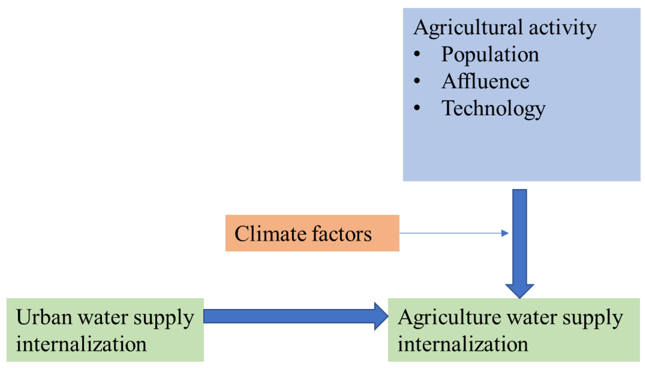
We assumed that agricultural activities and UWS affect AWS, and they are non-linear relationships. This model is illustrated in Figure 2. Agricultural population, affluence, and technology affect AWS. Based on the spatial econometric model, we consider the effects of agricultural production factors [35].
There are two steps to test the spatial agglomeration effect. The first step is to examine Global Moran’s I of the global spatial autocorrelation of agricultural and UWS. We measured AWS and UWS using Global Moran’s I from 2001 to 2016. It is used to identify the overall spatial autocorrelation for quantifying the degree of clustering or dispersion [36,37]. In this step, we examine the spatial dependency of these internalization indexes. The second step was to measure the spatially influential factors on water supply internalization using spatial models.
The Global Moran’s I, , is calculated across cities (j, j = 1–30). represents the spatial weight. We used the adjacency matrix as spatial weight; if the two cities are spatially adjacent, the value is 1; otherwise, it is 0. X is the AWS or UWS, and represents the average of those values. The Global Moran’s I is between −1 and 1. When I < 0, it indicates that the water supply internalization is negatively correlated across the adjacent cities; when I > 0, it indicates a positive correlation, and when I = 0, it indicates that there is no spatial correlation. Stata was used for calculating Global Moran’s I. Spatial empirical research is still developing [35,38,39]. Previous researchers introduced and developed spatial matrices. As for spatial panel analysis, Lee (2002) and Elhorst (2017) increased accuracy [38,40]. We use three different spatial models to measure the spatial influencing factors of water supply internalization. A Spatial Auto Regressive model (SAR) is shown in Equation (4). A Spatial-Error model (SEM) is shown in Equation (5). A spatial Durbin model (SDM) is shown in Equation (6). SAR contains endogenous interaction effects among the dependent variable (AWS); SEM contains interaction effects among the error terms (ε); SDM contains endogenous interaction effects (AWS) and exogenous interaction effects (agr1–5, C1–2, L). The likelihood ratio (LR) test based on the log-likelihood function values of the different models is used for selecting the most suitable model from SAR, SEM, and SDM. We took a logarithm of the variables to consider non-linear relationships. For the empirical analysis, Stata was used for model building.
The symbols i,j and t denote city and year, respectively. denote the different agriculture factors (agr1–agr5) and represents the coefficient of agricultural factors. denotes the coefficient of climate factor c. through represents the coefficients of the other variables; is adjacency weight, and is an error term. For Equation (4), interacts with the spatially lagged dependent variable . The variable is For Equation (5), is an error term. The second equation shows the decomposition of this error term to reflect spatial correlations. interacts with the spatially dependent ran tially lagged dependent variable, and spatially lagged independent variable.
For marginal effect, it includes direct effect for local effects, indirect effect for external effects, and total effect for total effects. We show the marginal effects of agriculture development on AWS, which is based on the previous study [39].
4. Results
4.1. Global Moran’s I
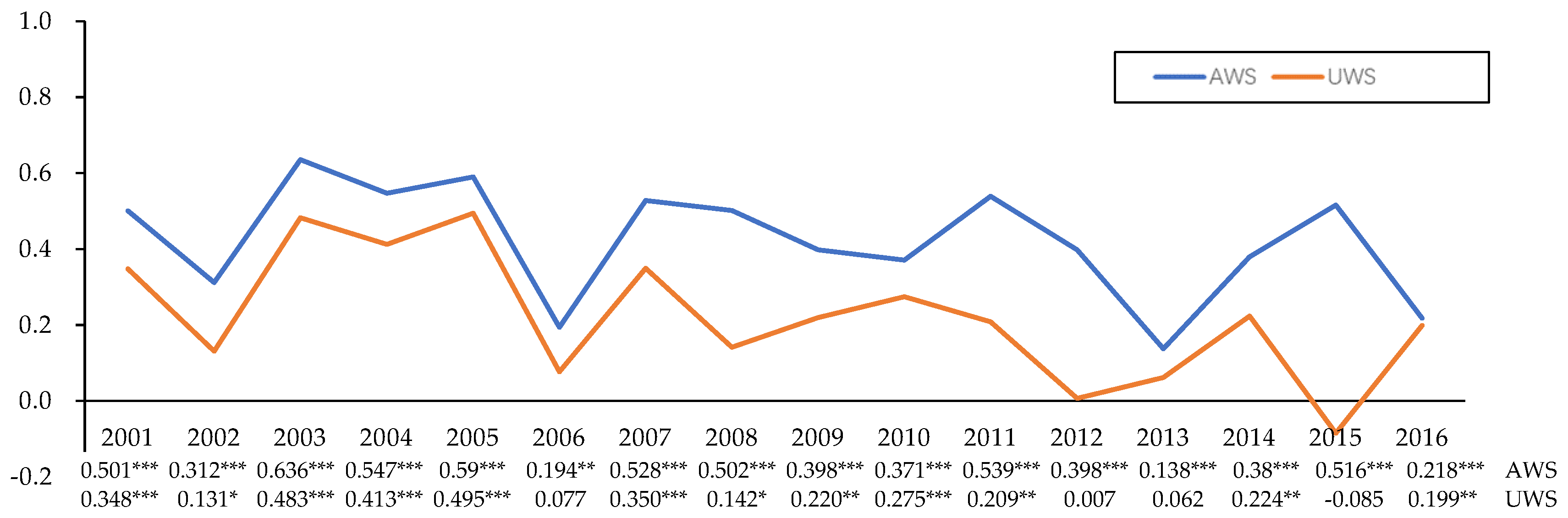
Figure 3 shows Global Moran’s I. It shows that both agricultural and UWS have a positive significant correlation across the cities in most years over the studied period. The high value represents the high degree of spatial correlation. AWS had a significant spatial correlation every year. Regarding the UWS, some years did not have a significant spatial autocorrelation as in 2006, 2012, 2013, and 2015. After 2010, this trend became more apparent, and three years did not have spatial autocorrelation.
4.2. Model Estimation
Table 3 shows 6 models, which include the fixed-effect (FE) and random effect (RE) versions of SAR, SEM, and SDM model. The LM test found that SDM models are more appropriate. In panel data analysis, regional characteristic variables could not be used in the fixed-effects models. It will have multi-collinearity. Auci and Vignani (2021) consider the limitations of the fixed-effect model in agricultural water studies. Since we focused on regional characteristics, we selected random effect models. Next, SDM RE was selected for explanations.
As shown in Table 3, among the main variables, traditional plant areas, vegetable plant areas, agricultural population, UWS, precipitation, and temperature have significant effects on AWS. The increase in traditional plant areas has led to increased AWS in SAR SEM, and SDM. In the SDM RE model, traditional and vegetable plant areas’ coefficients are 0.127 and 0.354, respectively. Thus, traditional planting causes less impact than vegetable planting to the local water environment. Agricultural population coefficient is 0.175, UWS coefficient is 0.222, precipitation coefficient is −1.125, and temperature coefficient is −2.411. All of them have significant effects on AWS.
As for the spatial variable, we report significant variables only in Table 3. An increase in neighborhood AWS leads to an increase in AWS. Neighborhood agricultural factors significantly affect AWS. An increase in neighborhood agriculture population leads to increased AWS. In SDM RE model, Neighborhood AWS coefficient is 0.275 and neighborhood agriculture population coefficient is 0.261.
Marginal effects are shown in Table 4. The direct effect refers to the impacts due to the area’s own variables. The indirect effect refers to the impacts due to the variables in neighborhood areas. The total effect sums up these two effects for each variable. As shown in Table 4, the agricultural population has a significant positive effect in both direct and indirect effects. Agricultural population coefficient is 0.597 in the total effect. Different plant structures have a significant effect on AWS. However, it has only a direct impact, and the indirect impact is not significant. Traditional plant areas coefficient is 0.349 in the direct effect.
4.3. Robustness of Results
In the robustness test, we use the spatial matrix of inverse-distance matrix instead of the adjacency matrix. The inverse distance matrix is the reciprocal matrix of the distance from the center of city. We re-estimate the SDM. The results shown in Table 5 are similar to the binary adjacency matrix estimates. This robustness test result verifies the accuracy of the spatial influence so far described.
5. Discussion
We used spatial analysis approach consisting of three parts: the Global Moran index, the spatial analysis of the influencing factors, and the robustness test. UWS has spatial correlation with the UWS of neighboring areas when viewed by the Moran’s I. Agriculture water supply internalization showed spatial correlations with neighborhood values both with Global Moran’s I and spatial models.
5.1. Agricultural Development and AWS
To answer our first research question, we studied the impacts of agricultural development on agricultural water using spatial models (see Table 3). Regarding the direct effects, agricultural population affects AWS. Agricultural economy’s efficiency increases under migration from agricultural areas to cities [4] and, thus, decreasing agricultural population can reflect a modern agricultural development pattern. We found that an agricultural population decrease leads to a decrease in AWS meaning more efficient use of agricultural water per regional water resources. Thus, a modern agriculture development pattern is beneficial to sustaining the water environment.
The direct effect on AWS may be relieved by adjusting crop types. Our analysis showed that traditional crop planting reduces agricultural water internalization relative to vegetable planting and thus traditional crop planting poses less threat to the local water environment. Auci (2021) found no significant impact of crop typology on irrigation water consumption, which is different from our findings. The difference may be attributable to the definitions of crop typology. Auci (2021) focuses on local specialty crops, and studied Citrus, Grapevine, Olive, vegetables, fruits, and so on. We aimed to study the impact of different cultivation techniques on agricultural water use from a technological point of view, in an industry where agricultural technology conversion is relatively easy to accept. We used the structure of types of crops rather than individual crops. We used traditional plant areas and vegetable areas. In addition, we used spatial models. Thus, we obtained different results.
Regarding the indirect effects or spatial correlations, neighborhood cities’ AWS affects own AWS. Neighborhood cities’ agricultural populations also affects own AWS. The latter result may be caused by agricultural population agglomeration. Agricultural population agglomeration refers to neighborhood cities’ agricultural populations sharing a similar trend. Neighborhood areas tend to have similar agricultural population phenomena because of their similar development patterns and population mobility.
5.2. Urbanization and AWS
Urban development may need to utilize water resources that were used for agriculture, as stated in our second research question. We analyzed this issue from multiple perspectives. Our spatial models in Table 3 shows that UWS has a positive direct effect to AWS. Thus, when urban water consumption pressure is high in a city, the consumption pressure on agricultural water use is also high in the same city. This result may be consistent with the view that these two sectors are competing over water.
Regarding the indirect effects, Figure 3 showed that AWS and UWS had similar trending patterns. Thus, when spatial correlation is high in terms of AWS, it is also high in terms of UWS. However, this relationship may have been weakened recently as was seen in 2015. Then, as a cluster of cities in a large area, the levels of water competition between the urban and agricultural sectors may have eased. The special correlation between AWS and UWS was not identified in the spatial models. We think that this is because climate conditions are controlled in the spatial models. AWS is more affected by climate and in the same climatic zone, AWS should show a stronger aggregation effect. UWS is less affected by climate and its aggregation effect is less obvious.
5.3. Climate Factors
AWS is largely affected by the climate of own area and neighborhood cities. Different water supply internalizations have essential connections with climatic factors. We found that precipitation decreases AWS. In general, suitable precipitation has a positive impact. High temperature areas show low levels of AWS. Temperature has different signs between the direct and indirect effects and needs further studies to determine the reason for the different signs.
5.4. Policy Suggestions
To reduce impact to the local water environment, the agriculture sector needs to enhance agricultural patterns and improve technology. Mensah (2019) emphasized the importance of agricultural technology. As shown in Table 3, there are two methods to enhance agriculture pattern. First, agriculture could decrease the agricultural population. Second, plant structure adjusting is useful. Suitable agricultural strategies and transformation to urban service-oriented agriculture should be pursued.
In terms of the relationship with urban areas, urban and agricultural water use needs to be balanced under integrated water resource management (IWRM). The increase in UWS has both natural and anthropogenic connections with AWS. It needs integrated management of different water sectors. The Global Water Partnership (GWP, 2000) defines IWRM as “a process which promotes the coordinated development and management of water, land, and related resources to maximize the resultant economic and social welfare equitably without compromising the sustainability of vital ecosystems” [41].
In terms of regional aggregation, the government should encourage agricultural cooperation across areas. It strengthens regional agricultural cooperation to promote agricultural development and reduce environmental harm. As shown in Table 3, AWS has spatial agglomeration. Agglomeration of agricultural factors bring more pressure to AWS. Agglomeration of agricultural factors has a positive effect on agriculture. Regional cooperation should also be strengthened, such as agriculture and water saving cooperation.
6. Conclusions
We found from our series of spatial analysis that agricultural development affects AWS, which shows the impact of agricultural water use on the local water environment. There are two kinds of effects. Agricultural development in own area directly affects AWS. A decrease in the agricultural population reduces AWS. Agricultural spatial distribution indirectly affects AWS. Increased agriculture population and other factors in neighborhood cities increase AWS in own city. Regarding the impact of urbanization, UWS affects AWS directly. Effective regional cooperation is needed to reduce impacts to the local water environment. To answer the remaining questions, influential factors need to be further studied.
Author Contributions
Conceptualization, M.S.; methodology, M.S.; validation, T.K.; formal analysis, M.S.; investigation, M.S.; resources, T.K.; data curation, M.S.; writing—original draft preparation, M.S.; writing—review and editing, T.K.; supervision, T.K.; project administration, T.K.; funding acquisition, T.K. All authors have read and agreed to the published version of the manuscript.
Funding
This work was supported by the Student Research Fund of the University of Kitakyushu.
Institutional Review Board Statement
Ethical review and approval were waived for this study, due to its use of publicly available government statistics as its data source.
Informed Consent Statement
Not applicable.
Data Availability Statement
The data used for this research are available from the authors upon request.
Conflicts of Interest
The authors declare no conflict of interest.
References
- Flörke, M.; Schneider, C.; McDonald, R.I. Water competition between cities and agriculture driven by climate change and urban growth. Nat. Sustain. 2018, 1, 51–58. [Google Scholar] [CrossRef]
- Chartzoulakis, K.; Bertaki, M. Sustainable water management in agriculture under climate change. Agric. Agric. Sci. Procedia 2015, 4, 88–98. [Google Scholar] [CrossRef]
- Falkenmark, M. Eco-conflicts-the water cycle perspective. Environ. Confl. Proj. Occas. Rep. 1995, 14, 31–47. [Google Scholar]
- Siciliano, G. Urbanization strategies, rural development and land use changes in China: A multiple-level integrated assessment. Land Use Policy 2012, 29, 165–178. [Google Scholar] [CrossRef]
- Auci, S.; Vignani, D. Irrigation water intensity and climate variability: An agricultural crops analysis of Italian regions. Environ. Sci. Pollut. Res. 2021, 28, 63794–63814. [Google Scholar] [CrossRef]
- Zhao, C.; Chen, B.; Hayat, T.; Alsaedi, A.; Ahmad, B. Driving force analysis of water footprint change based on extended STIRPAT model: Evidence from the Chinese agricultural sector. Ecol. Indic. 2014, 47, 43–49. [Google Scholar] [CrossRef]
- Gebre, T.; Gebremedhin, B. The mutual benefits of promoting rural-urban interdependence through linked ecosystem services. Glob. Ecol. Conserv. 2019, 20, e00707. [Google Scholar] [CrossRef]
- Jiang, Y. China’s water scarcity. J. Environ. Manag. 2009, 90, 3185–3196. [Google Scholar] [CrossRef]
- Meng, C.; Wang, X.; Li, Y. An optimization model for water management based on water resources and environmental carrying capacities: A case study of the Yinma River Basin, Northeast China. Water 2018, 10, 565. [Google Scholar] [CrossRef]
- Wang, J.; Li, Y.; Huang, J.; Yan, T.; Sun, T. Growing water scarcity, food security and government responses in China. Glob. Food Sec. 2017, 14, 9–17. [Google Scholar] [CrossRef]
- Jia, Z.; Cai, Y.; Chen, Y.; Zeng, W. Regionalization of water environmental carrying capacity for supporting the sustainable water resources management and development in China. Resour. Conserv. Recycl. 2018, 134, 282–293. [Google Scholar] [CrossRef]
- Falkenmark, M.; Berntell, A.; Jägerskog, A.; Lundqvist, J.; Matz, M.; Tropp, H. On the Verge of a New Water Scarcity: A Call for Good Governance and Hyman Ingenuity; Stockholm International Water Institute (SIWI): Stockholm, Sweden, 2007; pp. 1–19. [Google Scholar]
- Falkenmark, M.; Molden, D. Wake up to realities of river basin closure. Int. J. Water Resour. Dev. 2008, 24, 201–215. [Google Scholar] [CrossRef]
- Renouf, M.A.; Serrao-Neumann, S.; Kenway, S.J.; Morgan, E.A.; Choy, D.L. Urban water metabolism indicators derived from a water mass balance–bridging the gap between visions and performance assessment of urban water resource management. Water Res. 2017, 122, 669–677. [Google Scholar] [CrossRef] [PubMed]
- Billings, S.B.; Johnson, E.B. Agglomeration within an urban area. J. Urban. Econ. 2016, 91, 13–25. [Google Scholar] [CrossRef]
- Zhong, C.; Hu, R.; Wang, M.; Xue, W.; He, L. The impact of urbanization on urban agriculture: Evidence from China. J. Clean. Prod. 2020, 276, 122686. [Google Scholar] [CrossRef]
- Wang, F.; Yu, C.; Xiong, L.; Chang, Y. How can agricultural water use efficiency be promoted in China? A spatial-temporal analysis. Resour. Conserv. Recycl. 2019, 145, 411–418. [Google Scholar] [CrossRef]
- Mu, L.; Fang, L.; Dou, W.; Wang, C.; Qu, X.; Yu, Y. Urbanization-induced spatio-temporal variation of water resources utilization in northwestern China: A spatial panel model based approach. Ecol. Indic. 2021, 125, 107457. [Google Scholar] [CrossRef]
- Dethier, J.-J.; Eenberger, A. Agriculture and development: A brief review of the literature. Econ. Syst. 2012, 36, 175–205. [Google Scholar] [CrossRef]
- Li, J.; Fei, L.; Li, S.; Xue, C.; Shi, Z.; Hinkelmann, R. Development of “water-suitable” agriculture based on a statistical analysis of factors affecting irrigation water demand. Sci. Total Environ. 2020, 744, 140986. [Google Scholar] [CrossRef]
- Galioto, F.; Chatzinikolaou, P.; Raggi, M.; Viaggi, D. The value of information for the management of water resources in agriculture: Assessing the economic viability of new methods to schedule irrigation. Agric. Water Manag. 2020, 227, 105848. [Google Scholar] [CrossRef]
- Song, M.; Wang, R.; Zeng, X. Water resources utilization efficiency and influence factors under environmental restrictions. J. Clean. Prod. 2018, 184, 611–621. [Google Scholar] [CrossRef]
- Xinchun, C.; Mengyang, W.; Xiangping, G.; Yalian, Z.; Yan, G.; Nan, W.; Weiguang, W. Assessing water scarcity in agricultural production system based on the generalized water resources and water footprint framework. Sci. Total Environ. 2017, 609, 587–597. [Google Scholar] [CrossRef] [PubMed]
- Kendy, E.; Wang, J.; Molden, D.J.; Zheng, C.; Liu, C.; Steenhuis, T.S. Can urbanization solve inter-sector water conflicts? Insight from a case study in Hebei Province, North China Plain. Water Policy 2007, 9, 75–93. [Google Scholar] [CrossRef]
- Mohan, G.; Chapagain, S.K.; Fukushi, K.; Papong, S.; Sudarma, I.M.; Rimba, A.B.; Osawa, T. An extended input–output framework for evaluating industrial sectors and provincial-level water consumption in Indonesia. Water Resour. Ind. 2021, 25, 100141. [Google Scholar] [CrossRef]
- Antoci, A.; Borghesi, S.; Sodini, M. Water resource use and competition in an evolutionary model. Water Resour. Manag. 2017, 31, 2523–2543. [Google Scholar] [CrossRef]
- Falkenmark, M. The massive water scarcity now threatening Africa: Why isn’t it being addressed? Ambio 1989, 18, 112–118. [Google Scholar]
- Falkenmark, M.; Widstrand, C. Population and water resources: A delicate balance. Popul. Bull. 1992, 47, 1–36. [Google Scholar]
- Tang, H. Comparative analysis of wheat production capacity in major production areas. J. Henan Agric. Sci. 2008, 6, 4. (In Chinese) [Google Scholar]
- Govere, S.; Nyamangara, J.; Nyakatawa, E.Z. Climate change signals in the historical water footprint of wheat production in Zimbabwe. Sci. Total Environ. 2020, 742, 140473. [Google Scholar] [CrossRef]
- He, L.; Du, Y.; Wu, S.; Zhang, Z. Evaluation of the agricultural water resource carrying capacity and optimization of a planting-raising structure. Agric. Water Manag. 2021, 243, 106456. [Google Scholar] [CrossRef]
- Hoekstra, A.Y.; Chapagain, A.K.; Aldaya, M.M.; Mekonnen, M.M. The Water Footprint Assessment Manual: Setting the Global Standard; Earth Scan Press: London, UK, 2011. [Google Scholar]
- Chen, Z.; Song, S. Efficiency and technology gap in China’s agriculture: A regional meta-frontier analysis. China Econ. Rev. 2008, 19, 287–296. [Google Scholar] [CrossRef]
- Petrescu-Mag, R.M.; Petrescu, D.C.; Reti, K.-O. My land is my food: Exploring social function of large land deals using food security–land deals relation in five Eastern European countries. Land Use Policy 2019, 82, 729–741. [Google Scholar] [CrossRef]
- Paelinck, J.H.P.; Klaassen, L.H. Spatial Econometrics; Saxon House: Farnborough, UK, 1979. [Google Scholar]
- Deng, X.J.; Xu, Y.P.; Han, L.F.; Yang, M.N.; Yang, L.; Song, S.; Li, G.; Wang, Y.F. Spatial-temporal evolution of the distribution pattern of river systems in the plain river network region of the Taihu Basin, China. Quat. Int. 2016, 392, 178–186. [Google Scholar] [CrossRef]
- Wang, Z.Y.; Cheng, Y.Q.; Ye, X.Y.; Wei, Y.H.D. Analyzing the space-time dynamics of innovation in China: ESDA and spatial panel approaches. Growth Chang. 2016, 47, 111–129. [Google Scholar] [CrossRef]
- Elhorst, J.P. Spatial Panel Data Analysis. Encycl. GIS 2017, 2, 2050–2058. [Google Scholar]
- LeSage, J.; Pace, R.K. Introduction to Spatial Econometrics; CRC Press: Boca Raton, FL, USA, 2009; pp. 113–145. [Google Scholar]
- Lee, L.F. Consistency and efficiency of least squares estimation for mixed regressive, spatial autoregressive models. Econom. Theory 2002, 18, 252–277. [Google Scholar] [CrossRef]
- Global Water Partnership (GWP). Integrated Water Resources Management. TAC Background Paper 4. Glob. Water Partnersh. Stockh. 2000. Available online: https://www.gwp.org/globalassets/global/toolbox/publications/background-papers/04-integrated-water-resources-management-2000-english.pdf (accessed on 1 August 2022).
Figure 1.
Locations of the urban center of the 30 cities in four provinces.

Figure 2.
Model structure.

Figure 3.
Trends in Global Moran’s I. * 10% significance, ** 5% significance, *** 1% significance.


Table 1.
Water supply internalization indicators.
| Name and Abbreviation | Definition | Mean | Standard Deviation | Max | Min |
|---|---|---|---|---|---|
| Agricultural water (AW) | Amount of water supplied to the agricultural industry within a city boundary (100 million m3) | 10.759 | 6.149 | 29.21 | 1.000 |
| Urban water (UW) | Amount of urban and industrial water supply among the total water supply in the boundary (100 million m3) | 5.031 | 4.439 | 32.7 | 0.131 |
| water resource (WR) | Amount of nature water within the city boundary (100 million m3) | 15.538 | 11.126 | 86.76 | 0.71 |
| Urban water supply internalization (UWS) | Ratio of urban water supply against local nature water supply (m3/m3) | 0.452 | 0.442 | 5.104 | 0.009 |
| Agricultural water supply internalization (AWS) | Ratio of agricultural water supply against local nature water supply (m3/m3) | 1.070 | 1.259 | 11.944 | 0.058 |
Table 2.
Independent variables.
| Variable Abbreviation | Variable Name and Definition | Mean | Standard Deviation | Max | Min |
|---|---|---|---|---|---|
| agr1 | Agricultural population (10,000 person) | 369.939 | 199.802 | 940.028 | 53.491 |
| agr2 | Agricultural GDP (100 million yuan) | 4.938 | 0.037 | 598.98 | 1.589 |
| agr3 | Agricultural machine power (10,000 kilowatts) | 9019.674 | 128,920.9 | 2,000,000 | 68.891 |
| agr4 | Vegetable planting areas (1000 hectares) | 438,778.149 | 5,251,670 | 278,637 | 16,172 |
| agr5 | Traditional plant planting areas (1000 hectares) | 172,560.534 | 5,298,969 | 1,300,000 | 39,512.3 |
| C1 | Climate factor Temperature (°C) | 12.714 | 1.243 | 14.821 | 8.069 |
| C2 | Climate factor Precipitation (100 million m3) | 69.445 | 39.536 | 236.3 | 10.1 |
| L | Water accessibility (4 levels) | 2 | 1.001 | 4 | 1 |
Note: GDP—Gross Domestic Product.
Table 3.
Model estimate.
| Variables | SAR | SEM | SDM | |||
|---|---|---|---|---|---|---|
| FE | RE | FE | RE | FE | RE | |
| Spatial correlation: | ||||||
| ln (Agricultural water supply internalization) | 0.243 *** | 0.288 *** | 0.251 *** | 0.275 *** | ||
| (0.000) | (0.000) | (0.000) | (0.000) | |||
| Ln | 0.287 *** | 0.302 *** | ||||
| (0.000) | (0.000) | |||||
| ln (Agricultural population) | 0.429 *** | 0.261 ** | ||||
| (0.003) | (0.052) | |||||
| ln (vegetable areas) | −0.183 * | −0.109 | ||||
| (0.059) | (0.267) | |||||
| ln (Water accessibility) | 0.649 * | |||||
| (0.076) | ||||||
| Main variables: | ||||||
| ln (Agricultural population) | 0.227 *** | 0.252 *** | 0.227 ** | 0.290 *** | 0.010 | 0.175 * |
| (0.003) | (0.001) | (0.012) | (0.001) | (0.927) | (0.057) | |
| ln (Agricultural GDP) | −0.029 * | −0.026 | −0.036 * | −0.032 | 0.029 | 0.024 |
| (0.105) | (0.163) | (0.105) | (0.154) | (0.366) | (0.468) | |
| ln (Agricultural machine power) | 0.002 | 0.006 | 0.006 | −0.002 | 0.006 | 0.008 |
| (0.912) | (0.842) | (0.701) | (0.930) | (0.701) | (0.646) | |
| ln (Traditional plant areas) | 0.049 | 0.337 *** | 0.187 *** | 0.165 ** | −0.087 | 0.127 ** |
| (0.749) | (0.005) | (0.004) | (0.013) | (0.606) | (0.059) | |
| ln (Vegetable areas) | 0.181 *** | 0.164 *** | 0.095 | 0.412 *** | 0.146 ** | 0.354 *** |
| (0.003) | (0.006) | (0.558) | (0.003) | (0.031) | (0.008) | |
| ln (Precipitation) | −1.232 *** | −1.081 *** | −1.483 *** | −1.387 *** | −1.275 *** | −1.125 *** |
| (0.000) | (0.000) | (0.000) | (0.000) | (0.000) | (0.000) | |
| ln (Temperature) | 0.165 | −0.036 | 0.608 | 0.389 | −2.654 *** | −2.411 ** |
| (0.660) | (0.921) | (0.211) | (0.430) | (0.000) | (0.017) | |
| ln (Water accessibility) | 0.068 | 0.168 | −0.402 | |||
| (0.703) | (0.461) | (0.163) | ||||
| ln (Urban water supply internalization) | 0.196 *** | 0.223 *** | 0.219 *** | 0.246 *** | 0.205 *** | 0.222 *** |
| (0.000) | (0.000) | (0.000) | (0.000) | (0.000) | (0.000) | |
| Constant | −3.169 * | −4.273 | −0.138 | |||
| (0.070) | (0.049) | (0.965) | ||||
| R2 | 0.821 | 0.817 | 0.814 | 0.812 | 0.833 | 0.828 |
| LM test | 209.061 *** | 101.083 *** | ||||
| (0.000) | (0.000) |
Note: GDP—Gross Domestic Product; * 10% significance, ** 5% significance, *** 1% significance, p-values in parentheses.
Table 4.
Average marginal effects by SDM RE.
| Direct Effect | Indirect Effect | Total Effect | |
|---|---|---|---|
| ln (Agricultural population) | 0.201 ** | 0.396 ** | 0.597 *** |
| (0.029) | (0.010) | (0.000) | |
| ln (Agricultural GDP) | 0.02 | −0.046 | −0.026 |
| (0.504) | (0.304) | (0.437) | |
| ln (Agricultural machine power) | 0.008 | −0.005 | 0.002 |
| (0.656) | (0.932) | (0.970) | |
| ln (Traditional plant areas) | 0.349 *** | −0.318 | 0.031 |
| (0.006) | (0.259) | (0.918) | |
| ln (Vegetable areas) | 0.118 ** | −0.085 | 0.033 |
| (0.056) | (0.495) | (0.807) | |
| ln (Precipitation) | −1.144 *** | −0.317 *** | −1.461 *** |
| (0.000) | (0.040) | (0.000) | |
| ln (Temperature) | −2.187 ** | 2.929 *** | 0.742 |
| (0.020) | (0.007) | (0.154) | |
| ln (Water assess way) | −0.334 | 0.648 * | 0.315 |
| (0.217) | (0.095) | (0.314) | |
| ln (Urban water supply internalization) | 0.226 *** | 0.084 | 0.31 *** |
| (0.000) | (0.151) | (0.000) |
Note: * 10% significance, ** 5% significance, *** 1% significance, p-values in parentheses.
Table 5.
Robustness test for SDM RE.
| Direct Effect | Indirect Effect | Total Effect | |
|---|---|---|---|
| ln (Agricultural population) | 0.296 *** | 0.592 * | 0.888 *** |
| (0.003) | (0.076) | (0.010) | |
| ln (Agricultural GDP) | 0.005 | −0.052 | −0.046 |
| (0.845) | (0.480) | (0.458) | |
| ln (Agricultural machine power) | 0.002 | 0.165 | 0.179 |
| (0.970) | (0.381) | (0.354) | |
| ln (Traditional plant areas) | 0.47 *** | −1.595 | −1.125 |
| (0.001) | (0.114) | (0.280) | |
| ln (Vegetable areas) | 0.039 | −0.068 | −0.03 |
| (0.553) | (0.839) | (0.930) | |
| ln (Precipitation) | −1.318 *** | 0.212 | −1.106 ** |
| (0.000) | (0.651) | (0.024) | |
| ln (Temperature) | −1.549 * | 2.199 * | 0.65 |
| (0.056) | (0.081) | (0.438) | |
| ln (Water assess way) | −0.266 | 0.234 | 1.315 |
| (0.301) | (0.259) | (0.437) | |
| ln (Urban water supply internalization) | 0.253 *** | 1.58 | 0.487 ** |
| (0.000) | (0.382) | (0.023) |
Note: * 10% significance, ** 5% significance, *** 1% significance, p-values in parentheses.
Publisher’s Note: MDPI stays neutral with regard to jurisdictional claims in published maps and institutional affiliations. |
© 2022 by the authors. Licensee MDPI, Basel, Switzerland. This article is an open access article distributed under the terms and conditions of the Creative Commons Attribution (CC BY) license (https://creativecommons.org/licenses/by/4.0/).
Share and Cite
MDPI and ACS Style
Sun, M.; Kato, T. The Effect of Urban Agriculture on Water Security: A Spatial Approach. Water 2022, 14, 2529. https://doi.org/10.3390/w14162529
AMA Style
Sun M, Kato T. The Effect of Urban Agriculture on Water Security: A Spatial Approach. Water. 2022; 14(16):2529. https://doi.org/10.3390/w14162529
Chicago/Turabian StyleSun, Menglu, and Takaaki Kato. 2022. "The Effect of Urban Agriculture on Water Security: A Spatial Approach" Water 14, no. 16: 2529. https://doi.org/10.3390/w14162529
Note that from the first issue of 2016, this journal uses article numbers instead of page numbers. See further details here.