
A Comparative Evaluation of Conceptual Rainfall–Runoff Models for a Catchment in Victoria Australia Using eWater Source

 , , ,
, , ,
Abstract
:1. Introduction
2. Methodology
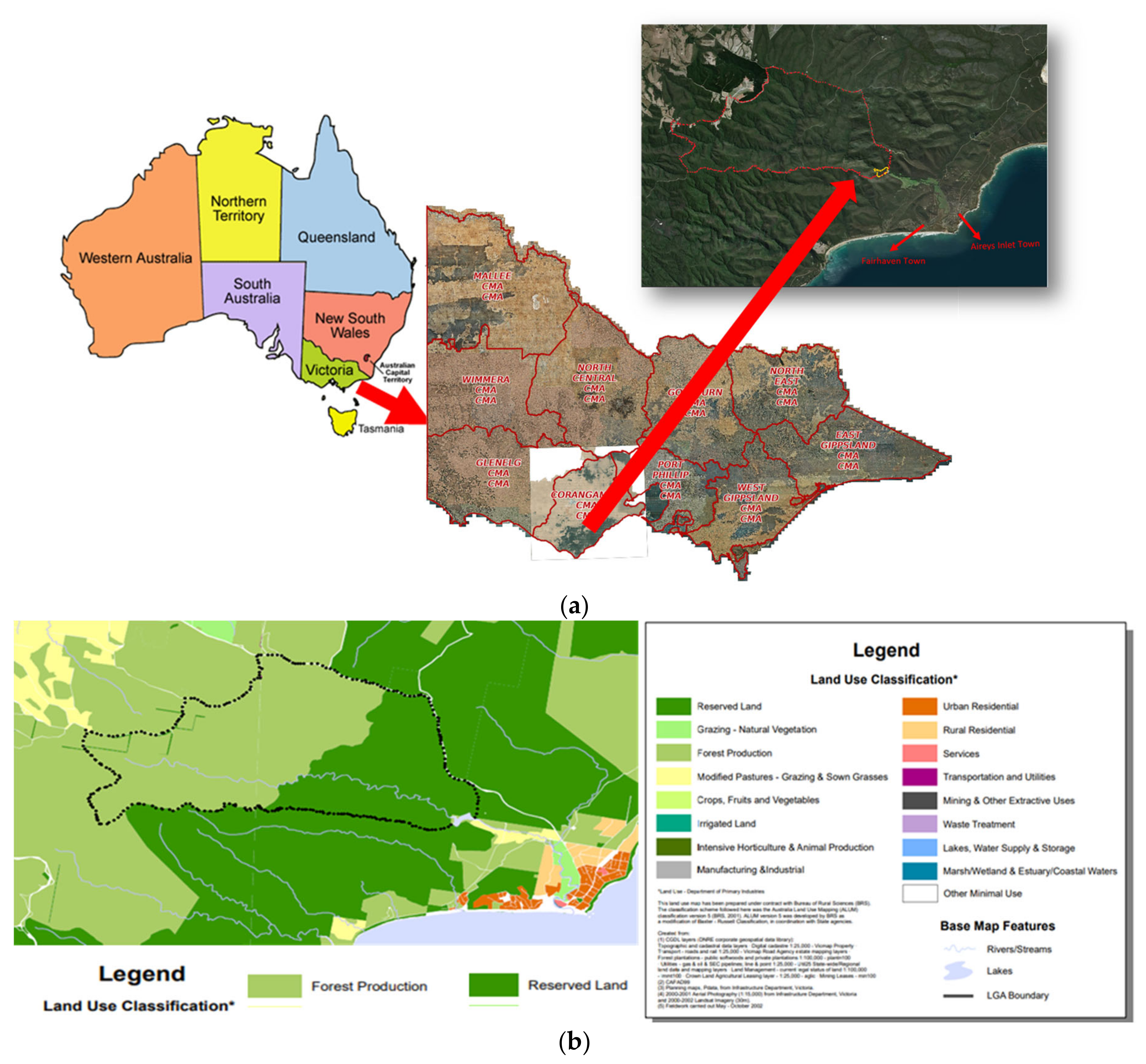
2.1. Study Area
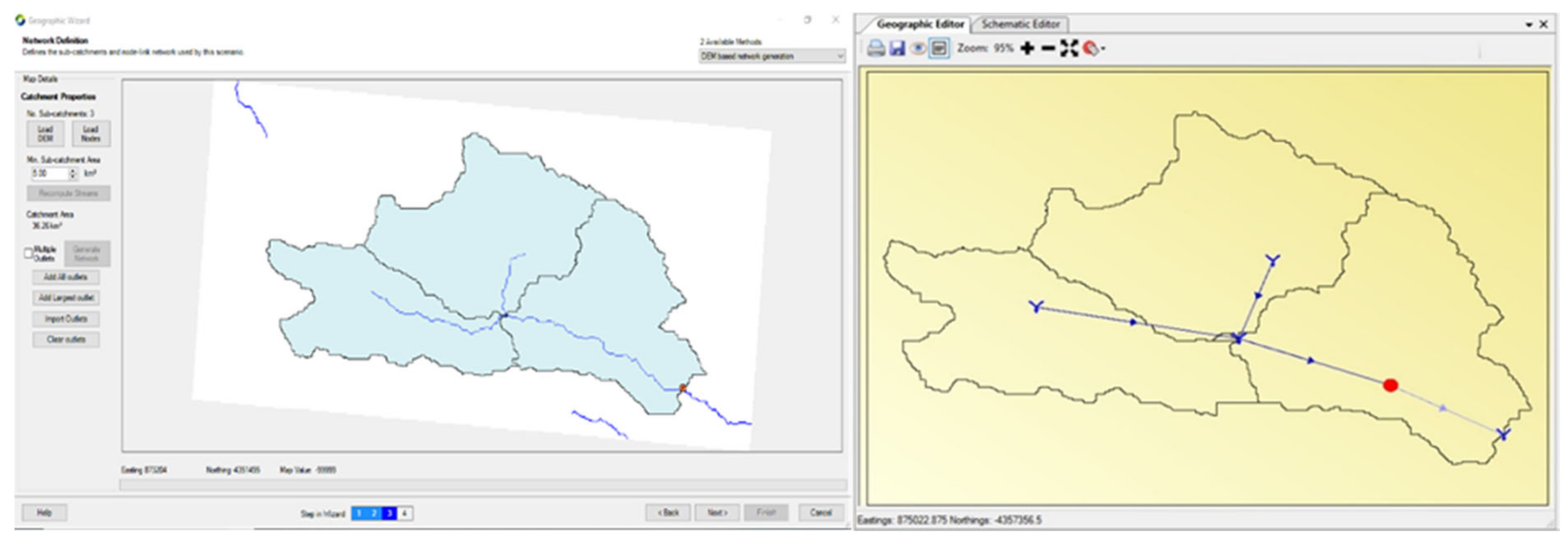
2.2. Source Model Catchment Configuration
2.2.1. GR4J Model
2.2.2. Australian Water Balance Model (AWBM)
2.2.3. Sacramento Rainfall–Runoff Model
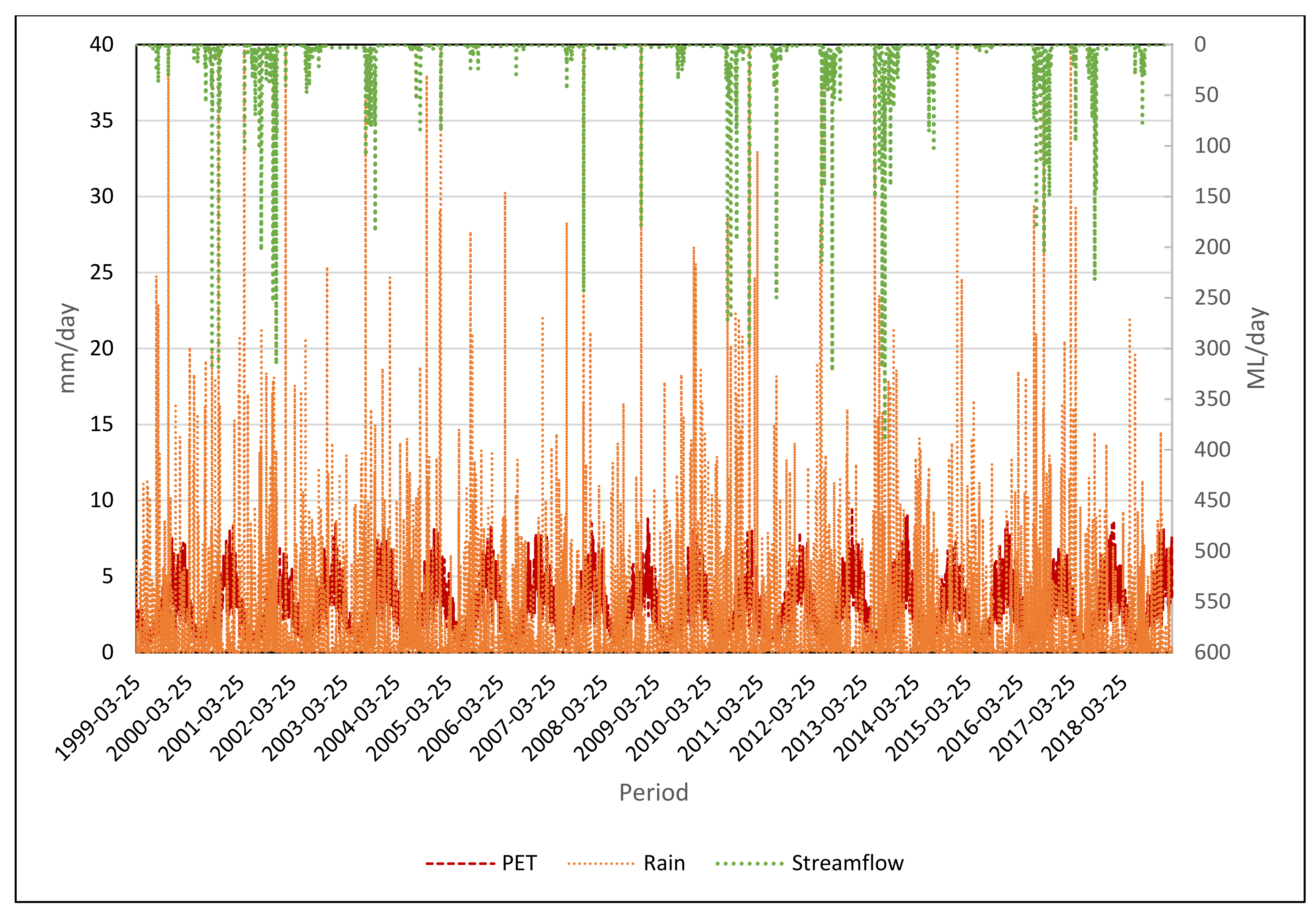
2.3. Catchment, Streamflow and Climate Data
2.4. Model Calibration and Validation
3. Model Results
3.1. Calibration and Validation of Selected Models
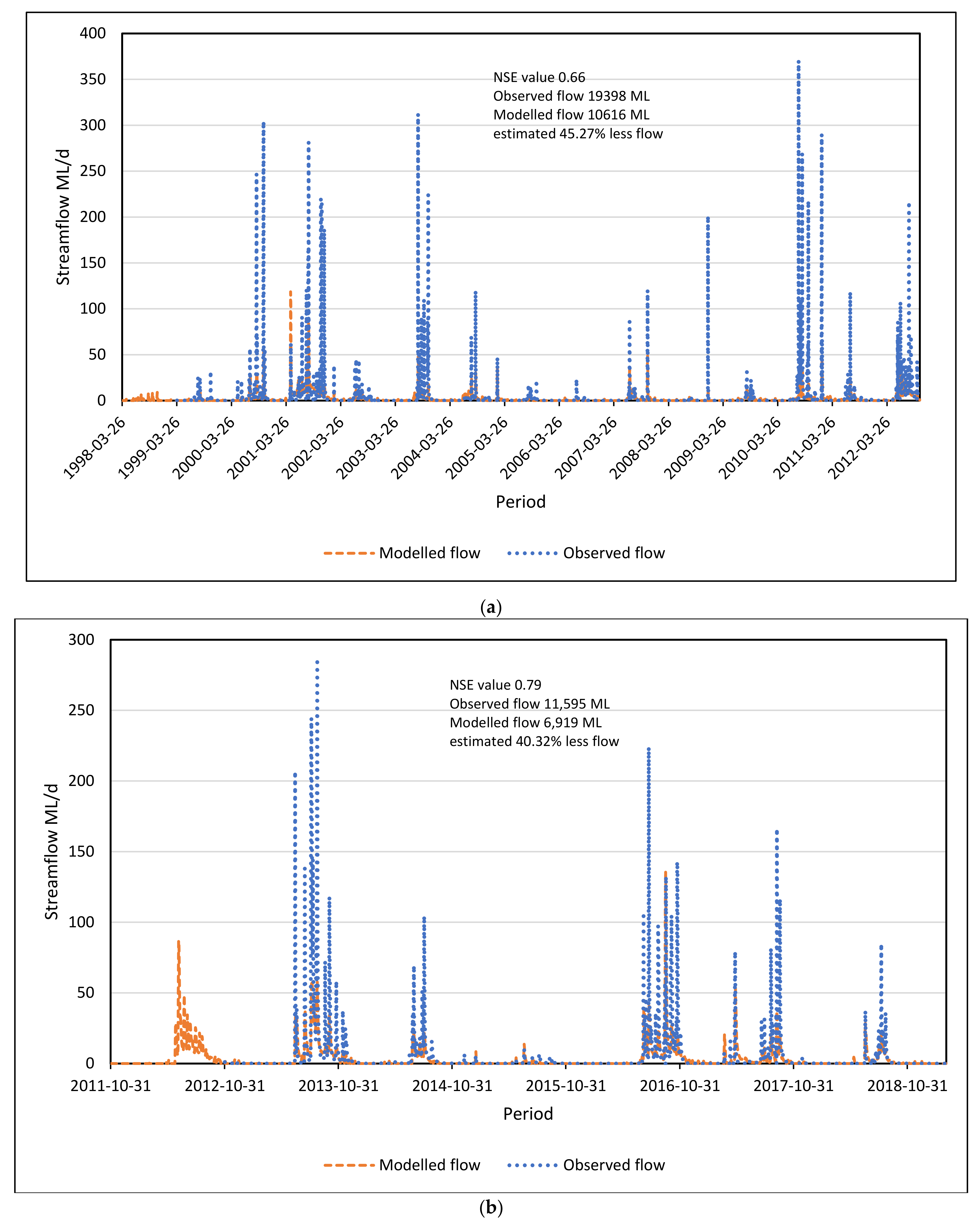
3.1.1. AWBM Model Calibration and Validation
3.1.2. Sacramento Model Calibration and Validation
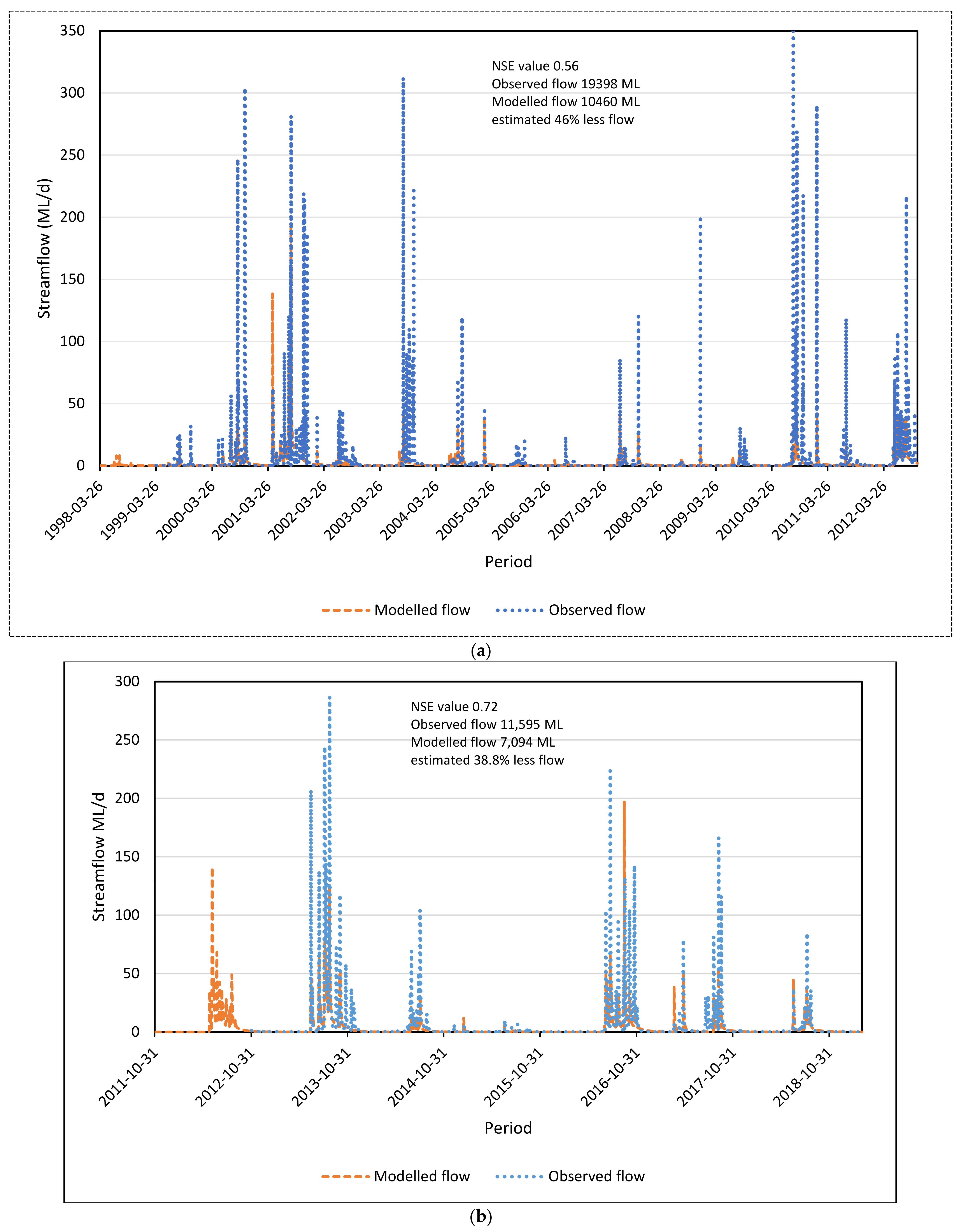
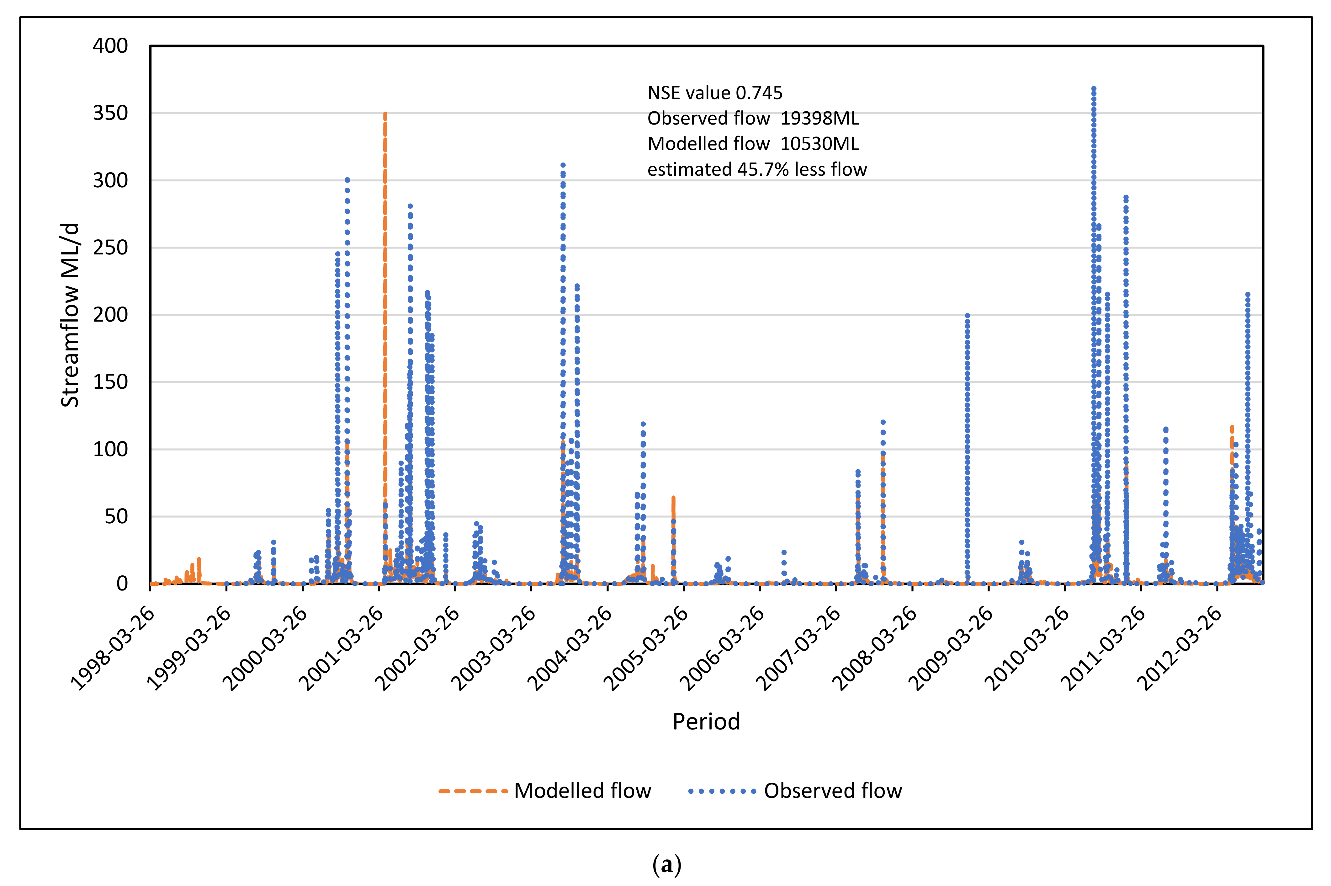
3.1.3. GR4J Model Calibration and Validation
3.2. GR4J Model Application under Different Scenarios
- (A)
- Land use change in the case study catchment from forest land to agricultural land use.
- (B)
- Climate change impacts.
- (C)
- Combined land use and climate change impacts.
3.2.1. Land Use Change Impact
3.2.2. Higher Climate Change Scenario
3.2.3. Combined Land-Use and Higher Climate Change Scenario
4. Conclusions
Author Contributions
Funding
Institutional Review Board Statement
Informed Consent Statement
Data Availability Statement
Acknowledgments
Conflicts of Interest
References
- Vaze, J.; Chiew, F.; Perraud, J.-M.; Viney, N.; Post, D.; Teng, J.; Wang, B.; Lerat, J.; Goswami, M. Rainfall-runoff modelling across southeast Australia: Datasets, models and results. Australas. J. Water Resour. 2011, 14, 101–116. [Google Scholar] [CrossRef]
- De Vos, N.; Rientjes, T. Multi-objective performance comparison of an artificial neural network and a conceptual rainfall—Runoff model. Hydrol. Sci. J. 2007, 52, 397–413. [Google Scholar] [CrossRef]
- Dwarakish, G.; Ganasri, B. Impact of land use change on hydrological systems: A review of current modeling approaches. Cogent Geosci. 2015, 1, 1115691. [Google Scholar] [CrossRef]
- DELWP. Guidelines for Assessing the Impact of Climate Change on Water Supplies in Victoria. 2016. Available online: https://www.water.vic.gov.au/__data/assets/pdf_file/0014/52331/Guidelines-for-Assessing-the-Impact-of-Climate-Change-on-Water-Availability-in-Victoria.pdf (accessed on 13 April 2021).
- Legesse, D.; Vallet-Coulomb, C.; Gasse, F. Hydrological response of a catchment to climate and land use changes in Tropical Africa: Case study South Central Ethiopia. J. Hydrol. 2003, 275, 67–85. [Google Scholar] [CrossRef]
- Leavesley, G.H. Modeling the effects of climate change on water resources—A review. Assess. Impacts Clim. Chang. Nat. Resour. Syst. 1994, 28, 159–177. [Google Scholar]
- Kunnath-Poovakka, A.; Eldho, T. A comparative study of conceptual rainfall-runoff models GR4J, AWBM and Sacramento at catchments in the upper Godavari river basin, India. J. Earth Syst. Sci. 2019, 128, 33. [Google Scholar] [CrossRef]
- Chiew, F.; Peel, M.; Western, A. Application and testing of the simple rainfall-runoff model SIMHYD. In Mathematical Models of Small Watershed Hydrology and Applications; Water Resources Publications: Highlands Ranch, CO, USA, 2002; pp. 335–367. Available online: https://wrpllc.com/books/mmsw.html (accessed on 30 June 2022).
- Carr, R.; Podger, G. eWater Source-Australia’s next generation IWRM modelling platform. In Proceedings of the Hydrology and Water Resources Symposium 2012, Sydney, NSW, Australia, 19–22 November 2012; p. 742. [Google Scholar]
- Dutta, D.; Welsh, W.D.; Vaze, J.; Kim, S.S.; Nicholls, D. A comparative evaluation of short-term streamflow forecasting using time series analysis and rainfall-runoff models in eWater source. Water Resour. Manag. 2012, 26, 4397–4415. [Google Scholar] [CrossRef]
- Vaze, J.; Jordan, P.; Beecham, R.; Frost, A.; Summerell, G. Guidelines for Rainfall-Runoff Modelling: Towards Best Practice Model Application; eWater CRC: Clayton, VIC, Australia, 2011. [Google Scholar]
- Bennett, J.C.; Robertson, D.E.; Ward, P.G.; Hapuarachchi, H.P.; Wang, Q. Calibrating hourly rainfall-runoff models with daily forcings for streamflow forecasting applications in meso-scale catchments. Environ. Model. Softw. 2016, 76, 20–36. [Google Scholar] [CrossRef]
- Anshuman, A.; Kunnath-Poovakka, A.; Eldho, T. Performance evaluation of conceptual rainfall-runoff models GR4J and AWBM. ISH J. Hydraul. Eng. 2021, 27, 365–374. [Google Scholar] [CrossRef]
- Yu, B.; Zhu, Z. A comparative assessment of AWBM and SimHyd for forested watersheds. Hydrol. Sci. J. 2015, 60, 1200–1212. [Google Scholar] [CrossRef]
- Zhang, M.; Wang, J.; Huang, Y.; Yu, L.; Liu, S.; Ma, G. A new Xin’anjiang and Sacramento combined rainfall-runoff model and its application. Hydrol. Res. 2021, 52, 1173–1183. [Google Scholar] [CrossRef]
- Akhter, M.S.; Hewa, G.A. The use of PCSWMM for assessing the impacts of land use changes on hydrological responses and performance of WSUD in managing the impacts at Myponga catchment, South Australia. Water 2016, 8, 511. [Google Scholar] [CrossRef]
- Gamage, S.; Hewa, G.; Beecham, S. Modelling hydrological losses for varying rainfall and moisture conditions in South Australian catchments. J. Hydrol. Reg. Stud. 2015, 4, 1–21. [Google Scholar] [CrossRef]
- CCMA. Corangamite Regional Catchment Strategy 2013–2019. Available online: https://ccma.vic.gov.au/wp-content/uploads/2021/04/CCMA-RCS-FINAL-JUNE-2013-3.pdf (accessed on 20 April 2021).
- Johnson, G. Recreation at the Painkalac Reservoir. Available online: https://aireys-inlet.org/recreation-at-the-painkalac-reservoir/ (accessed on 10 May 2021).
- Forsyth, D.A. Report on a Land Use Determination for the Painkalac Creek Water Supply Catchment. Available online: http://vro.agriculture.vic.gov.au/dpi/vro/coranregn.nsf/0d08cd6930912d1e4a2567d2002579cb/99316709e41717c1ca2578760002865a/$FILE/lud_painkalac_creek.pdf (accessed on 15 April 2021).
- Raducan, G.M. The Impact of Bushfires on Water Quality; RMIT University: Melbourne, Australia, 2018. [Google Scholar]
- Geotechnical, A.S.M. Corangamite Catchment Management Authority Land Use. Available online: https://www.ccmaknowledgebase.vic.gov.au/soilhealth/resource/maps_reports/pdf_maps/factors/ccma/ccma_factors_land_use_mga54.pdf (accessed on 9 March 2021).
- eWater Source. A Platform for Truly Integrated Water Resource Management. Available online: https://ewater.org.au/products/ewater-source/why-use-source/ (accessed on 19 April 2021).
- eWater. Source Training Course Details. Available online: https://ewater.org.au/products/ewater-source/training/source-training-course-details/ (accessed on 19 April 2021).
- Team City. Geographic Wizard for Catchment. Available online: https://wiki.ewater.org.au/display/SD33/Geographic+Wizard+for+catchments (accessed on 10 July 2021).
- Demirel, M.C.; Booij, M.J.; Hoekstra, A.Y. The skill of seasonal ensemble low-flow forecasts in the Moselle River for three different hydrological models. Hydrol. Earth Syst. Sci. 2015, 19, 275–291. [Google Scholar] [CrossRef]
- Team City. GR4J-SRG. Available online: https://wiki.ewater.org.au/display/SD41/GR4J+-+SRG (accessed on 20 April 2021).
- Rezaie, H.; Jabbari, A.; Behmanesh, J.; Jarihani, B.; Hessari, B. Evaluation of SURM and GR4J rainfall runoff models, for theNazloo River catchment in northwest ofIran. World J. Environ. Biosci. 2014, 5, 2277–8047. [Google Scholar]
- eWater Source. Observed Catchment Runoff Depth Model. Available online: https://wiki.ewater.org.au/display/SD50/Observed+catchment+runoff+depth+-+SRG (accessed on 20 April 2021).
- Harlan, D.; Wangsadipura, M.; Munajat, C.M. Rainfall-Runoff Modeling of citarum hulu river basin by using GR4j. In Proceedings of the World Congress on Engineering, London, UK, June 30–July 2 2010; Volume II, pp. 1607–1611. [Google Scholar]
- Boughton, W. The Australian water balance model. Environ. Model. Softw. 2004, 19, 943–956. [Google Scholar] [CrossRef]
- Team City. Australian Water Balance Model (AWBM)-SRG. Available online: https://wiki.ewater.org.au/display/SD45/Australian+Water+Balance+Model+%28AWBM%29+-+SRG (accessed on 25 April 2021).
- Walter Boughton and Francis Chiew. Calibrations of the Awbm for Use on Ungauged Catchments. 2003, p. iiii. Available online: https://www.ewater.org.au/archive/crcch/archive/pubs/pdfs/technical200315.pdf (accessed on 29 June 2022).
- Burnash, R.J.; Ferral, R.L.; McGuire, R.A. A Generalized Streamflow Simulation System: Conceptual Modeling for Digital Computers; US Department of Commerce, National Weather Service, and State of California: Sacrametno, CA, USA, 1973. [Google Scholar]
- Team City. Sacramento Model-SRG. Available online: https://wiki.ewater.org.au/display/SD45/Sacramento+Model+-+SRG (accessed on 26 April 2021).
- Anderson, R.M.; Koren, V.I.; Reed, S.M. Using SSURGO data to improve Sacramento Model a priori parameter estimates. J. Hydrol. 2006, 320, 103–116. [Google Scholar] [CrossRef]
- Queensland Governament. Australian Climate Data from 1889 to Yesterday. Available online: https://www.longpaddock.qld.gov.au/silo/ (accessed on 12 May 2021).
- Chiew, F.; McMahon, T. Assessing the adequacy of catchment streamflow yield estimates. Soil Res. 1993, 31, 665–680. [Google Scholar] [CrossRef]
- Rosenbrock, H. Some general implicit processes for the numerical solution of differential equations. Comput. J. 1963, 5, 329–330. [Google Scholar] [CrossRef]
- Blakers, R. Calibration for Catchment Modelling. Available online: https://www.youtube.com/watch?v=F8J_azPoUfs&t=1306s (accessed on 13 May 2021).
- Black, D.; Wallbrink, P.; Jordan, P.; Waters, D.; Carroll, C.; Blackmore, L. Guidelines for Water Management Modelling: Towards Best-Practice Model Application; eWater Cooperative Research Centre: Clayton, VIC, Australia, 2011. [Google Scholar]
- Blakers, R. Bivariate Statistics SRG. Available online: https://wiki.ewater.org.au/display/SD41/Bivariate+Statistics+SRG#BivariateStatisticsSRG-NSEofLogData (accessed on 27 April 2021).
- Farinosi, F.; Arias, M.E.; Lee, E.; Longo, M.; Pereira, F.F.; Livino, A.; Moorcroft, P.R.; Briscoe, J. Future climate and land use change impacts on river flows in the Tapajós Basin in the Brazilian Amazon. Earth Future 2019, 7, 993–1017. [Google Scholar] [CrossRef]


| Parameter | Description | Units | Default | Range |
|---|---|---|---|---|
| X1 | Capacity of the production soil (SMA) store | mm | 350 | 1–1500 |
| X2 | Water exchange coefficient | none | 0 | −10.0–5.0 |
| X3 | Capacity of the routing store | mm | 40 | 1–500 |
| X4 | Time parameter for unit hydrographs | days | 0.5 | 0.5–4.0 |
| K | Filter parameter (as in the observed catchment runoff depth model) | none | 0.95 | 0–1 |
| C | Shape parameter (as in the observed catchment runoff depth model) | none | 0.15 | 0–1 |
| Parameter | Explanation | Units | Default |
|---|---|---|---|
| A1 | Fractional area of surface store 1 (part of the catchment) | 0.134 | |
| A2 | Fractional area of surface store 2 (part of the catchment) | 0.433 | |
| A3 | Fractional area of surface store 3 (part of the catchment) | 0.433 | |
| C1 | Capacity surface store 1 | mm | 7 |
| C2 | Capacity surface store 2 | mm | 70 |
| C3 | Capacity surface store 3 | mm | 150 |
| BF1 | Base flow index (portion of extra runoff going into the base flow store) | 0.35 | |
| KBase | Base flow recession constant (portion of moisture depth left as per time-step) | 0.95 | |
| KSurf | Surface flow recession constant (portion of moisture depth left as per time-step) | 0.35 |
| AWBM Rainfall–Runoff Model | Sacramento Rainfall–Runoff Model | GR4J Rainfall–Runoff Model | ||||
|---|---|---|---|---|---|---|
| Objective Functions | Calibration Accuracy | Validation Accuracy | Calibration Accuracy | Validation Accuracy | Calibration Accuracy | Validation Accuracy |
| NSE daily and flow duration | 0.50 | 0.69 | 0.59 | 0.72 | 0.62 | 0.61 |
| NSE daily and log flow duration | 0.51 | 0.69 | 0.63 | 0.66 | 0.37 | 0.25 |
| NSE daily | 0.21 | 0.47 | 0.35 | 0.52 | 0.37 | 0.40 |
| NSE monthly | 0.52 | 0.81 | 0.62 | 0.83 | 0.72 | 0.79 |
| NSE daily and bias penalty | 0.19 | N/A | 0.33 | 0.52 | 0.32 | 0.39 |
| NSE monthly and bias penalty | 0.48 | 0.79 | 0.62 | 0.82 | 0.69 | 0.78 |
| NSE log daily | 0.56 | 0.72 | 0.66 | 0.79 | 0.74 | 0.84 |
| NSE log daily bias penalty | 0.50 | 0.67 | 0.56 | 0.72 | 0.70 | 0.68 |
| Objective Function | Calibration/Validation Period | Attribute | AWBM | Sacramento | GR4J | Observed | Perfect Model Situation |
|---|---|---|---|---|---|---|---|
| NSE log daily | 26 March 1999–30 October 2012 (calibration) | Nash–Sutcliff efficiency | 0.56 | 0.66 | 0.74 | 1 | |
| Mean (ML/d) | 2.10 | 2.13 | 2.12 | 3.90 | |||
| Standard deviation (ML/d) | 7.12 | 5.91 | 8.77 | 17.82 | |||
| NSE log daily | Validation period 31 October 2012 to 4 March 2019 (validation) | Nash–Sutcliff efficiency | 0.72 | 0.79 | 0.84 | 1 | |
| Mean (ML/d) | 3.063 | 2.98 | 2.96 | 5.00 | |||
| Standard deviation (ML/d) | 10.081 | 8.22 | 10.85 | 18.94 |
| Objective Function | Parameters | Default Values | Calibrated Parameters | Parameters Range |
|---|---|---|---|---|
| NSE log Daily | A1 | 0.13 | 0.11 | 0–1 |
| A2 | 0.43 | 0.20 | 0–1 | |
| KBase | 0.95 | 0.67 | 0–1 | |
| KSurf | 0.35 | 0.98 | 0–1 | |
| BFI | 0.35 | 0.51 | 0–1 | |
| C1 | 7 | 49.79 | 0–50 | |
| C2 | 70 | 109.22 | 0–200 | |
| C3 | 70 | 191,312 | 0–500 | |
| Calibration accuracy | 0.56 | 0–1 | ||
| Validation accuracy | 0.72 | 0–1 | ||
| Objective Function | Parameters | Description | Default Values | Calibrated Parameters | Parameters Range |
|---|---|---|---|---|---|
| NSE log Daily | LZTWM | Lower zone tension water maximum: only evapotranspiration can remove water form this store. | 130 | 96.38 | 75–300 |
| LZFSM | Lower zone free water supplemental maximum: the largest volume from which a supplemental base flow can be obtained. | 25 | 119.33 | 15–300 | |
| LZFPM | Lower zone free water primary maximum: the maximum capacity from which a primary base flow can be extracted. | 60 | 600 | 40–600 | |
| LZSK | The amount of water in LZFSM that drains as a daily base flow. | 0.05 | 0.03 | 0.03–0.20 | |
| LZPK | The amount of water in LZPK that drains as a daily base flow. | 0.01 | 0.01 | 0.001–0.015 | |
| RSERV | The percentage of free water in the lower zone that is not accessible for transpiration. | 0.3 | 0.20 | 0–0.40 | |
| SIDE | The ratio of non-channel base flow (deep recharge) to channel (visible) base flow. | 0 | 0.80 | 0–0.80 | |
| UH1 | The first component of the unit hydrograph, i.e., the fraction of simultaneous runoff that has not been delayed. | 1 | 0.33 | 0–1 | |
| UH2 | The second component of the unit hydrograph, i.e., the fraction of instantaneous runoff that has slowed down by one time step. | 0 | 1 | 0–1 | |
| UH3 | The third component of the unit hydrograph, i.e., the fraction of instantaneous runoff that has slowed down by two time steps. | 0 | 1 | 0–1 | |
| UH4 | The fourth component of the unit hydrograph, i.e., the fraction of instantaneous runoff that has slowed down by three time steps. | 0 | 0.70 | 0–1 | |
| UH5 | The fifth component of the unit hydrograph, i.e., the fraction of instantaneous runoff that has slowed down by four time steps. | 0 | 0.57 | 0–1 | |
| UZTWM | Upper zone tension water maximum: the maximum volume of water stored by the top zone between the field capacity and wilting point that can be lost from the soil surface by direct evaporation and evapotranspiration. Before any water in the top zone is moved to other storages, this storage gets filled. | 50 | 51.14 | 25–125 | |
| UZFWM | Upper zone free water maximum: this store serves as both a source of water for interflow and a driving force for water transfer to deeper levels. | 40 | 75 | 10–75 | |
| UZK | The percentage of water in UZFWM that drains as interflow on a daily basis. | 0.3 | 0.47 | 0.2–0.5 | |
| ZPERC | The maximal percolation rate is defined as a proportional rise in PBase. | 40 | 300 | 0–80 | |
| REXP | An exponent that determines the rate of change in the percolation rate as lower zone water storage changes. | 1 | 3.09 | 0–3 | |
| PCTIM | The portion of the basin that is continuously impermeable and is adjacent to stream channels, contributing to direct runoff. | 0.01 | 0.01 | 0–0.05 | |
| SARVA | A decimal fraction that represents the portion of the basin that is generally covered by streams, lakes and vegetation that can cause evapotranspiration to reduce streamflow. | 0 | 0.02 | 0–0.10 | |
| SSOUT | The amount of flow that can be carried by porous material in the streambed. | 0 | 0.01 | 0–0.10 | |
| ADIMP | The portion of the catchment that develops impermeable qualities as a result of soil saturation. | 0 | 0.20 | 0–0.20 | |
| PFREE | The lowest amount of percolation from the higher to lower zone that is immediately available for refilling the lower zone’s free water storage. | 0.06 | 0.39 | 0–0.50 | |
| Calibration accuracy | 0.66 | 0–1 | |||
| Validation accuracy | 0.79 | 0–1 | |||
| Objective Function | Parameters | Default Values | Calibrated Parameters | Parameters Range | |
|---|---|---|---|---|---|
| NSE log Daily | X1 | More information on these parameters can be found in Table 1. | 350 | 233.03 | 1–1500 |
| X2 | 0 | −4.15 | −10–5 | ||
| X3 | 40 | 19.14 | 1–500 | ||
| X4 | 0.5 | 1.72 | 0.50–4 | ||
| K | 0.95 | 0.95 | 0–1 | ||
| C | 0.15 | 0.15 | 0–1 | ||
| Calibration accuracy | 0.74 | 0–1 | |||
| Validation accuracy | 0.84 | 0–1 | |||
| Observed and Modelled Flow Period | Observed Flow ML | Modelled Flow (Original) ML | Modelled Flow Land-Use Change (Addition of Agriculture) ML |
|---|---|---|---|
| 2012–2019 | 11,595 | 6874 | 6694 |
| 40.71% | 42.26% |
| Objective Function | Parameters | Modelled (Original) | Modelled (Addition of Agriculture) | Parameters Range | |
|---|---|---|---|---|---|
| NSE Log Daily | X1 | More information on these parameters can be found in Table 1. | 160.67 | 157.05 | 1–1500 |
| X2 | −3.70 | −4.01 | −10–5 | ||
| X3 | 20.16 | 20.99 | 1–500 | ||
| X4 | 1.39 | 1.39 | 0.5–4 | ||
| K | 0.95 | 0.95 | 0–1 | ||
| C | 0.15 | 0.15 | 0–1 | ||
| Model accuracy value | 0.84 | 0.84 | 0–1 | ||
| Objective Function | Parameters | Modelled (Original) | Modelled (Addition of Agriculture) | Parameters Range |
|---|---|---|---|---|
| NSE Log Daily | X1 | 160.67 | 135.81 | 1–1500 |
| X2 | −3.70 | −0.52 | −10–5 | |
| X3 | 20.16 | 9.26 | 1–500 | |
| X4 | 1.39 | 1.16 | 0.5–4 | |
| K | 0.95 | 0.95 | 0–1 | |
| C | 0.15 | 0.15 | 0–1 | |
| Model accuracy value | 0.84 | 0.81 | 0–1 |
| Observed data period | 2012–2019 | Percentage % difference in the observed and modelled flow |
| Observed flow | 11,595 ML | |
| Modelled flow existing condition | 6874 ML | Decreased 40.71 |
| Modelled flow for higher climate change | 6298 ML | Decreased 45.67 |
| Objective Function | Parameters | Modelled Parameters (Original) | Modelled Parameters (Combined Land Use and Climate Change) | Parameters Range |
|---|---|---|---|---|
| NSE Log Daily | X1 | 160.67 | 151.29 | 1–1500 |
| X2 | −3.70 | −0.45 | −10–5 | |
| X3 | 20.16 | 8.62 | 1–500 | |
| X4 | 1.39 | 1.37 | 0.5–4 | |
| K | 0.95 | 0.95 | 0–1 | |
| C | 0.15 | 0.15 | 0–1 | |
| Model accuracy value | 0.84 | 0.81 | 0–1 |
| Observed data period | 2012–2019 | Percentage % difference in the observed and modelled flow |
| Observed flow | 11,595 ML | |
| Modelled flow existing condition | 6874 ML | Decreased 40.71 |
| Modelled flow for land use and higher climate change | 6022 ML | Decreased 48.06 |
Publisher’s Note: MDPI stays neutral with regard to jurisdictional claims in published maps and institutional affiliations. |
© 2022 by the authors. Licensee MDPI, Basel, Switzerland. This article is an open access article distributed under the terms and conditions of the Creative Commons Attribution (CC BY) license (https://creativecommons.org/licenses/by/4.0/).
Share and Cite
Zafari, N.; Sharma, A.; Navaratna, D.; Jayasooriya, V.M.; McTaggart, C.; Muthukumaran, S. A Comparative Evaluation of Conceptual Rainfall–Runoff Models for a Catchment in Victoria Australia Using eWater Source. Water 2022, 14, 2523. https://doi.org/10.3390/w14162523
Zafari N, Sharma A, Navaratna D, Jayasooriya VM, McTaggart C, Muthukumaran S. A Comparative Evaluation of Conceptual Rainfall–Runoff Models for a Catchment in Victoria Australia Using eWater Source. Water. 2022; 14(16):2523. https://doi.org/10.3390/w14162523
Chicago/Turabian StyleZafari, Najibullah, Ashok Sharma, Dimuth Navaratna, Varuni M. Jayasooriya, Craig McTaggart, and Shobha Muthukumaran. 2022. "A Comparative Evaluation of Conceptual Rainfall–Runoff Models for a Catchment in Victoria Australia Using eWater Source" Water 14, no. 16: 2523. https://doi.org/10.3390/w14162523