Article

Estimation of Bed Shear Stress in Shallow Transitional Flows under Condition of Incipient Motion of Sand Particles Using Turbulence Characteristics

1
Department of Water Engineering, Isfahan University of Technology, Isfahan 8415683111, Iran
2
Department of Civil Engineering, Iran University of Science and Technology, Tehran 1684613114, Iran
3
School of Engineering, University of Northern British Columbia, Prince George, BC V2N 4Z9, Canada
*
Author to whom correspondence should be addressed.
Water 2022, 14(16), 2515; https://doi.org/10.3390/w14162515
Submission received: 15 July 2022 / Revised: 8 August 2022 / Accepted: 11 August 2022 / Published: 15 August 2022
(This article belongs to the Section Water Erosion and Sediment Transport)

Abstract

:
In this experimental study, using an ADV, experiments were performed in three different shallow water flows under hydraulically transitional flow condition to estimate the bed shear stress using turbulence characteristics. Vertical distributions of all shear and normal Reynolds stresses as well as TKE were evaluated and simplified in order to estimate bed shear stress under incipient motion of four groups of sand particles. To determine bed shear stress, as the main approach, the linear portion of the −u′w′ profiles were extended towards the channel bed. The necessity of the approach of the vector addition of −u′w′ and −v′w′ in this experimental study was examined. It was found that the bed shear stress can be effectively estimated by multiplying the values of u′20, v′20, w′20 and TKE0 by 0.17, 0.33, 1.24 and 0.2, respectively. However, it was found that these values were slightly proportional to the shear Reynolds number. Additionally, the one-point measurement approach was assessed. The TKE method which applies all three components of Reynolds normal stresses was preferred to the u′2, v′2 and w′2 methods. Results showed that, u′20, v′20 and w′20 have values of 60.5, 31.3 and 8.2 percent of the total, respectively.

1. Introduction

Bed shear stress is one of the most important parameters in fluvial and marine hydraulics which relates the flow hydraulic conditions to sediment transport [1,2] and is used to estimate flow resistance [3]. An inaccurate measurement of this parameter leads to a significant error in the estimation of the sediment transport rate, especially under the incipient motion of sediment particles [4]. On the other hand, an accurate measurement of this parameter is often a problematic and challenging issue [5]. The selection of the most efficient and reliable method for estimating bed shear stress is one of the main challenges that researchers face in their research. Bed shear stress is an indicator of the ability of the flow to entrain and transport sediment particles [6], which affects sediment erosion and deposition as well as particle diffusion [7]. Considering the scale of the bed shear stress estimation, the methods for estimating bed shear stress can be divided into two groups including the small-scale and reach-averaged approaches. In the small-scale method, bed shear stress is estimated at a specific local situation, which is characterized by direct and indirect methods. In recent decades, one can accurately measure velocity fluctuations in three dimensions by applying advanced devices such as acoustic doppler velocimeter (ADV) and laser doppler velocimeter (LDV). As a consequence, the estimation of bed shear stress based on turbulence measurements has become popular [2]. Using devices such as ADV, it is possible to obtain vertical distribution profiles of velocity and turbulence at a specific location and determine the local bed shear stress using indirect methods. By assessing both advantages and disadvantages of different indirect approaches, Kim et al. [7] suggested that all possible methods should be applied simultaneously to achieve a reliable bed shear stress estimation.
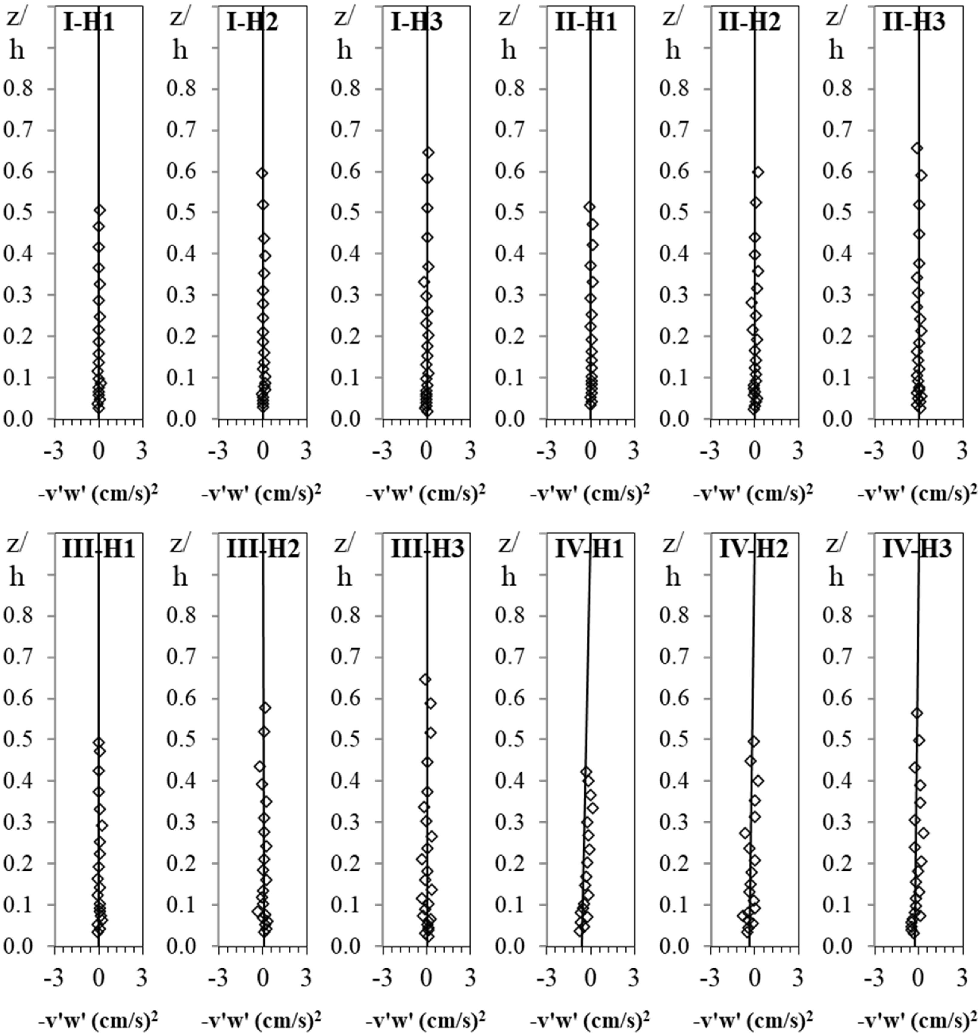
Turbulent stresses or Reynold stresses for an incompressible flow include Reynolds shear stresses (τxz = −ρu′w′, τxy = −ρu′v′, and τyz = −ρv′w′) and Reynolds normal stresses (σx = −ρu′2, σy = −ρv′2, and σz = −ρw′2), where u′, v′, and w′ are the velocity fluctuations in the streamwise, spanwise, and vertical directions, respectively [5]. For simplification, the Reynolds stress is often divided by the mass density ρ with the dimension of [L2/T2]. These terms are called either the second moments or second-order correlations which are not never zero. They are used to describe characteristics of turbulent flow in the Cartesian coordinate system, which are investigated in this study to estimate bed shear stress, along with TKE.
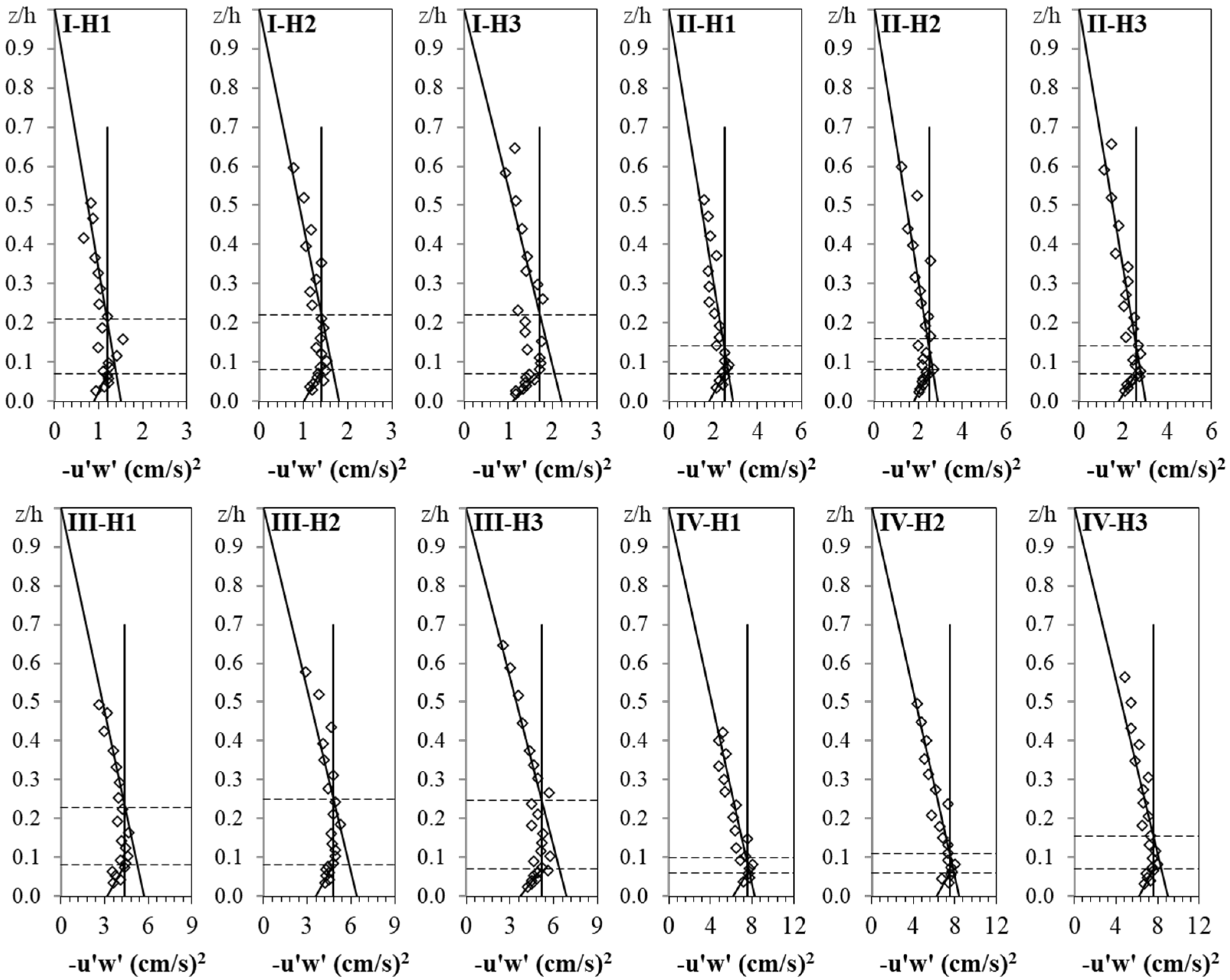
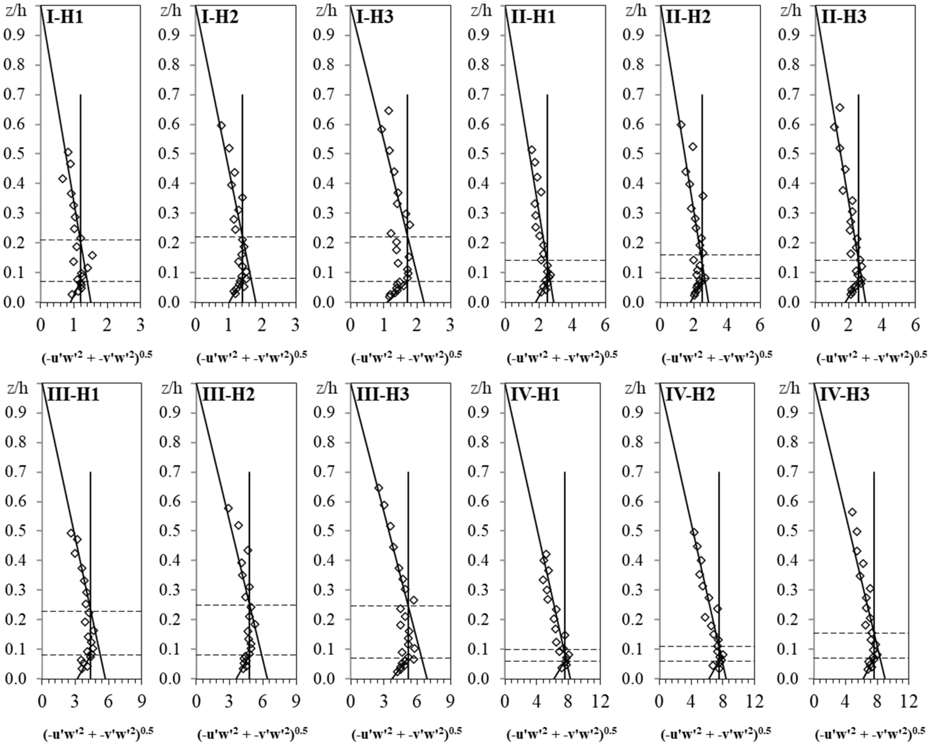
Extending the linear portion of the vertical distribution of −u′w′ (above the damping zone near the bed) towards the bed is one of the most reliable approaches to estimate bed shear stress in steady-uniform flows [5,8,9,10]. This approach is also called the direct covariance method [7] and can be used effectively in presence of sediment movement [9] as efficiently as under the fixed bed condition. This method can be used to determine bed shear stress directly, but the access to advanced equipment with high frequency for acquiring velocity fluctuations is a major challenge in a natural river condition [11]. Sarkar and Dey [12] claimed that the damping zone of the −u′w′ profile is related to a reduction in the turbulence intensity in both streamwise and vertical directions in the zone near a channel bed. They argued that this phenomenon may be due to the effect of flow non-uniformity in the vicinity of the channel bed, which changes the linear distribution of −u′w′ in the zone near the bed. This damping zone is also reported by Dey et al. [13] under conditions of the incipient motion of sediment particles, and by Dey et al. [8] under conditions of bed load movement, both at a higher distance from the bed compared to the immobile bed conditions. Dey et al. [8] reported that, in the presence of sediment transport, the vertical distribution of Reynolds shear stress over the entire flow depth showed a reduction. It was claimed that the reason for this reduction is related to the extra momentum that the main flow provides to maintain the motion of sediment particles and overcome the bed resistance. Additionally, the excessive damping of Reynolds shear stress near the bed, in mobile bed, can be related to decrease in the velocity fluctuations as a result of the reduction of the difference between the flow velocity and the movement speed of the sand particles [8]. Cossu and Wells [14] pointed out that the maximum value in the Reynolds shear stress verticals occurs at a point inside of the boundary layer where the velocity gradient is the maximum, but below this zone, the Reynolds shear stress decreases, and the viscous stresses increases.
It should be noted that in the presence of vegetation patches in the channel bed, the vertical distribution profile of Reynolds shear stress changes [15], and the method of the linear extension of the profile towards the channel bed is not practical. In non-uniform flows, Afzalimehr [16] and Emadzadeh et al. [17] took attention to the distribution of −u′w′ at the depth below the damping zone and derived a non-linear regression line across the entire water depth to estimate the bed shear stress. In general, the approach by means of −u′w′ is not only sensitive to the possible misalignment of the ADV probe from the flow streamwise direction but also affected by the non-uniformity of the flows [2,18,19]. It can also be affected by the presence of secondary currents [7]. To solve these problems, especially in oceanography, some researchers applied vector addition of −u′w′ and −v′w′ equal to (u′w′2 + v′w′2)0.5, to estimate the bed shear stress [14,20,21,22]. This approach can be especially useful in the field study of rivers and seas, where correct aligning the ADV probe with the flow streamwise direction is prone to error. However, the necessity of applying this approach in laboratory conditions needs to be investigated, especially when the flow is uniform, the secondary current is negligible and the ADV probe is well-aligned with the flow streamwise direction.
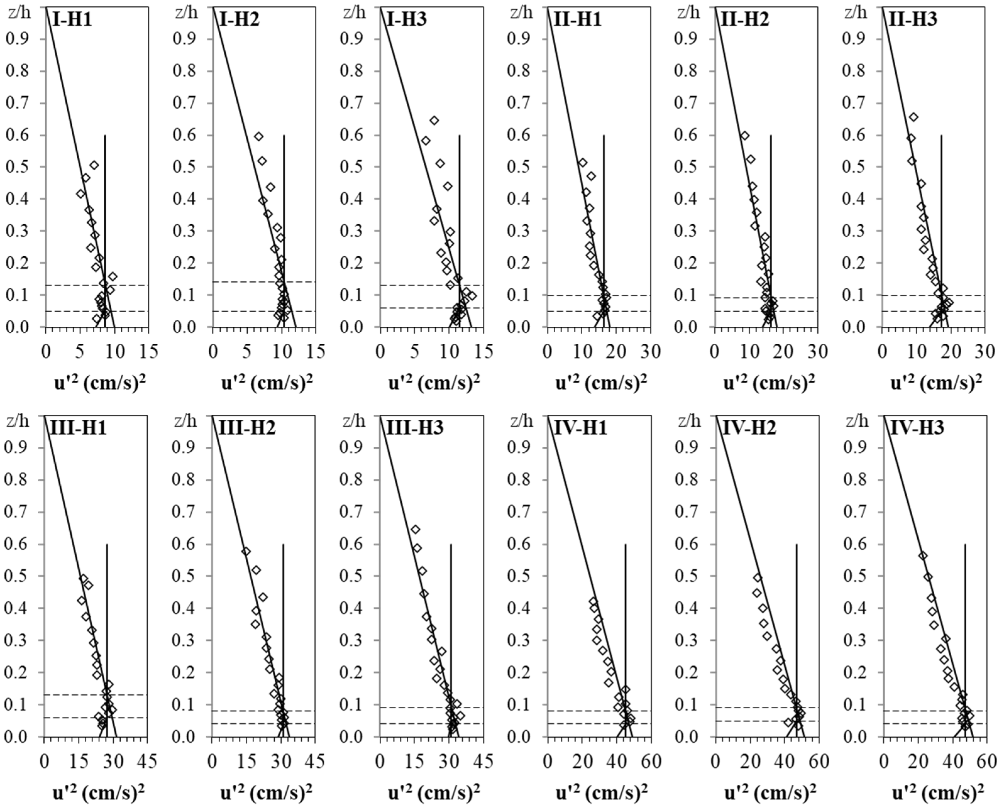
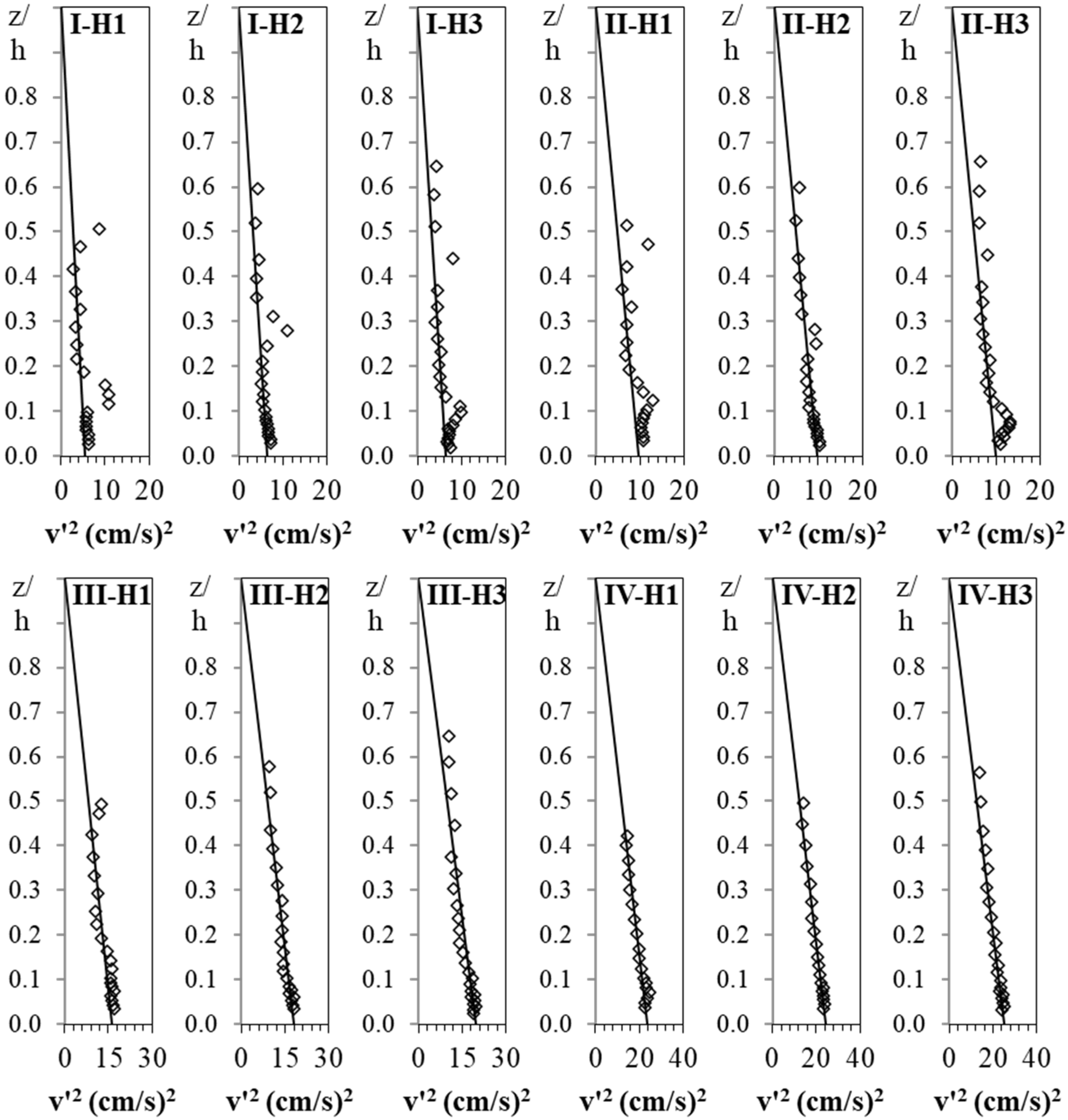
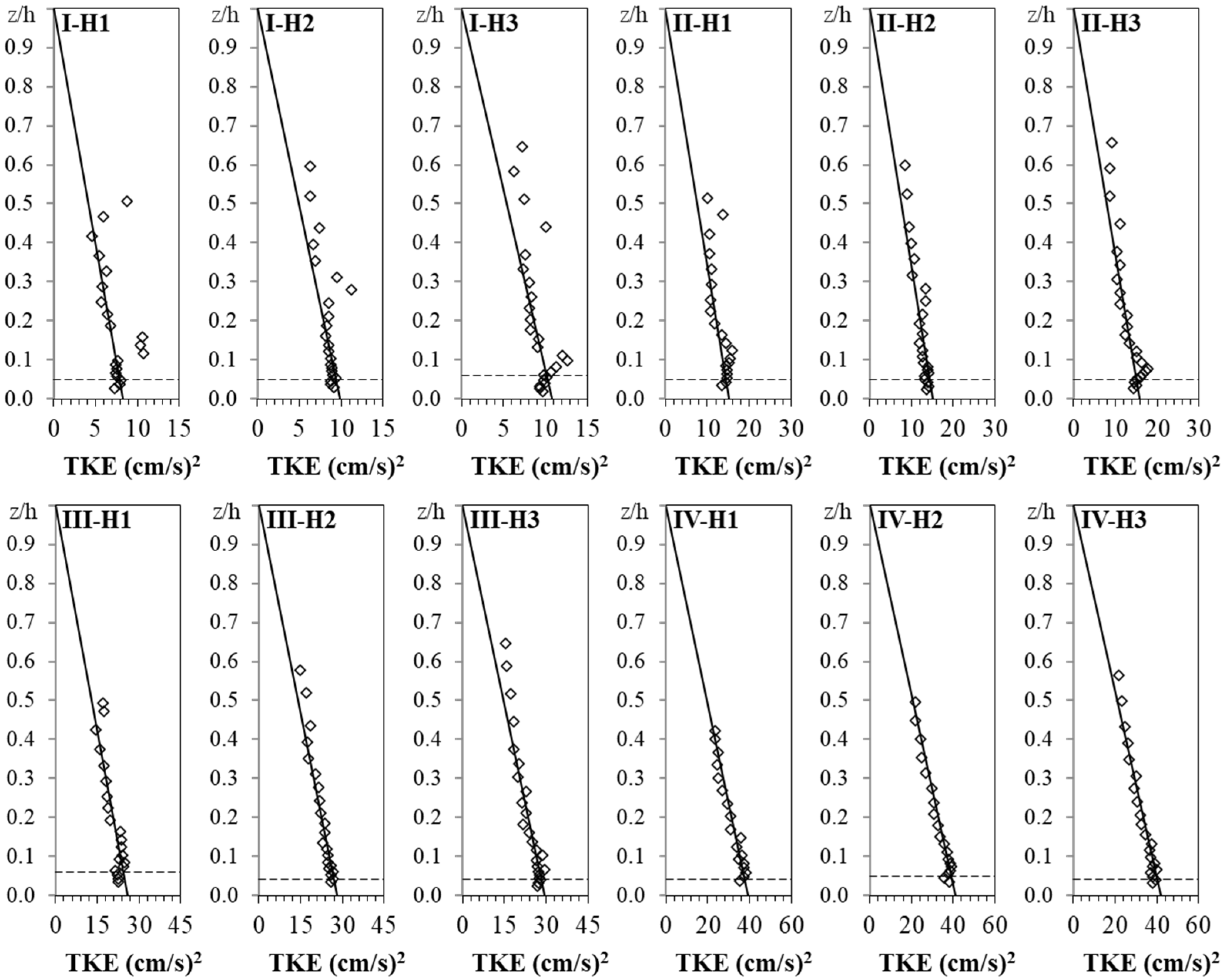
The turbulent kinetic energy TKE is the result of the absolute intensity of velocity fluctuations from the mean velocity in a cartesian coordinate system [23] and is equal to the sum of u′2, v′2, and w′2 divided by 2 multiplied by the mass density of water. Some researchers claimed that TKE is proportional to the bed shear stress with a simple linear relationship which can be used to determine the bed shear stress [7,19]. Obviously, applying all three components of the u′2, v′2, and w′2 in three directions [18], makes the TKE approach less sensitive to the misalignment of the ADV probe from the correct flow streamwise direction [19]. To estimate the bed shear stress, TKE should be multiplied by a specified coefficient of 0.19 [19,21,23,24,25,26,27], or 0.20 [28,29] or 0.21 [7], generally related to oceanography studies. Kim et al. [7] claimed that the TKE method is the most reliable approach, but more research work is required in the case of the coefficient that relates TKE to bed shear stress. This approach is widely accepted in oceanography studies, but surprisingly was rarely used in fluvial studies [2,26]. Biron et al. [2] successfully used this method with a coefficient of 0.19 in river studies. Pope et al. [23] claimed that the TKE approach could be used effectively in situations such as the presence of vegetation patches and bedforms in river beds where the application of some other well-known methods is almost impossible.
Voulgaris and Trowbridge [30] revealed that an ADV can acquire w′2 more accurately than u′2 and claimed that u′2 is more affected by noise errors. In this way, Kim et al. [7] tried to modify the TKE method and proposed that w′20 could be multiplied by a coefficient of 0.9 to estimate the bed shear stress. Results of experimental studies by Zhang et al. [26] showed that the w′2 method for measuring bed shear stress in rivers could be more handful than the TKE method, but the value of the coefficient needs to be modified. However, it seems that this approach needs to be further studied for clarifying to what extent the estimation of the bed shear stress can only rely on w′2.
Some researchers indicated that the above-mentioned methods for determining bed shear stress by means of −u′w′, TKE, and w′2 can be applied using the one-point measurement approach, especially in oceanography [2,7,23,31]. Biron et al. [2] and Pope et al. [23] satisfactorily applied the one-point measurement approach to estimate the bed shear stress by using both −u′w′ and TKE, respectively. Kim et al. [7] reported that the one-point measurement approach for determining the bed shear stress by using −u′w′ was a reliable method under a tidal condition. They recommended that the ADV sampling volume should be sufficiently close to the bed, located inside the constant shear stress layer. They also suggested that the ADV sampling volume should be at certain distance from the bed to avoid the influence of the bed materials on the sampling volume. Rashid [31] argued that the depth for the one-point measurement approach should be as close as possible to the bed, and thus recommended a depth of 4 mm above the sand bed for the one-point measurement method to estimate the bed shear stress using −u′w′, TKE, and w′2.
Despite the important role of the bed shear stress in studies of fluvial hydraulics, there is a lack of knowledge regarding the performance of different methods based on turbulence characteristics, especially under the critical condition of transitional flow over a sandy bed. The methods based on both TKE and w′2 are well-known methods used by oceanographers but have not received enough attention in river studies by river engineers. It is necessary to examine the applicability of these approaches in river studies and determine the appropriate coefficients in order to estimate the bed shear stress, especially under the conditions mentioned above. Additionally, the possibility of using other Reynolds normal stresses including u′2 and v′2 to estimate the bed shear stress should be examined. The necessity of the approach of the vector addition of −u′w′ and −v′w′ for different conditions in the laboratory needs to be investigated. By analyzing and simplifying all vertical distribution of Reynolds shear and normal stresses as well as TKE, the main purpose of this study is to investigate all possible ways for estimating bed shear stress under the mentioned specific conditions and answer some questions such as: is it sufficient to estimate bed shear stress by multiplying the values of Reynolds normal shear stresses including u′2, v′2, and w′2 as well as TKE at the bed by a specified constant coefficient? Are the determined coefficients dependent on the values of shear Reynolds number within the range of transitional flow conditions?

2. Materials and Methods

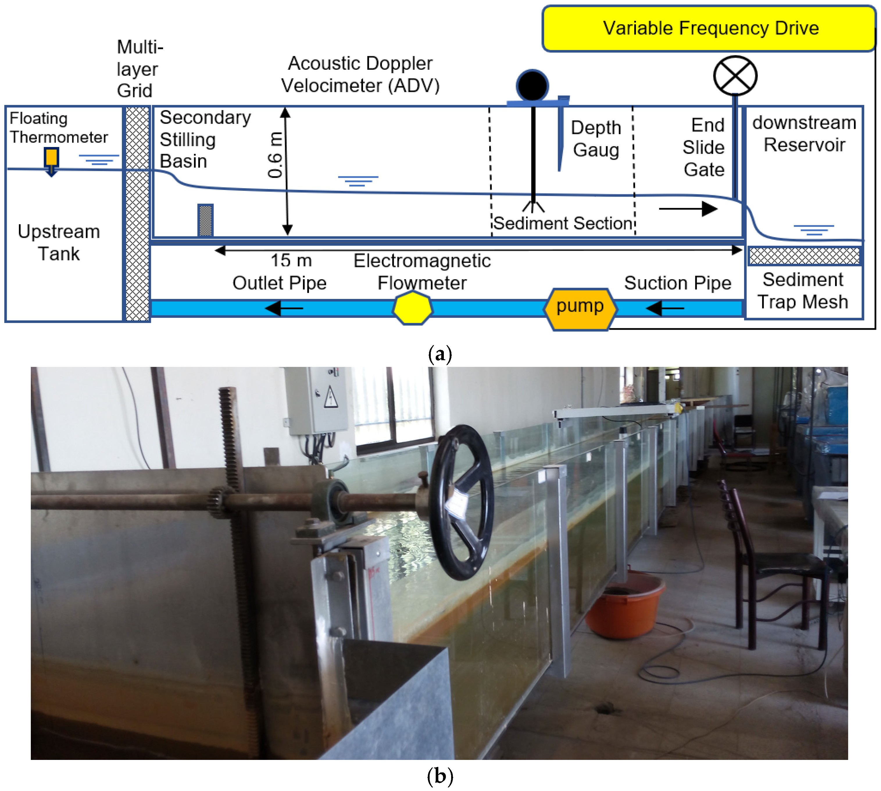
A rectangular long and wide flume was used for doing experiments (
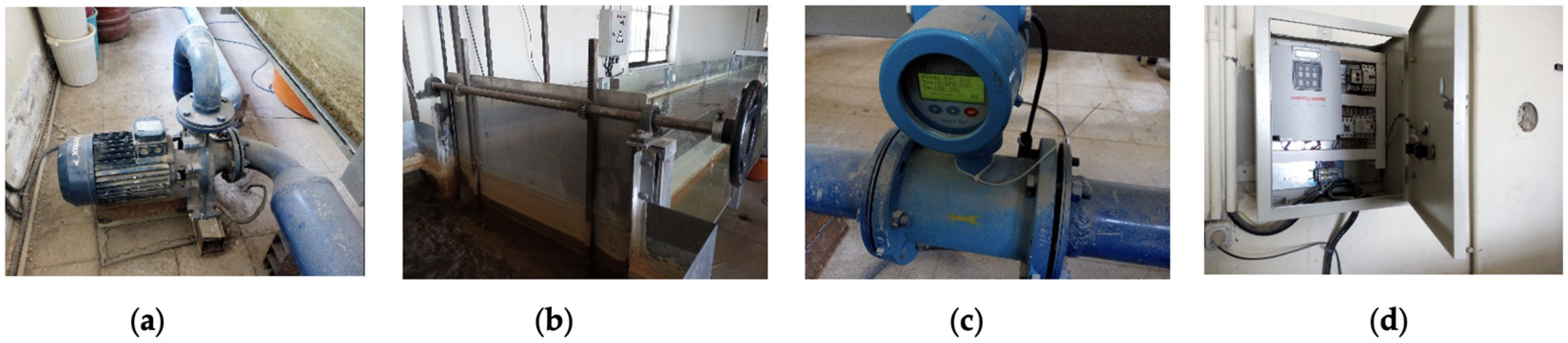
Figure 1). The flume is 15 m long, 0.6 m deep, and 0.9 m wide. This wide and long flume enables the flow to achieve a fully developed flow with a minimal side-walls effect. The flume side walls are transparent to facilitate observations of the movement of sediment particles during each experimental run. Water was recirculated between the upstream storage tank and the downstream reservoir using a pipeline with a centrifugal pump (Figure 2a) with a discharge capacity of 50 lit/s. Water was spilled over a slide-gate located at the end of the flume (Figure 2b) into a downstream reservoir (equipped with a sediment trap mesh). The water temperature was continuously recorded using a floating electrical thermometer located in the upstream water tank. In order to reduce the flow oscillations and dissipate additional disturbances, a multi-layer grid was placed in the upstream tank and a secondary stilling basin at the flume entrance. The flow discharge was measured using a high-precision electromagnetic flowmeter (Figure 2c) with a maximum relative percentage error of 0.5%, installed on the pump outlet pipe. The flow rate was regulated by adjusting the frequency rate applied to the pump electromotor, using a variable frequency drive (Figure 2d). A simple depth point gauge with a resolution of 0.5 mm was used to measure the water depth during each experimental run.
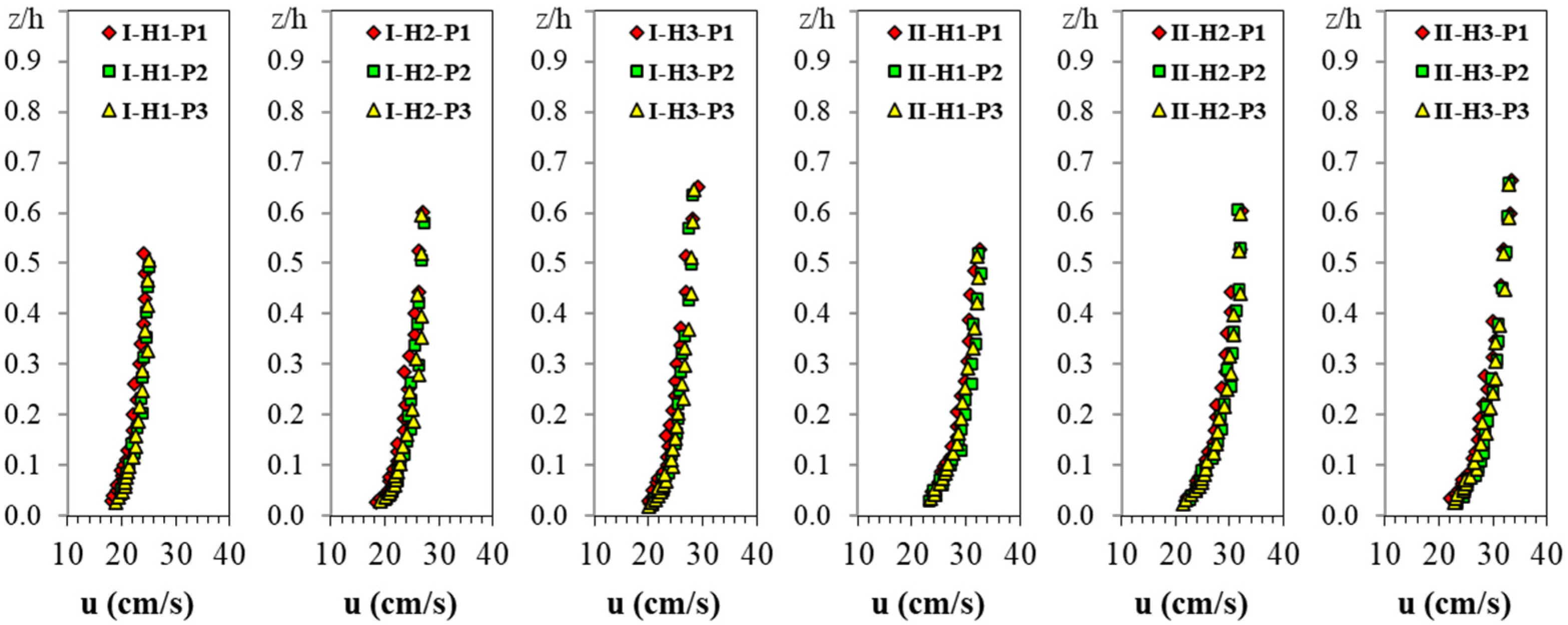
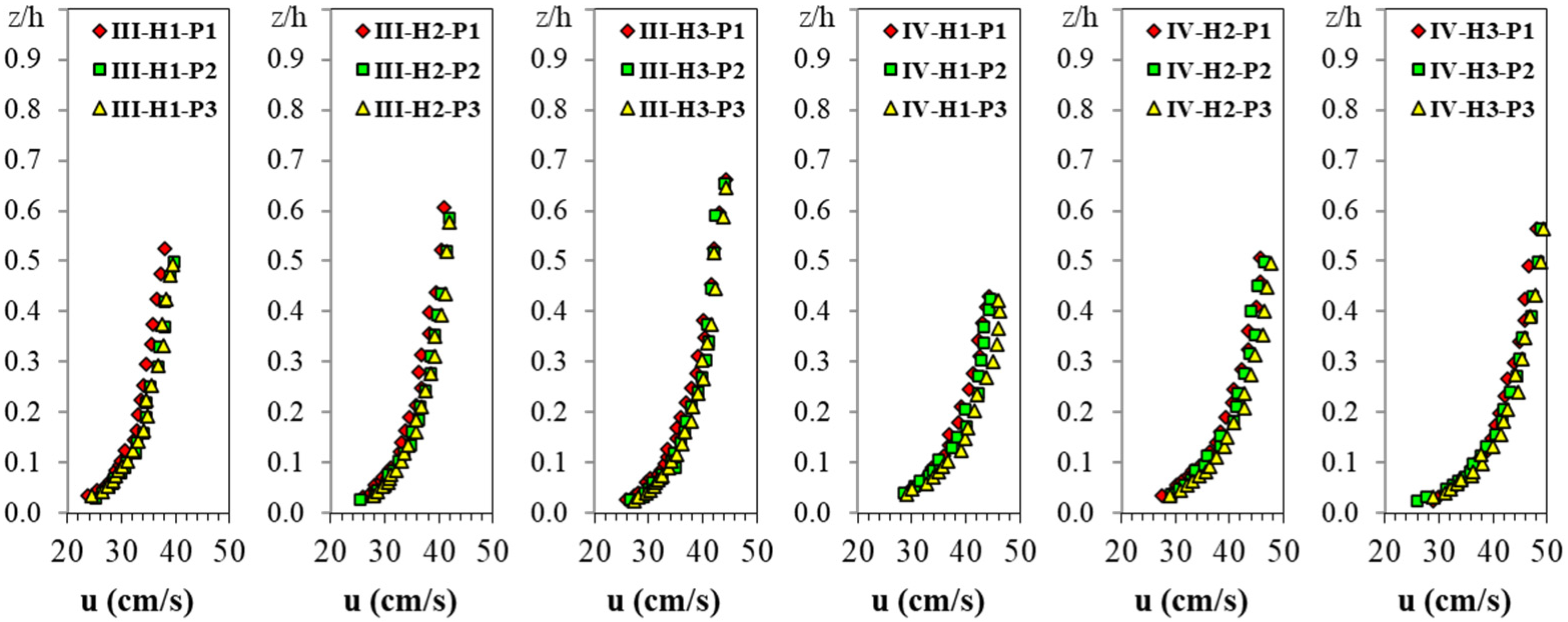
An acoustic doppler velocimeter (ADV) including a four-beam down-looking probe was applied to record velocity fluctuations in three directions in a cartesian coordinate system including the streamwise u (to the downstream), spanwise v (to the left side), and vertical w (from the bed towards the water surface) directions. All measurements of flow velocities were taken under conditions of incipient motion of sediment particles in the sandy bed. According to the ADV user instructions available at www.nortek-as.com, accessed on 26 October 2015, the ADV acoustic frequency was 10 MHz able up to 200 Hz sampling frequency made by the Nortek Corporation with a maximum relative percentage error equal to 0.5%. The last version (version 1.22) of Nortek’s specific interface software named Vectrino Plus was used to collect data. At each point, the ADV measurement lasted 2 min for collecting 24,000 data. The first point for velocity measurement should be at least 60 mm below the water surface considering the approximate distance of 50 mm between the ADV transducer and focal point of the sampling volume, together with a required probe-head submergence of at least 10 mm underwater to avoid bubble exposure. On the other hand, to avoid interference of the sampling volume with the channel bed, it was inevitable to ignore data collection at a distance of 3–4 mm to the bed. Therefore, because of the inherent limitation of the ADV device, data sampling along each profile was limited to a range of 3–4 mm above the bed to 60 mm below the water surface.
Because data collected using an ADV can be affected by the doppler signal noise [32], the data should be refined using software called WinADV32 (version 2.024, Water Resources Research Laboratory, U.S. Bureau of Reclamation, Denver, Colorado, downloaded from http://www.usbr.gov/wrrl). In this case, a filter called the phase–space threshold despiking developed by Goring and Nikora [32] and modified by Wahl [33] was applied. Additionally, the minimum acceptable correlation coefficient and signal-to-noise ratio were determined equal to 70 and 15, respectively. Finally, after removing about 18% of the damaged sample data, the profiles for flow velocity, TKE, and Reynolds normal and shear stresses were obtained. In this way, by using the “Data Conversion” command and selecting the NDV option in the Vectrino Plus software (version 1.22, Nortek AS, Vangkroken 2, NO-1351 RUD, Norway, downloaded from www.nortek-as.com), the extension of the files acquired by ADV was converted from “vno” to the “adv” in order to be available for the WinADV32. Then, in the WinADV32 software, after determining the desired filters by running the “Process Many” commands, the summary statistics of the filtered data were computed for all points of a profile and merged into a file with the extension of “sum”. This file could be opened in the MS-Excel software to draw the vertical distribution of velocity and turbulence characteristics.
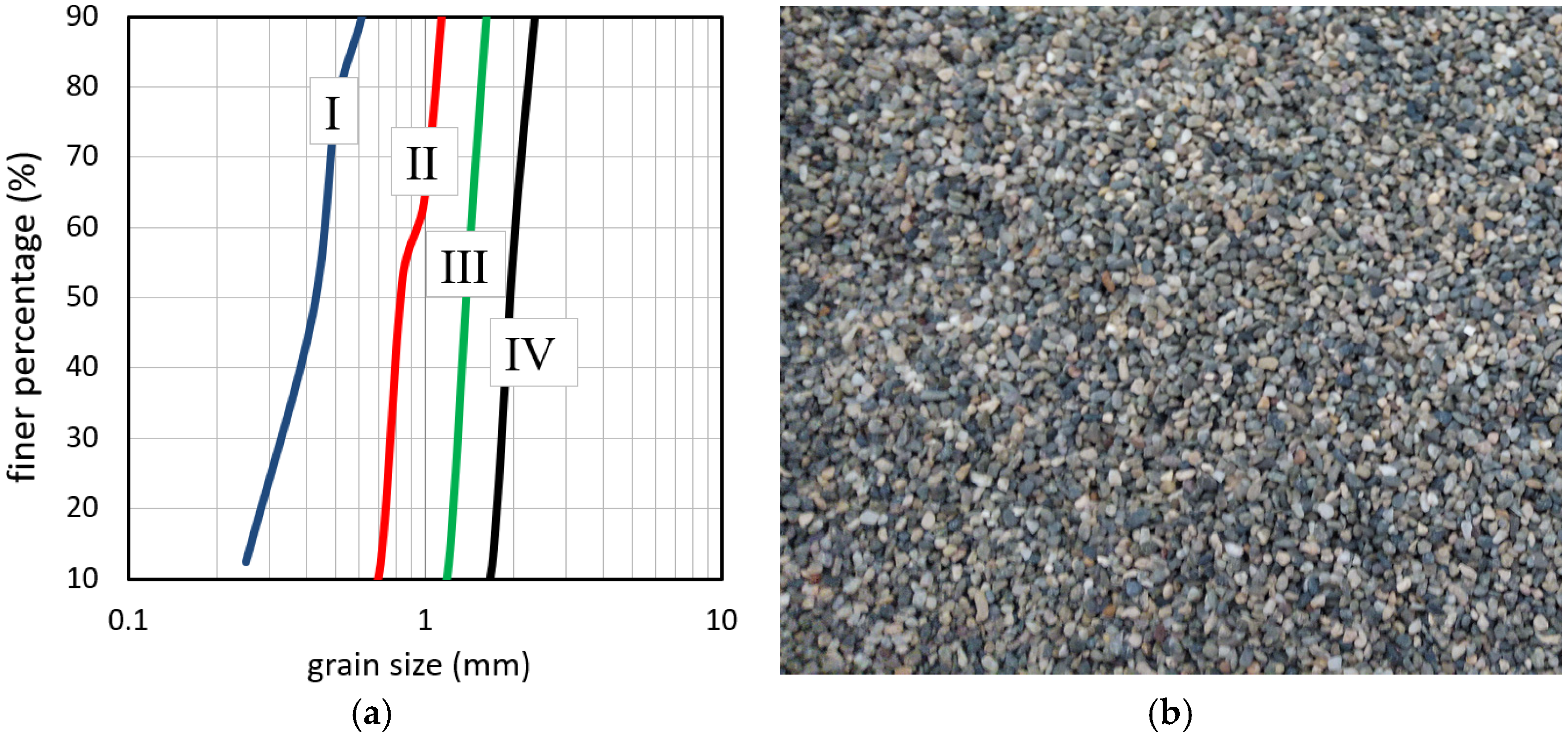
Four groups of uniform sand particles numbered I, II, III, and IV with median grain sizes of 0.43, 0.83, 1.38, and 1.94 mm, with a mass density of 2.65 g/cm3 were used in this experimental study. The median grain size of all four groups is less than 2 mm in the range of sand grain size [34]. According to the well-known grain size classification [5], group “I” was classified as medium sand, group II as coarse sand, and both groups III and IV as very coarse sand. The geometric standard deviation of particle size distribution is between 1.16 to 1.45, indicating an acceptable uniform distribution of sediment particles. The grain size distribution curves of four sediment groups were presented in Figure 3a together with a picture of a sample of sediment used in this experiment (Figure 3b). Three flow depths H1, H2, and H3 equal to 100, 120, and 140 mm, respectively, were used for experiments using sediment groups “I”, “II”, and “III”. For sediment group “IV”, three flow depths of 91, 104, and 120 mm, respectively, were used. The bed of a flume section which is 4 m long was covered with a sand layer with a thickness of 3 cm. It should be noticed that this homogeneous sandy bed is different from the real situation in natural rivers, but this assumption is necessary for this study to evaluate the flow characteristics under the condition of incipient motion of different sizes of sediment particles. The flume section between this sand bed and flume entrance was 8 m long and can provide suitable conditions for a fully developed flow. To reduce the effect of the end slide-gate, the flume section with the sand bed was located 3 m upstream from the end slide-gate of the flume. The flume bed of both the upstream and downstream sections from the sand bed section was covered with coarse material that was unable to move during the experiments.
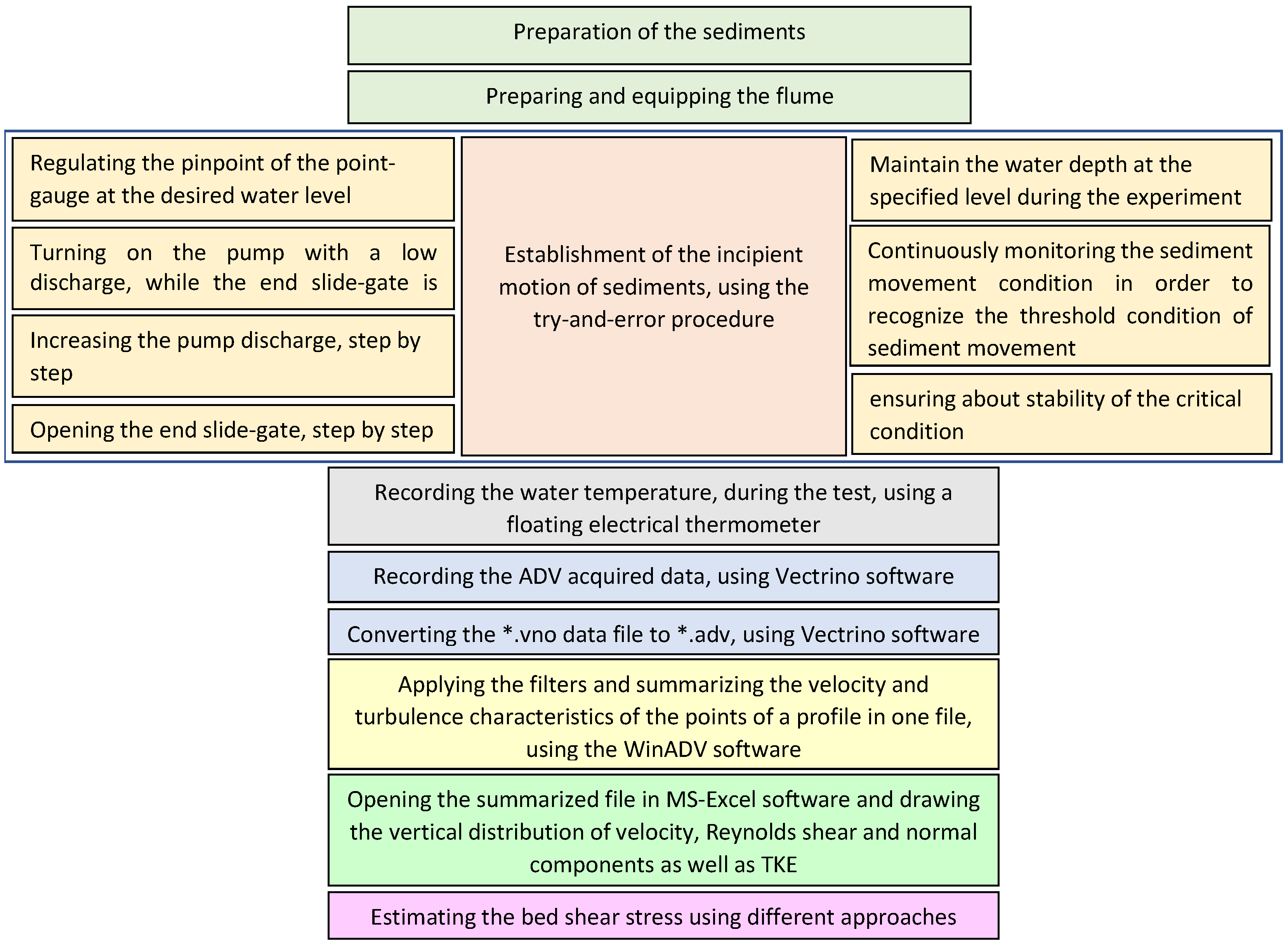
The medium transport of the Kramer visual observation method was considered as the criterion for determining the threshold condition which indicated the movement of a large number of particles with median grain size, without changing the bed-surface configuration [9]. By changing the pump discharge and adjusting the end slide-gate at the end of the flume, the specified flow velocity can be created at the desired water depth. Firstly, the pinpoint of the point gauge was fixed at the level of desired water surface. To prevent sediment particles from washing away, the pump was turned on with a low flow rate of about 5 lit/s, using the variable frequency drive, while the end slide-gate was closed. Once touching the pre-regulated pinpoint of the point gauge with water, by slightly opening of the end slide-gate a uniform low-velocity flow was established at the desired water depth. To increase the flow velocity to achieve the incipient motion of bed materials at the pre-determined water depth, using the try-and-error procedure, the pump discharge and the opening of the end slide-gate were increased gradually. This time-consuming procedure continued until achieving the threshold condition. It should be noted that the mobility of sediment particles was monitored for about 10 min to ensure about stability of the critical condition. The experimental process for all experiments was summarized in Figure 4.

3. Results and Discussion

3.1. Characteristics of Flow over the Sand Bed

To investigate the flow development along the flume section with the sand bed, three vertical lines for velocity measurements named P1, P2, and P3 were set up at the distance of 1, 2, and 3 m, respectively, from the upstream edge of the sand bed (or 9, 10 and 11 m from the flume entrance, respectively). As shown in Figure 5, the velocity profiles along these vertical lines (termed “velocity vertical”) had a similar pattern along the sand bed reach, indicating that a fully developed flow was formed along this section. The location of “P3” was selected to determine bed shear stresses for 12 different experiments under conditions of different flow depths and different sizes of sand particles. Note, the ADV was located in this location at a distance of 11 m from the flume entrance section or 4 m from the end slide-gate of the flume.
As reported, the closer to the side walls of the flume, the more obvious the dip phenomenon. Additionally, the effect of secondary currents along the center line of the channel is minimal [35]. Thus, all measurements were taken along the center line of the flume at a distance of 45 cm from the side walls. For flows with a sufficiently large aspect ratio (ratio of the flume width B to the flow depth h), B/h > 5, it is expected that the maximum velocity occurs at the water surface in both uniform and non-uniform flows [36,37] while it is reasonably free from the effect of side walls [38]. Considering the values of the aspect ratios in Table 1 (between 6.4 and 9.9) and the placement of the ADV in the center line of the flume in this experimental study, it was expected that all velocity verticals were free from the effect of the side walls and the maximum velocity occurred at the water surface. According to Table 1, the relative roughness of sediment particles at different water depths is very small and ranges from 0.003 to 0.021, indicating that the flow depth is much deeper compared to the grain size of sediment particles. The average water temperature was 20 °C, varied from 15 °C to 24 °C. Accordingly, the mean value of the kinematic viscosity coefficient ranged from 0.009 to 0.011 (with an average of 0.010) indicating no considerable changes. In the present study, the flow in all experimental runs was turbulent and subcritical flow. As shown in Table 1, the shear Reynolds numbers Re* obtained from this experimental study varied from 5 to 61, within the range of hydraulically transitional flow conditions [5]. To calculate the shear Reynolds numbers, the shear velocities were calculated using the estimated bed shear stresses obtained by the −u′w′ method and Nikuradse’s equivalent roughness (Ks) which is assumed to equal to the median size of sediment particles.
The viscous sublayer is a very thin layer near the bed (0 < z ≤ 5 ν/u*) with only laminar flow inside the viscous sublayer. The viscous shear stress inside the viscous sublayer is predominant and equal to the bed shear stress [5]. As shown in Table 1, the distance of the upper boundary of this layer from the bed (5 ν/u*) is between 0.2 and 0.4 mm. The transition or buffer layer is also a thin layer upon the viscous sublayer (5 ν/u* < z < 30 ν/u*) that is affected by both water viscosity and flow turbulence. The upper boundary of this layer (30 ν/u*) is located at a distance of 0.9~2.6 mm from the bed. Obviously, with the increase in the bed shear stress, which is directly related to the flow velocity, the thickness of these layers was decreased. Due to the inherent limitation of an ADV at the near bed zone, it is unable to acquire data by using an ADV inside of these two layers. Therefore, all data measured using an ADV at the depth of z/h < 0.2 are related to the turbulent wall shear layer or logarithmic layer (30 ν/u* ≤ z < 0.2 h), where the law of the wall is valid, and the Reynolds shear stress is predominant. According to Table 1, a number of 10 to 14 measurement points are located inside this turbulent wall shear layer. It should be noted that the layer including the viscous sublayer, buffer layer, and turbulent wall shear layer is usually called the inner layer [5]. Inside of the turbulent outer layer (z ≥ 0.2 h), the variation of flow velocities along the vertical line decreases with the increase in the depth z/h. The turbulent outer layer can be divided into two zones including the intermediate layer (0.2 h ≤ z ≤ 0.6 h) and the free surface layer (0.6 h < z ≤ 1). As shown in Table 1, only three experimental runs (I-H3, II-H3, and III-H3) have a measuring point in the free surface layer. In conclusion, due to the inherent limitation of the ADV, the velocity measurement in the free surface layer of a shallow flow using an ADV with a downward-looking probe is not possible. Therefore, the velocity and turbulent characteristics in this region should be predicted by extending the distributions in the intermediate layer. The number of points for data collection in the intermediate layer for all experimental runs is between eight and nine.

3.2. Bed Shear Stress Estimation Using the −u′w′ Method

As shown in Figure 6, the vertical distribution of −u′w′ increases linearly from the water surface to a specified flow depth near the bed. After that flow depth, exists a damping zone, and then −u′w′ decreases towards the bed. This result is comparable to those of many other researchers [8,12,13,14]. For clarification and simplification, the vertical distribution of −u′w′ was divided into three distinct zones from the water surface to the bed, as follows:
  • Increasing zone: a linear increase in −u′w′ from the water surface to the damping zone.
  • Damping zone: a limited portion near the bed with relatively unchanged values of −u′w′.
  • Decreasing zone: a linear decrease in −u′w′ from the damping zone to the bed.
It should be noticed that a lot of care is needed for accurately determining the location of these zones and selecting the points for describing each zone, as well as fitting the regression lines. According to Table 2, by extending a linear regression line in the increasing zone with zero value at the water surface towards the bed, the bed shear stress −u′w′0 was determined. This method is the most reliable and well-known method for estimating bed shear stress for uniform flows [5,8,9,10], and was applied as the main method for comparing results to those using other methods which considered in this study. Given the approximately constant values of −u′w′ in the damping zone, it is highly recommended to select the depth of one-point measurement within this zone. As clearly shown in Table 2, the ratio of −u′w′0 to the values of −u′w′ in the damping zone −u′w′d are from 1.09 to 1.33 (with an average of 1.22). Therefore, it is recommended that the measured values using the one-point measurement method in the damping zone −u′w′d be multiplied by 1.22 to estimate the bed shear stress. This is in contrast to some reported studies [2] which assumed the value obtained by the one-point measurement method could be used to represent the bed shear stress. For confirmation, by multiplying the values in the damping zone by 1.22, the ratio of the results to −u′w′0 was obtained and ranged from 0.92 to 1.12 (standard deviation of 0.07), which indicates a good agreement.
In oceanography, the depth of the one-point measurement is considered at a relatively larger distance from the bed [7], but in shallow rivers, it must be placed at depths close to the bed [2]. It seems that the middle point of the damping zone could be recommended as the best location for the one-point measurement. Accordingly, this depth in Table 2 should be between z/h = 0.08 and z/h = 0.17 with an average depth of z/h = 0.13. This depth is comparable to the finding of Biron et al., [2] who showed that the maximum value of −u′w′ and TKE in river studies appear in the depth of z/h = 0.1. However, under a deeper water condition, this depth for the one-point measurement method can be different. This finding is different from some previous studies which suggested that the depth of the one-point measurement method should be as close to the bed as possible [31].
Some studies determined the −u′w′ distribution below the damping zone by extrapolating a non-linear regression line across the entire water depth, especially in non-uniform flows [16,17], and accordingly, the values of −u′w′0 in Table 2 were 1.32 to 2.00 (with an average of 1.66) times larger than the values obtained by extending a line towards the bed in the decreasing zone −u′w′b. This finding revealed that this approach for estimating the bed shear stress leads to a considerable underestimation and unreliable results.

3.3. Bed Shear Stress Estimation Using −u′v′ and −v′w′

Figure 7 shows the vertical distribution of −u′v′ for all experiments. Some data points are deviated from the profiles of the −u′v′ distribution, especially in experiments IV-H1, IV-H2, and IV-H3, and it is difficult to extend a line between those points. However, by extending a line from zero value at the water surface towards the bed, the values of −u′v′0 were obtained and presented in Table 3. Obviously, it is not possible to create a relationship between −u′w′0 and −u′v′0 and estimate the bed shear stress.
According to Figure 8, by extending a line from the point with zero value of −v′w′ at the water surface towards the bed, the values of −v′w′0 were determined. As shown in Table 4, for the first nine experiments, the values of −v′w′0 are very close to zero. However, the values for the last three experiments are −0.6, −0.4, and −0.3, respectively. The reason for such large absolute values of −v′w′0 for these three experiments seem to be related to a probable slight misalignment of the ADV probe from the downstream direction. Similar to the −u′v′ distribution, there is no relationships between the values of −u′w′0 and −v′w′0, indicating that it is not possible to estimate the bed shear stress using −v′w′0 values.

3.4. Bed Shear Stress Estimation Using the Vector Addition of −u′w′ and −v′w′

According to some studies [2,18,19], the vector addition of −u′w′ and −v′w′ was applied to reduce the −u′w′ sensitivity to the misalignment of the ADV probe from the streamwise direction. According to Figure 9, comparing to the values of −u′w′, the values of −v′w′ are so small and negligible. Thus, the vertical distribution of the vector addition of these terms (−u′w′2 + −v′w′2)0.5 and the vertical distribution of −u′w′ are nearly similar. As shown in Table 5, the values of vector addition of −u′w′ and −v′w′ at the bed [(−u′w′2 + −v′w′2)0.5]0, obtained by extending a line in the increasing zone, are equal to −u′w′0 values, implying that the estimation of the bed shear stress using −u′w′ method is not obviously affected by some not-considerable misalignments of the ADV probe in laboratory, where the experimental conditions are well controlled. However, an obvious misalignment of the ADV probe in a natural river happens very likely. Thus, the application of the vector addition of −u′w′ and −v′w′ can be more recommended.

3.5. Bed Shear Stress Estimation Using u′2

It should be noted that the turbulence intensity, expressed as the root mean square (RMS), is the square root of Reynolds normal stress (divided by -ρ) [5]. Therefore, the methods based on Reynolds normal stresses can be considered as a kind of turbulence intensity approach. As shown in Figure 10, the vertical distribution of u′2 has the similar distribution pattern to that of −u′w′, including a linear increase from the zero value of u′2 at the water surface to a damping zone and then a decrease towards the bed. Therefore, the vertical distribution of u′2 similar to −u′w′ verticals were simplified into three zones, including the increasing, damping, and decreasing zones. In comparison, the height of the damping zone for the u′2 distribution is less than that of −u′w′ verticals, and the decreasing zone is less recognizable. However, the decreasing zone is clearly visible in verticals for following eight experimental runs: I-H2, I-H3, II-H1, II-H2, II-H3, III-H1, III-H2 and III-H3.
The values of u′2 at the bed u′20 were determined by extending a line in the increasing zone to the bed and was presented in Table 6. The ratio of −u′w′0 to u′20 is between 0.15 and 0.20 (with an average of 0.17). In this case, by multiplying u′20 by 0.17, the ratio of the calculated results (0.17 u′20) to −u′w′0 was obtained between 0.84 and 1.13 (with a standard deviation of 0.09), which indicated that the values of u′20 can be used to predict the bed shear stress multiplying by 0.17. Those 12 experiments were divided into two groups, namely, group A includes experiments related to sediment groups I and II with a range of shear Reynolds number between 5 to 14, and the group B includes experiments related to sediment groups III and IV with a range of shear Reynolds number between 34 and 61. The threshold velocity for the incipient motion of bed materials for groups A and B are between 23.6 and 30.6, and between 36.9 and 45.7 cm/s, respectively. One can see from Table 6, the ratio of −u′w′0 to u′20 for group A varies from 0.15 to 0.17 (with an average of 0.16), and for group B is between 0.16 and 0.20 (with an average of 0.18). By multiplying u′20 values of groups A by 0.16, and u′20 values of group B by 0.18, respectively, the ratio of the calculated results (0.16u′20 for group A, and 0.18u′20 for group B) to −u′w′0 for group A was between 0.97 and 1.07 (with a standard deviation of 0.04), and for group B was between 0.89 and 1.10 (with a standard deviation of 0.07). These values indicate that for a flow under a transitional flow condition, the relationship between u′20 and −u′w′0 can be slightly affected by the shear Reynolds number. However, it is feasible for estimating the bed shear stress for the entire range of shear Reynolds number by multiplying the value of u′20 by 0.17.
According to Table 6, the average depth of the lower and upper limitation of the damping zone are equal to z/h = 0.05 and z/h = 0.10, respectively. The ratio of u′20 to the values of in the damping zone u′2d is between 1.08 and 1.17 (with an average of 1.12). By multiplying u′2d values by 1.12, the ratio of the calculated results (1.12u′2d) to −u′20 was obtained between 0.96 and 1.04 (a standard deviation of 0.07), which indicates that the value of u′20 could be effectively estimated with the one-point measurement method in the appropriate depth of damping zone (with an average of z/h = 0.08).

3.6. Bed Shear Stress Estimation Using v′2

As shown in Figure 11, for bed material using both sediment groups I and II, some data points deviated from the profiles of vertical distribution of v′2 (note: v′ is the velocity fluctuations in the spanwise direction), which may be related to some unexpected doppler noises. Despite this problem, the values of v′2 decrease linearly towards the bed without any detectable turning point or decreasing zone. By extending a line from zero value at the water surface towards the bed, the values of v′2 at the bed (v′20) were determined, as shown in Table 7. The ratio of −u′w′0 to v′20 is between 0.28 and 0.36 (with an average of 0.33). We multiplied, the values of v′20 by 0.33, and the ratio of the results (0.33v′20) to −u′w′0 was obtained with a range from 0.92 to 1.19 (with a standard deviation of 0.09). This result indicates that it is possible to estimate the bed shear stress by means of the values of v′20. Results showed that the coefficient for group A is between 0.28 and 0.34 (with an average of 0.30), and for group B is between 0.34 and 0.36 (with an average of 0.35). For sand group A, the v′20 values are multiplied by 0.30, and for sand group B, the v′20 values are multiplied by 0.35. Then, the ratio of results (0.30v′20) to −u′w′0 for group A was between 0.89 and 1.08 (with a standard deviation of 0.06), and the ratio of results (0.35v′20) to −u′w′0 for group B was between 0.97 and 1.02 (with a standard deviation of 0.02). These values indicate that the range of the shear Reynolds number could somehow influence the relationship between v′20 and −u′w′0. In the case of the estimation of v′20 using the one-point measurement method, due to the presence of scattered points in the verticals, there is a risk that the measured single data may be invalid. Anyway, given the linear distribution from the zero value of v′2 at the water surface to the bed, the value of v′20 could be estimated to be equal to the one-point measured value divided by the difference between one and the relative depth of the point.

3.7. Estimation of Bed Shear Stress Using w′2

The vertical distribution profiles of w′2 for all experiments are shown in Figure 12 (note: w′ is the velocity fluctuations in the vertical direction). Obviously, the values of w′2 in the main flow are almost constant and starts to decrease at a specific depth near the bed without any recognizable damping zone that is comparable to the finding of Grass [38]. Grass showed that the values of w′2 in the main flow are almost constant above a depth of about z/h = 0.1 near the bed, albeit with a slightly increase, and then decrease to the bed for all smooth, transitional and rough flows. However, in this study, the vertical distribution of w′2 was simplified into two distinct zones, as below:
  • Unchanged zone: unchanged w′2 values from the water surface to a specified depth near the bed where w′2 starts to decrease.
  • Decreasing zone: a linear decrease in w′2 values near the bed towards the bed.
By extending a vertical line between the points in unchanged zone to the bed, the values of w′2 at the bed w′20 were determined. According to Table 8, the ratio of −u′w′0 to w′20 is varied from 1.06 to 1.43 (with an average of 1.24). This average ratio differs significantly from the ratio of 0.9 proposed by Kim et al. [7] for the tidal deep-water condition. This result of the present study confirms the recommendation of Zhang et al. [26] regarding the modification the coefficient proposed by Kim et al. [7], especially in river studies. The values of w′20 were multiplied by 1.24 and the ratios of 1.24w′20 to −u′w′0 were obtained and ranged from 0.87 to 1.17 (with a standard deviation of 0.10), which indicates that the bed shear stress can be estimated using the values of w′20. According to Table 8, the coefficient for group A is between 1.06 and 1.16 (with an average of 1.13), and for group B is between 1.28 and 1.43 (with an average of 1.36). For sand group A, the w′20 values are multiplied by 1.13, and for sand group B, the w′2 values are multiplied by 1.36. Then, the ratio of results (1.13 w′2) to −u′w′0 for group A was between 0.97 and 1.07 (with a standard deviation of 0.04), and the ratio of results (1.36 w′2) to −u′w′0 for group B was between 0.95 and 1.06 (with a standard deviation of 0.04). This finding indicates that the coefficient is proportional to the shear Reynolds number. These values show that although one unique coefficient of 1.24 applied for the entire range of the shear Reynolds number was sufficient, one can obtain better results (or closer values to −u′w′0) by applying two different coefficients for groups A and B, respectively.
Obviously, to estimate w′20 using the one-point measurement method, the measuring depth should be selected at the higher depth of the decreasing zone. In this case, it is important to determine the depth of the boundary between the unchanged and decreasing zones. According to Table 8, this depth is between z/h = 0.08 to 0.14 (with an average of 0.11), which is in good agreement with the result of Grass [38]. Therefore, the depth of the one-point measurement method should be averagely higher than z/h = 0.11.

3.8. Estimation of Bed Shear Stress Using TKE

Given that the value of TKE at each point is equal to the sum of u′2, v′2 and w′2 divided by 2, the pattern of the vertical distribution of TKE be developed based on all velocity fluctuation components of turbulent flow. As shown in Figure 13, the verticals of TKE are affected by the scattering of data observed in the vertical distribution of v′2 related to the particle size of bed material, namely, sediment groups I and II. Given that the u′2 possesses the largest portion of TKE values compared to v′2 and w′2, the vertical distribution of TKE is expected to have the similar pattern to that of u′2. However, due to the effects of v′2 and w′2, an obvious damping zone is not observed, and only a small decreasing zone is located near the bed. Thus, the TKE verticals include a decreasing and increasing zones with a turning point near the bed.
By extending a line through TKE points from the zero value at the water surface towards the bed in the increasing zone, the TKE values at the bed (TKE0) were determined. As shown in Table 9, in accordance with Soulsby [28,29], the ratio of −u′w′0 to TKE0 is varied from 0.18 to 0.23 (with an average of 0.20). The ratio of 0.2TKE0 to −u′w′0 was obtained, which varied from 0.85 to 1.11 (with a standard deviation of 0.08), indicating that TKE0 can be effectively used to estimate the bed shear stress. Additionally, since the TKE method applies all three components of Reynolds normal stresses in three directions [18], it is less sensitive to the probable misalignment of the ADV probe [19], it is more preferred compared to the u′2, v′2 and w′2 approach. According to Table 9, the ratio of −u′w′0 to TKE0 for sand group A is between 0.18 and 0.20 (with an average of 0.19) which is consistent with results of other researchers [19,21], and the ratio of −u′w′0 to TKE0 for sand group B is between 0.20 and 0.23 (with an average of 0.22) which is comparable with 0.21 proposed by Kim et al. [7]. For sand group A, the TKE values are multiplied by 0.19, and for sand group B, the TKE values are multiplied by 0.22, respectively. The ratio of results (0.19TKE) to −u′w′0 for group A was calculated between 0.93 and 1.05 (with a standard deviation of 0.04), and the ratio of results (0.22TKE) to −u′w′0 for group B was calculated between 0.94 and 1.07 (with a standard deviation of 0.05), indicating an improvement in the results. However, applying the unique coefficient of 0.2 is acceptable and can be recommended. According to Table 9, the depth of turning point between the increasing zone and the decreasing zone is varied from z/h = 0.04 to z/h = 0.06 (with an average of 0.05). For the one-point measurement approach, considering the risk of the influence from the invalid data points, the value of TKE0 could be estimated to equal to the one-point measured value divided by the difference between one and the relative depth of the point.
In Table 10, the ratio of all three components of the Reynolds normal stresses and TKE are presented. The values of u′20/TKE0, v′20/TKE0, and w′20/TKE0 are varied from 1.16 to 1.25 (with an average of 1.21), from 0.60 to 0.66 (with an average of 0.63) and from 0.15 to 0.18 (with an average of 0.16), respectively. These values indicate that the variation of the ratios in all experiments is considerably small. Additionally, the values of u′20, v′20, and w′20 are about 60.5%, 31.3%, and 8.2% of the values of (u′20 + v′20 + w′20), respectively. In this case, by knowing one of the values of u′20, v′20, w′20, or TKE0, the other terms can be estimated with acceptable accuracy.

4. Conclusions

Twelve experiments have been conducted to investigate the relationship between the turbulence characteristics and the bed shear stress under conditions of incipient motion of sand particles in the shallow transitional flows. The vertical distribution of −u′w′ showed a linearly increasing trend from the zero value at the water surface to the depth of z/h = 0.18; then followed by a damping zone with relatively unchanged −u′w′ at the depth of 0.07 < z/h < 0.18, and finally a decreasing zone with a decrease in −u′w′ towards the bed. By extending a regression line in the increasing zone, the value of the −u′w′0 was determined, which was considered as the bed shear stress and used to evaluate results using other methods. Results showed that, under such a laboratory condition with uniform flow and well-aligned ADV probe, the vector addition of the −u′w′ and −v′w′ is not necessary. The vertical distribution of u′2 has the same distribution profile as that of −u′w′, and can be simplified into three zones, but with a less height of the damping zone, and less recognizable the decreasing zone. The values of v′2 decreased linearly towards the bed without any detectable turning points. With respect of w′2, the values in the main flow were almost constant and started to decrease at the depth of z/h = 0.11 without any obvious damping zone. Along TKE verticals, a dominated increasing zone and a small decreasing zone were observed with a turning point near the bed at a depth of z/h = 0.05. The bed shear stress can be effectively estimated by multiplying the values of u′20, v′20, w′20, and TKE0 by 0.17, 0.33, 1.24, and 0.20, respectively. The estimated coefficient for TKE is in agreement with those in the literature. Since the TKE method applies all three components of Reynolds normal stresses in three directions, the TKE method seems to be preferred to comparing to the u′2, v′2, and w′2 methods. By classifying the laboratory experiments into two groups of A and B with a range of shear Reynolds number, respectively, from 5 to 14 and from 34 to 61, the bed shear stress for group A was estimated by multiplying the values of u′20, v′20, w′20, and TKE0 by 0.16, 0.30, 1.13, and 0.19, respectively, and for group B 0.18, 0.35, 1.36 and 0.22, respectively. This means under a transitional flow condition, to estimate −u′w′0, the coefficients for multiplying by u′20, v′20, w′20, and TKE0 are slightly increased from the hydraulically smooth to hydraulically rough flow conditions. For the one-point measurement approach, the middle point of the damping zone (at a depth of z/h = 0.13 for −u′w′ and z/h = 0.08 for u′2) was recommended to be used for estimating −u′w′0 and u′20 by multiplying the related values by 1.22 for −u′w′ and 1.12 for u′2, respectively. Given the linear distribution of v′2 and TKE from the zero value at the water surface to the bed, the value at the bed could be estimated which is equal to the one-point measured value divided by the difference between one and its relative depth at that point, considering z/h > 0.05 for TKE. In the case of w′2, it is recommended the depth for estimating w′20 using the one-point measurement approach should be selected in the unchanged zone with the depth of z/h > 0.11. It was estimated that the values of u′20, v′20, and w′20 are, respectively, about 60.5%, 31.3%, and 8.2% of their summation. The results of this study could be applied in such conditions similar to the current experiments. However, further studies should be carried out for other situations such as different particle sizes of bed material, bed load conditions, different water depths, and flow regimes.

Author Contributions

Conceptualization, R.S., H.A. and J.S.; methodology, R.S. and H.A.; software, R.S.; validation, R.S., H.A. and J.S.; formal analysis, R.S. and H.A.; investigation, R.S., H.A. and J.S.; resources, R.S., H.A. and J.S.; data curation, R.S.; writing—original draft preparation, R.S.; writing—review and editing, R.S., H.A. and J.S.; visualization, R.S.; supervision, H.A. and J.S.; project administration, H.A. and J.S. All authors have read and agreed to the published version of the manuscript.

Funding

This research received no external funding.

Data Availability Statement

The data used in this manuscript are available by writing to the first author.

Conflicts of Interest

The authors declare no conflict of interest.

References

  1. Bauer, B.O.; Sherman, D.J.; Wolcott, J.F. Sources of Uncertainty in Shear Stress and Roughness Length Estimates Derived from Velocity Profiles. Prof. Geogr. 1992, 44, 453–464. [Google Scholar] [CrossRef]
  2. Biron, P.M.; Robson, C.; Lapointe, M.F.; Gaskin, S.J. Comparing different methods of bed shear stress estimates in simple and complex flow fields. Earth Surf. Process. Landforms 2004, 29, 1403–1415. [Google Scholar] [CrossRef]
  3. Afzalimehr, H.; Anctil, F. Accelerating shear velocity in gravel-bed channels. Hydrol. Sci. J. 2000, 45, 113–124. [Google Scholar] [CrossRef]
  4. Wilcock, P.R. Estimating Local Bed Shear Stress from Velocity Observations. Water Resour. Res. 1996, 32, 3361–3366. [Google Scholar] [CrossRef]
  5. Dey, S. Fluvial Hydrodynamics; Springer: Berlin/Heidelberg, Germany, 2014. [Google Scholar] [CrossRef]
  6. Environmental and Water Resources Institute (U.S.); García, M.H. (Eds.) Sedimentation Engineering: Processes, Measurements, Modeling, and Practice; American Society of Civil Engineers: Reston, VA, USA, 2008. [Google Scholar] [CrossRef]
  7. Kim, S.-C.; Friedrichs, C.T.; Maa, J.P.-Y.; Wright, L.D. Estimating Bottom Stress in Tidal Boundary Layer from Acoustic Doppler Velocimeter Data. J. Hydraul. Eng. 2000, 126, 399–406. [Google Scholar] [CrossRef]
  8. Dey, S.; Das, R.; Gaudio, R.; Bose, S.K. Turbulence in mobile-bed streams. Acta Geophys. 2012, 60, 1547–1588. [Google Scholar] [CrossRef]
  9. Shahmohammadi, R.; Afzalimehr, H.; Sui, J. Assessment of Critical Shear Stress and Threshold Velocity in Shallow Flow with Sand Particles. Water 2021, 13, 994. [Google Scholar] [CrossRef]
  10. Vanoni, V.A.; American Society of Civil Engineers, and Environmental and Water Resources Institute (U.S.) (Eds.) Sedimentation Engineering, 2nd ed.; American Society of Civil Engineers: Reston, VA, USA, 2006. [Google Scholar] [CrossRef]
  11. Afzalimehr, H.; Rennie, C.D. Determination of bed shear stress in gravel-bed rivers using boundary-layer parameters. Hydrol. Sci. J. 2009, 54, 147–159. [Google Scholar] [CrossRef]
  12. Sarkar, S.; Dey, S. Double-averaging turbulence characteristics in flows over a gravel bed. J. Hydraul. Res. 2010, 48, 801–809. [Google Scholar] [CrossRef]
  13. Dey, S.; Sarkar, S.; Solari, L. Near-Bed Turbulence Characteristics at the Entrainment Threshold of Sediment Beds. J. Hydraul. Eng. 2011, 137, 945–958. [Google Scholar] [CrossRef]
  14. Cossu, R.; Wells, M.G. A comparison of the shear stress distribution in the bottom boundary layer of experimental density and turbidity currents. Eur. J. Mech.—B/Fluids 2012, 32, 70–79. [Google Scholar] [CrossRef]
  15. Shahmohammadi, R.; Afzalimehr, H.; Sui, J. Impacts of turbulent flow over a channel bed with a vegetation patch on the incipient motion of sediment. Can. J. Civ. Eng. 2018, 45, 803–816. [Google Scholar] [CrossRef]
  16. Afzalimehr, H. Effect of non-uniformity of flow on velocity and turbulence intensities over a cobble-bed. Hydrol. Processes 2009, 24, 331–341. [Google Scholar] [CrossRef]
  17. Emadzadeh, A.; Chiew, Y.M.; Afzalimehr, H. Effect of accelerating and decelerating flows on incipient motion in sand bed streams. Adv. Water Resour. 2010, 33, 1094–1104. [Google Scholar] [CrossRef]
  18. Thompson, C.E.L.; Amos, C.L.; Jones, T.E.R.; Chaplin, J. The Manifestation of Fluid-Transmitted Bed Shear Stress in a Smooth Annular Flume-a Comparison of Methods. J. Coast. Res. 2003, 19, 1094–1103. Available online: https://www.jstor.org/stable/4299251 (accessed on 14 May 2021).
  19. Dyer, K.; Christie, M.; Manning, A. The effects of suspended sediment on turbulence within an estuarine turbidity maximum. Estuar. Coast. Shelf Sci. 2004, 59, 237–248. [Google Scholar] [CrossRef]
  20. Dallimore, C.J.; Imberger, J.; Ishikawa, T. Entrainment and Turbulence in Saline Underflow in Lake Ogawara. J. Hydraul. Eng. 2001, 127, 937–948. [Google Scholar] [CrossRef]
  21. Huthnance, J.M.; Humphery, J.D.; Knight, P.J.; Chatwin, P.G.; Thomsen, L.; White, M. Near-bed turbulence measurements, stress estimates and sediment mobility at the continental shelf edge. Prog. Oceanogr. 2002, 52, 171–194. [Google Scholar] [CrossRef]
  22. Pacheco, A.; Williams, J.J.; Ferreira, Ó.; Dias, J.A. Evaluation of shear stress computation at a tidal inlet using different methods. J. Coast. Res. 2009, 56, 1385–1389. Available online: https://www.researchgate.net/publication/236577579 (accessed on 14 May 2021).
  23. Pope, N.; Widdows, J.; Brinsley, M. Estimation of bed shear stress using the turbulent kinetic energy approach—A comparison of annular flume and field data. Cont. Shelf Res. 2006, 26, 959–970. [Google Scholar] [CrossRef]
  24. Stapleton, K.R.; Huntley, D.A. Seabed stress determinations using the inertial dissipation method and the turbulent kinetic energy method. Earth Surf. Process. Landf. 1995, 20, 807–815. [Google Scholar] [CrossRef]
  25. Williams, J.; Rose, C.; Thorne, P.; O’Connor, B.; Humphery, J.; Hardcastle, P.; Moores, S.; Cooke, J.; Wilson, D. Field observations and predictions of bed shear stressesand vertical suspended sediment concentration profiles in wave-current conditions. Cont. Shelf Res. 1999, 19, 507–536. [Google Scholar] [CrossRef]
  26. Zhang, L.; Zhang, F.; Cai, A.; Song, Z.; Tong, S. Comparison of Methods for Bed Shear Stress Estimation in Complex Flow Field of Bend. Water 2020, 12, 2753. [Google Scholar] [CrossRef]
  27. Zhang, Q.; Gong, Z.; Zhang, C.; Lacy, J.R.; Jaffe, B.E.; Xu, B. Bed Shear Stress Estimation Under Wave Conditions Using near-bottom Measurements: Comparison of Methods. J. Coast. Res. 2018, 85, 241–245. [Google Scholar] [CrossRef]
  28. Soulsby, R. Measurements of the Reynolds stress components close to a marine sand bank. Mar. Geol. 1981, 42, 35–47. [Google Scholar] [CrossRef]
  29. Soulsby, R.L. Chapter 5 The Bottom Boundary Layer of Shelf Seas. In Elsevier Oceanography Series; Elsevier: Amsterdam, The Netherlands, 1983; Volume 35, pp. 189–266. [Google Scholar] [CrossRef]
  30. Voulgaris, G.; Trowbridge, J.H. Evaluation of the Acoustic Doppler Velocimeter (ADV) for Turbulence Measurements. J. Atmos. Ocean. Technol. 1998, 15, 272–289. [Google Scholar] [CrossRef]
  31. Rashid, S.H. Effectiveness of Widely Used Critical Velocity and Bed Sshear Stress Equations for Ddifferent Types of Sediment Beds. Master’s Thesis, Washington State University, Washington, DC, USA, 2010. Available online: http://www.dissertations.wsu.edu/Thesis/Fall2010/s_rashid_113010.pdf (accessed on 14 May 2021).
  32. Goring, D.G.; Nikora, V.I. Despiking Acoustic Doppler Velocimeter Data. J. Hydraul. Eng. 2002, 128, 117–126. [Google Scholar] [CrossRef]
  33. Wahl, T.L. Discussion of “Despiking Acoustic Doppler Velocimeter Data” by Derek G. Goring and Vladimir I. Nikora. J. Hydraul. Eng. 2003, 129, 484–487. [Google Scholar] [CrossRef]
  34. Török, G.T.; Józsa, J.; Baranya, S. A Shear Reynolds Number-Based Classification Method of the Nonuniform Bed Load Transport. Water 2019, 11, 73. [Google Scholar] [CrossRef]
  35. Yang, S.-Q.; Tan, S.-K.; Lim, S.-Y. Velocity Distribution and Dip-Phenomenon in Smooth Uniform Open Channel Flows. J. Hydraul. Eng. 2004, 130, 1179–1186. [Google Scholar] [CrossRef]
  36. A Kironoto, B.; Graf, W.H.; Reynolds. Turbulence characteristics In rough uniform open-Channel flow. Proc. ICE—Water Marit. Energy 1994, 106, 333–344. [Google Scholar] [CrossRef]
  37. A Kironoto, B.; Graf, W.H.; Reynolds. Turbulence characteristics in rough non-uniform open-Channel flow. Proc. ICE-Water Marit. Energy 1995, 112, 336–348. [Google Scholar] [CrossRef]
  38. Grass, A.J. Structural features of turbulent flow over smooth and rough boundaries. J. Fluid Mech. 1971, 50, 233–255. [Google Scholar] [CrossRef]
Figure 1. (a) A schematic view of the flume used for experiments and related equipment, and (b) a photographic view of the flume.
Water 14 02515 g001
Figure 2. Some experimental equipment used for this experimental study: (a) electromotor pump; (b) slide-gate at the end of the flume; (c) variable frequency drive; (d) electromagnetic flowmeter.
Water 14 02515 g002
Figure 3. (a) Grain size distribution curves of four sediment groups (from the left to the right, groups I, II, III, and IV, respectively), (b) a picture of a sample of the natural quartz sand used as sediment in this study.
Water 14 02515 g003
Figure 4. A summary of experiment process.
Water 14 02515 g004
Figure 5. Flow velocity verticals at three successive locations within the sand bed for verification of fully development flows along the sand bed reach. Note: “III-H2-P3” implies a velocity vertical over sediment group of “III” and the water depth of “H2” at the location of “P3”.
Water 14 02515 g005aWater 14 02515 g005b
Figure 6. Vertical distribution of −u′w′ which divided into the increasing, damping, and decreasing zones.
Water 14 02515 g006
Figure 7. Vertical distribution of −u′v′ and the extended line from the zero value at the water surface towards the bed.
Water 14 02515 g007
Figure 8. Vertical distribution of −v′w′ and the extended line from the zero value at the water surface towards the bed.
Water 14 02515 g008
Figure 9. Vertical distribution of the vector addition of −u′w′ and −v′w′ that is the same as −u′w′ verticals.
Water 14 02515 g009
Figure 10. Vertical distribution of u′2 which divided into the increasing, damping, and decreasing zones.
Water 14 02515 g010
Figure 11. Vertical distribution of v′2 values.
Water 14 02515 g011
Figure 12. Vertical distribution of w′2 which is divided into unchanged and decreasing zones.
Water 14 02515 g012
Figure 13. Vertical distribution of TKE values.
Water 14 02515 g013
Table 1. Conditions and characteristics of flow over the sand bed for all experimental runs.
Experiment Name:I-H1I-H2I-H3II-H1II-H2II-H3III-H1III-H2III-H3IV-H1IV-H2IV-H3
d—mm 10.430.430.430.830.830.831.381.381.381.941.941.94
h—mm 210012014010012014010012014091104120
B/h 39.07.56.49.07.56.49.07.56.49.98.77.5
d/h 40.0040.0040.0030.0080.0070.0060.0140.0120.0100.0210.0190.016
T—°C 5171519182019212217242421
ν—cm2/s 60.0110.0110.0100.0110.0100.0100.0100.0100.0110.0090.0090.010
Q—lit/s 721.2527.3133.4227.1033.0338.5033.2041.6049.2835.7041.6049.35
U = Q/(Bh)—cm/s 823.625.326.530.130.630.636.938.539.143.644.445.7
Re = 4 Uh/ν 987,390106,472144,645114,369146,507166,632150,801193,334202,663173,202201,826224,157
Fr = U/(gh)0.5, 100.240.230.230.300.280.260.370.360.330.460.440.42
Re* = u*Ks/ν 11556131414343734616159
Zv- mm 120.40.40.40.30.30.30.20.20.20.20.20.2
Zb- mm 132.62.52.11.91.81.81.21.11.21.00.91.0
nvb 14000000000000
nw 15121314121414121214101112
ni 16899899899889
nf 17001001001000
Note(s): 1 d: Median size of sediment particles; 2 h: water depth; 3 B/h: aspect ratio; B: flume width; 4 d/h: relative roughness; 5 T: water temperature; 6 ν: kinematic viscosity; 7 Q: discharge; 8 U: velocity; 9 Re: Reynolds number; 10 Fr: Froude number; 11 Re*: shear Reynolds number; u*: shear velocity obtained by the −u′w′ method; Ks: Nikuradse’s equivalent roughness assumed equal to median size of sediment particles; 12 Zv: upper limitation of the viscous sublayer depth (z = 5 ν/u*); 13 Zb: upper limitation of the transition or buffer layer depth (z = 30 ν/u*); 14 nvb: number of ADV data points in both viscous sublayer and buffer layer (z < 30 ν/u*); 15 nw: number of ADV data points in the turbulent wall shear layer or logarithmic layer (30 ν/u* ≤ z < 0.2 h); 16 ni: number of ADV data points in the intermediate layer (0.2 h ≤ z ≤ 0.6 h); 17 nf: number of ADV data points in the free surface layer (0.6 h < z ≤ h).
Table 2. Bed shear stress estimation using the −u′w′ verticals.
Experiment Name:I-H1I-H2I-H3II-H1II-H2II-H3III-H1III-H2III-H3IV-H1IV-H2IV-H3
−u′w′01.51.82.22.92.93.05.76.46.98.28.49.0
−u′w′d1.21.41.72.52.52.64.44.85.27.57.57.6
−u′w′0/−u′w′d1.251.291.291.161.161.151.301.331.331.091.121.18
α(−u′w′d)1.51.72.13.13.13.25.45.96.39.29.29.3
α(−u′w′d)/−u′w′00.980.950.941.051.051.060.940.920.921.121.091.03
Z1/h0.070.080.070.070.080.070.080.080.070.060.060.07
Z2/h0.210.220.220.140.160.140.230.250.250.100.110.16
avg(Z1/h, Z2/h)0.140.150.150.110.120.110.150.170.160.080.090.11
Z1, mm7.09.69.87.09.69.88.09.69.85.56.28.4
Z2, mm21.026.430.814.019.219.622.830.034.59.111.418.7
avg(Z1, Z2), mm14.018.020.310.514.414.715.419.822.17.38.813.5
−u′w′b0.91.01.11.81.81.83.23.63.76.26.26.2
−u′w′0/−u′w′b1.671.802.001.611.611.671.781.781.861.321.351.45
Note(s): −u′w′0, −u′w′d and −u′w′b indicate the values at the bed by extending a linear line in the increasing, damping and decreasing zones, respectively, α is the average of −u′w′0/−u′w′d equal to 1.22, Z1 and Z2 are the lower and upper limitations of the damping zone, respectively.
Table 3. The values of −u′v′0 at the bed.
Experiment Name:I-H1I-H2I-H3II-H1II-H2II-H3III-H1III-H2III-H3IV-H1IV-H2IV-H3
−u′v′0 (cm/s)20.50.20.10.90.50.21.20.70.40.3−0.30.4
Table 4. The values of −v′w′0 at the bed.
Experiment Name:I-H1I-H2I-H3II-H1II-H2II-H3III-H1III-H2III-H3IV-H1IV-H2IV-H3
−v′w′0, (cm/s)20.00.00.00.00.00.00.00.10.0−0.6−0.4−0.3
Table 5. Estimation of the bed shear stress using (−u′w′2 + −v′w′2)0.5 verticals.
Experiment Name:I-H1I-H2I-H3II-H1II-H2II-H3III-H1III-H2III-H3IV-H1IV-H2IV-H3
[(−u′w′2 + −v′w′2)0.5]01.51.82.22.92.93.05.76.46.98.28.49.0
u w 0 [ ( u w 2 + v w 2 ) 0.5 ] 0 1.001.001.001.001.001.001.001.001.001.001.001.00
Note(s): [(−u′w′2 + −v′w′2)0.5]0 indicate the vector addition of −u′w′ and −v′w′ at the bed.
Table 6. Estimation of bed shear stress using vertical distributions of u′2.
Experiment Name:I-H1I-H2I-H3II-H1II-H2II-H3III-H1III-H2III-H3IV-H1IV-H2IV-H3
u′20 (cm/s)210.012.013.318.018.019.231.433.634.249.051.451.7
−u′w′0/u′200.150.150.170.160.160.160.180.190.200.170.160.17
β′u′20 (cm/s)21.72.02.33.13.13.35.35.75.88.38.78.8
β′u′20/−u′w′01.131.131.031.061.061.090.940.890.841.021.040.98
Β″u′20 (cm/s)21.61.92.12.92.93.1------
β″u′20/−u′w′01.071.070.970.990.991.02------
Β‴u′20 (cm/s)2------5.76.06.28.89.39.3
β‴u′20/−u′w′0------0.990.950.891.081.101.03
Z1/h0.050.050.060.050.050.050.060.040.040.040.050.04
Z2/h0.130.140.130.100.090.100.130.080.090.080.090.08
avg(Z1/h, Z2/h)0.090.100.100.080.070.080.100.060.070.060.070.06
Z1, mm5.06.08.45.06.07.06.04.85.63.65.24.8
Z2, mm13.016.818.210.010.814.013.09.612.67.39.49.6
avg(Z1, Z2), mm9.011.413.37.58.410.59.57.29.15.57.37.2
u′2d (cm/s)28.610.311.616.316.317.327.531.031.145.347.147.3
−u′20/u′2d (cm/s)21.161.171.151.101.101.111.141.081.101.081.091.09
γu′2d (cm/s)29.611.513.018.318.319.430.834.734.850.752.853.0
γu′2d/−u′200.960.960.981.011.011.010.981.031.021.041.031.02
Note(s): u′20 and u′2d indicate the values obtained by extending a line in the increasing and damping zones, respectively, β′, β″, and β‴ are the average of −u′w′0/u′20 for all experiments, experiments group A and experiments group B equal to 0.17, 0.16 and 0.18, respectively. Z1 and Z2 are lower and upper limitation depth of the damping zone, respectively. γ is the average of −u′20/u′2d equal to 1.12.
Table 7. Estimation of the bed shear stress based on vertical distributions of v′2.
Experiment Name:I-H1I-H2I-H3II-H1II-H2II-H3III-H1III-H2III-H3IV-H1IV-H2IV-H3
v′20 (cm/s)25.46.26.59.89.89.816.417.819.523.724.425.3
−u′w′0/v′200.280.290.340.300.300.310.350.360.350.350.340.36
δ′v′20 (cm/s)21.82.02.13.23.23.25.45.96.47.88.18.3
δ′v′20/−u′w′01.191.140.981.121.121.080.950.920.930.950.960.93
δ″v′20 (cm/s)21.61.92.02.92.92.9------
δ″v′20/−u′w′01.081.030.891.011.010.98------
δ‴v′20 (cm/s)2------5.76.26.88.38.58.9
δ‴v′20/−u′w′0------1.010.970.991.011.020.98
Note(s): v′20 represents the value obtained by extending a line from the zero value at the water surface towards the bed, δ′, δ″ and δ‴ are the average of −u′w′0/v′20 for all experiments, experiments group A and experiments group B equal to 0.33, 0.30 and 0.35, respectively.
Table 8. Estimation of bed shear stress using vertical distributions of w′2.
Experiment Name:I-H1I-H2I-H3II-H1II-H2II-H3III-H1III-H2III-H3IV-H1IV-H2IV-H3
w′20 (cm/s)21.31.71.92.52.52.84.05.05.15.86.26.7
−u′w′0/w′201.151.061.161.161.161.071.431.281.351.411.351.34
ζ′w′20 (cm/s)21.62.12.43.13.13.55.06.26.37.27.78.3
ζ′w′20/−u′w′01.071.171.071.071.071.160.870.970.920.880.920.92
ζ″w′20 (cm/s)21.51.92.12.82.83.2------
ζ″w′20/−u′w′00.981.070.980.970.971.05------
ζ‴w′20 (cm/s)2------5.46.86.97.98.49.1
ζ‴w′20/−u′w′0------0.951.061.010.961.001.01
Zt/h0.100.100.100.100.100.080.110.130.100.100.120.14
Zt-mm10.012.014.010.012.011.211.015.614.09.112.516.8
Note(s): w′20 represents the value obtained by extending a vertical line in the unchanged zone towards the bed, ζ′, ζ″ and ζ‴ are the average of −u′w′0/w′20 for all experiments, experiments group A and experiments group B equal to 1.24, 1.13 and 1.36, respectively, Zt is the depth where w′2 begins to decrease (the depth of the boundary between the unchanged and decreasing zones).
Table 9. Estimation of the bed shear stress using vertical distribution of TKE.
Experiment Name:I-H1I-H2I-H3II-H1II-H2II-H3III-H1III-H2III-H3IV-H1IV-H2IV-H3
TKE0 (cm/s)28.39.910.815.215.215.925.928.229.439.341.041.9
−u′w′0/TKE00.180.180.190.190.190.190.220.230.230.210.200.21
η′TKE0 (cm/s)21.72.02.23.03.03.25.25.65.97.98.28.4
η′TKE0/−u′w′01.111.101.031.051.051.060.910.880.850.960.980.93
η″TKE0 (cm/s)21.61.92.12.92.93.0------
η″TKE0/−u′w′01.051.050.981.001.001.01------
η‴TKE0 (cm/s)2------5.76.26.58.69.09.2
η‴TKE0/−u′w′0------1.000.970.941.051.071.02
Zt/h0.050.050.060.050.050.050.060.040.040.040.050.04
Zt-mm5.06.08.45.06.07.06.04.85.63.65.24.8
Note(s): TKE0 indicates the value obtained by extending a line towards the bed, Zt/h is the depth of the turning point, η′, η″, and η‴ are the average of −u′w′0/TKE0 for all experiments, experiments group A and experiments group B equal to 0.20, 0.19 and 0.22, respectively.
Table 10. Comparison of the values of Reynolds normal stresses and TKE0.
Experiment Name:I-H1I-H2I-H3II-H1II-H2II-H3III-H1III-H2III-H3IV-H1IV-H2IV-H3
u′20/TKE01.201.211.231.191.191.211.211.191.161.251.251.24
v′20/TKE00.650.620.600.650.650.620.630.630.660.600.600.60
w′20/TKE00.160.170.180.170.170.180.150.180.170.150.150.16
u′20/(u′20 + v′20 + w′20)0.600.600.610.590.590.600.610.600.580.620.630.62
v′20/(u′20 + v′20 + w′20)0.320.310.300.320.320.310.320.320.330.300.300.30
w′20/(u′20 + v′20 + w′20)0.080.090.090.080.080.090.080.090.090.070.080.08
Publisher’s Note: MDPI stays neutral with regard to jurisdictional claims in published maps and institutional affiliations.

