
Analyzing Relationships of Conductivity and Alkalinity Using Historical Datasets from Streams in Northern Alberta, Canada


Alberta Environments and Parks, Calgary, AB T2L 1Y1, Canada
*
Author to whom correspondence should be addressed.
†
Current address: Alberta Biodiversity Monitoring Institute, Calgary, AB T2L 2A6, Canada.
Water 2022, 14(16), 2503; https://doi.org/10.3390/w14162503
Submission received: 30 June 2022
/
Revised: 4 August 2022
/
Accepted: 10 August 2022
/
Published: 14 August 2022
(This article belongs to the Special Issue Environmental Chemistry of Water Quality Monitoring II)
Abstract
:Many measurements, tools, and approaches are used to identify and track the influence of human activities on the physicochemical status of streams. Commonly, chemical concentrations are utilized, but in some areas, such as downstream of coal mines, capacity indices such as specific conductivity have also been used to estimate exposure and risk. However, straightforward tools such as conductivity may not identify human influences in areas with saline groundwater inputs, diffuse exposure pathways, and few discharges of industrial wastewater. Researchers have further suggested in conductivity relative to alkalinity may also reveal human influences, but little has been done to evaluate the utility and necessity of this approach. Using data from 16 example sites in the Peace, Athabasca, and Slave Rivers in northern Alberta (but focusing on tributaries in Canada’s oil sands region) available from multiple regional, provincial, and national monitoring programs, we calculated residual conductivity and determined if it could identify the potential influence of human activity on streams in northern Alberta. To account for unequal sampling intervals within the compiled datasets, but also to include multiple covariates, we calculated residual conductivity using the Generalized Estimating Equation (GEE). The Pearson residuals of the GEEs were then plotted over time along with three smoothers (two locally weighted regressions and one General Additive Model) and a linear model to estimate temporal patterns remaining relative to known changes in human activity in the region or adjacent to the study locations. Although there are some inconsistencies in the results and large gaps in the data at some sites, many increases in residual conductivity correspond with known events in northern Alberta, including the potential influence of site preparation at oil sands mines, reductions in particulate emissions, mining, spills, petroleum coke combustion at one oil sands plant, and hydroelectric development in the Peace basin. Some differences in raw conductivity measurements over time were also indicated. Overall, these analyses suggest residual conductivity may identify broad influences of human activity and be a suitable tool for augmenting broad surveillance monitoring of water bodies alongside current approaches. However, some anomalous increases without apparent explanations were also observed suggesting changes in residual conductivity may also be well-suited for prompting additional and more detailed studies or analyses of existing data.
1. Introduction
The measurement of chemical indicators is commonly done in aquatic monitoring programs to gauge the status of streams and to estimate the effects of human activities. For example, much of the monitoring work from the Athabasca basin in northern Alberta, Canada has used chemical indicators to identify the potential influence of oil sands industrial activity. Among the studies done in the Oil Sands Region (OSR), many have reported greater concentrations of some metals in areas adjacent to some operating facilities, including the Suncor Basemine, the Syncrude Mildred Lake, Aurora North, and Muskeg River mines, e.g., [1,2,3,4,5]. Similarly, studies in the Peace River have also identified the potential influence of the large hydroelectric developments present in northern British Columbia on water quality and quantity of downstream reaches in Alberta [6,7].
Although concentrations of chemical indicators are commonly measured and many have been utilized to identify perturbations in streams, some can be challenging to use. Many chemical measurements are affected by left censoring [8], may be difficult to measure precisely [9], and in some study areas, the measured parameters may be affected by both industrial disturbances and natural processes, e.g., [10]. While not unique to northern Alberta, nor always detrimental, these and other issues, such as diverse exposure pathways, e.g., [1,2,3,4,5,7] are prevalent in Canada’s OSR and often reduce the sensitivity of some studies to anthropogenic influences [4].
The challenges of using chemical indicators in monitoring the status of the environment can potentially stall any relevant interventions, but can also prompt additional research to identify tools and approaches appropriate for the study area. While multiple solutions are being actively pursued to resolve these challenges, e.g., [9], some variables are less sensitive to some of the problems with many chemical measurements, such as censoring, may also indicate human influences, and may already be available in historical monitoring data. Among such candidate variables, specific conductivity and total alkalinity are measured routinely in water quality programs [11,12], both measurements are sensitive to human activity including runoff and effluent discharges [13,14,15,16,17,18], have toxicological implications for aquatic organisms [19,20,21], and neither are typically affected by left censoring [22]. The utility of conductivity, for example, has also been demonstrated as a routine, straightforward, and initial gauge of stress in areas affected by mountain top removal-valley fill coal mining [14,22,23]. In streams affected by this type of coal mining, conductivity can be ~80 to 1700 µS/cm greater than expected [13] and has reached recorded maxima of 3000 to 11,700 µS/cm in study streams [23,24] suggesting the general utility of these measurements in some study areas.
Conductivity and alkalinity have also been measured at multiple locations in northern Alberta since the 1960s and 1970s [7]. In the OSR, studies suggested changes in both conductivity and alkalinity have or may occur [7,25], but the differences may be small relative to those found near other large-scale developments [23,24] or are not always observed [26]. Other information also suggests raw measurements, such as conductivity may not be widely applicable in northern Alberta. Both parameters may be affected by natural processes, e.g., [27] and conductivities in many of the area’s streams are naturally high and commonly greater than guidelines used in other study regions, e.g., [21]. However, researchers have also suggested alterations to the chemical relationship of conductivity and alkalinity may be used to estimate the influence of many types of anthropogenic influence, including effluent discharges and land disturbance [28,29,30,31]. Although broad relationships of conductivity and alkalinity have been developed for reference sites in Canadian ecozones [30], the site-specific viability of the tool for use in an area like the OSR can be further examined.
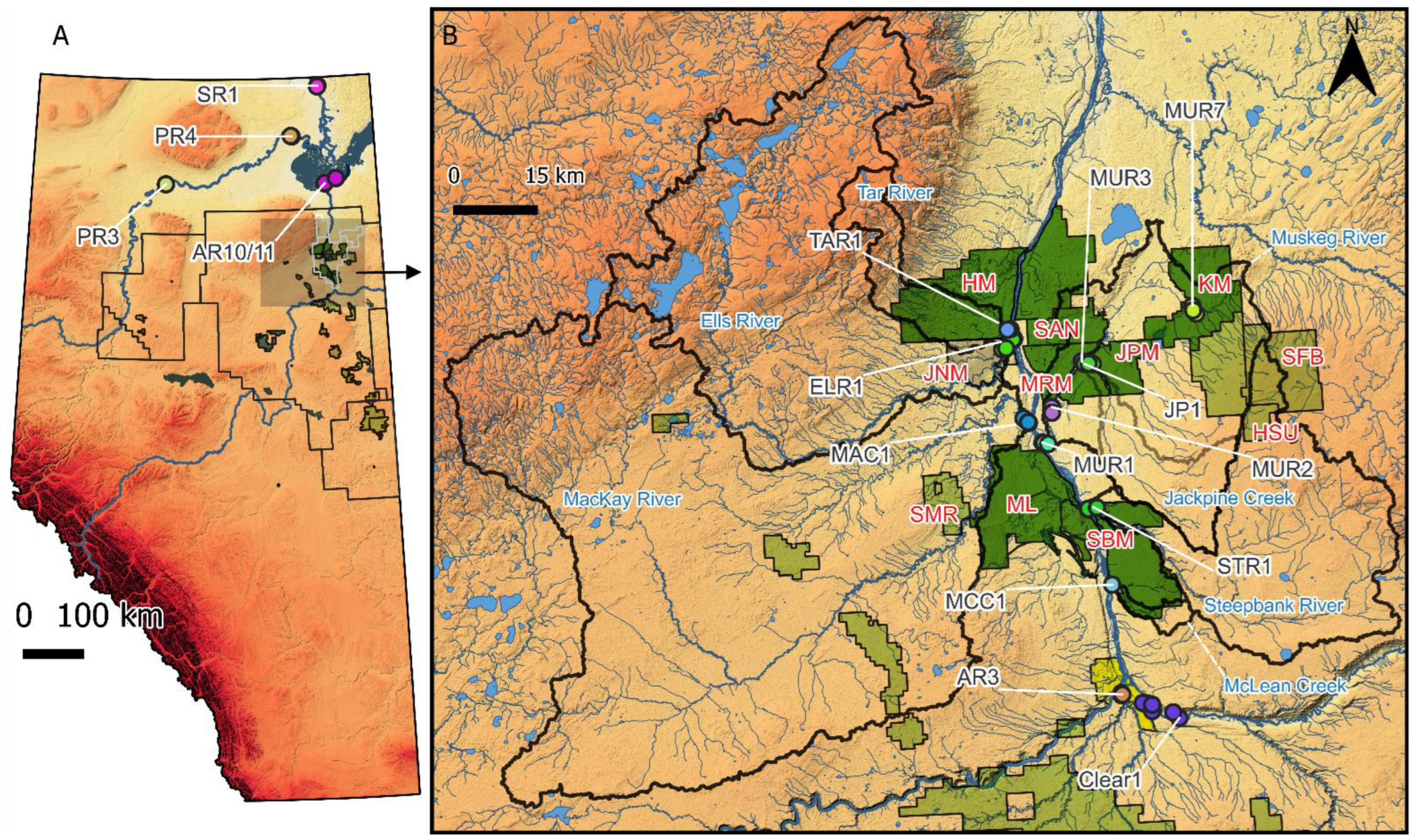
Using the long-term records available from multiple locations and the well-documented history of energy developments in northern Alberta, this study explored the concordance between known events and changes in residual conductivity (given alkalinity and other covariates) at sites over time. We compiled datasets from the long-term water quality records available in northern Alberta, including sites in the Muskeg, Steepbank, Tar, MacKay, and Ells rivers along with McLean and Jackpine creeks collected during multiple programs. We also obtained records from locations in the major regional rivers, the Athabasca, Peace, and Slave (Figure 1) and compiled histories of activities in the study area. These monitoring and activity data were compared to determine the potential utility of residual conductivity as a monitoring tool. We hypothesized residual conductivity would increase as human activity began or intensified in the respective watersheds.
2. Methods
2.1. Data Compilation and Preparation
We compiled specific conductance (µS/cm) and total alkalinity (as CaCO3 mg/L) data from 16 locations in northern Alberta, primarily from sites within the administratively defined Athabasca OSR (Figure 1). Specific conductance and total alkalinity are referred to herein as conductivity and alkalinity, respectively. Data for this work were obtained from several sources, including the Alberta long-term river network (LTRN) sites, the Alberta Oil Sands Environmental Research Program (AOSERP), the Regional Aquatics Monitoring Program (RAMP), the Joint Oil Sands Monitoring program (JOSM), and the Oil Sands Monitoring Program (OSM). We also considered data from pre-AOSERP records collected before 1976 [32]. Among the OSM and JOSM programs, the data were obtained from both the water quality and the benthic invertebrate programs.
The data used here are all publicly available on various Federal, e.g., [33] and Provincial Government, e.g., [34] portals. The most recent data for conductivity and alkalinity are available only rounded to the nearest 10 µS/cm or mg/L of CaCO3; this rounding was retrospectively applied to all data. Details of temporal changes in energy developments in the OSR tributaries was also extracted from the literature and from Google Earth imagery (Tables S1–S7).
While much sampling across years and the various programs has been performed at the same locations in the OSR tributaries, site coordinates fluctuated over time. Additionally, new sites may have been added while others were moved, or renamed. To extract the most information possible, general rules were established to amalgamate data from multiple sources and generate ‘sites’ for analysis here. These grouping rules included sites within ~5 river km, those with the same name, but slightly different coordinates, or those not separated by relevant features, such as road crossings or tributary confluences. The sites retained for analysis here were also prioritized. While data are available for more than 16 sites, we focused on locations with data collected before local oil sands industrial activities, but some sites without data before local development began, such as MCC1 were also retained. Blanks (field, trip, or lab) were removed from the dataset as were any duplicated records and samples missing either specific conductivity or total alkalinity. The final sample sizes of conductivity measurements for the 16 sites ranged from 27 (MCC1) to 571 (MUR2); Figure S2). The longest data record spans 1960–2018 and is from the SR1 location. The shortest record is from 1999–2016 and is from the MCC1 location.
2.2. Data Analyses
The amalgamation of data from multiple sources created two general challenges. First, many sources of covariation were present in the dataset, including different ‘types’ of reported specific conductance (i.e., lab, field, or not specified); some sites, including those in the Athabasca also used multiple sampling techniques (e.g., grabs, isokinetic samplers). Secondly, multiple frequencies of sample collections (e.g., hourly, daily, weekly, monthly, seasonally, and annual sampling campaigns) created complex autocorrelation structures within the compiled data sets. To overcome the statistical challenges embedded in the final water quality dataset, most notably including the covariates and the autocorrelation, we used Generalized Estimating Equations (GEE).
2.3. Generalized Estimating Equations
Generalized Estimating Equations are an extension of Generalized Linear Models used to analyze longitudinal and/or clustered data with correlated response measurements, e.g., [35]. The GEE models estimate the conditional mean and variance through an iteratively re-weighted least squares algorithm based on quasi-likelihood and sandwich estimators [36,37]. GEE is a marginal, population-averaged model and recommended where random effects are present, but specifying them is beyond the goals of the research [36,37]. Rather than specifying the random effects, GEE treats the covariance as a nuisance variable and eliminates it from the calculation of the regression coefficients [35]. While the standard errors are robust to misspecification of the correlation structures, correctly identifying them leads to greater efficiency [36]. Two major advantages of GEE for analyzing the current data set are accounting for unequal sampling intervals (eliminating the need to summarize correlated subsets of data, such as daily data, a priori, e.g., [38]) and fitting to non-normal data [35]. Consequently, all observations can be retained, including field duplicates and triplicates and no pre-transformations are necessary.
The GEEs were performed for each study location (since we were not interested in examining average responses across sites) using the ‘geeglm’ function in the ‘geepack’ package for R [39]. In this analysis, the data were fit using a Gamma distribution and the log-link function. While GEE is robust to a mis-specified working correlation structure, the autoregressive form (“ar1”), where data collected closer in time is more closely related, was the best conceptual match to the data [40]. The Quasi-Akaike’s Information Criterion (QIC; [41]) confirmed the appropriateness of the autocorrelation structure. The ‘waves’ argument was used to specify the unequal sampling intervals. Covariates beyond alkalinity, such as estimated discharge, mean precipitation, collection technique, and conductivity type were included in the analyses and are described in Appendix A. The results of the GEEs indicated significant relationships between conductivity and alkalinity supporting previous work (Tables S8 and S9; [30]). While the simplified QIC (QICu; [41]) indicated models without alkalinity typically performed better (Figure S3), the differences were minor and the variability of the models including alkalinity (compared to those without alkalinity; Figures S4 and S5) was smaller; consequently; alkalinity was retained. The GEE analysis estimated correlations of adjacent datapoints ranging from 0.94 at MUR2 to 0.19 at MCC1 (Table S10).
As explained in detail further below, the focus of this analysis is on the diagnostics of residuals estimated by the GEE models. While other sources of co-variation are possible, such as changes in measurement techniques of alkalinity or conductivity or over time, these sources, if systematic, contribute to residual variation in the model and, given the focus of the analysis here on residual diagnostics, increases its sensitivity. Including fac-tors such as program which did not vary randomly over time may also denude any relevant patterns. There is, however, some evidence suggesting some of these potential sources were not systematic across all sites; increasing, decreasing, and null trends in residual conductivity were also observed among locations suggesting there were little systematic influences of measurement techniques over time.
2.4. Data Interpretation
Residual diagnostics are a necessary, useful, and routine tool to identify, either qualitatively or quantitatively, additional structure remaining in a dataset analyzed using a statistical model [42]. Here, Pearson residuals from each of the GEEs were plotted over time to qualitatively determine the potential occurrence of relative changes associated with known events, such as the initial site preparation for a mine. We also used two locally weighted (LOESS) smoothers and one linear model to identify additional structural patterns in the residuals at various temporal scales but omitted their 95% Cis for clarity. The two LOESS smoothers were fit using the ’loess’ option in the ‘geom_smoother ()’ function in ggplot2 [43]. The first smoother was fit using an optimal and floating span calculated using the ‘optimal_span ()’ function in the ‘phenor’ Package [44] to identify the potential occurrence of changes over short periods. A second smoother using a span of 0.5 was also included in each plot to necessarily highlight longer-term trends in the data. To highlight general temporal patterns throughout the entire dataset, linear models were also fit to these data. Finally, a General Additive Model (GAM) smoother was also applied to residual conductivity using ggplot. Response residuals (observed minus expected) were also calculated to estimate the absolute change in conductivity (Figures S6 and S7).
Weighting was used to fit the LOESS and GAM smoothers and linear models. Weights were estimated for each data point based on when in time the previous data point was collected. The weights were derived from conductivity data collected at 15 min intervals with sondes deployed in the Firebag, Steepbank, and Ells rivers in the Spring and Summer of 2012, e.g., [33]. We extracted observations spaced by 24 h for the duration of the data period from these data for each site to calculate the autocorrelation functions between adjacent measurements. At these sites, a period of discernible autocorrelation ranged from 5–35 days (Figure S8). Weights for observations throughout the dataset were calculated as 1 minus the mean autocorrelation coefficients for all sites and a given day. Measurements collected more than 26 days after the previous measurement were set to a weight of 1.
Although the results focused on residual conductivity, two additional analyses were performed to evaluate the utility of this tool. First, residual conductivity was calculated without including alkalinity in the models. Second, time series plots of raw conductivity were also produced.
3. Results and Discussion
3.1. Potential Influence of Industrial Development in the Late 1970s and Early 1980s
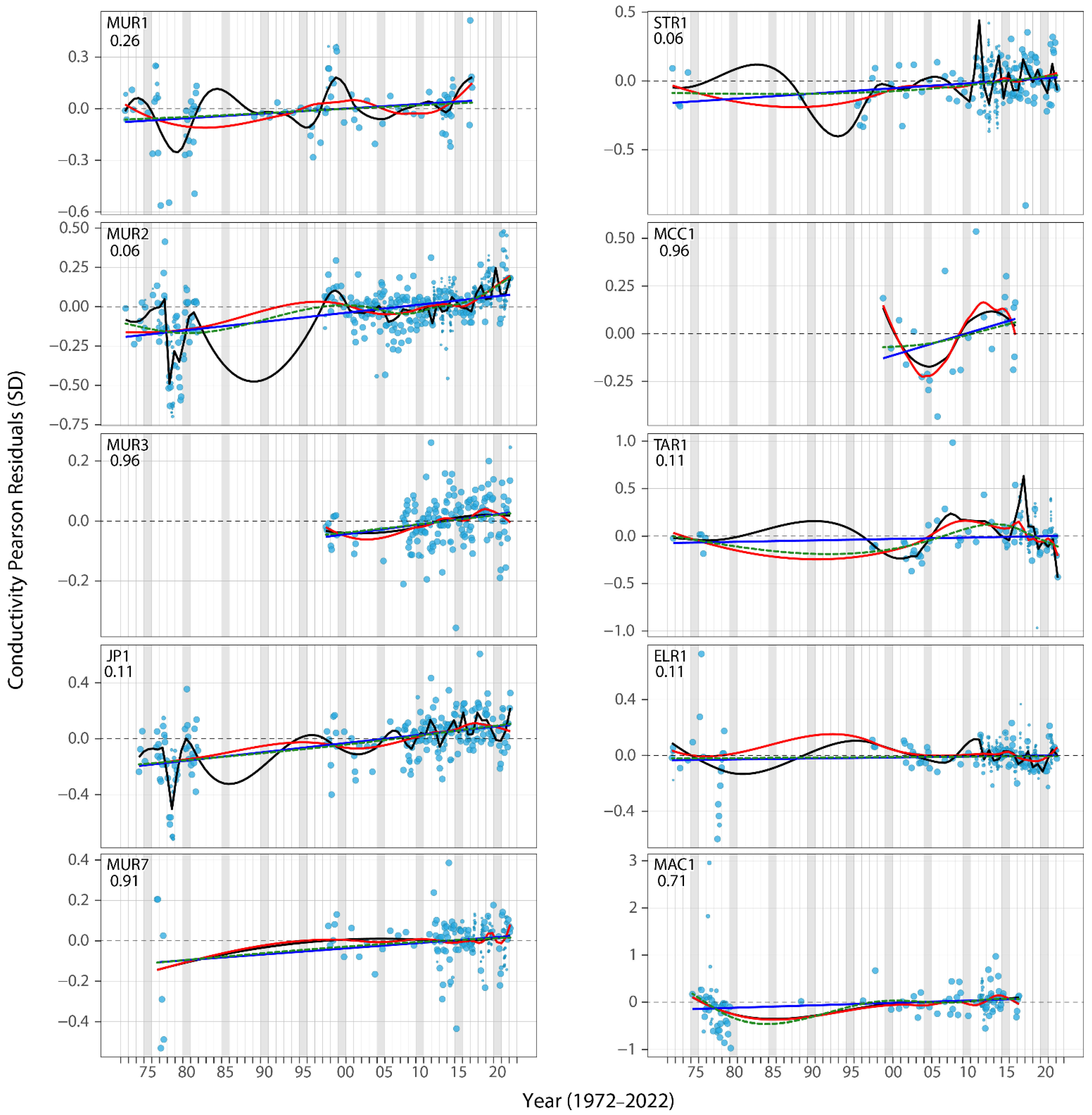
While pre-dated by other regional activities, including those at Bitumont [4], the earliest consistent (and large-scale) commercial activities in the OSR occurred at the Great Canadian Oil Sands (now Suncor Basemine) in 1967 and Syncrude Mildred Lake in 1978. Other exploratory activities also occurred in the Muskeg River basin in late 1970s, including road construction, land clearing and the construction of the 70 m ‘Shell test pit’ used to evaluate the feasibility of mining in the area [45]. Between 1976 and 1978, saline mine depressurization water was periodically discharged from the Shell test pit into the Muskeg River [29] and particulates were emitted from the Suncor coke-fired utility plant, although an electrostatic precipitator was installed and tested in the mid-1970s and brought fully online at this plant in November 1979 [46]. However, the efficiency of the precipitator was estimated at ~60% until at least 1980 [46]. Some of these activities may have affected residual conductivity in AOSR tributaries. While the chemistry of mine depressurization waters varies temporally and spatially [47,48], periodic discharges of these waters from the Shell test pit in the late 1970s may be apparent at the MUR2 and MUR1 locations as anomalously high residual conductivity, including September 1976 and July 1977 [29] (Figure 2).
While potential influences of discharges of depressurization waters from the Shell test pit are absent from Jackpine Creek, decreases in residual conductivity between 1977 and 1978 are common in the Muskeg drainage (MUR2, MUR7, and JP1; Figure 2). This pattern may also be present at other locations, such as SR1, PR4, STR1, ELR1, MAC1, TAR1, AR3, and Clear1 (Figure 2 and Figure 3). Some of the earliest patterns observed in residual conductivity during the 1970s and early 1980s may be partially related to the installation, testing, and operation of an electrostatic precipitator at the Great Canadian Oil Sands plant in the late 1970s, e.g., [46]. However, the parallel decline at AR3 suggests either the impacts of the emissions from Suncor were widespread, or other phenomena, such as any influence of the expansion of Fort McMurray may also be occurring. This pattern high-lights a general challenge in assessing impacts of specific activities in the OSR: driven by the price of oil, e.g., [25], industrial activity, including the initiation of projects and intensification of activities tends to be temporally clustered.
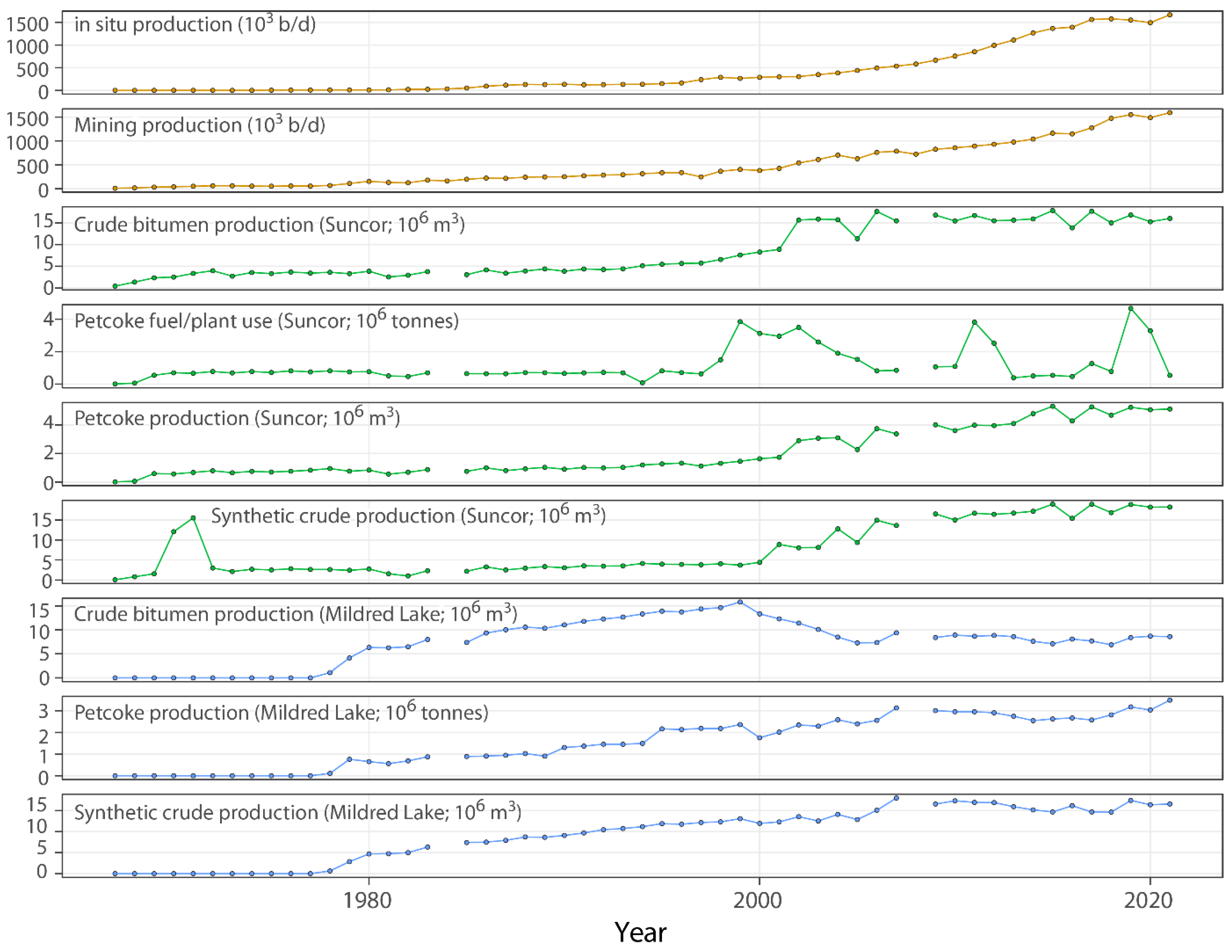
While reductions in conductivity in the late 1970s at some study sites, including some in the Muskeg basin may be related to early testing and commercial operation of the precipitator, later increases in 1980–1981 were also observed at the MUR2 location. These changes may also be related to the beginning of mining and the production of crude bitumen at the Mildred Lake facility and its later increases [49]. While the production increased from ~8000 m3 of bitumen in April of 1978 to between 215,000 and 252,000 m3 in October-December of the same year, synthetic crude production began at this facility in August 1978 (Figure 4); both increased between 1978 and 1980 at Mildred Lake. Particle deposition rates were also predicted to decrease after the installation of the precipitator at Suncor, but also increase with the opening of the Syncrude Mildred Lake facility [50]. While these data are not entirely consistent, they suggest the potential influence of changes in particulate metals associated with atmospheric emissions of oil sands industrial operations deposited on the landscape and washed into streams which have been challenging to identify, e.g., [51]. More specifically, synthetic crude production at Syncrude uses fluid coking and may be associated with increased loading of particulates to the landscape [52]. Loading of particulates from Suncor’s petroleum coke fired utility plant was well-known at the time [46,53] and may be responsible for increased metal loading in lake sediments, peat bogs, and snow near the emission sources and may also be associated with changes in fish health and benthic invertebrate communities [1,2,4,52,54,55,56,57]. Spatially, the inputs potentially associated with petroleum coke flyash into lakes were also restricted, e.g., [1]. The results from lake sediments are also temporally consistent with the appearance of signals in the lower Muskeg River (MUR1, MUR2, and JP1), but these three sites were also among those most intensively sampled during the 1970s; the potential occurrence of similar changes at additional locations is more challenging to identify.
While not definitive and challenging to verify, other observations also support a potential role of changes in atmospheric inputs on stream water chemistry. Reporting completed under AOSERP identified the potential influence of petroleum coke fly ash on ambient water and sediment chemistry, e.g., [58], but associations were not clearly demonstrated in earlier studies on flowing waters, e.g., [59]. Although the association between residual conductivity and petcoke combustion is tenuous, there is other data from the later 1990s and early 2000s may also indicate an effect of this stressor.
3.2. Additional Evidence of Petroleum Coke Fly Ash: Late 1990s and Early 2000s
While previous studies have suggested the potential associations of site preparation of the SAN and MRM and changes in water quality [3] (and construction schedules of oil sands facilities are commonly predicted in Environmental Impact Assessments, e.g., [60]), there is also some evidence suggesting increases in some metals, such as total vanadium in the late 1990s and early 2000s in the Muskeg River may also be at least partially associated with petroleum coke combustion at the Suncor utilities plant. While the various smoothers of residual conductivity collected at the MUR1 site from 1989 to 1997 suggests the potential presence of small increases, an increase in residual conductivity of ~150 µS/cm from 1996 to 1999 and then progressively falls to the pre-1996 value by ~2005 (Figure 2 and Figure S6). While there was no sampling at the MUR2 site from 1982–1997, the smoothers and residual conductivity at this site further suggest an increase at this site in the late 1990s (Figure 2). There is also some evidence suggesting this increase (and subsequent decrease) may have occurred at MUR3, JP1, MUR7, STR1, and MCC1, and weakly at MAC1, TAR1, and ELR1 (Figure 2).
The patterns in the residual conductivity from these locations, especially in tributaries east of the Athabasca River align with increases in petroleum coke use and combustion at the Suncor Basemine. From 1997 to 1999 the mass of petroleum coke combusted at Suncor increased by 6.11 times (Figure 4), but dropped from 1999 to 2006 (Figure 4). In contrast, other industrial metrics from facilities operating at this time (Suncor and Syncrude) did not show the abrupt spike in 1999 (Figure 4); crude bitumen production at Syncrude Mildred Lake peaked in 1999, but the increase was steady and occurred over a 20-year period. Petroleum coke combustion is associated with the emission of particulate metals, e.g., [46,52] and its influence has been suggested on lakes between Suncor and Syncrude and the south-eastern margins of the Muskeg drainage (and Jackpine sub-basin; [52]). Similarly, changes in particle size distributions in a bog in the Jackpine drainage also supports a potential role of petroleum coke combustion during this time [56]. As mentioned already, the combustion of petroleum coke at Suncor has also been identified as a likely contributor to the status of benthic invertebrates in streams throughout the region, including the lower Muskeg and Steepbank rivers, upper Jackpine Creek, and Shipyard Lake [54]. While an effect of a spike in the combustion and plant use of petroleum coke at Suncor in 2011 might also be apparent at some sites (MCC1, MUR2, and ELR1; Figure 2) and is also corroborated by data from bogs [56], this potential explanation is also consistent with the lack of discernible signals in indicator metals measured in the Muskeg River during the site preparation of the Jackpine and Kearl mines in 2006 and 2008, respectively [3]. However, improvements in environmental practices to reduce impacts during construction for these latter projects may also affect the patterns in data observed over time [4].
While increases in residual conductivity in 2019 at the MUR2 location may also be associated with increases in petroleum coke use at the Suncor Basemine in that year (Figure 2 and Figure 4), some data from the literature are not consistent with an effect of petroleum coke use at Suncor Basemine. Similarly, an increase in residual conductivity in late 2020 and early 2021 at the MUR2 location may not be associated with the use of petcoke at Suncor. Analyses of V from surface sediments collected over time from Shipyard Lake (located between the Steepbank River and McLean Creek watersheds) showed no positive associations with fuel and plant use of petroleum coke at Suncor [52]. The lack of associations at Shipyard Lake with fuel and plant use of petroleum coke at Suncor suggest a potential difference between rivers and lakes [61] or with no sampling of Shipyard Lake before 2001 [62]; the identification of an influence of fuel and plant use of petroleum coke at Suncor on benthic invertebrates in Shipyard Lake, e.g., [54] supports the latter. These observations suggest some of the potential relationships between residual conductivity and petcoke combustion are spurious, or may highlight changes in the relationships between industrial practices and environmental influences over time.
Although multiple stressors, including land disturbance [54] and inputs associated with other facilities [52] likely affect streams in the OSR, additional patterns may suggest a greater role of atmospheric deposition associated with petcoke combustion compared to site preparation. For example, the potential influence of fuel and plant use of petroleum coke at Suncor in ~1997–2006 may be apparent at multiple locations throughout the OSR (Figure 2) and the spike in residual conductivity is larger at the MUR1 location compared to the MUR2 site; MUR2 is closer to the SAN and MRM and both sites are downstream of the Alsands Drain [63]. While there is evidence of an influence of the discharge of waters from the Alsands Drain, residual conductivity suggests a potential relationship between water quality and combustion of petroleum coke at Suncor. Importantly, however, these data suggest a combination of tools is likely needed to identify the extent of industrial influence in the OSR; residual conductivity may be a useful part of the suite.
3.3. Local Development and Temporal Changes in Residual Conductivity
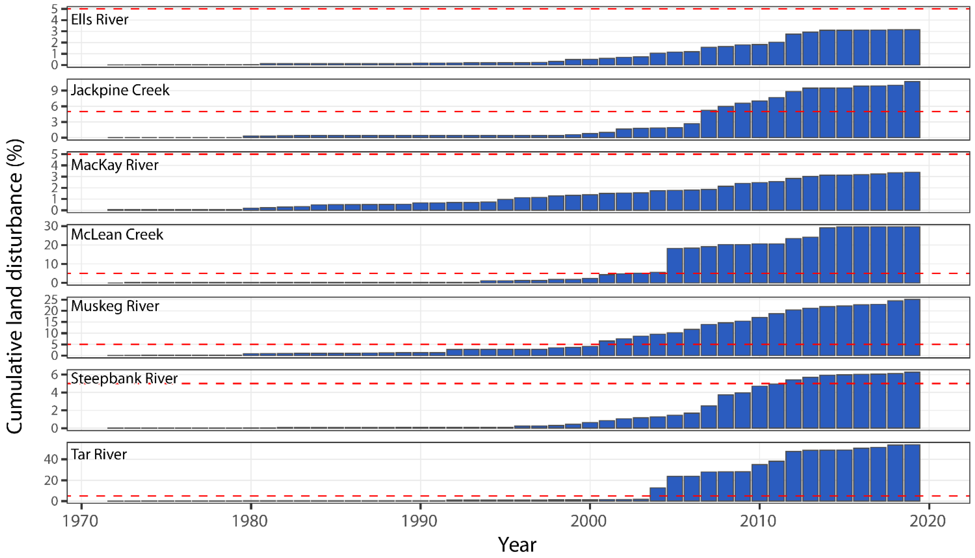
In contrast to the potential disappearance of the 1997–2002 spike in residual conductivity at MUR1 and MUR2 potentially associated with concurrent reductions of petroleum coke combustion or other phenomena, other activities have also occurred in the region. Some patterns in residual conductivity at multiple locations, such as variability at the STR1 location after ~2011 and increases between 2004 and 2008 in the Tar River (TAR1; Figure 2) suggest additional phenomena may also be affecting residual conductivity in the Athabasca tributaries. There may be some evidence of effects of site preparation and construction of both the JPM (2006–2010) and the KM (2008–2013) in residual conductivity in the Muskeg basin, including the MUR1, MUR2, and JP1 sites, but similar to other locations the variability in residual conductivity is challenging to clearly associate with the local developments. Later expansion and operation of the SAN, MRM, and JPM (opened commercially in 2010) mines, the Kearl mine (opened in 2013), the Hammerstone Quarry (constructed in 2006) and in situ activities (Suncor Firebag in 2004 and Husky Sunrise in 2015) comprising the progressive increase in land disturbance in the Muskeg River basin (and Jackpine sub-basin; Figure 5) may also be present as progressively greater conductivity than expected at the JP1, MUR2, MUR3, and less-so at the MUR7 site (Figure 2). Changes at these locations, such as MUR3, may also be influenced by the periodic and known discharges of mine depressurization water, clean-water runoff, storm water-runoff, or other waters into the Muskeg mainstem and Jackpine, Shelley, Muskeg, Stanley, and Wapasu Creeks since at least 2007, e.g., [62]. However, there are no clear relationships between known (but intermittent) discharges into Jackpine Creek (Figure S1) and residual conductivity at the JP1 site (Figure 2) in 2007–2009, 2013, and 2015, e.g., [62]. However, there are also long-term increases in residual conductivity at some sites and other shorter-term trends which may be associated with local developments and increases in production (Figure 2).
Although there may have been influence of particulate deposition on the STR1 site in the late 1990s, local land disturbances also occurred near the Steepbank River (but largely outside the basin) beginning in 1997 for the development of the Suncor Millennium Mine. In 2007, site preparation for the (north) Steepbank mine began and the first mine pit appeared in ~2013. Unlike the Millennium Mine, this later activity occurred within the Steepank basin and development of this project may be apparent at the STR1 location after 2010, but these changes may also be associated with increased sampling efforts (Figure 2).
While identifying sources of changes in residual conductivity and other water quality variables may typically be challenging in the OSR, some data may be more clearly associated with particular site preparation activities. For example, an increase in residual conductivity of roughly 20 µS/cm may have occurred in the at the TAR1 location between 2002 and 2009 (Figure 2; Figure S6). However, an increase of 215 µS/cm was observed at TAR1 between 2002 and 2008 (Figure 2; Figure S6). During this time, the Horizon Mine was being constructed in this basin and these changes in residual conductivity may reflect these activities. A similar increase in residual conductivity beginning in 2004/2005 in McLean Creek (Figure 2) and may also be associated with coinciding land disturbances within this basin (Figure 5). Although also potentially confounded by emissions from the Suncor coke-fired utilities plant, there is also some evidence from the MacKay (MAC1) River suggesting the influence of local development, including influence of Mildred Lake and SMR (Figure 2).
Although not definitive, there is also some evidence of a fewer changes in residual conductivity associated with development schedules in the Ells basin. First, construction of the Horizon Highway and traffic for the Horizon project after 2003 may have affected water quality in the Ells at the ELR1 site (Figure 2). While this signal may have faded by ~ 2006, later development activity in the Ells basin at the Joslyn North Mine site from 2010 to 2012 may have also led to the progressive increases in residual conductivity at the ELR1 location (Figure 2; e.g., [55]). Additionally, there was also potentially an effect of the 2014 abandonment of Joslyn North Mine at ELR1 (Figure 2). However, analyses of fish captured in the Ells basin also did not identify land disturbances as a driving factor, but did suggest the potential effects of atmospheric deposition [55] as did analyses in benthos [54].
While the results in this study cannot confirm how local development may affect streams, such as exacerbating deposition patterns or altering the mobilization of soils, clues to the relevance of these processes may be embedded in some of the existing data. For example, the patterns in residual conductivity suggest either the influence of local development via land disturbance and chemical weathering [64], local emissions [61,65], or global [66] atmospheric circulation and deposition, but also highlight potential complexities of identifying proximate causes. These data also support earlier contentions that materials derived from oil sands industrial activity, in this case, dissolved loads, are either retained in various land-forms, e.g., [1,5,67], are present but are occasionally [68] or commonly [69] obscured by natural signals and processes [70,71].
As also discussed below in the Slave River, some data from the OSR suggests land-scape disturbances may have a temporary effect on stream water chemistry. The impermanence of industrial signals may be associated with natural or artificial amelioration [6,72,73]. This is also demonstrated by the typically weak relationships between land disturbance and residual conductivity in the OSR (Figure S9). However, the weakness of relationships between stream water chemistry and land disturbance may also highlight the typical co-occurrence of multiple activities in the OSR and the overlapping effect path-ways linking industrial facilities with the ambient environment. Similar findings were reported in analyses of benthic invertebrates [54] and fish [55] suggesting measures of activity types and intensities are required.
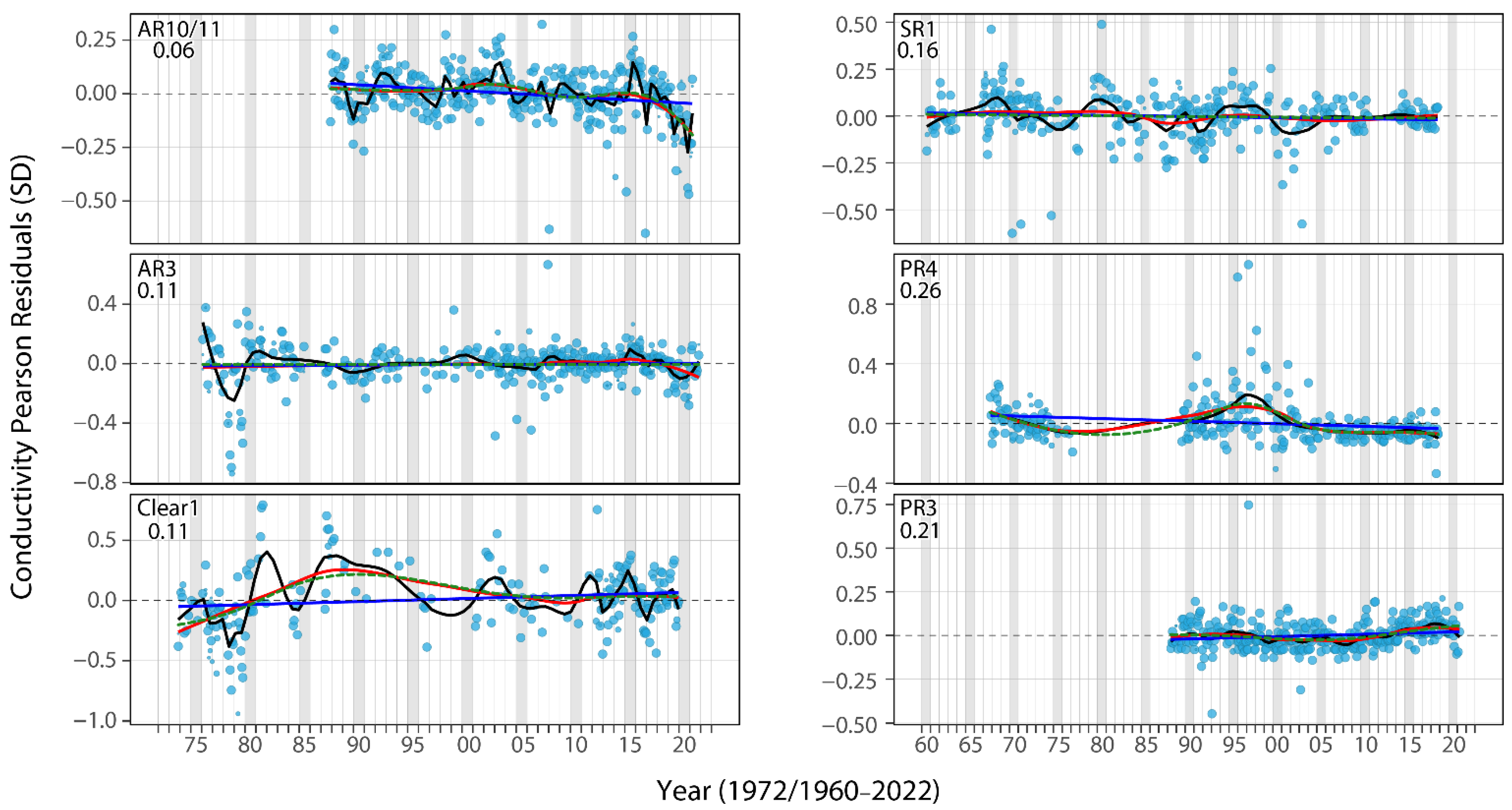
The analyses conducted here also support other information in the published literature. For example, there is evidence from additional locations of known spills in 1982 but not in 2007 ([63], and references therein) at the AR5 location (Figure S10). In contrast another potential event in the Spring of 1998 elevated residual conductivity at the AR9 (Figure S10) and AR10/11 locations (Figure 2), but small increases may also be present at the Clear1 site in 1998 (Figure 2). While no information on a spill in 1998 was found suggesting the high residual conductivity at AR9 in that year was not associated with an effect originating from oil sands facilities, an effect across multiple samples suggests a persistent phenomenon at that location while potential signals (although much smaller) at other sites (Clear1) also suggest some regional effect(s). However, these data (along with the potential relationship at AR5 in 1982 and a known spill and no evidence of others, such as the Obed dam breach in 2013 [73]) also highlight the well-known importance of sample timing, plume mixing, and natural amelioration on the detection of short-term events [73].
Additionally, in situ development may contribute contaminants of concern in lake sediments [74], but the patterns are not always apparent in metals [75]. While studies may not consider the effects of in situ developments, similar to other studies, e.g., [76], our results also suggest mines have a greater effect on the surrounding environment than in situ facilities. However, differences of individual operations within the ‘mining’ and ‘in situ’ extraction categories also likely contribute to the observed patterns [4,52].
3.4. Potential Influence of OSPW Seepage
Along with atmospheric deposition of particles and changes in air quality, the storage of Oil Sands Process-affected Water (OSPW) and its potential seepage from ponds are common concerns of local land and water users, e.g., [77]. Tailings ponds are either adjacent to or partially within the McClean Creek watershed and researchers suggest OSPW seepage may be present in this tributary [78,79], but this conclusion is not corroborated by compliance monitoring in groundwater monitoring wells [80]. However, increases in residual conductivity were found at the MCC1 site between ~2007 and 2014 and these changes may be associated with OSPW seepage. OSPW has a high content of dissolved solids [81] and this may affect the ratio of substances in stream water. Given the concentration of salts in the fluid, e.g., [82], and the use of dissolved components, such as salinity and ionic composition of groundwaters as a primary indicator that seepage may be present in monitoring wells [80], OSPW seepage may be detectable as a subtle increase in the mean residual conductivity. However, OSPW also contains dissolved organic com-pounds [83] and any potential seepage of this fluid and its resemblance when it reaches a surface water body [80] may have a complicated effect on residual conductivity in McLean Creek.
While greater rates of seepage are expected during the initial stages of pond use [84,85], the increase in residual conductivity between ~2007 and 2014 is not diagnostic. The pattern in residual conductivity at the MCC1 site could also indicate the influence of the diversion of McLean Creek (which may also contribute to increases in residual conductivity in the Tar River, especially in 2008), natural fluctuations and reversions to a long-term mean, or physical disruption of natural processes, such as the flow of brackish groundwaters [47,48,86,87]. However, McLean Creek has not been sampled since 2016. While any potential source of the change in residual conductivity at this site is speculative, the change may highlight the broad utility of this tool to launch additional focused studies to further evaluate the potential sources.
3.5. Potential Responses to Non-Oil Sands Stressors
Changes in residual conductivity in water from large river locations may also be as-sociated with human activities and support the wider utility of the tool. Among residuals from the SR1 site, there is potential evidence of change in the late 1960s and late 1970s/early 1980s coinciding with the respective openings of the Bennett and Peace Canyon dams (Figure 3). While no data prior to 1966 are available from the Peace River at Peace Point sampling location (PR4; Figure 3), a progressive decline in residual conductivity after 1968 at PR4 mirrors the decline observed at SR1 and supports the potential influence of the opening of the Bennett Dam and filling of Williston Lake. No data are available from either the PR3 or PR4 locations during the initialization of the Peace Canyon Dam (Figure 3) and this hypothesized mechanism cannot be evaluated for this additional facility.
Dams are expected to initially disrupt water quality, but the perturbations are also expected to eventually stabilize [6,88]. The residual conductivity data suggests evidence of these expected changes following the commercial operations of hydroelectric facilities on the Peace River. Importantly, earlier research did not suggest these impacts [7] and there is occasionally little to suggest changes in conductivity over time or residual conductivity calculated without alkalinity (Figures S11–S13). Most of the historical interest in the dams on the Peace River have addressed hydrological effects in the Peace-Athabasca Delta (PAD; e.g., [6]) and other physical implications of dam operation. The data examined here suggest a temporary influence role of initial damming and filling the reservoirs on dissolved loads in downstream areas. If real, these signals potentially persist for hundreds of km’s. Similar indications of long-range transport of organic contaminants originating from pulp mills and wood preservation facilities have also been observed in these same rivers [89]. However, the opening of Bennett and Peace Canyon dams also coincide with the respective openings of the Suncor Basemine and Syncrude’s Mildred Lake Mine (Figure 3). While not certain, there may be some influence of these oil sands facilities on residual conductivity at the SR1 site and others in the Athabasca River (Figure S10).
Evidence of the expansion of Fort McMurray may also be embedded in these analyses. Changes at AR3 and Clear1 in the 1970s and 1980s may be associated with the expansion of Fort McMurray [90] near both of these sites (Figure 1 and Figure 3). While later changes at some sites in the Athabasca River may also be associated with installation, operation, and alteration of municipal wastewater facilities [91], increases in residual conductivity in the Athabasca River corresponding to the start-up of pulp mills in the early 1990s, such as AR3 and AR10/11 [92] further suggests utility of this approach in augmenting other indicators of physicochemical influence, such as nutrient status [93].
Long-term declines in residual conductivity may also be present in the Athabasca River and reflect findings elsewhere [4,94]. Similar to the potential inputs associated with increases in particulates emitted from the combustion of petroleum coke at Suncor in some Athabasca tributaries, such as the Muskeg River, another common pattern in residual conductivity of large rivers was a transitory increase. Similar to data from the Muskeg River, signals of earlier industrial development in the 1960s and 1970s in the Slave River and the Athabasca River also appeared temporary (Figure 3). In many situations, physico-chemical recovery of water bodies is typical after large perturbations, e.g., [73], although the amelioration can occur over 1 to 2 decades [95], including areas where impacts on benthic invertebrates are common [96]. There is, however, also evidence of an unexplained drop in residual conductivity at the AR10/11 location over time and less so at the AR3 locations. Differences in long-term trends of residual conductivity at the AR10/11 location relative to AR3 and Clear1 may also be associated with effects of differences in physiography; the AR10/11 location is located within the physiographical boundary of the PAD (Figure 1).
Wildfires are also common in the boreal forest. Other work has identified changes in conductivity in streams of burned watersheds associated with precipitation and ash [97], but the analyses here suggest little influence of either the Richardson fire (2011) in the Muskeg River or the Horse River fire in the Steepbank River or McLean Creek watersheds (2016; Figure 2). Although sample timing may have missed relevant pulses, these results suggest residual conductivity may not be sensitive to changes in water quality associated with run-off events from burned watersheds.
3.6. Challenges with Residual Conductivity and Further Work
While many researchers have used ratios of chemical indicators, e.g., [1,5], and we show data suggesting the utility of residual conductivity to track anthropogenic influences in northern Alberta, there are also some challenges with this specific tool. While there is evidence suggesting the potential influence of known activities, or no differences with other events, there are some changes at multiple locations which are more challenging to reconcile. For example, increases in residual conductivity occurred at the AR10/11 and Clear1 locations between 2000 and 2005 and in 2015 (Figure 3). In contrast, an increase in residual conductivity is apparent at the PR4 location between ~1990 and 2005, but is less clear at the PR3 site (Figure 3). A decrease in residual conductivity after 2015 is also apparent at both the AR3 and AR10/11 locations, but not at the Clear1 site (Figure 3). These patterns suggest the potential influence of non-oil sands activities in upstream areas, but their specific origin is not clear. However, the changes may be associated with improvements in wastewater treatment or in changes in upstream land uses, including agriculture or wood harvesting and pulping, e.g., [98].
Additional comparisons using the raw conductivity measurements and conductivity models which do not include alkalinity (along with those that do) may also reveal additional information. For example, some indications of short-term changes at multiple locations, including potential increases in raw conductivity at sites in the Muskeg basin around 1999 are apparent, but longer-term trends may be absent; JP1 shows a long-term increase becomes more apparent as more covariates are included in the models (Figure 2, Figure S4, and Figure S12); a similar pattern also occurs at the MCC1 site, Figures S4 and S12). In contrast, decreases in raw conductivity and in Pearson residuals calculated from conductivity models which did not include alkalinity may, at the PR4 site, show greater potential associations with the initialization of the Bennett Dam located upstream (e.g., Figure 3 vs. Figures S5 and S13), but the same approach also showed less sensitivity at the SR1 location. Similarly, the positive slope of the linear model is also most apparent at the TAR1 location in the raw conductivity data over time (Figure S12) compared to, for example, the response residuals (Figure S6). These and other discrepancies in among the data, such as the potential effects of flow present in the raw conductivity data at the MUR3 site (Figure S12) and less apparent in residual conductivity (Figure 2) may highlight differences in the prevailing stressors and how they may affect stream conductivity, but also supports the need for suites of measurements to detect human influence typical of surveillance monitoring.
The analyses performed here were also retrospective and used data collected for multiple purposes. While these data may highlight some patterns, additional analyses are needed to verify the utility of residual conductivity as a tool for surveillance monitoring. A small-scale design conducted in sub-basins of tributaries, such as the Jackpine Creek watershed integrating all necessary measurements may be needed to disentangle the roles of various contributors in the OSR, e.g., [99]. Using smaller spatial scales for focused analyses is also advocated for detecting the occurrence of seepage from tailings ponds [78]. The roles of various contributors suggested here and elsewhere [54,55] may also be further tested using the planned expansions of existing facilities [55]. Based on the results here, we predict additional activities may, respectively, influence residual conductivity in the Ells and MacKay Rivers. Additionally, studies examining the potential toxicological implications of mine water return are currently underway, e.g., [100], but the field studies may be augmented by analyses of residual conductivity.
Although initial development in the Tar River and McLean Creek basins may have driven increases in residual conductivity, later increases in proportional land disturbances were not associated with continued increases in the indicator (Figure S9) and contrasts with observations in coal mining areas, e.g., [14]. While the differences between changes in conductivity measurements in coal mining areas, such as Appalachia and the Elk Valley and oil sands activity in northern Alberta may be associated with the different industrial practices, ore, volume and type of stockpiled materials, degree of hydrological isolation of project areas, or regulatory approaches [22,67,101], the results here suggest (as mentioned above) using proportional land disturbances in the OSR to estimate the degree of influence may also not account for the type of activities and changes in their intensity over time. For example, 17 of 30 tailings ponds present at mines in 2017 were constructed in mined-out pits [80]. In contrast, there is some evidence of positive long-term trends in the Muskeg basin (increase of ~125 µS/cm at the MUR2 location from the late 1970s to 2020–2022), suggesting there may be some associations with oil sands production [80] and land disturbance may identify these patterns.
A priority for monitoring the status surface waters in the OSR has been identifying a potential burst of toxicants delivered to streams during spring melt [26,51,102], but these influxes may not be clearly apparent in residual conductivity. However, while conductivity and alkalinity in snow from the OSR are typically low [103], increases in residual conductivity are also apparent in the spring of some years at some sites, such as MUR2 (Figure 2). These diffuse signals associated with concentration metrics uniquely related to oil sands industrial activities continue to be challenging to identify. Augmenting existing indicators of stress, such as decreases in pH [25] with residual conductivity may improve the separation of industrial impacts and natural influences of snowmelt on surface water bodies, e.g., [26]. Additionally, better understanding the behavior of residual conductivity with varying physical processes and materials using controlled laboratory experiments, e.g., [104] may offer great insight into the relationship explored here and compensate for the unavoidable inferential weaknesses of retrospective and observational studies [105]. However, residual conductivity may not be equally sensitive to all types of disturbances associated with human activities. For example, emissions of polycyclic aromatic compounds (PACs) have been associated with oil sands industrial activity, e.g., [106], but residual conductivity may be either insensitive or diminished by the known deposition of insoluble PACs, e.g., [61]. However, research suggests the electrical resistivity of hydrocarbons can change as parent materials are weathered and/or degraded in soils or other environmental reservoirs [107].
As mentioned already, the approach used here is likely best used as part of a suite of measurements. For example, ratios such as alkalinity and hardness, sodium to chloride, or others commonly used in environmental monitoring of groundwaters, e.g., [71]. Similarly, raw conductivity measurements, as discussed above, may also be suitable in many study environments, especially where watersheds can be instrumented, e.g., [22]. However, these chemical indicators may not address all of the potential information needs of managers and can also be combined with biomonitoring tools used in the area. The results of the studies on fish and benthic invertebrates suggest there is likely influence of industrial activities and some potentially large differences are present [54,55]. However, the most recently reported data (2012 to 2015) also suggests local streams were in good ecological condition [108].
4. Conclusions
Previous work suggests residual conductivity may be a useful tool for surveillance monitoring of streams. The analyses here compared residual conductivity at 16 stream sites to known human activities further supporting the utility of this tool. Residual conductivity suggests the potential influence of atmospheric deposition at multiple locations, including MUR2, site preparation at the TAR1 site, and the potential seepage of OSPW at the MCC1 location. There may also be evidence of large-scale hydroelectric development at the PR4 and SR1 locations and spills in the Athabasca. There are, however, some patterns in residual conductivity which may not be easily associated with activities, but may be worth additional analyses using other measurements also available from historical records. The approach likely has broad appeal and utility for surveillance monitoring of surface water bodies alongside other widely used techniques.
Supplementary Materials
The following supporting information can be downloaded at: https://www.mdpi.com/article/10.3390/w14162503/s1, references [55,94,109,110] are cited in the supplementary materials. Table S1: Owners of oil sands facilities, start-up years, and production capacity; obtained from Oil Sands Magazine (https://www.oilsandsmagazine.com/projects/bitumen-production); accessed on 17 November 2020; Table S2: History of activities in the Muskeg basin estimated from satellite imagery; Table S3: History of activities in the Steepbank basin estimated from satellite imagery; Table S4: History of activities in the McLean Creek basin estimated from satellite imagery; Table S5: History of activities in the MacKay River basin estimated from satellite imagery; Table S6: History of activities in the Ells River basin estimated from satellite imagery; Table S7: History of activities in the Tar River basin estimated from satellite imagery; Table S8: Summary Tables for tributary site GEEs; Table S9: Summary Tables for large river site GEEs; Table S10: Correlations of data estimated by the GEE using the ‘AR1′ working correlation structure; Figure S1: Locations of effluent discharges at oil sands facilities from 2012–2015 (purple, blue, red, yellow, respectively) obtained from Regional Aquatics Monitoring Program (RAMP) reports (RAMP 2016); HM = Horizon Mine; JNM = Joslyn North Mine; SMR= Suncor MacKay River; MLM = Mildred Lake Mine; SBM = Suncor Basemine; MM = Millennium Mine; NSM = North Steepbank Mine; JPM = Jackpine Mine; ANM = Aurora North Mine; MRM = Muskeg River Mine; FH = Fort Hills Mine; HS = Husky Sunrise; KM = Kearl Mine; Oil sands features layer from Oil Sands Information Portal (2016 data layer; http://osip.alberta.ca/library/Browser; accessed on 20 November 2021); also shown are the outlines of watershed boundaries (layer obtained from http://www.ramp-alberta.org/data/map/mapdata.aspx; accessed on 10 December 2021). Figure S2: Sample sizes per study location. Figure S3: Simplified QIC (QICu) calculated for models with and without alkalinity as an exploratory factor at the 16 sites examined in this study. Figure S4: Pearson residuals for conductivity models calculated without Alkalinity (SD) in tributaries of the Oil Sands Region draining to the Athabasca River. Points are individual observations scaled by mean autocorrelation factors (Figure S8) and lines show smoothers (LOESS: 0.5 span in red; optimal span (values below site names) in black; GAM in green dashing; linear model in blue); Site names correspond to locations shown in Figure 1. Figure S5: Pearson residuals for conductivity (SD) for large river lo-cations for models calculated without alkalinity; Points are individual observations scaled by mean autocorrelation factors (Figure S8) and lines show smoothers (LOESS: 0.5 span in red; optimal span (values below site names) in black; GAM in green dashing; linear model in blue); Site names correspond to locations shown in Figure 1. Figure S6: Response residuals for conductivity (µS/cm) in tributaries of the Oil Sands Region draining to the Athabasca River for models including alkalinity; points are individual observations scaled by mean autocorrelation factors (Figure S8) and lines show smoothers (LOESS: 0.5 span in red; optimal span (values below site names) in black; GAM in green dashing; linear model in blue); Site names correspond to locations shown in Figure 1. Figure S7: Response residuals for conductivity (µS/cm) in large river locations examined in this study using models with alkalinity; points are individual observations scaled by mean autocorrelation factors (Figure S8) and lines show smoothers (LOESS: 0.5 span in red; optimal span (values below site names) in black; GAM in green dashing; linear model in blue); Site names correspond to locations shown in Figure 1. Figure S8: Autocorrelation coefficients for samples separated by 24-h window from sondes deployed in 2013 in various tributaries; mean ACs used for weighting in smoothers; original data obtained from: http://donnees.ec.gc.ca/data/substances/monitor/surface-water-quality-oil-sands-region/tributary-water-quality-oil-sands-region/; accessed on 12 February 2021. Figure S9 Residual conductivity compared to cumulative land disturbance at locations near mouths of the Athabasca tributaries in the AOSR. Figure S10: Additional residual conductivity data from AR5 and AR9. Figure S11 Comparisons of raw conductivity, raw Alkalinity, and residual conductivity (with and without total Alkalinity (TA)) at the SR1 location (Slave River at Fitzgerald) from 1960–2018; two smoothers shown: solid blue line = optimal span smoother; dashed red line = 0.5 span smoother. Figure S12 Conductivity (µS/cm) in tributaries of the Oil Sands Region draining to the Athabasca River. Points are individual observations scaled by mean autocorrelation factors (Figure S8) and lines show smoothers (LOESS: 0.5 span in red; optimal span (values below site names) in black; GAM in green dashing; linear model in blue); Site names correspond to locations shown in Figure 1. Figure S13: Conductivity (µS/cm) in large river locations examined in this study. Points are individual observations scaled by mean autocorrelation factors (Figure S8) and lines show smoothers (LOESS: 0.5 span in red; optimal span (values below site names) in black; GAM in green dashing; linear model in blue); Site names correspond to locations shown in Figure 1.
Author Contributions
Conceptualization, T.J.A.; methodology, T.J.A.; formal analysis, T.J.A.; data curation, T.J.A.; writing—original draft preparation, T.J.A.; writing—review and editing, T.J.A. and D.R.R.; visualization, T.J.A. and D.R.R. All authors have read and agreed to the published version of the manuscript.
Funding
This research received no external funding.
Institutional Review Board Statement
Not applicable.
Informed Consent Statement
Not applicable.
Data Availability Statement
Data are available upon request.
Acknowledgments
Much work has been done, either historically or contemporaneously, to collect and analyze water samples and compile, store, analyze, interpret, house, and distribute the data. We acknowledge all the work from everyone involved in these sampling programs which provided the data on which this analysis is based and John Lakeman for moral support. This work does not necessarily reflect an official position of the Oil Sands Monitoring program or of Alberta Environment and Parks.
Conflicts of Interest
The authors salaries, which employed at Alberta Environment and Parks, was provided through the Oil Sands Monitoring program.
Appendix A
Supplemental methods describing covariates used in the analysis, including conductivity type, collection method, estimated discharge, and estimated precipitation.
References
- Cooke, C.A.; Kirk, J.L.; Muir, D.C.G.; Wiklund, J.A.; Wang, X.; Gleason, A.; Evans, M.S. Spatial and Temporal Patterns in Trace Element Deposition to Lakes in the Athabasca Oil Sands Region (Alberta, Canada). Environ. Res. Lett. 2017, 12, 124001. [Google Scholar] [CrossRef]
- Gopalapillai, Y.; Kirk, J.L.; Landis, M.S.; Muir, D.C.G.; Cooke, C.A.; Gleason, A.; Ho, A.; Kelly, E.; Schindler, D.; Wang, X.; et al. Source Analysis of Pollutant Elements in Winter Air Deposition in the Athabasca Oil Sands Region: A Temporal and Spatial Study. ACS Earth Space Chem. 2019, 3, 1656–1668. [Google Scholar] [CrossRef]
- Alexander, A.C.; Chambers, P.A. Assessment of Seven Canadian Rivers in Relation to Stages in Oil Sands Industrial Development, 1972–2010. Environ. Rev. 2016, 24, 484–494. [Google Scholar] [CrossRef]
- Arciszewski, T.J.; Hazewinkel, R.R.O.; Dubé, M.G. A Critical Review of the Ecological Status of Lakes and Rivers from Canada’s Oil Sands Region. Integr. Environ. Assess. Manag. 2022, 18, 361–387. [Google Scholar] [CrossRef] [PubMed]
- Shotyk, W.; Bicalho, B.; Cuss, C.; Donner, M.; Grant-Weaver, I.; Javed, M.B.; Noernberg, T. Trace Elements in the Athabasca Bituminous Sands: A Geochemical Explanation for the Paucity of Environmental Contamination by Chalcophile Elements. Chem. Geol. 2021, 581, 120392. [Google Scholar] [CrossRef]
- Prowse, T.D.; Beltaos, S.; Gardner, J.T.; Gibson, J.J.; Granger, R.J.; Leconte, R.; Peters, D.L.; Pietroniro, A.; Romolo, L.A.; Toth, B. Climate Change, Flow Regulation and Land-Use Effects on the Hydrology of the Peace-Athabasca-Slave System; Findings from the Northern Rivers Ecosystem Initiative. Environ. Monit. Assess. 2006, 113, 167–197. [Google Scholar] [CrossRef] [PubMed]
- Dubé, M.G.; Wilson, J.E. Accumulated State Assessment of the Peace-Athabasca-Slave River System. Integr. Environ. Assess. Manag. 2013, 9, 405–425. [Google Scholar] [CrossRef] [PubMed]
- Helsel, D.R. Statistics for Censored Environmental Data Using Minitab® and R: Second Edition; John Wiley & Sons: Hoboken, NJ, USA, 2011; Volume 77, ISBN 9780470479889. [Google Scholar]
- Donner, M.W.; Siddique, T. A Rapid and Sensitive IC-ICP-MS Method for Determining Selenium Speciation in Natural Waters. Can. J. Chem. 2018, 96, 795–802. [Google Scholar] [CrossRef]
- Shotyk, W.; Bicalho, B.; Cuss, C.W.; Donner, M.W.; Grant-Weaver, I.; Haas-Neill, S.; Javed, M.B.; Krachler, M.; Noernberg, T.; Pelletier, R.; et al. Trace Metals in the Dissolved Fraction (<0.45 mm) of the Lower Athabasca River: Analytical Challenges and Environmental Implications. Sci. Total Environ. 2017, 580, 660–669. [Google Scholar] [CrossRef] [PubMed]
- Debels, P.; Figueroa, R.; Urrutia, R.; Barra, R.; Niell, X. Evaluation of Water Quality in the Chillán River (Central Chile) Using Physicochemical Parameters and a Modified Water Quality Index. Environ. Monit. Assess. 2005, 110, 301–322. [Google Scholar] [CrossRef] [PubMed]
- Singh, S.; Hussian, A. Water Quality Index Development for Groundwater Quality Assessment of Greater Noida Sub-Basin, Uttar Pradesh, India. Cogent. Eng. 2016, 3, 1177155. [Google Scholar] [CrossRef]
- Lindberg, T.; Bernhardt, E.S.; Bier, R.; Helton, A.M.; Brittany Merola, R.; Vengosh, A.; di Giulio, R.T. Cumulative Impacts of Mountaintop Mining on an Appalachian Watershed. Proc. Natl. Acad. Sci. USA 2011, 108, 20929–20934. [Google Scholar] [CrossRef] [PubMed]
- Bernhardt, E.S.; Lutz, B.D.; King, R.S.; Fay, J.P.; Carter, C.E.; Helton, A.M.; Campagna, D.; Amos, J. How Many Mountains Can We Mine? Assessing the Regional Degradation of Central Appalachian Rivers by Surface Coal Mining. Environ. Sci. Technol. 2012, 46, 8115–8122. [Google Scholar] [CrossRef]
- Stets, E.G.; Kelly, V.J.; Crawford, C.G. Long-Term Trends in Alkalinity in Large Rivers of the Conterminous US in Relation to Acidification, Agriculture, and Hydrologic Modification. Sci. Total Environ. 2014, 488–489, 280–289. [Google Scholar] [CrossRef] [PubMed]
- Berger, E.; Haase, P.; Kuemmerlen, M.; Leps, M.; Schäfer, R.B.; Sundermann, A. Water Quality Variables and Pollution Sources Shaping Stream Macroinvertebrate Communities. Sci. Total Environ. 2017, 587–588, 1–10. [Google Scholar] [CrossRef] [PubMed]
- Cormier, S.M.; Zheng, L.; Hill, R.A.; Novak, R.M.; Flaherty, C.M. A Flow-Chart for Developing Water Quality Criteria from Two Field-Based Methods. Sci. Total Environ. 2018, 633, 1647–1656. [Google Scholar] [CrossRef] [PubMed]
- Hounslow, A. Water Quality Data: Analysis and Interpretation; CRC Press: Boca Raton, FL, USA, 2018; ISBN 1351404903. [Google Scholar]
- Erickson, R.J.; Nichols, J.W.; Cook, P.M.; Ankley, G.T. Bioavailability of Chemical Contaminants in Aquatic Systems. In The Toxicology of Fishes; CRC Press: London, UK, 2008; Volume 9, pp. 9–54. ISBN 9780203647295. [Google Scholar]
- Kleinow, K.M.; Nichols, J.W.; Hayton, W.L.; McKim, J.M.; Barron, M.G. Toxicokinetics in Fishes. In The Toxicology of Fishes; CRC Press: Boca Raton, FL, USA, 2008; pp. 55–152. [Google Scholar]
- Clements, W.H.; Kotalik, C. Effects of Major Ions on Natural Benthic Communities: An Experimental Assessment of the US Environmental Protection Agency Aquatic Life Benchmark for Conductivity. Freshw. Sci. 2016, 35, 126–138. [Google Scholar] [CrossRef]
- Griffith, M.B.; Norton, S.B.; Alexander, L.C.; Pollard, A.I.; LeDuc, S.D. The Effects of Mountaintop Mines and Valley Fills on the Physicochemical Quality of Stream Ecosystems in the Central Appalachians: A Review. Sci. Total Environ. 2012, 417–418, 1–12. [Google Scholar] [CrossRef]
- Armstead, M.Y.; Bitzer-Creathers, L.; Wilson, M. The Effects of Elevated Specific Conductivity on the Chronic Toxicity of Mining Influenced Streams Using Ceriodaphnia Dubia. PLoS ONE 2016, 11, e0165683. [Google Scholar] [CrossRef] [PubMed]
- Johnson, B.R.; Haas, A.; Fritz, K.M. Use of Spatially Explicit Physicochemical Data to Measure Downstream Impacts of Headwater Stream Disturbance. Water Resour. Res. 2010, 46, W09526. [Google Scholar] [CrossRef]
- Schindler, D.W. Geoscience of Climate and Energy 12. Water Quality Issues in the Oil Sands Region of the Lower Athabasca River, Alberta. Geosci. Can. 2013, 40, 202–214. [Google Scholar] [CrossRef]
- Alexander, A.C.; Chambers, P.A.; Jeffries, D.S. Episodic Acidification of 5 Rivers in Canada’s Oil Sands during Snowmelt: A 25-Year Record. Sci. Total Environ. 2017, 599–600, 739–749. [Google Scholar] [CrossRef]
- Headley, J.V.; Crosley, B.; Conly, F.M.; Quagraine, E.K. The Characterization and Distribution of Inorganic Chemicals in Tributary Waters of the Lower Athabasca River, Oilsands Region, Canada. J. Environ. Sci. Health Part A Toxic/Hazard. Subst. Environ. Eng. 2005, 40, 1–27. [Google Scholar] [CrossRef] [PubMed]
- Bodo, B.A. Statistical Analyses of Regional Surface Water Quality in Southeastern Ontario. Env. Monit Assess 1992, 23, 165–187. [Google Scholar] [CrossRef]
- Akena, A.M. An Intensive Surface Water Quality Study of the Muskeg River Watershed, Volume I; Alberta Environment and Sustainable Resource Development: Edmonton, AB, Canada, 1979.
- Proulx, C.L.; Kilgour, B.W.; Francis, A.P.; Bouwhuis, R.F.; Hill, J.R. Using a Conductivity–Alkalinity Relationship as a Tool to Identify Surface Waters in Reference Condition across Canada. Water Qual. Res. J. 2018, 53, 231–240. [Google Scholar] [CrossRef]
- Sechriest, R. Relationship Between Total Alkalinity, Conductivity, Original PH, and Buffer Action of Natural Water. Ohio J. Sci. 1960, 60, 303–308. [Google Scholar]
- Akena, A.M.; Christian, L. Water Quality of the Athabasca Oil Sands Area: Volume IV-an Interim Compilation of Non-AOSERP Water Quality Data; Alberta Oil Sands Environmental Research Program; Alberta Environment and Sustainable Resource Development: Edmonton, AB, Canada, 1981.
- Environment and Climate Change Canada Canada-Alberta Oil Sands Environmental Monitoring. Available online: https://www.canada.ca/en/environment-climate-change/services/oil-sands-monitoring.html (accessed on 20 July 2022).
- Kisters OSM Environmental Data Viewer. 2021. Available online: Https://Www.Canada.ca/En/Environment-Climate-Change/Services/Oil-Sands-Monitoring.Html (accessed on 20 July 2022).
- Liang, K.Y.; Zeger, S.L. Longitudinal Data Analysis Using Generalized Linear Models. Biometrika 1986, 73, 13–22. [Google Scholar] [CrossRef]
- Burton, P.; Gurrin, L.; Sly, P. Extending the Simple Linear Regression Model to Account for Correlated Responses: An Introduction to Generalized Estimating Equations and Multi-level Mixed Modelling. Stat. Med. 1998, 17, 1261–1291. [Google Scholar] [CrossRef]
- Ballinger, G.A. Using Generalized Estimating Equations for Longitudinal Data Analysis. Organ. Res. Methods 2004, 7, 127–150. [Google Scholar] [CrossRef]
- Morton, R.; Henderson, B.L. Estimation of Nonlinear Trends in Water Quality: An Improved Approach Using Generalized Additive Models. Water Resour. Res. 2008, 44, 1–11. [Google Scholar] [CrossRef]
- Halekoh, U.; Højsgaard, S.; Yan, J. The R Package Geepack for Generalized Estimating Equations. J. Stat. Softw. 2006, 15, 1–11. [Google Scholar] [CrossRef]
- Hardin, J.W.; Hilbe, J.M. Generalized Estimating Equations; CRC Press: London, UK, 2013. [Google Scholar]
- Cui, J.; Qian, G. Selection of Working Correlation Structure and Best Model in GEE Analyses of Longitudinal Data. Commun. Stat. Simul. Comput. 2007, 36, 987–996. [Google Scholar] [CrossRef]
- Harrell, F.E. Regression Modeling Strategies: With Applications to Linear Models, Logistic and Ordinal Regression, and Survival Analysis; Springer: Berlin/Heidelberg, Germany, 2015; ISBN 3319194259. [Google Scholar]
- Wickham, H.; Chang, W.; Wickham, M.H. Package ‘Ggplot2.’ Create Elegant Data Visualisations Using the Grammar of Graphics; CRAN: Indianapolis, IN, USA, 2016; Volume 2, pp. 1–189. [Google Scholar]
- Hufkens, K.; Basler, D.; Milliman, T.; Melaas, E.K.; Richardson, A.D. An Integrated Phenology Modelling Framework in R. Methods Ecol. Evol. 2018, 9, 1276–1285. [Google Scholar] [CrossRef]
- Alsands, P.G. Application to the Alberta Energy Resources Conservation Board for an Oil Sands Mining Project; Alberta Environment and Sustainable Resource Development: Edmonton, AB, Canada, 1978.
- Murray, W.A. The 1981 Snowpack Survey in the AOSERP Study Area; Alberta Environment and Sustainable Resource Development: Edmonton, AB, Canada, 1981.
- Rogers, W.; Lake, W. Acute Lethality of Mine Depressurization Water to Trout-Perch (Percopsis Omiscomaycus) and Rainbow Trout (Salmo Gairdneri) Volume II.; Alberta Environment and Sustainable Resource Development: Edmonton, AB, Canada, 1979.
- Lake, W.; Rogers, W. Acute Lethality of Mine Depressurization Water to Trout-Perch (Percopsis Omiscomaycus) and Rainbow Trout (Salmo Gairdneri) Volume I.; Alberta Environment and Sustainable Resource Development: Edmonton, AB, USA, 1979.
- AER ST39|Alberta Energy Regulator. Statistical Report 39. Available online: https://www.aer.ca/providing-information/data-and-reports/statistical-reports/st39 (accessed on 29 May 2021).
- Shelfentook, W. An Inventory System for Atmospheric Emissions in the AOSERP Study Area; SNC Tottrup Services Ltd.: Edmonton, AB, Canada, 1978. [Google Scholar]
- Wasiuta, V.; Kirk, J.L.; Chambers, P.A.; Alexander, A.C.; Wyatt, F.R.; Rooney, R.C.; Cooke, C.A. Accumulating Mercury and Methylmercury Burdens in Watersheds Impacted by Oil Sands Pollution. Environ. Sci. Technol. 2019, 53, 12856–12864. [Google Scholar] [CrossRef] [PubMed]
- Arciszewski, T.J. A Re-Analysis and Review of Elemental and Polycyclic Aromatic Compound Deposition in Snow and Lake Sediments from Canada’s Oil Sands Region Integrating Industrial Performance and Climatic Variables. Sci. Total Environ. 2022, 820, 153254. [Google Scholar] [CrossRef] [PubMed]
- Barrie, L.A.; Kovalick, J. A Wintertime Investigation of the Deposition of Pollutants around an Isolated Power Plant in Northern Alberta; Alberta Environment and Sustainable Resource Development: Edmonton, AB, Canada, 1980.
- Arciszewski, T.J. Exploring the Influence of Industrial and Climatic Variables on Communities of Benthic Macroinvertebrates Collected in Streams and Lakes in Canada’s Oil Sands Region. Environments 2021, 8, 123. [Google Scholar] [CrossRef]
- Arciszewski, T.J.; Ussery, E.J.; McMaster, M.E. Incorporating Industrial and Climatic Covariates into Analyses of Fish Health Indicators Measured in a Stream in Canada’s Oil Sands Region. Environments 2022, 9, 73. [Google Scholar] [CrossRef]
- Mullan-Boudreau, G.; Davies, L.; Devito, K.; Froese, D.; Noernberg, T.; Pelletier, R.; Shotyk, W. Reconstructing Past Rates of Atmospheric Dust Deposition in the Athabasca Bituminous Sands Region Using Peat Cores from Bogs. Land Degrad. Dev. 2017, 28, 2468–2481. [Google Scholar] [CrossRef]
- Mullan-Boudreau, G.; Belland, R.; Devito, K.; Noernberg, T.; Pelletier, R.; Shotyk, W. Sphagnum Moss as an Indicator of Contemporary Rates of Atmospheric Dust Deposition in the Athabasca Bituminous Sands Region. Environ. Sci. Technol. 2017, 51, 7422–7431. [Google Scholar] [CrossRef]
- Allan, R.; Jackson, T. Heavy Metals in Bottom Sediments of the Mainstem Athabasca River System in the AOSERP Study Area; Alberta Oil Sands Environmental Research Program; Alberta Environment and Sustainable Resource Development: Edmonton, AB, Canada, 1978. [CrossRef]
- Corkum, L. Water Quality of the Athabasca Oil Sands Area: A Regional Study; Alberta Environment and Sustainable Resource Development: Edmonton, AB, Canada, 1985. [CrossRef]
- Syncrude Canada. Environmental Impact Assessment for the Syncrude Aurora Mine; Syncrude Canada Ltd.: Edmonton, AB, Canada, 1996. [Google Scholar]
- Evans, M.; Davies, M.; Janzen, K.; Muir, D.; Hazewinkel, R.; Kirk, J.; de Boer, D. PAH Distributions in Sediments in the Oil Sands Monitoring Area and Western Lake Athabasca: Concentration, Composition and Diagnostic Ratios. Environ. Pollut. 2016, 213, 671–687. [Google Scholar] [CrossRef]
- RAMP Regional Aquatics Monitoring in Support of the Joint Oil Sands Monitoring Plan Final 2015 Program Report; AMERA: Edmonton, AB, Canada, 2016.
- Timoney, K.P.; Lee, P. Does the Alberta Tar Sands Industry Pollute? The Scientific Evidence. Open Conserv. Biol. J. 2009, 3, 65–81. [Google Scholar] [CrossRef]
- Javed, M.B.; Cuss, C.W.; Shotyk, W. Dissolved versus Particulate Forms of Trace Elements in the Athabasca River, Upstream and Downstream of Bitumen Mines and Upgraders. Appl. Geochem. 2020, 122, 104706. [Google Scholar] [CrossRef]
- Willis, C.E.; Kirk, J.L.; St Louis, V.L.; Lehnherr, I.; Ariya, P.A.; Rangel-Alvarado, R.B. Sources of Methylmercury to Snowpacks of the Alberta Oil Sands Region: A Study of in Situ Methylation and Particulates. Environ. Sci. Technol. 2018, 52, 531–540. [Google Scholar] [CrossRef] [PubMed]
- Shotyk, W.; Appleby, P.G.; Bicalho, B.; Davies, L.J.; Froese, D.; Grant-Weaver, I.; Magnan, G.; Mullan-Boudreau, G.; Noernberg, T.; Pelletier, R.; et al. Peat Bogs Document Decades of Declining Atmospheric Contamination by Trace Metals in the Athabasca Bituminous Sands Region. Environ. Sci. Technol. 2017, 51, 6237–6249. [Google Scholar] [CrossRef]
- Volik, O.; Elmes, M.; Petrone, R.; Kessel, E.; Green, A.; Cobbaert, D.; Price, J. Wetlands in the Athabasca Oil Sands Region: The Nexus between Wetland Hydrological Function and Resource Extraction. Environ. Rev. 2020, 28, 246–261. [Google Scholar] [CrossRef]
- Klemt, W.H.; Kay, M.L.; Wiklund, J.A.; Wolfe, B.B.; Hall, R.I. Assessment of Vanadium and Nickel Enrichment in Lower Athabasca River Floodplain Lake Sediment within the Athabasca Oil Sands Region (Canada). Environ. Pollut. 2020, 265, 114920. [Google Scholar] [CrossRef]
- Birks, S.J.; Cho, S.; Taylor, E.; Yi, Y.; Gibson, J.J. Characterizing the PAHs in Surface Waters and Snow in the Athabasca Region: Implications for Identifying Hydrological Pathways of Atmospheric Deposition. Sci. Total Environ. 2017, 603–604, 570–583. [Google Scholar] [CrossRef]
- Suzanne, C.L. Effects of Natural and Anthropogenic Non-Point Source Disturbances on the Structure and Function of Tributary Ecosystems in the Athabasca Oil Sands Region. Master’s Thesis, University of Victoria, Victoria, BC, Canada, 2015. [Google Scholar]
- Roy, J.W.; Bickerton, G.; Frank, R.A.; Grapentine, L.; Hewitt, L.M. Assessing Risks of Shallow Riparian Groundwater Quality near an Oil Sands Tailings Pond. Groundwater 2016, 54, 545–558. [Google Scholar] [CrossRef]
- Byrne, P.; Hudson-Edwards, K.A.; Bird, G.; Macklin, M.G.; Brewer, P.A.; Williams, R.D.; Jamieson, H.E. Water Quality Impacts and River System Recovery Following the 2014 Mount Polley Mine Tailings Dam Spill, British Columbia, Canada. Appl. Geochem. 2018, 91, 64–74. [Google Scholar] [CrossRef]
- Cooke, C.A.; Schwindt, C.; Davies, M.; Donahue, W.F.; Azim, E. Initial Environmental Impacts of the Obed Mountain Coal Mine Process Water Spill into the Athabasca River (Alberta, Canada). Sci. Total Environ. 2016, 557, 502–509. [Google Scholar] [CrossRef]
- Korosi, J.B.; Irvine, G.; Skierszkan, E.K.; Doyle, J.R.; Kimpe, L.E.; Janvier, J.; Blais, J.M. Localized Enrichment of Polycyclic Aromatic Hydrocarbons in Soil, Spruce Needles, and Lake Sediments Linked to in-Situ Bitumen Extraction near Cold Lake, Alberta. Environ. Pollut. 2013, 182, 307–315. [Google Scholar] [CrossRef] [PubMed]
- Skierszkan, E.K.; Irvine, G.; Doyle, J.R.; Kimpe, L.E.; Blais, J.M. Is There Widespread Metal Contamination from In-Situ Bitumen Extraction at Cold Lake, Alberta Heavy Oil Field? Sci. Total Environ. 2013, 447, 337–344. [Google Scholar] [CrossRef] [PubMed]
- Munkittrick, K.R.; Arciszewski, T.J. Using Normal Ranges for Interpreting Results of Monitoring and Tiering to Guide Future Work: A Case Study of Increasing Polycyclic Aromatic Compounds in Lake Sediments from the Cold Lake Oil Sands (Alberta, Canada) Described in Korosi et al. (2016). Environ. Pollut. 2017, 231, 1215–1222. [Google Scholar] [CrossRef] [PubMed]
- Gosselin, P.; Hrudey, S.E.; Naeth, M.A.; Plourde, A.; Therrien, R.; van der Kraak, G.; Xu, Z. Environmental and Health Impacts of Canada’s Oil Sands Industry; Royal Society of Canada: Ottawa, OT, USA, 2010; p. 438. [Google Scholar]
- Sun, C.; Shotyk, W.; Cuss, C.W.; Donner, M.W.; Fennell, J.; Javed, M.; Noernberg, T.; Poesch, M.; Pelletier, R.; Sinnatamby, N.; et al. Characterization of Naphthenic Acids and Other Dissolved Organics in Natural Water from the Athabasca Oil Sands Region, Canada. Environ. Sci. Technol. 2017, 51, 9524–9532. [Google Scholar] [CrossRef]
- Ross, M.S.; Pereira, A.D.S.; Fennell, J.; Davies, M.; Johnson, J.; Sliva, L.; Martin, J.W. Quantitative and Qualitative Analysis of Naphthenic Acids in Natural Waters Surrounding the Canadian Oil Sands Industry. Environ. Sci. Technol. 2012, 46, 12796–12805. [Google Scholar] [CrossRef]
- Fennell, J.; Arciszewski, T.J. Current Knowledge of Seepage from Oil Sands Tailings Ponds and Its Environmental Influence in Northeastern Alberta. Sci. Total Environ. 2019, 686, 968–985. [Google Scholar] [CrossRef]
- Allen, E.W. Process Water Treatment in Canada’s Oil Sands Industry: II. A Review of Emerging Technologies. J. Environ. Eng. Sci. 2008, 7, 499–524. [Google Scholar] [CrossRef]
- McQueen, A.D.; Kinley, C.M.; Hendrikse, M.; Gaspari, D.P.; Calomeni, A.J.; Iwinski, K.J.; Castle, J.W.; Haakensen, M.C.; Peru, K.M.; Headley, J.V.; et al. A Risk-Based Approach for Identifying Constituents of Concern in Oil Sands Process-Affected Water from the Athabasca Oil Sands Region. Chemosphere 2017, 173, 340–350. [Google Scholar] [CrossRef]
- Frank, R.A.; Bauer, A.E.; Roy, J.W.; Bickerton, G.; Rudy, M.D.; Vanderveen, R.; Batchelor, S.; Barrett, S.E.; Milestone, C.B.; Peru, K.M.; et al. Preparative Isolation, Fractionation and Chemical Characterization of Dissolved Organics from Natural and Industrially Derived Bitumen-Influenced Groundwaters from the Athabasca River Watershed. Sci. Total Environ. 2021, 777, 146022. [Google Scholar] [CrossRef]
- Ferguson, G.P.; Rudolph, D.L.; Barker, J.F. Hydrodynamics of a Large Oil Sand Tailings Impoundment and Related Environmental Implications. Can. Geotech. J. 2009, 46, 1446–1460. [Google Scholar] [CrossRef]
- Atkinson, J.M.; Bouthillier, P.H.; Gallup, D.N.; Greenhill, S.; MacKay, W.E.; Morgenstern, N.R. Great Canadian Oil Sands Dyke Discharge Water. Summary Report of the Scientific Enquiry Committee; Alberta Environment and Sustainable Resource Development: Edmonton, AB, Canada, 1976.
- Gibson, J.J.; Yi, Y.; Birks, S.J. Isotope-Based Partitioning of Streamflow in the Oil Sands Region, Northern Alberta: Towards a Monitoring Strategy for Assessing Flow Sources and Water Quality Controls. J. Hydrol. Reg. Stud. 2016, 5, 131–148. [Google Scholar] [CrossRef]
- Cumulative Environmental Management Association (CEMA). Review of Potential Cumulative Impacts to Surface Water and Groundwater from Current and Proposed In-Situ Oil Sands Operations; CEMA: Edmonton, AB, Canada, 2014. [Google Scholar]
- Prowse, T.D.; Conly, F.M. A Review of Hydroecological Results of the Northern River Basins Study, Canada. Part 2. Peace-Athabasca Delta. River Res. Appl. 2002, 18, 447–460. [Google Scholar] [CrossRef]
- McMaster, M.E.; Evans, M.S.; Alaee, M.; Muir, D.C.G.; Hewitt, L.M. Northern Rivers Ecosystem Initiative: Distribution and Effects of Contaminants. Environ. Monit. Assess. 2006, 113, 143–165. [Google Scholar] [CrossRef] [PubMed]
- Smith, S.B. Alberta Oil Sands Environmental Research Program 1975-1980: Summary Report; Alberta Oil Sands Environmental Research Program; Alberta Environment and Sustainable Resource Development: Calgary, AB, Canada, 1981.
- Arciszewski, T.J.; McMaster, M.E. Potential Influence of Sewage Phosphorus and Wet and Dry Deposition Detected in Fish Collected in the Athabasca River North of Fort Mcmurray. Environement 2021, 8, 14. [Google Scholar] [CrossRef]
- Squires, A.J.; Dubé, M.G. Development of an Effects-Based Approach for Watershed Scale Aquatic Cumulative Effects Assessment. Integr Env. Assess Manag 2013, 9, 380–391. [Google Scholar] [CrossRef] [PubMed]
- Scrimgeour, G.J.; Chambers, P.A. Cumulative Effects of Pulp Mill and Municipal Effluents on Epilithic Biomass and Nutrient Limitation in a Large Northern River Ecosystem. Can. J. Fish. Aquat. Sci. 2000, 57, 1342–1354. [Google Scholar] [CrossRef]
- Arciszewski, T.J.; Hazewinkel, R.R.; Munkittrick, K.R.; Kilgour, B.W. Developing and Applying Control Charts to Detect Changes in Water Chemistry Parameters Measured in the Athabasca River near the Oil Sands: A Tool for Surveillance Monitoring. Environ. Toxicol. Chem. 2018, 37, 2296–2311. [Google Scholar] [CrossRef]
- Evans, D.M.; Zipper, C.E.; Donovan, P.F.; Daniels, W.L. Long-Term Trends of Specific Conductance in Waters Discharged by Coal-Mine Valley Fills in Central Appalachia, USA. JAWRA J. Am. Water Resour. Assoc. 2014, 50, 1449–1460. [Google Scholar] [CrossRef]
- Pond, G.J.; Passmore, M.E.; Pointon, N.D.; Felbinger, J.K.; Walker, C.A.; Krock, K.J.G.; Fulton, J.B.; Nash, W.L. Long-Term Impacts on Macroinvertebrates Downstream of Reclaimed Mountaintop Mining Valley Fills in Central Appalachia. Environ. Manag. 2014, 54, 919–933. [Google Scholar] [CrossRef]
- Emmerton, C.A.; Cooke, C.A.; Hustins, S.; Silins, U.; Emelko, M.B.; Lewis, T.; Kruk, M.K.; Taube, N.; Zhu, D.; Jackson, B.; et al. Severe Western Canadian Wildfire Affects Water Quality Even at Large Basin Scales. Water Res. 2020, 183, 116071. [Google Scholar] [CrossRef]
- Dubé, M.; Johnson, B.; Dunn, G.; Culp, J.; Cash, K.; Munkittrick, K.; Wong, I.; Hedley, K.; Booty, W.; Lam, D.; et al. Development of a New Approach to Cumulative Effects Assessment: A Northern River Ecosystem Example. Environ. Monit. Assess. 2006, 113, 87–115. [Google Scholar] [CrossRef] [PubMed]
- Arciszewski, T.J.; Roberts, D.R.; Munkittrick, K.R.; Scrimgeour, G.J. Challenges and Benefits of Approaches Used to Integrate Regional Monitoring Programs. Front. Environ. Sci. 2021, 9, 256. [Google Scholar] [CrossRef]
- Hicks, K.; Scrimgeour, G. A Study Design for Enhanced Environmental Monitoring of the Lower Athabasca River; Office of the Chief Scientist, Ministry of Environment and Parks: Edmonton, AB, Canada, 2019; ISBN 1460145364.
- Wellen, C.; Shatilla, N.J.; Carey, S.K. The Influence of Mining on Hydrology and Solute Transport in the Elk Valley, British Columbia, Canada. Environ. Res. Lett. 2018, 13, 074012. [Google Scholar] [CrossRef]
- Birks, S.J.; Moncur, M.C.; Gibson, J.J.; Yi, Y.; Fennell, J.W.; Taylor, E.B. Origin and Hydrogeological Setting of Saline Groundwater Discharges to the Athabasca River: Geochemical and Isotopic Characterization of the Hyporheic Zone. Appl. Geochem. 2018, 98, 172–190. [Google Scholar] [CrossRef]
- Parrott, J.L.; Marentette, J.R.; Hewitt, L.M.; McMaster, M.E.; Gillis, P.L.; Norwood, W.P.; Kirk, J.L.; Peru, K.M.; Headley, J.V.; Wang, Z.; et al. Meltwater from Snow Contaminated by Oil Sands Emissions Is Toxic to Larval Fish, but Not Spring River Water. Sci. Total Environ. 2018, 625, 264–274. [Google Scholar] [CrossRef] [PubMed]
- Daniels, W.L.; Zipper, C.E.; Orndorff, Z.W.; Skousen, J.; Barton, C.D.; McDonald, L.M.; Beck, M.A. Predicting Total Dissolved Solids Release from Central Appalachian Coal Mine Spoils. Environ. Pollut. 2016, 216, 371–379. [Google Scholar] [CrossRef]
- Platt, J.R. Strong Inference: Certain Systematic Methods of Scientific Thinking May Produce Much More Rapid Progress than Others. Science 1964, 146, 347–353. [Google Scholar] [CrossRef] [PubMed]
- Kurek, J.; Kirk, J.L.; Muir, D.C.G.G.; Wang, X.; Evans, M.S.; Smol, J.P. Legacy of a Half Century of Athabasca Oil Sands Development Recorded by Lake Ecosystems. Proc. Natl. Acad. Sci. USA 2013, 110, 1761–1766. [Google Scholar] [CrossRef]
- Atekwana, E.A.; Atekwana, E.A.; Rowe, R.S.; Werkema, D.D.; Legall, F.D. The Relationship of Total Dissolved Solids Measurements to Bulk Electrical Conductivity in an Aquifer Contaminated with Hydrocarbon. J. Appl. Geophys. 2004, 56, 281–294. [Google Scholar] [CrossRef]
- Culp, J.M.; Glozier, N.E.; Baird, D.J.; Wrona, F.J.; Brua, R.B.; Ritcey, A.L.; Peters, D.L.; Choung, C.B.; Curry, C.J. Assessing Ecosystem Health in Benthic Macroinvertebrate Assemblages of the Athabasca River Main Stem, Tributaries and Peace-Athabasca Delta; Government of Alberta: Edmonton, AB, Canada, 2018.
- Arciszewski, T.J.; Munkittrick, K.R.; Scrimgeour, G.J.; Dubé, M.G.; Wrona, F.J.; Hazewinkel, R.R. Using Adaptive Processes and Adverse Outcome Pathways to Develop Meaningful, Robust, and Actionable Environmental Monitoring Programs. Integr. Environ. Assess. Manag. 2017, 13, 877–891. [Google Scholar] [CrossRef]
- Glozier, N.E.; Pippy, K.; Levesque, L.; Ritcey, A.; Armstrong, B.; Tobin, O.; Cooke, C.A.; Conly, M.; Dirk, L.; Epp, C.; et al. Surface Water Quality of the Athabasca, Peace and Slave Rivers and Riverine Waterbodies within the Peace-Athabasca Delta; Oil Sands Monitoring Program Technical Report Series No. 1.4; Alberta Environment and Parks: Edmonton, AB, Canada, 2018; ISBN 9781460140284. [Google Scholar]
Figure 1.
Maps of study area including all 14 locations and industrial project areas (dark green = mines; light green = in situ; grey = paused); (A) study locations outside the administrative Oil Sands Areas (black lines) and the minable sub-region (while lines); (B) study locations inside and adjacent to the minable region within the Athabasca Oil Sands Region; boundaries of the Tar, Ells, MacKay, Muskeg, and Steepbank rivers, and Jackpine and McLean creeks; original coordinates of all sampling locations were retained and grouped by colors; land disturbance data omitted for clarity; Fort McMurray shown in yellow; only names of relevant projects shown in red text: HM = Horizon mine; SAN = Syncrude Aurora North; KM = Kearl Mine; SFB = Suncor Firebag; HSU = Husky Sunrise; SBM = Suncor Basemine; ML = Mildred Lake; SMR = Suncor MacKay River; MRM = Muskeg River Mine; JNM = Joslyn North Mine; JPM = Jackpine Mine; additional details available in Figure S1.

Figure 2.
Pearson residuals (±Standard Deviation) of conductivity measurements in tributaries of the Oil Sands Region draining to the Athabasca River. Points are individual observations scaled by mean autocorrelation factors (Figure S8) and lines show smoothers (LOESS: 0.5 span in red; optimal span (values below site names) in black; GAM in green dashing; linear model in blue); site names correspond to locations shown in Figure 1.

Figure 3.
Pearson residuals (±Standard Deviation) of conductivity measurements in large river sites in norther Alberta; points are individual observations scaled by mean autocorrelation factors (Figure S8) and lines show smoothers (LOESS: 0.5 span in red; optimal span (values below site names) in black; GAM in green dashing; linear model in blue); site names correspond to locations in Figure 1.

Figure 4.
Annual production for in situ and mining sectors along with and performance metrics from Suncor Basemine (Suncor) and Syncrude Mildred Lake from 1967 to 2021; facility-specific performance data from 1984 and 2008 not available.
Figure 4.
Annual production for in situ and mining sectors along with and performance metrics from Suncor Basemine (Suncor) and Syncrude Mildred Lake from 1967 to 2021; facility-specific performance data from 1984 and 2008 not available.

Figure 5.
Estimated cumulative land disturbances (%) of total watershed area in the Ells, MacKay, Muskeg, Steepbank, and Tar rivers and Jackpine and McLean Creek since 1970; horizontal dashed red line marks 5.4% cumulative land disturbance identified as a critical threshold in [14].
Figure 5.
Estimated cumulative land disturbances (%) of total watershed area in the Ells, MacKay, Muskeg, Steepbank, and Tar rivers and Jackpine and McLean Creek since 1970; horizontal dashed red line marks 5.4% cumulative land disturbance identified as a critical threshold in [14].

Publisher’s Note: MDPI stays neutral with regard to jurisdictional claims in published maps and institutional affiliations. |
© 2022 by the authors. Licensee MDPI, Basel, Switzerland. This article is an open access article distributed under the terms and conditions of the Creative Commons Attribution (CC BY) license (https://creativecommons.org/licenses/by/4.0/).
Share and Cite
MDPI and ACS Style
Arciszewski, T.J.; Roberts, D.R. Analyzing Relationships of Conductivity and Alkalinity Using Historical Datasets from Streams in Northern Alberta, Canada. Water 2022, 14, 2503. https://doi.org/10.3390/w14162503
AMA Style
Arciszewski TJ, Roberts DR. Analyzing Relationships of Conductivity and Alkalinity Using Historical Datasets from Streams in Northern Alberta, Canada. Water. 2022; 14(16):2503. https://doi.org/10.3390/w14162503
Chicago/Turabian StyleArciszewski, Tim J., and David R. Roberts. 2022. "Analyzing Relationships of Conductivity and Alkalinity Using Historical Datasets from Streams in Northern Alberta, Canada" Water 14, no. 16: 2503. https://doi.org/10.3390/w14162503
Note that from the first issue of 2016, this journal uses article numbers instead of page numbers. See further details here.