Article

Spatiotemporal Variations in Reference Evapotranspiration and Its Contributing Climatic Variables at Various Spatial Scales across China for 1984–2019

1
School of Water Resources Engineering, Dalian University of Technology, 2 Ling Gong Road, Dalian 116024, China
2
Department of Civil Engineering, University of Ottawa, 161 Louis Pasteur, Ottawa, ON K1N 6N5, Canada
*
Author to whom correspondence should be addressed.
Water 2022, 14(16), 2502; https://doi.org/10.3390/w14162502
Submission received: 19 June 2022 / Revised: 2 August 2022 / Accepted: 11 August 2022 / Published: 14 August 2022

Abstract

:
Reference evapotranspiration (ET0) is of great significance in studies of hydrological cycle, agricultural water resources, and hydrometeorology. The present study collected daily meteorological data at 536 meteorological stations in China from 1984 to 2019, calculated daily ET0 using the FAO Penman–Monteith equation, analyzed the spatial distribution and temporal variation characteristics of ET0 and meteorological variables at four different spatial scales (continental, regional, provincial, and local), and discussed the sensitivity of ET0 to the meteorological variables and the contribution rates of the meteorological variables to the ET0 variations. The results showed that ET0 increased at 406 out of the 536 stations (75.7%), with the trends being significant at 65 stations at the 5% significance level, and 147 at the 1% significance level. The slope calculated using Sen’s method and linear trend method showed that the annual ET0 at the continental scale increased by approximately 12 mm/decade. Most of the stations showed decreasing trends in relative humidity (Hm), sunshine duration (SD), and wind speed at 2 m height (U2) while increasing trends in the maximum air temperature (Tmax) and minimum air temperature (Tmin). ET0 was most sensitive to Hm (sensitivity coefficient, St = −0.66), followed by Tmax (St = 0.29), SD (St = 0.18), U2 (St = 0.16), and Tmin (St = 0.07). Most of the stations showed increasing trends in St for Hm (56.16%), Tmax (72.95%), Tmin (87.31%), and U2 (90.49%), and decreasing trends for SD (69.78%). The variations in Hm, Tmax, and Tmin increased the ET0 at most of the stations (82.28%, 98.13%, and 69.03%, respectively). The variations in SD and U2 decreased ET0 at most of the stations (66.04% and 56.34%, respectively). Some ET0 characteristics in a few regions can be well described using a single spatial scale. However, most regions exhibited significantly different ET0 characteristics across spatial scales. The results of this project can provide reference for hydrological analysis and agricultural water management under climate change conditions and provide data and information for other hydrology-related applications.

1. Introduction

Evapotranspiration (ET) is known as a key parameter reflecting the variations in the climate and is a major component of the meteorological and hydrological cycles [1,2,3,4,5,6,7,8,9]. With the risk of heatwave events and their persistence intensifying in recent past and increasing faster, the ET, precipitation, and other climatic variables have changed over the diverse regions [10,11]. In many hydrodynamic and water quality modeling system, the ET can be directly used as an input variable, so it is important to better understand the spatiotemporal features of ET and the contributing factors in the context of ongoing climate change. Furthermore, a better understanding of ET is beneficial for analyzing the hydrodynamics and water quality, especially in terms of explaining the mechanisms for the variations in water quality, such as the variations in the balance of salinity and variations in contaminant concentrations. ET can be estimated by the reference evapotranspiration (ET0). It has been widely accepted that ET0 is an important factor in water balance and conversion and is thus its estimation and forecasting is important in water resources management [12,13,14,15,16,17]. For example, estimating crop water demand is a necessary step in irrigation scheduling and the design of agricultural water conservancy projects, and the estimation of crop water demand is mainly based on the calculation of ET0 [18,19]. A clear understanding of the spatiotemporal variations in ET0 is of importance for better planning and management of water resources. Contrary to intuitive expectation, ET0 has been reported to decrease in many regions with increasing temperature [20,21,22], and this controversial behavior is known as the “evaporation paradox” [23,24,25]. The “evaporation paradox” actually provides a straightforward indication that the ET0 variations are products of changes in multiple variables rather than any one variable, and it has attracted many researchers to investigate the spatiotemporal variations in ET0 and its contributing climatic factors.
Tang et al. [18] investigated ET0 and its contributing meteorological variables in the Haihe River Basin of northern China and found that ET0 exhibited a decreasing trend with a rate of −1 mm yr−2; the air temperature produced an increase in the derivative of ET over time (dET0/dt), while the net radiation and wind speed produced a decrease in (dET0/dt). Liu and McVicar [24] studied the potential evaporation and its contributing climatic factors in the Yellow River Basin in China and found that the potential evaporation in the water yielding region showed an increasing trend, while that in the water consuming region exhibited a decreasing trend during 1961–2010. Fully physics-based models should be employed to explicitly describe the contributing effects of the climatic factors on potential evaporation. Wang et al. [26] studied the spatial and temporal variations in ET0 and the meteorological variables in China for the period 1961–2013 using a 0.5° × 0.5° gridded dataset; the study showed that there was a significant spatiotemporal variability in ET0, and the overall annual ET0 declined at a rate of 6.84 mm/decade. The variation in ET0 was mostly attributed to the wind speed (Uw), followed by the maximum air temperature (Tmax), sunshine duration (SD), relative humidity (Hm), and minimum air temperature (Tmin). Jiang et al. [27] found that during the growing season in Southwest China ET0 decreased at a rate of 10.25 mm/decade for the period 1961–1996 and increased at a rate of 8.12 mm/decade for the period 1997–2016; ET0 was most sensitive to Hm, followed by SD, Tmax, Tmin, and Uw. Yan et al. [7] investigated the importance of the meteorological variables in predicting ET0 at eight stations in China; the results indicated that the ET0 in the arid region was mostly influenced by Uw, followed by SD and Hm, and ET0 in the humid region was mostly influenced by SD, followed by Hm and Uw.
Although the existing studies have provided valuable understanding of the spatial and temporal variability in ET0 and the relevant meteorological variables in China, a major drawback of all these works is that they have only examined the characteristics at a single or two spatial scales [28,29,30,31]. The resulting findings of these previous studies cannot provide sufficient information for some large water conservancy projects that need to consider both global and local factors, and it is still unclear whether the global values derived from the data at discrete observation points can satisfactorily represent the local characteristics due to the lack of comparisons between observations across spatial scales.
Therefore, in contrast to the existing studies of ET0 in China, there is a lack of comprehensive datasets of ET0 distribution at different spatial scales across China. The primary purpose of the present study was to investigate the variability in ET0 and its contributing climatic variables at various spatial scales. A total of four different spatial scales were considered, including continental, regional, provincial, and local. To specify, the present study was conducted toward achieving the following objectives: (1) to provide a new dataset of daily ET0 at different spatial scales in China for 1984–2019, calculated using the FAO Penman–Monteith equation; this comprehensive dataset and the resulting findings do not currently exist in the literature and are important for projects that require both global and local considerations; (2) to analyze the spatial distribution and temporal variation characteristics of ET0 and meteorological variables at different spatial scales adopting the non-parametric Mann-Kendall test method; and (3) to quantitatively analyze the sensitivity of ET0 to the meteorological variables and the contribution rates of the meteorological variables to ET0 variations using the partial derivative sensitivity coefficients method, and determine the key climatic variables affecting ET0 at different spatial scales.

2. Materials and Methods

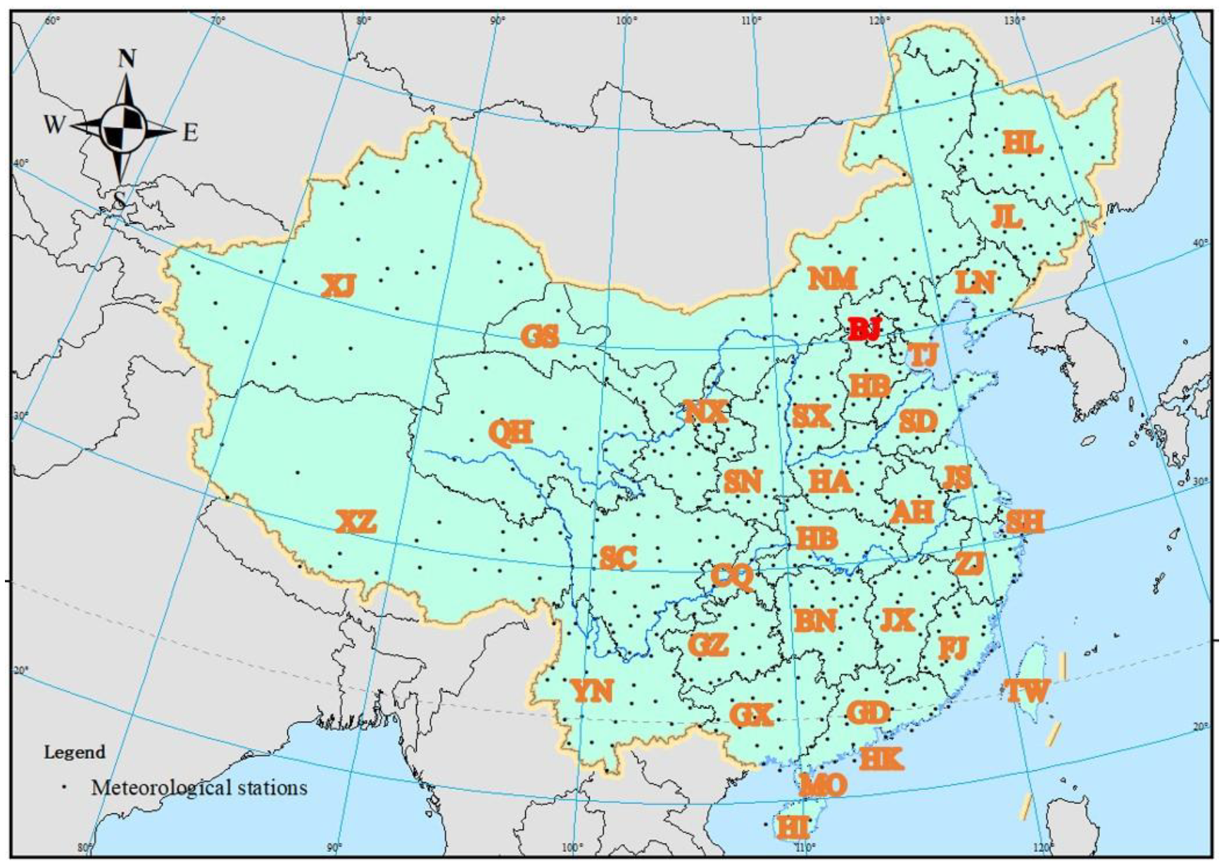
2.1. Study Area and Climate Dataset

Located in the east of Asia, China is the third largest country in the world in land area, with an estimated land area of 9.6 million square kilometers and a population of over 1.4 billion. Its terrain is generally high in the West and low in the East. Most of the areas belong to temperate and subtropical monsoon climate, with rich and diverse climate types and geographical landscape. The issues surrounding in China are severe partially because it has uneven spatial and temporal distribution of water resources. The precipitation generally decreases from the southeast coast to northwest inland. The cultivated land in the Yangtze River Basin and south of the Yangtze River only accounts for 36% of China’s total, while water resources account for 80% of China’s total. In the Yellow River, Huaihe River and Haihe River basins, water resources only account for 8% of China’s total, while arable land accounts for 40% of China’s total. The annual and interannual variation of precipitation and runoff is large. These characteristics of water resources cause frequent floods and droughts in China, and agricultural production is also relatively unstable.
In the present study, a total of four spatial scales were considered: continental, regional, provincial, and local. The continental scale was equivalent to the national scale, which covered mainland China. At the regional scale, the study area has been divided into 7 sub-regions by the following geographic locations: North Eastern Region (NER), North China Region (NCR), East China Region (ECR), South China Region (SCR), Central China Region (CCR), North Western Region (NWR), and South Western Region (SWR). A large portion of the water resources activities in China are governed by provincial water management authorities, so the provincial scale was also considered. The local scale considered the stations that have sufficient quality data.
The daily climatic data employed in this study included daily Hm, SD, Tmax, Tmin, and Uw at 10 m height (U10). The data of U10 has been converted to U2 (Uw at 2 m height) using the transformation formula provided by Allen et al. [32]. The data were primarily obtained from the China Meteorological Administration. The quality of the dataset has been carefully controlled, and the dataset has been widely used in previous studies [9,24,28]. There were 665 stations in the original dataset, but 129 of the stations were excluded because they had extensive missing data; finally, 536 stations were selected. The study area and selected meteorological stations are presented in Figure 1. The subregions, the provinces, and the corresponding numbers of meteorological stations are provided in Table 1.

2.2. ET0 Calculation
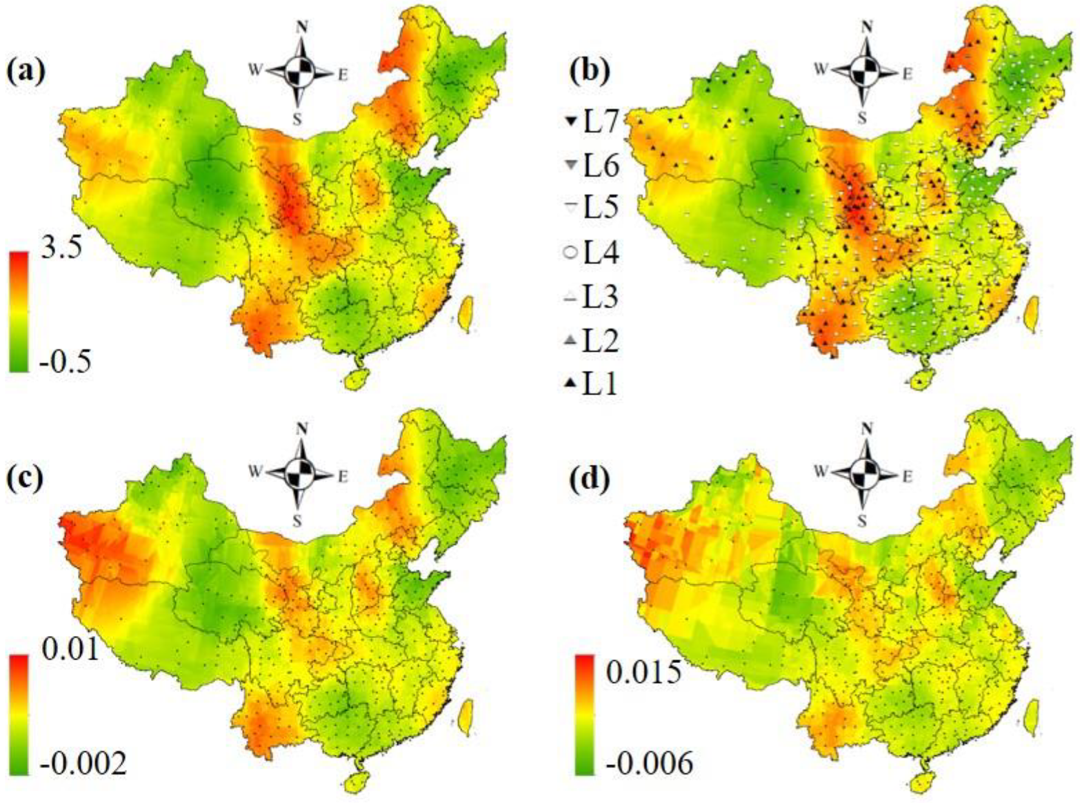
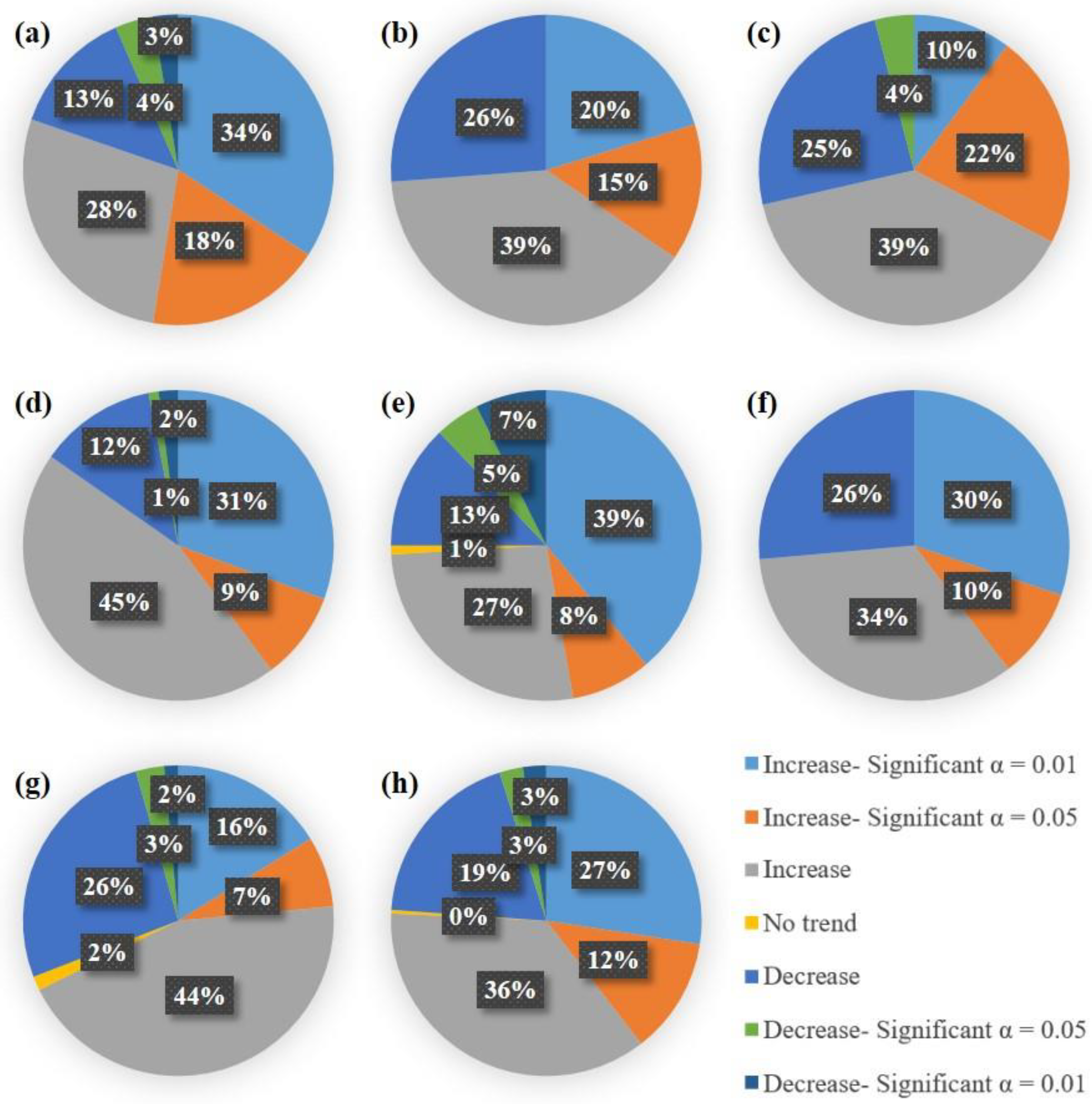
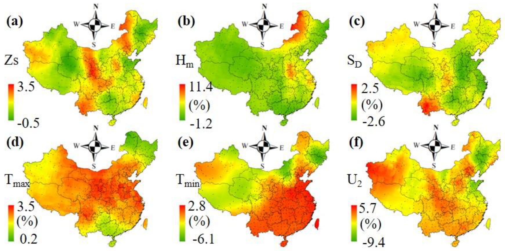
The present study employed the FAO Penman–Monteith (P–M) equation to calculate the daily ET0. In March 1990, the Food and Agriculture Organization of the United Nations (FAO) recommended the use of this formula to calculate ET0 at the international symposium on crop evapotranspiration calculation methods held in Rome, Italy [19]. The formula is the most widely used method to calculate ET0 in the world. The P–M formula, physically based on both the energy balance and aerodynamics, does not need a special regional calibration function, and it can calculate ET0 by using general meteorological data, which has high practical value and accuracy [33]. The equation can be written as
E T 0 = 0.408 Δ ( R n G ) + γ [ 900 / ( T + 273 ) ] U 2 ( e s e a ) Δ + γ ( 1 + 0.34 U 2 )
where E T 0 is the reference evapotranspiration (mm day–1); Δ is the slope vapor pressure curve (kPa °C−1); R n is the net radiation at the crop surface (MJ m−2 day−1); G is the soil heat flux density (MJ m−2 day−1); γ is the psychrometric constant (kPa °C−1); T is the mean daily air temperature at 2 m height (°C); U 2 is the Uw at the 2m height (m/s); e s is the saturation vapor pressure (kPa); e a is the actual vapor pressure (kPa). The intermediate variables can be calculated from daily Hm, SD, Tmax, Tmin, and U2, following the equations provided in the FAO56 report [32].

2.3. Trend Analysis

The present study used the Mann–Kendall trend test approach to detect significant trends in ET0 and its contributing climatic variables. The Mann–Kendall (MK) test [34,35,36] is a nonparametric (distribution-free) test, and it was employed in this study because it has been widely used in assessing whether there is a monotonic upward or downward trend of hydrological variables over time [27,37]. Its superiority exists in the ability of detecting the significance of the long time-series trend, no matter the sample series follow a certain type of distribution [38]. In the MK test, S is a statistical value used to determine whether values obtained later in time tend to be larger than values obtained earlier, as:
S = i = 2 n j = 1 i = 1 s i g n ( x i x j ) ,
where n is the number of observations and s i g n ( x i x j ) can be expressed as:
s i g n ( x i x j ) = { - 1   if   ( x i x j ) < 0   0         if   ( x i x j ) = 0 1         if   ( x i x j ) > 0 } ,
The variance of S can be computed as follows:
V a r ( S ) = n ( n 1 ) ( 2 n + 5 ) k 1 l t k ( t k 1 ) ( 2 t k + 5 ) 18 ,
where l is the number of tied groups, and tk is the number of observations in the tth group.
The MK test statistic, ZS, can be expressed as:
Z S = { S + 1 V a r ( S )   if   S < 0 0     if   S = 0 S 1 V a r ( S )   if   S > 0 } ,
Positive values of ZS indicate that the variables of interest tend to increase with time, and negative values of ZS indicate that the variables of interest tend to decrease with time. The null hypothesis of no trend is rejected when |ZS| > 1.96 at the α = 0.05 level and |ZS| > 2.576 at the α = 0.01 level.
To estimate the slope of the linear trend, the time series of a variable (e.g., ET0) were fitted into a linear regression equation, such as
E T 0 = T L t + b
where TL is slope of the liner trend.
The slope of trend can also be estimated using a nonparametric procedure developed by Sen [39]. In the procedures, the slopes of N pairs of observations are first estimated by
Q i = x j x k j k   for   i = 1 , , N
where xj is the value at time j, while xk is the value at time k (j > k). Since there is only one datum in each time period in the present study, N can be computed as N = n ( n 1 ) 2 and n is the number of time steps. The values of these slopes are then ranked from smallest to largest, and the median value is known as the Sen’s estimator of slope. When N is odd, Sen’s estimator of slope is Q ( N + 1 ) / 2 ; when N is even, Sen’s estimator of slope is Q N / 2 + Q ( N + 2 ) / 2 2 .
To verify whether the median slope is statistically different from zero, the confidence interval for Sen’s estimator of slope, for a given level of significance α, should be computed [34]. The confidence interval can be computed as follows:
C α = Z 1 α / 2 V a r ( S )
where Var(S) is computed by (4), and Z1−α/2 is obtained from the standard normal distribution table. The approximate normal theoretical lower and upper confidence limit are respectively the M1th largest and the (M2+1)th largest of value of Q. M1 and M2 are defined by
M 1 = N C α 2 ; M 2 = N + C α 2
the Sen’s estimator of slope is statistically different from zero if the two limits Q(M1) and Q(M2) have the same sign.

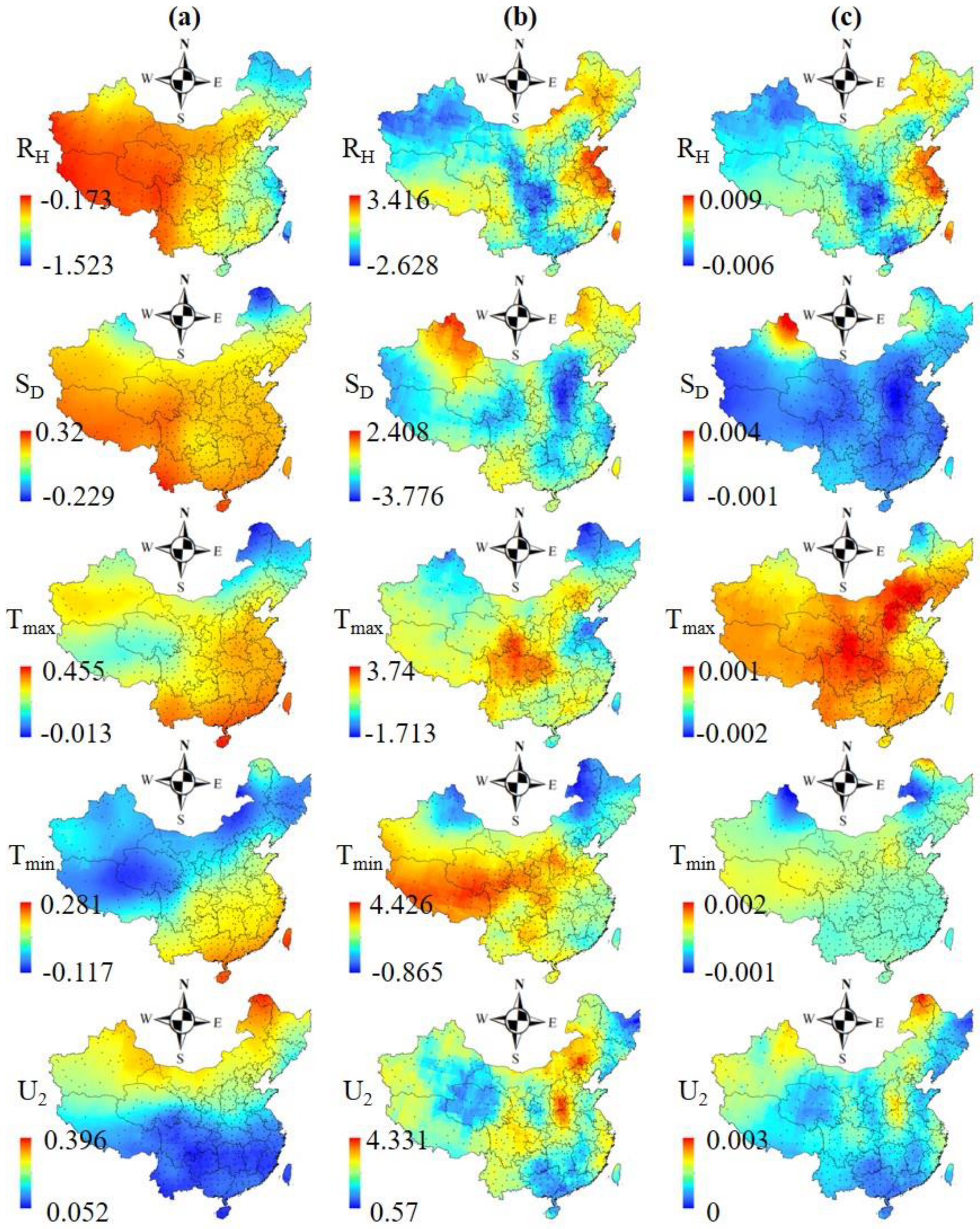
2.4. Sensitivity Coefficient and Contribution Rate

The sensitivity coefficient, Sti, that quantifies the sensitivity of ET0 to a climatic variable, ci, can be expressed as [27]:
S t i = E T 0 c i c i E T 0
If Sti > 0, ET0 and ci will increase or decrease simultaneously, otherwise, they have a reverse relation. The larger the |Sti|, the greater the effect of a climatic variable has on ET0 variation. The sensitivity coefficient method is more convenient and accurate compared to other sensitivity analysis approaches [40], and it has been widely used in hydro-meteorological study.
The contribution rate of ci, Cbi, to ET0 variation, can be expressed as [27]:
C b i = S t i n × T d i | A c i | × 100 %
where n is the number of observations, Tdi is the trend of the variable ci, and | A c i | is the absolute value of the averaged ci. If the Cbi is positive (negative), it denotes the variable had a positive (negative) contribution to ET0 variation. The method can clearly reveal how the climatic variables contribute to ET0.

3. Results

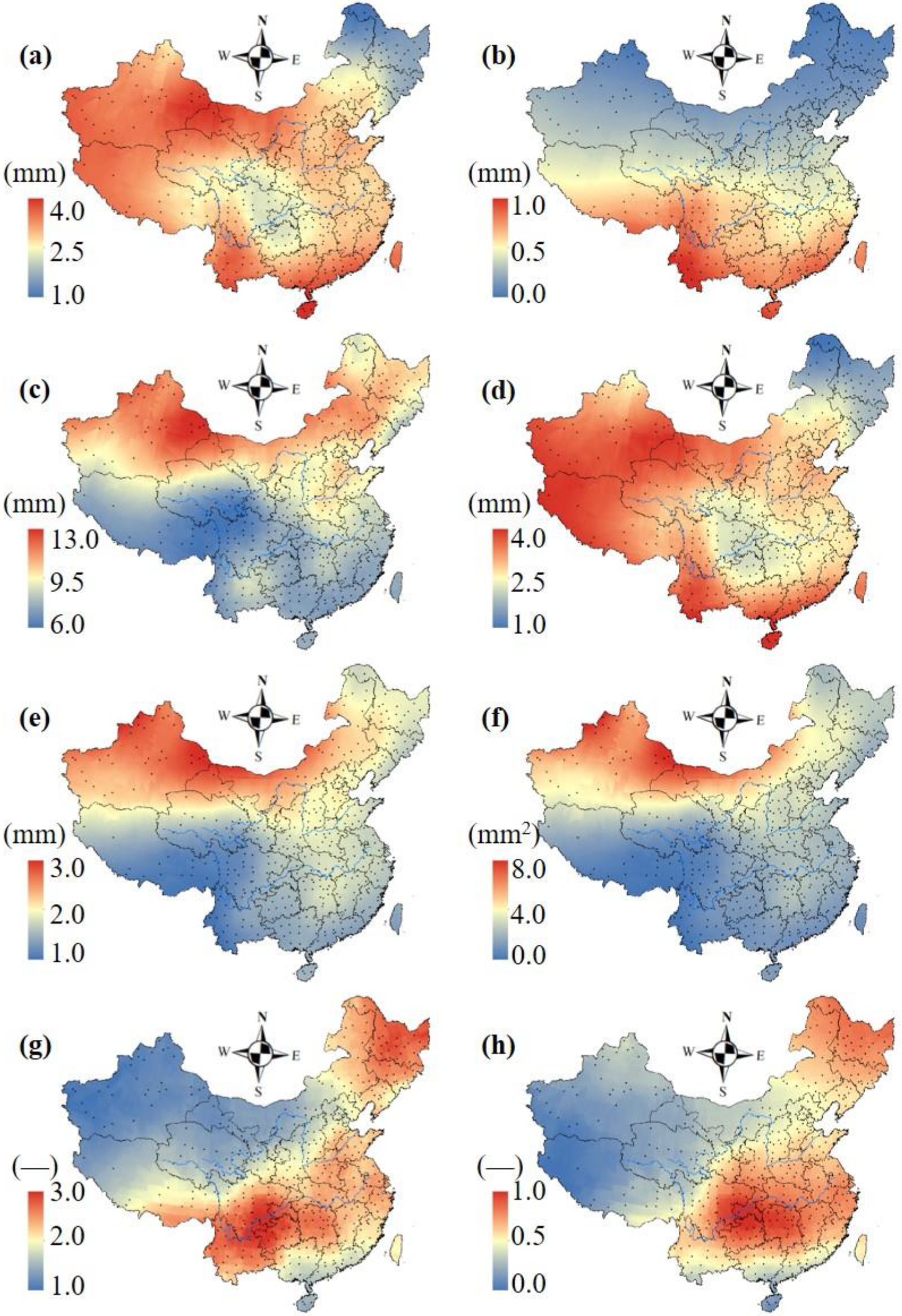
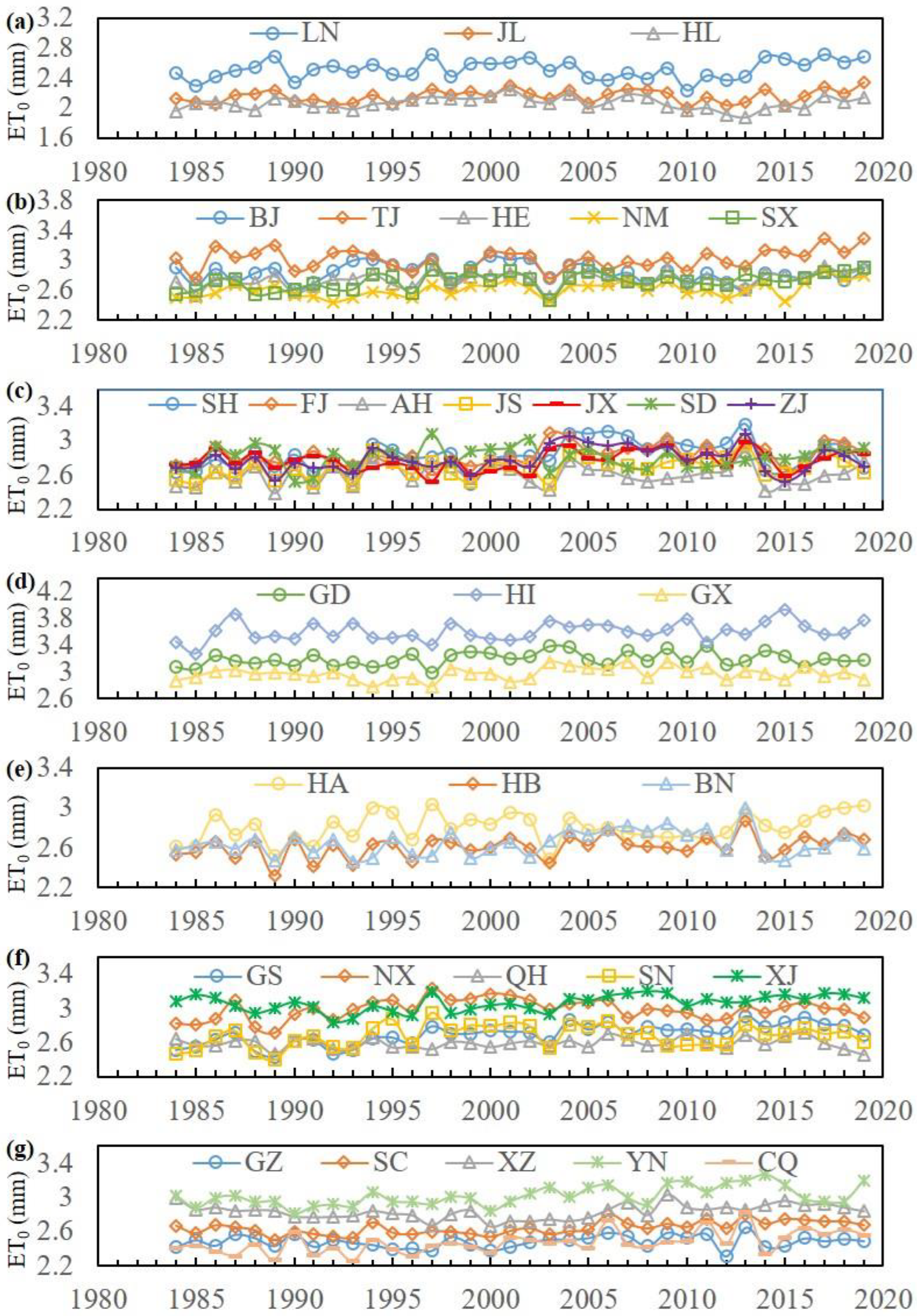
3.1. Spatiotemporal Variation of ET0

Figure 2 shows the descriptive statistics of daily ET0 at the 536 stations. The spatial distribution plots, which were obtained by interpolating the results using the Kriging interpolation approach, are provided primarily for the purpose of visualization. The mean daily ET0 ranged from around 1 mm (mainly in the northeast) to around 4 mm (such as in the southern edge). The minimum daily ET0 in the northern part was close to 0 mm, partially because the winter temperature in the north was quite low. The minimum daily ET0 in the southern part was around 1 mm. Although the temperature increased from north to south, the maximum daily ET0 showed a reverse trend, which may partially be attributed to the higher U2 in the northern part, and revealed that ET0 is the combined result of various climatic variables. The median values were close to the mean values. Generally, the standard deviation and variance decreased from north to south, and the kurtosis and skewness increased from northeast to southwest.
The results of the M–K trend analysis are shown in Figure 3. ET0 increased at 406 of the 536 stations (75.7%), with the trends being significant at 65 stations at the 5% significance level, and 147 at the 1% significance level. ET0 decreased at 128 out of the 536 stations (23.9%), with the trends being significant at 13 stations at the 5% significance level, and 13 at the 1% significance level. In general, most of the stations exhibited an increasing ET0, and the stations showing significant increasing trends were primarily located in NM, NX, GS, SC, CQ, and YN. The averaged slope calculated using Sen’s method and linear trend method were 0.0033 and 0.0034, respectively. Therefore, the annual ET0 at the continental scale increased by approximately 12 mm/decade in China.

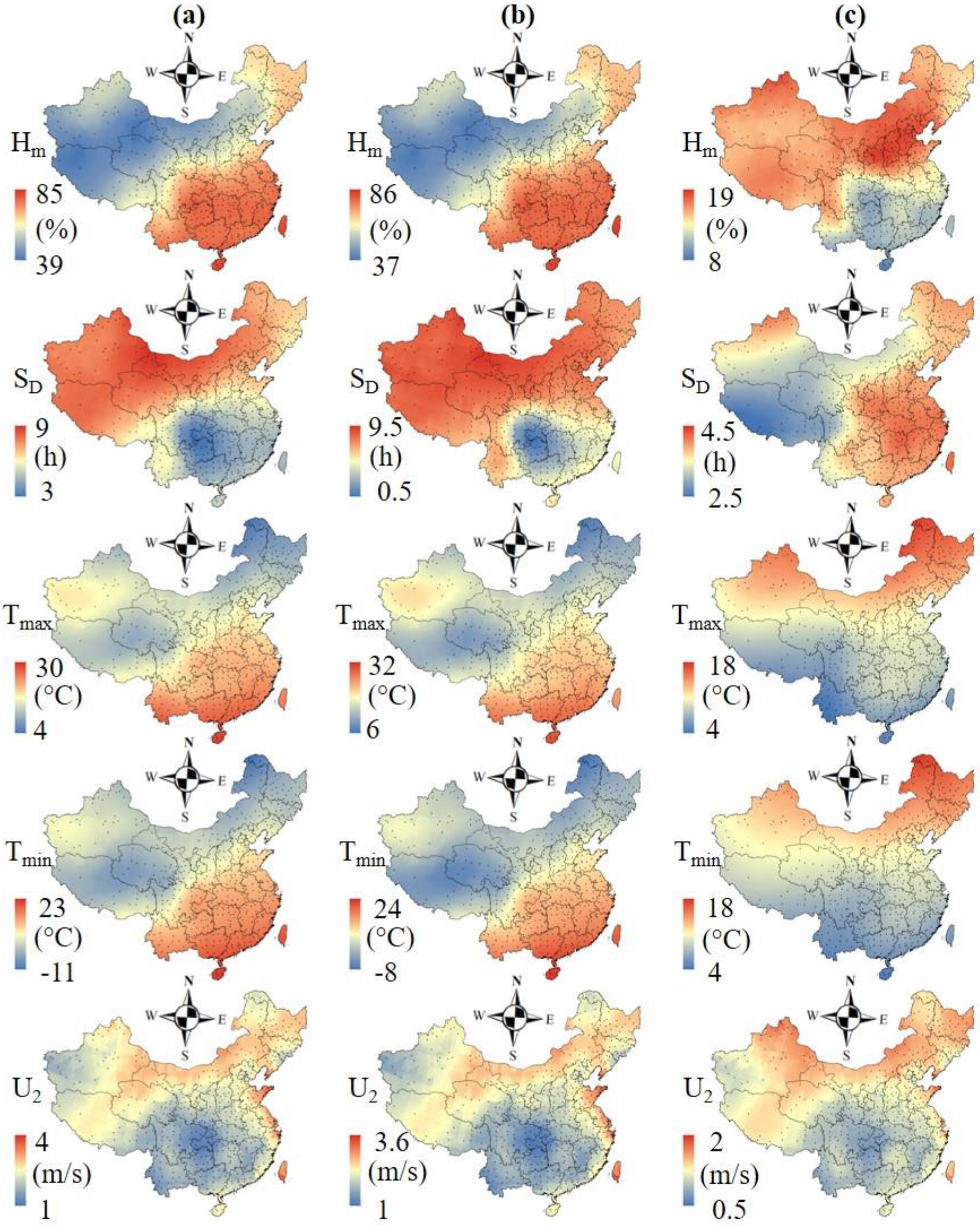
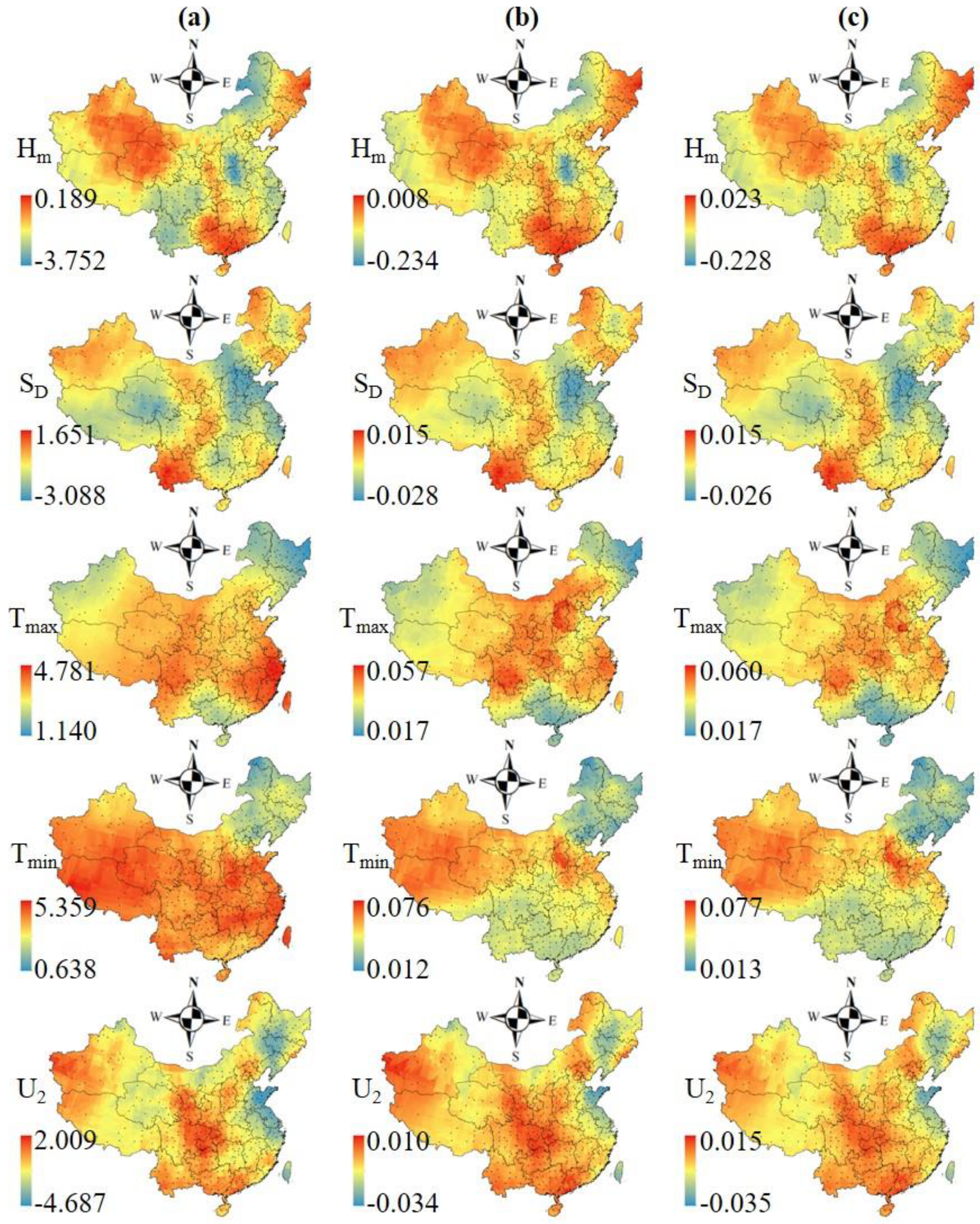
3.2. Spatiotemporal Variation of Climatic Factors

The descriptive statistics of the climatic variables were shown in Figure 4. Based on the mean data, Hm increased from the northwest (less than 40%) to the southeast (more than 80%); SD decreased from west (as high as 9 h) to east (as low as 3 h); Tmax increased from north (lower than 5 °C) to south (close to 30 °C); Tmin also increased from north (lower than −10 °C) to south (higher than 20 °C); and U2 decreased from north (close to 4 m/s) to south (as low as 1 m/s). The median values were close to the mean values. The standard deviations ranged from around 19% in the northwest to around 8% in southeast. Conversely, the standard deviations for SD increased from the northwest (approximately 4.5 h) to the southeast (approximately 2.5 h). The standard deviations for Tmax, Tmin, and U2 all decreased from north to east. These standard deviations can quantify how accurate it was to estimate climatic variables at a smaller spatial scale using characteristics at a larger spatial scale.
Figure 5 shows the results of trend analysis for the climatic variables. Hm decreased at 443 of the 536 stations (82.6%), and the averaged slopes calculated using Sen’s method and linear trend method were −0.089 and −0.086, respectively. The majority of the stations (67.2%) exhibited decreasing SD, with an average trend slope of −0.006 (Sen’s = −0.006; and linear = −0.006). Most of the stations showed increasing Tmax (532 stations; 99.3%), and the averaged slope was 0.039 (Sen’s = 0.040; and linear = 0.039). Similarly, most of the stations (512 stations; 95.5%) had an increasing Tmin with the averaged slope being 0.042 (Sen’s = 0.042; and linear = 0.042). The U2 showed an overall decreasing trend, as 324 stations (60.4%) had a declining U2, and the averaged Sen’s slope and linear slope were −0.007 and −0.005, respectively.

4. Discussion

4.1. Variability of ET0 at Various Spatial Scales

The descriptive statistics of daily ET0 for each station (at the local scale) have been presented in Figure 2 and the mean values were averaged to obtain the mean ET0 at the provincial, regional, and continental scales. This averaging approach was used for upscaling, instead of other approaches based on interpolations, to avoid the large uncertainties caused by spatial interpolations. At the continental scale, the daily ET0 across China for 1984–2019 was 2.72 mm/day. However, the standard deviation of the mean daily ET0 at different stations was 0.40 mm/day, which was quite high, indicating that the ET0 characteristics found at the continental scale cannot provide meaningful insight for local water management. Wang et al. [26] investigated the spatiotemporal variability of ET0 during 1961–2013 using a gridded dataset and also revealed that the ET0 in China differed significantly. Thus, the ET0 variation characteristics across different spatial scales should be investigated.
At the regional scale, the averaged daily ET0 was the highest in South China (SCR), which was 3.25 mm/day, followed by NWR (2.80 mm/day), NCR (2.78 mm/day), ECR (2.76 mm/day), SWR (2.69 mm/day), and CCR (2.68 mm/day). The averaged ET0 was the lowest in North East (NER), which was 2.24 mm/day.
Figure 6 illustrates the time series of annual mean daily ET0 at the provincial scale. In the area NER, province LN generally had the highest ET0 (mean ET0 =2.51 mm/d), while HL had the lowest ET0 (mean ET0 = 2.06 mm/d). Province TJ had the highest ET0 (mean ET0 = 3.01 mm/d) in the subregion NCR, and NM had the lowest ET0 (mean ET0 = 2.61 mm/d). In ECR, the ET0 was the highest in province SH (mean ET0 = 2.83 mm/d) and the lowest in AH (mean ET0 = 2.60 mm/d). In the subregion SCR, ET0 ranged from 2.96 mm/d in GX to 3.60 mm/d in HI. In the subregion CCR, the difference in ET0 was relatively small, with HA being the province with the highest ET0 (mean ET0 = 2.80 mm/d) and HB being the province with the lowest ET0 (mean ET0 = 2.61 mm/d). The province that had the maximum mean ET0 in the subregion NWR was XJ (mean ET0 =3.06 mm/d), and the one that had the minimum mean ET0 was QH. In the subregion SWR, the mean ET0 ranged from 2.47mm/d in province CQ to 3.02 mm/d in YN. In some areas, such as SCR, the differences at different locations were relatively small, and thus, it is reasonable to estimate ET0 characteristics at a smaller spatial scale using ET0 characteristics at a larger spatial scale. However, most of the regions exhibited significant differences of ET0 at different locations; thus, the regional observations cannot well represent the provincial characteristics.
The trends in ET0 variations at the local scale have been presented in Figure 3, and the trends at the provincial and regional scales can be analyzed based upon these trends. The statistics regarding the trends in ET0 at the regional scale are summarized in Figure 7. In the subregion NCR, 34% of the stations showed a trend of “increase-significant α = 0.01”, followed by “increase” (28%) and “increase-significant α = 0.05” (18%). In the area ECR, 39% of the stations showed a trend of “increase”, followed by “decrease” (26%) and “increase-significant α = 0.01” (20%). 39% of the stations in the subregion SCR showed a trend of ” increase”, while 25% showed a trend of “decrease” and 22% showed a trend of “increase-significant α = 0.05”. In the area SWR, a large portion of the stations showed a trend of “increase” (45%) and “increase-significant α = 0.01” (31%), and 12% of the stations showed a trend of “decrease”. There were 39%, 27%, and 13% of the stations in the subregion NWR that showed a trend of “increase-significant α = 0.01”, “increase”, and “decrease” (13%), respectively. The majority of the stations in CCR showed an increasing trend (34% “increase” and 30% “increase-significant α = 0.01” (30%)”, and there were also 26% that showed the “decrease” trend. In the subregion NER, most of the stations (44%) showed a trend of “increase”; however, there were also 26% of the stations showed a trend of “decrease” (26%), exhibiting a significant diverse; the portion of stations that showed a trend of “increase-significant α = 0.01” was 16%. At the continental scale, the annual ET0 increased by approximately 12 mm/decade for 1984–2019. Most of the stations showed increasing trends, with 36% of the stations exhibiting a trend of “increase” and 27% exhibiting “increase-significant α = 0.01”(27%); however, there were also 19% of the stations that showed a trend of “decrease”. Zhang et al. [31] studied evapotranspiration (ET) in China for 1948–2018 and found that the ET in most regions (covered by 89.5% pixels) showed increasing trends, which was close to the current observation. Zhang et al. [31] reported that the fluctuation of ET was relatively larger in the north and west, and relatively weaker in the south and east. The present study found the same characteristic, but it reported the standard deviations and variances of ET0 variations at each station to quantitatively describe the fluctuations (Figure 2).

4.2. Variability of Climatic Variables at Various Spatial Scales

The statistics at the regional and continental (national) scales are illustrated in Figure 8, in which the trends and M–K Zs values are also indicated. The lower lines of the boxes indicated the lower quartiles, which were the medians of the lower half of the datasets, the medium lines correspond to the middle values of the entire datasets, and the upper lines indicate the upper quartiles, which were the medians of the upper half of the datasets. These lines of boxes can also provide insight for the variability of climatic variables at the provincial scale.
As can be seen, the Hm in ECR, SCR, and CCR was relatively higher, whereas that in NCR and NWR was relatively lower. All of the subregions showed decreasing trends in Hm, with NCR having the most significant trend (Zs = −2.39) and SCR having the least significant trend rate (Zs = −0.78). The subregions NCR, NWR, and NER had relatively greater values of SD than the other subregions. SD was declining in all of the areas, and the absolute value of Zs was the largest in NCR (Zs = −1.52) and smallest in SWR (Zs = −0.34). Yin et al. [15] has studied the potential evapotranspiration (PET) and its determining factors in China for 1971–2008 and has also found a decreasing trend of SD. Tmax in SCR, CCR, and ECR was relatively higher than others in NCR and NER. All of the areas showed increasing trends, with the Zs values ranging from 2.18 in NER to 4.13 in ECR. Similarly, Tmin was also increasing in all of the subregions. Tmin in ECR, SCR, and NER was relatively higher, whereas that in NCR and NWR was relatively lower. The Zs values for Tmin ranged from 2.16 in NER to 4.59 in CCR. In contrast to Tmax and Tmin, U2 showed a decreasing trend, with SCR having the most significant trend rate (Zs = −0.04) and ECR having the least significant (Zs = −2.68). The subregions with relatively high U2 included NCR, ECR, and NER, and those subregions with low U2 included SWR, SCR, and CCR. Yin et al. [15] has also found that U2 showed a decreasing trend. In summary, the results at the continental scale can well represent the trend directions at the regional scale. In some regions, the findings at the regional scale can satisfactorily represent the characteristics at the provincial and local scales, such as Hm in SCR and Tmax in SWR. However, in most regions, both the statistics and trend rates exhibited substantial variations across spatial scales, such as SD in ECR and Tmin in NER.

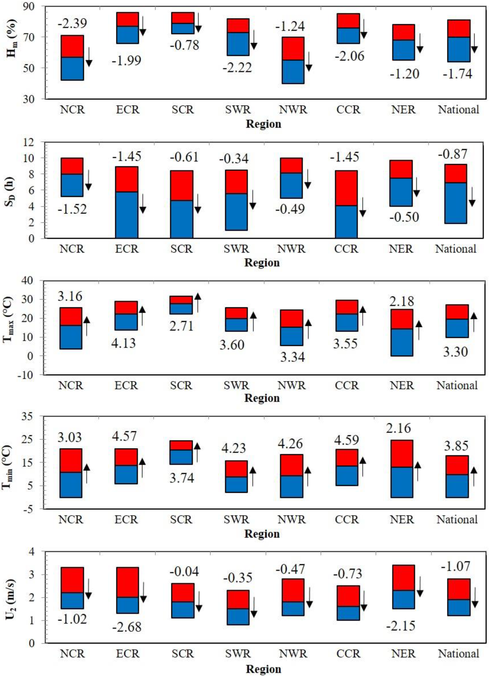
4.3. Sensitivity and Contribution

The variations in ET0 are the combined effects of the climatic variables; thus, it is important to quantify the sensitivity of ET0 to these factors for a better understanding of the driving mechanisms. The mean values of the sensitivity coefficients, the corresponding trends (Zs values), and trend rates (Sen’s slope) at the local scale are presented in Figure 9.
Figure 9 shows that ET0 at most stations was negatively correlated to the variations in Hm, while ET0 at most stations was positively correlated to the variations in the other climatic variables. At the continental scale, ET0 was most sensitive to Hm (average St = −0.66), followed by Tmax (St = 0.29), SD (St = 0.18), U2 (St = 0.16), and Tmin (St = 0.07). Yin et al. (2010) also revealed that Hm was the most sensitive variable for PET.
Consistent with the observations of Fan and Thomas [29], who studied ET0 in China for the period of 1960–2011, the importance of the climatic variables to ET0 were not stable. Most of the stations showed increasing trends in St for Hm (56.16%), with a Zs value of 0.37 and a slope of 0.00092 at the continental scale. Fan and Thomas [29] has also found that the importance of Hm increased in China. In terms of SD, 69.78% of the stations showed decreasing trends, and the Zs value and slope at the continental scale were −1.15 and −0.00027, respectively. Liu et al. [25] found that the sensitivity of Tmax exhibited declining trends while that of Tmin showed increasing trends in China for 1960–2007. However, based on the present study, which covered a longer time period, the majority of the stations showed increasing trends in St for Tmax (72.95%) and Tmin (87.31). The Zs values at the continental scale corresponding to Tmax and Tmin were 1.25 and 2.16, respectively, and the slopes at the continental scale were 0.00040 and 0.00032, respectively. Interestingly, 90.49% of the stations showed increasing trends in St for U2, implying that U2 was becoming more important in affecting ET0. Liu et al. [25] also found that the sensitivity of U2 showed an increasing trend in China for 1960–2007. The Zs value and slope at the continental scale corresponding to U2 was 2.38 and 0.00106, respectively.
The contribution of each climatic variable to the variation in ET0 was quantified in Figure 10, in which the spatial distribution of Zs for ET0 was also shown for a better interpretation of the climatic effects. As can be seen from Figure 10, the variations in Hm increased ET0 at most of the stations (441 stations; 82.28%), and the Cb at the continental scale was 2.83%. Similarly, the variations in Tmax and Tmin increase ET0 at 526 stations (98.13%) and 370 stations (69.03%), respectively, and the Cb values at the continental scale were 2.32% and 0.07%, respectively. However, for most stations, the variations in SD and U2 decreased ET0 at most of the stations (354 stations and 302 stations, respectively), and the Cb values at the continental scale were −0.67% and −0.70%, respectively. Yao et al. [30] studied the PET across China for 1982–2010 and found that PET was mostly attributed to the incident solar radiation, followed by pressure deficit, air temperature, and wind speed, which were close to the current observations. Ullah et al. [40] and Hina et al. [41] investigated the climatic variables related to drought and possible cycles over Pakistan. The analysis of atmospheric circulation patterns revealed that large-scale changes in wind speed, air temperature, relative humidity, and so on are the likely drivers of droughts in the region, which also confirmed the current observations were reasonable. Sein et al. [42] assessed the spatiotemporal variation of summer monsoon precipitation and its potential drivers in Myanmar and found that the spatial trends for monthly and seasonal precipitation vary from station to station and region to region due to a fluctuated shift of climatic dynamics, which demonstrated the precipitation and ET0 variability is associated with regional scale atmospheric circulation and some climatic variables. Based on the values of Cb obtained in this study using the latest dataset, it can be concluded that the variations in ET0 were mostly attributed to Hm, Tmax, U2, SD, and Tmin.

5. Conclusions

Daily ET0 at 536 meteorological stations in China for the period 1984–2019 were calculated, the trends in ET0 and its contributing climatic variables were analyzed, and the sensitivity of ET0 to the meteorological variables and the contribution rates of the meteorological variables to the ET0 variations were discussed. A key novelty of this study was that the variability of ET0 and the contributing meteorological variables at various spatial scales were investigated. Generally, ET0 decreased from south to north. The core of high ET0 was primarily located near the southern edge. Generally, the standard deviation and variance decreased from north to south, and the kurtosis and skewness increased from northeast to southwest. The ET0 increased at 406 of the 536 stations, and the averaged slope showed that the annual ET0 increased by approximately 12 mm/decade in China. Most of the stations showed decreasing trends in Hm (Zs = −1.74), SD (Zs = −0.87), and U2 (Zs = −1.07) and increasing trends in Tmax (Zs = 3.30) and Tmin (Zs = 3.85).
ET0 was negatively correlated to Hm, and the average sensitivity coefficient was −0.66. In terms of positively correlated variables, ET0 was most sensitive to Tmax (St = 0.29), followed by SD (St = 0.18), U2 (St = 0.16), and Tmin (St = 0.07). The St for Hm at most stations (56.16%) were increasing while the SD at most stations (69.78%) were decreasing. The majority of the stations showed increasing trends in St for Tmax (72.95%) and Tmin (87.31%). Interestingly, 90.49% of the stations showed increasing trends in St for U2, implying that U2 was becoming more important in affecting ET0. The variations in Hm, Tmax, and Tmin increased the ET0 at most of the stations (the mean contribution rate was 2.83%, 2.32%, and 0.07%, respectively). However, at most stations, the variations in SD and U2 decreased ET0, and the mean Cb values were −0.67% and −0.70%, respectively.
The present study reported an analysis of trends in ET0 and its contributing climatic variables at four different spatial scales. Compared to analyses of a single or two spatial scales, the present analysis can better illustrate the variation trends and aid in future studies in water resources, agriculture, and hydrology in China. This study is also meaningful for modeling of hydrodynamics and water quality in inland and coastal water: first, the data can be directly used as inputs of the models; and second, the studied ET0 characteristics can provide a better understanding of the mechanics and reasons for the variations in hydrodynamics and water quality. The present study found that the variations in ET0, climatic variables, sensitivity coefficients, and contribution rates were significant at some stations, so it is important to regularly update the corresponding forecasts. The significant variations also emphasize that it is important to develop sustainable water resources management and water-saving irrigation techniques under the condition of climate change. This study used the averaging approach for upscaling, it deserves a separate study to perform other upscaling techniques to study ET0 characteristics at different scales.

Author Contributions

Funding acquisition, methodology, project administration, writing original draft, X.Y.; Funding acquisition, investigation, writing review and editing, A.M.; Methodology, visualization, R.A.; Writing review and editing, J.L.; Writing review and editing, X.C. All authors have read and agreed to the published version of the manuscript.

Funding

This research was funded by the Fundamental Research Funds for the Central Universities (China; DUT20RC(3)096), and Natural Sciences and Engineering Research Council of Canada (NSERC Discovery Grants).

Institutional Review Board Statement

Not applicable.

Informed Consent Statement

Not applicable.

Data Availability Statement

The data supporting reported results can be found from the China Meteorological Administration (http://data.cma.cn (accessed on 10 August 2022)).

Acknowledgments

The research is supported by the Fundamental Research Fund s for the Central Universities (China; DUT20RC(3)096). We would like to thank the China Meteorological Administration for providing the daily meteorological data.

Conflicts of Interest

The authors declare no conflict of interest.

List of Acronyms and Symbols

ET0reference evapotranspiration;
Hmhumidity;
SDsunshine duration;
Tmaxmaximum air temperature;
Tminminimum air temperature;
Uwwind speed;
U2Uw at 2 m height;
U10Uw at 10 m height;

References

  1. Luo, Y.; Chang, X.; Peng, S.; Khan, S.; Wang, W.; Zheng, Q.; Cai, X. Short-term forecasting of daily reference evapotranspiration using the Hargreaves–Samani model and temperature forecasts. Agric. Water Manag. 2014, 136, 42–51. [Google Scholar] [CrossRef]
  2. Luo, Y.; Traore, S.; Lyu, X.; Wang, W.; Wang, Y.; Xie, Y.; Jiao, X.; Fipps, G. Medium Range Daily Reference Evapotranspiration Forecasting by Using ANN and Public Weather Forecasts. Water Resour. Manag. 2015, 29, 3863–3876. [Google Scholar] [CrossRef]
  3. Aouissi, J.; Benabdallah, S.; Chabaâne, Z.L.; Cudennec, C. Evaluation of potential evapotranspiration assessment methods for hydrological modelling with SWAT—Application in data-scarce rural Tunisia. Agric. Water Manag. 2016, 174, 39–51. [Google Scholar] [CrossRef]
  4. Yang, Y.; Cui, Y.; Luo, Y.; Lyu, X.; Traore, S.; Khan, S.; Wang, W. Short-term forecasting of daily reference evapotranspiration using the Penman-Monteith model and public weather forecasts. Agric. Water Manag. 2016, 177, 329–339. [Google Scholar] [CrossRef]
  5. Yang, Y.; Cui, Y.; Bai, K.; Luo, T.; Dai, J.; Wang, W.; Luo, Y. Short-term forecasting of daily reference evapotranspiration using the reduced-set Penman-Monteith model and public weather forecasts. Agric. Water Manag. 2019, 211, 70–80. [Google Scholar] [CrossRef]
  6. Chen, Z.; Zhu, Z.; Jiang, H.; Sun, S. Estimating daily reference evapotranspiration based on limited meteorological data using deep learning and classical machine learning methods. J. Hydrol. 2020, 591, 125286. [Google Scholar] [CrossRef]
  7. Yan, X.; Mohammadian, A. Forecasting daily reference evapotranspiration for Canada using the Penman–Monteith model and statistically downscaled global climate model projections. Alex. Eng. J. 2020, 59, 883–891. [Google Scholar] [CrossRef]
  8. Yan, X.; Mohammadian, A. Estimating future daily pan evaporation for Qatar using the Hargreaves model and statistically downscaled global climate model projections under RCP climate change scenarios. Arab. J. Geosci. 2020, 13, 1–15. [Google Scholar] [CrossRef]
  9. Yin, J.; Deng, Z.; Ines, A.V.; Wu, J.; Rasu, E. Forecast of short-term daily reference evapotranspiration under limited meteorological variables using a hybrid bi-directional long short-term memory model (Bi-LSTM). Agric. Water Manag. 2020, 242, 106386. [Google Scholar] [CrossRef]
  10. Iyakaremye, V.; Zeng, G.; Yang, X.; Zhang, G.; Ullah, I.; Gahigi, A.; Vuguziga, F.; Asfaw, T.G.; Ayugi, B. Increased high-temperature extremes and associated population exposure in Africa by the mid-21st century. Sci. Total Environ. 2021, 790, 148162. [Google Scholar] [CrossRef] [PubMed]
  11. Ullah, I.; Saleem, F.; Iyakaremye, V.; Yin, J.; Ma, X.; Syed, S.; Hina, S.; Asfaw, T.G.; Omer, A. Projected Changes in Socioeconomic Exposure to Heatwaves in South Asia Under Changing Climate. Earth’s Future 2022, 10, e2021EF002240. [Google Scholar] [CrossRef]
  12. Traore, S.; Luo, Y.; Fipps, G. Deployment of artificial neural network for short-term forecasting of evapotranspiration using public weather forecast restricted messages. Agric. Water Manag. 2016, 163, 363–379. [Google Scholar] [CrossRef]
  13. Althoff, D.; Dias SH, B.; Filgueiras, R.; Rodrigues, L.N. ETo-Brazil: A Daily Gridded Reference Evapotranspiration Data Set for Brazil (2000–2018). Water Resour. Res. 2020, 56, e2020WR027562. [Google Scholar] [CrossRef]
  14. Mohammadi, B.; Mehdizadeh, S. Modeling daily reference evapotranspiration via a novel approach based on support vector regression coupled with whale optimization algorithm. Agric. Water Manag. 2020, 237, 106145. [Google Scholar] [CrossRef]
  15. Yin, Y.; Wu, S.; Dai, E. Determining factors in potential evapotranspiration changes over China in the period 1971–2008. Chin. Sci. Bull. 2010, 55, 3329–3337. [Google Scholar] [CrossRef]
  16. Ahmadi, F.; Mehdizadeh, S.; Mohammadi, B.; Pham, Q.B.; Doan, T.N.C.; Vo, N.D. Application of an artificial intelligence technique enhanced with intelligent water drops for monthly reference evapotranspiration estimation. Agric. Water Manag. 2021, 244, 106622. [Google Scholar] [CrossRef]
  17. Yan, S.; Wu, L.; Fan, J.; Zhang, F.; Zou, Y.; Wu, Y. A novel hybrid WOA-XGB model for estimating daily reference evapotranspiration using local and external meteorological data: Applications in arid and humid regions of China. Agric. Water Manag. 2021, 244, 106594. [Google Scholar] [CrossRef]
  18. Tang, B.; Tong, L.; Kang, S.; Zhang, L. Impacts of climate variability on reference evapotranspiration over 58 years in the Haihe river basin of north China. Agric. Water Manag. 2011, 98, 1660–1670. [Google Scholar] [CrossRef]
  19. Roy, D.K.; Barzegar, R.; Quilty, J.; Adamowski, J. Using ensembles of adaptive neuro-fuzzy inference system and optimization algorithms to predict reference evapotranspiration in subtropical climatic zones. J. Hydrol. 2020, 591, 125509. [Google Scholar] [CrossRef]
  20. Lawrimore, J.H.; Peterson, T.C. Pan Evaporation Trends in Dry and Humid Regions of the United States. J. Hydrometeorol. 2000, 1, 543–546. [Google Scholar] [CrossRef]
  21. Tebakari, T.; Yoshitani, J.; Suvanpimol, C. Time-Space Trend Analysis in Pan Evaporation over Kingdom of Thailand. J. Hydrol. Eng. 2005, 10, 205–215. [Google Scholar] [CrossRef]
  22. Burn, D.H.; Hesch, N.M. Trends in evaporation for the Canadian Prairies. J. Hydrol. 2007, 336, 61–73. [Google Scholar] [CrossRef]
  23. Cong, Z.T.; Yang, D.W.; Ni, G.H. Does evaporation paradox exist in China? Hydrol. Earth Syst. Sci. 2009, 13, 357–366. [Google Scholar] [CrossRef]
  24. Liu, Q.; Mcvicar, R. Assessing climate change induced modification of penman potential evaporation and runoff sensitivity in a large water-limited basin. J. Hydrol. 2012, 464–465, 352–362. [Google Scholar] [CrossRef]
  25. Liu, C.; Zhang, D.; Liu, X.; Zhao, C. Spatial and temporal change in the potential evapotranspiration sensitivity to meteorological factors in China (1960–2007). J. Geogr. Sci. 2012, 22, 3–14. [Google Scholar] [CrossRef]
  26. Wang, Z.; Xie, P.; Lai, C.; Chen, X.; Wu, X.; Zeng, Z.; Li, J. Spatiotemporal variability of reference evapotranspiration and contributing climatic factors in China during 1961–2013. J. Hydrol. 2017, 544, 97–108. [Google Scholar] [CrossRef]
  27. Jiang, S.; Liang, C.; Cui, N.; Zhao, L.; Du, T.; Hu, X.; Feng, Y.; Guan, J.; Feng, Y. Impacts of climatic variables on reference evapotranspiration during growing season in Southwest China. Agric. Water Manag. 2019, 216, 365–378. [Google Scholar] [CrossRef]
  28. Fan, Z.-X.; Thomas, A. Spatiotemporal variability of reference evapotranspiration and its contributing climatic factors in Yunnan Province, SW China, 1961–2004. Clim. Chang. 2013, 116, 309–325. [Google Scholar] [CrossRef]
  29. Fan, Z.-X.; Thomas, A. Decadal changes of reference crop evapotranspiration attribution: Spatial and temporal variability over China 1960–2011. J. Hydrol. 2018, 560, 461–470. [Google Scholar] [CrossRef]
  30. Yao, Y.; Zhao, S.; Zhang, Y.; Jia, K.; Liu, M. Spatial and Decadal Variations in Potential Evapotranspiration of China Based on Reanalysis Datasets during 1982–2010. Atmosphere 2014, 5, 737–754. [Google Scholar] [CrossRef]
  31. Zhang, F.; Geng, M.; Wu, Q.; Liang, Y. Study on the spatial-temporal variation in evapotranspiration in China from 1948 to 2018. Sci. Rep. 2020, 10, 1–13. [Google Scholar] [CrossRef] [PubMed]
  32. Allen, R.G.; Pereira, L.S.; Raes, D.; Smith, M. Crop Evapotranspiration–Guidelines for Computing Crop Water Requirements–FAO Irrigation and Drainage Paper 56; FAO: Rome, Italy, 1998; Volume 300, p. D05109. [Google Scholar]
  33. Blankenau, P.A.; Kilic, A.; Allen, R. An evaluation of gridded weather data sets for the purpose of estimating reference evapotranspiration in the United States. Agric. Water Manag. 2020, 242, 106376. [Google Scholar] [CrossRef]
  34. Califano, F.; Mobilia, M.; Longobardi, A. Heavy Rainfall Temporal Characterization in the Peri-Urban Solofrana River Basin, Southern Italy. Procedia Eng. 2015, 119, 1129–1138. [Google Scholar] [CrossRef]
  35. Mann, H.B. Nonparametric tests against trend. Econom. J. Econom. Soc. 1945, 13, 245–259. [Google Scholar] [CrossRef]
  36. Kendall, M.G. Rank Correlation Methods, 4th ed.; Charles Griffin: London, UK, 1975. [Google Scholar]
  37. Gocic, M.; Trajkovic, S. Analysis of changes in meteorological variables using Mann-Kendall and Sen’s slope estimator statistical tests in Serbia. Glob. Planet. Chang. 2013, 100, 172–182. [Google Scholar] [CrossRef]
  38. Ye, X.; Li, X.; Liu, J.; Xu, C.-Y.; Zhang, Q. Variation of reference evapotranspiration and its contributing climatic factors in the Poyang Lake catchment, China. Hydrol. Process. 2014, 28, 6151–6162. [Google Scholar] [CrossRef]
  39. Sen, P.K. Estimates of the regression coefficient based on Kendall’s tau. J. Am. Stat. Assoc. 1968, 63, 1379–1389. [Google Scholar] [CrossRef]
  40. Ullah, I.; Ma, X.; Yin, J.; Saleem, F.; Syed, S.; Omer, A.; Habtemicheal, B.A.; Liu, M.; Arshad, M. Observed changes in seasonal drought characteristics and their possible potential drivers over Pakistan. Int. J. Clim. 2021, 42, 1576–1596. [Google Scholar] [CrossRef]
  41. Hina, S.; Saleem, F.; Arshad, A.; Hina, A.; Ullah, I. Droughts over Pakistan: Possible cycles, precursors and associated mechanisms. Geomat. Nat. Hazards Risk 2021, 12, 1638–1668. [Google Scholar] [CrossRef]
  42. Sein ZM, M.; Zhi, X.; Ullah, I.; Azam, K.; Ngoma, H.; Saleem, F.; Nkunzimana, A. Recent variability of sub-seasonal monsoon precipitation and its potential drivers in Myanmar using in-situ observation during 1981–2020. Int. J. Climatol. 2022, 42, 3341–3359. [Google Scholar] [CrossRef]
Figure 1. The study area and locations of the meteorological stations (the dots).
Water 14 02502 g001
Figure 2. Descriptive statistics of daily ET0: (a) mean; (b) minimum; (c) maximum; (d) median; (e) standard deviation; (f) variance; (g) kurtosis; and (h) skewness.
Water 14 02502 g002
Figure 3. Spatial distribution maps for the trend analysis of ET0: (a) M–K ZS, (b) significance, (c) Sen’s slope, and (d) linear trend. L1: significant-increase (1%); L2: significant-increase (5%); L3: increase; L4: no trend; L5: decrease; L6: significant-decrease (5%); L7: significant-decrease (1%).
Water 14 02502 g003
Figure 4. Descriptive statistics of the daily climatic variables: (a) mean; (b) median; and (c) standard deviation.
Water 14 02502 g004
Figure 5. Spatial distribution maps for the trend analysis of the climatic variables: (a) M–K ZS, (b) Sen’s slope, and (c) linear trend.
Water 14 02502 g005
Figure 6. Annual mean daily ET0 in different regions: (a) NER; (b) NCR; (c) ECR; (d) SCR; (e) CCR; (f) NWR; (g) SWR.
Water 14 02502 g006
Figure 7. Statistics of the trend levels in different regions: (a) NCR; (b) ECR; (c) SCR; (d) SWR; (e) NWR; (f) CCR; (g) NER; and (h) National.
Water 14 02502 g007
Figure 8. Statistics of the climatic factors in different subregions. The lower line = the lower quartile; the medium line = the middle values; the upper line = the upper quartile; the arrow = the trend; and the numbers = the values of Zs.
Water 14 02502 g008
Figure 9. Sensitivity coefficients for the climatic factors: (a) mean; (b) M–K Zs; and (c) Sen’s slope.
Water 14 02502 g009
Figure 10. Spatial maps for the contribution analysis: (a) the M–K Zs value of ET0; (b) the Cb of RH; (c) the Cb of SD; (d) the Cb of Tmax; (e) the Cb of Tmin; and (f) the Cb of U2.
Water 14 02502 g010
Table 1. The study area, province, and corresponding number of stations.
Sub-RegionProvince and Number of Stations
NCRBeiJing (BJ; 2), HeBei (HB; 18), NeiMenggu (NM; 26), TianJin (TJ; 2), ShanXi (SX; 18)
NERHeiLongjiang (HL; 30), JiLin (JL; 17), LiaoNing (LN; 21)
ECRShangHai (SH; 1), AnHui (AH; 6), FuJian (FJ; 17), JiangSu (JS; 10), JiangXi (JX; 16), ShanDong (SD; 19), ZheJiang (ZJ; 15)
SCRGuangDong (GD; 36), GuangXi (GX; 18), HaiNan (HI; 5)
CCRHeNan (HA; 15), HuBei (HB; 16), HuNan (BN; 22)
NWRGanSu (GS; 23), NingXia (NX; 10), QingHai (QH; 25), ShanXi (SX; 17), XinJiang (XJ; 33)
SWRGuiZhou (GZ; 17), SiChuan (SC; 35), XiZang (XZ; 17), YunNan (YN; 25), ChongQing (CQ; 4)
Publisher’s Note: MDPI stays neutral with regard to jurisdictional claims in published maps and institutional affiliations.

