
Numerical Modeling of Flash Flood Risk Mitigation and Operational Warning in Urban Areas


1
Hydrologic Research Center, 11440 West Bernardo Court, Suite 208, San Diego, CA 92127, USA
2
Scripps Institution of Oceanography, University of California San Diego, La Jolla, CA 92093, USA
*
Author to whom correspondence should be addressed.
Water 2022, 14(16), 2494; https://doi.org/10.3390/w14162494
Submission received: 22 June 2022
/
Revised: 9 August 2022
/
Accepted: 11 August 2022
/
Published: 13 August 2022
(This article belongs to the Special Issue Urban Floods in a Changing Climate)
Abstract
:This paper aims to demonstrate the research-to-application and operational use of numerical hydrologic and hydraulic modeling to (a) quantify potential flash flood risks in small urban communities with high spatial resolution; (b) assess the effectiveness of possible flood mitigation measures appropriate for such communities; and (c) construct an effective operational urban flash flood warning system. The analysis is exemplified through case studies pertaining to a small community with dense housing and steep terrain in Tegucigalpa, Honduras, through numerical simulations with a customized self-contained hydrologic and hydraulic modeling software. Issues associated with limited data and the corresponding modeling are discussed. In order to simulate the extreme scenarios, 24-h design storms with return periods from 1 to 100 years with distinctive temporal and spatial distributions were constructed using both daily and hourly precipitation for each month of the rainy season (May–October). Four flood mitigation plans were examined based on natural channel revegetation and the installation of gabion dams with detention basins. Due to limitations arising from the housing layout and budgets, a feasible plan to implement both measures in selected regions, instead of all regions, is recommended as one of the top candidates from a cost-to-performance ratio perspective. Numerical modeling, customized for the conditions of the case study, is proven to be an effective and robust tool to evaluate urban flood risks and to assess the performance of mitigation measures. The transition from hydrologic and hydraulic modeling to an effective urban flash warning operational system is demonstrated by the regional Urban Flash Flood Warning System (UFFWS) implemented in Istanbul, Turkey. With quality-controlled remotely sensed precipitation observations and forecast data, the system generates forcing in the hydrologic and hydraulic modeling network to generate both historical and forecast flow to assist forecasters in evaluating urban flash flood risks.
1. Introduction
Watershed management has been a popular engineering topic and important infrastructural endeavor that draws the attention of different levels of government, national and international public-benefit nongovernmental organizations (NGOs), and other independent organizations [1]. The topic covers a wide range of studies and engineering applications regarding various natural and human-activity-related issues, including flood, soil erosion, and water body pollution [2]. Disastrous flood events pose one of the most significant challenges in daily watershed management activities, as they are often associated with very high property damage and the loss of human lives [3,4,5,6]. Therefore, mitigation of flood risks is critical for effective watershed management, and such mitigation often includes revegetation campaigns, hydraulic construction (e.g., detention basins), contour terracing, and municipal planning [7].
The performance of the aforementioned mitigation measures usually relies on the specific conditions (e.g., natural or urban) and requirements of a specific watershed. The evaluation of the individual and combined impacts of different mitigation measures still remains a challenge to hydrologists [8,9], and should be performed taking into consideration the type of watershed and flood [10,11,12].
Among the different types of flood, a flash flood often poses imminent threat to areas associated with human activities due to their localized nature and rapid development and propagation through the watershed [4,13,14]. Flash flooding normally refers to flooding occurring within 6 h or less after the causative rainfall event [15]. Other than heavy rainfall and saturated or impervious ground, a flash flood could also be caused by dam failure and debris flow [16,17,18]. The factors that determine the level of flash flood impact include intensity, location and distribution of rainfall, soil type and saturation level, vegetation type and density, and land use and topography [19,20,21,22]. Due to the relatively high percentage of impervious surfaces (e.g., rooftops and paved roads etc.), urban areas are more prone to flash flood occurrence [23,24,25]. Global warming [26] is another major factor that contributes to the occurrence and seriousness of urban flash flooding. A steeply sloped terrain also contributes to the flash flood occurrence risks.
Mitigation options for flash floods are often limited to low-impact measures due to the constraints of space and cost. Channel revegetation and the construction of small hydraulics works such as gabion dams are of particular interest in the present study. Channel revegetation is one of the most common stream channel rehabilitation practices [27], with the purpose of attenuating the flood peak magnitude and postponing the arrival of the peak downstream [28,29,30,31,32]. Anderson et al. [33] pointed out that the flood wave propagation is affected by the channel roughness, and the impact varies for different flood magnitudes. They found that a larger reduction in magnitude and less delay can be expected for larger events, and the opposite is more likely for smaller events. Check dams are small barriers that provide temporary water storage to slow down the flow in the drainage system [34]. Therefore, the general impact of flood mitigation on such a dam is to delay the arrival of the flood peak. However, their general performance in terms of changing the flood wave propagation pattern has not yet been extensively studied. Accordingly, by taking advantage of numerical physically based modeling, the individual and combined effects of both channel revegetation and gabion check dams on urban areas are analyzed in detail in this paper.
A recent significant study in steep Haiti ravines examined the feasibility and effectiveness of community-scale mitigation measures through numerical experiments supported by high-resolution field data supported by drone flights and on-site field surveys [35,36]. The methodology and models developed and applied in that study provide important tools for examining the feasibility of construction and the likely impacts of gabion dams and vegetation coverage applications (e.g., hillside and channel revegetation campaigns) in steep mountainous areas upstream of populated areas. Intensity–Duration–Frequency curves were developed with available data, which were then used to develop design storms associated with different return period frequencies. Results indicate that channel vegetation can reduce the peak discharge and significantly delay the arrival of flood peaks. The combined impacts of gabion dams and channel vegetation are highly nonlinear, and depend on the shape and duration of storm peaks and the watershed drainage topology.
This manuscript demonstrates the process of research-to-application and eventually to operational use with a numerical approach for urban flash flood evaluation, mitigation, monitoring, and forecast. Following the general methodology of the Haiti case study, the first goal is to develop a new robust and efficient numerical tool that contains the full package of hydrologic and hydraulic modeling (without the use of third-party software such as HEC-HMS or HEC-RAS, as was conducted, for example, in [35,36]) with specified design storms. With proper parameterization, the purpose is to aid disaster management and urban planning agencies to easily perform numerical experiments to evaluate the performance of different flash flood mitigation plans. The region for the case study to demonstrate the development and use of this numerical tool is a highly urbanized community in Tegucigalpa, Honduras. Together with the design storms with representative temporal and spatial distribution, the flow sensitivity analysis conducted sheds more light on how to develop effective flood mitigation strategies in complex scenarios with reasonable investments.
The second goal is to proceed with this numerical approach to construct an effective operational urban flash flood warning system. The system provides estimates of simulated historical and forecast flow with high spatial resolution through land–surface modeling by inputting real-time quality-controlled precipitation observations and forecasts. This effort is demonstrated by an operational system, the Urban Flash Flood Warning System (UFFWS), which is currently implemented and used operationally in two cities (Istanbul, Turkey and Jakarta, Indonesia).
2. Methodology
The numerical simulations are performed using an in-house-developed software that consists of both hydrologic and hydraulic modeling modules. The data flow involved is demonstrated by the flowchart in Figure 1. The two main outputs of the hydrologic and hydraulic module are the soil saturation rate and flow discharge hydrograph. The input required by the software includes geologic parameters of the delineated watershed, forcing (precipitation), soil parameters, and initial conditions. The effective construction of the inputs and calibration of the models largely relies on all the information available, which includes quantitative information, such as precipitation record, as well as qualitative information, such as feedbacks and observations of the community members. Discussions of the key components are provided in the following sections.
2.1. Site Description and Basin Delineation
The region of interest in this study is the conveyance network that drains three districts in the City of Tegucigalpa in Honduras: Jose Ángel Ulloa, Jose Arturo Duarte, and Nueva Providencia (Figure 2). This region is about 5.5 km northwest of the Toncontín International Airport, and has an area of 2.43 km2. There are two main branches that convey water from the west, which eventually drains into Rio Guacerique downstream. The most distinctive features of this area are the steep terrain and dense housing both within and downstream of the watershed. The average slope of the area is 16.1%. What makes the situation worse is the widespread and largely unplanned housing conditions in the downstream part of the watershed (Figure 2). The fact that residents in the neighborhood suffer from flooding around their houses is one of the main motivations behind this study.
Most of the largest flows are driven by tropical cyclones traveling through Honduras. For example, one of the most destructive hurricanes, Hurricane Mitch, struck the country in October 1998, and led to precipitation of more than 450 mm in 24 h in some areas [37]. Although the largest storms are often associated with tropical cyclones, individual storms with shorter time periods and relatively high intensities during the rainy season (May–October) still pose serious flooding threats, especially for the highly urbanized regions, such as the study area of this paper.
The delineation for the study area was based on a 1-m DEM, which was obtained with drones and post-processing quality control. In order to resolve the risk areas and their drainage pattern (Figure 2), the average basin size is 0.019 km2. The determination was based on the feedback of the community members that, during flooding events, some of the streets become storm sewer channels that convey significant amounts of water, as shown in Figure 3. It is critical for the delineation to reflect this reality because high flow on the streets could lead to serious inundation in the neighborhoods. The delineation with 0.019 km2 sub-basin size successfully captures most of the streets that serve as surface storm sewers and, at the same time, maintains a reasonably large enough size to effectively filter the spatial noise associated with the high-resolution DEM.
2.2. Extreme Storm Precipitation Analysis and Design
In order to provide forcing in the numerical simulation experiments, an extreme storm precipitation analysis was performed to identify the precipitation features necessary for the construction of design storms. More specifically, the goal of this modeling was to estimate the 24-h design storms with return periods from 1 year to 100 years on the basis of the available precipitation data in the vicinity of the study area. The quick response time of the study area (less than 6 h) and the short-lasting convective nature of the flood-producing heavy precipitation events supported the adequacy of considering 24-h duration storms for this analysis.
Considering that the response time of the study area is a few hours, hourly mean areal precipitation for each of the sub-basins is necessary for quantitative analysis and the development of the spatial–temporal data for each return period storm. Accordingly, both the total precipitation volume and its disaggregation into hourly volumes are required. Moreover, considering the large elevation difference within the watershed, the spatial variation of the precipitation intensity is another essential component that needs to be estimated. The precipitation data of 22 rain gauges around the city of Tegucigalpa (Figure 4) were used to develop hourly precipitation with spatial variability.
The Toncontín Airport precipitation station, at a relatively short distance from the study area, has the longest record of daily rainfall (i.e., 37 full years), and the only record that is statistically sufficient for return period analysis. The daily precipitation record at Toncontín Airport was used to calculate the total volume of the 24-h design storm for different return periods. For this extreme value distribution analysis, the Generalized Extreme Value (GEV) distribution [38] was used. The GEV has been shown to be more applicable than the Gumbel extreme value distribution for the extreme events of Central America, especially under climatic changes that increase the intensity of extremes in precipitation [39,40]. By fitting a GEV distribution curve through the top 37 24-h storms, the total volume of a design storm with specific return period can be determined.
In order to quantify the relationship between elevation and precipitation volume, the records of 12 stations that have at least 25 years of data were extracted to calculate the monthly daily precipitation average for each of the months of the year. Together with the elevations of the 12 stations, 12 data points were established between elevation and monthly daily precipitation average. Given the high degree of cross-correlation found between the two variables, a linear regression relationship was developed for each month to reflect the climatological and geological features. More details can be found in Section 3.2 regarding the specific relationships between precipitation volume and elevation, which are derived for each individual month.
The temporal (hourly) distribution of the 24-h design storm is determined based on the available 4-year record of hourly precipitation at Toncontín Airport. For each month, all the 24-h storm events were extracted from the record, and the top four storms were selected as typical extremes. Then, weighted averaging of the fraction of precipitation during each hour was performed based on the 24-h total precipitation volume of the four storms, which is described by Equation (1). This weighted average distribution is used as the temporal distribution of the 24-h storm for each month. The reason for selecting the top four storms and weighted averaging based on precipitation volume is to keep the extreme nature of the design storm while maintaining a reasonable level of realism. The derived distribution for August is demonstrated in Figure 5, with the distributions of the top four storms. The weighted average distribution captures the two events between the 16th and 18th hour, and between the 20th and 24th hour, which reflects the general pattern of the top four storms.
2.3. Hydrologic and Hydraulic Modeling
As demonstrated in Figure 1, the backbone of the numerical modeling software consists of physical process simulation modules. The hydrologic model directly takes precipitation as the input forcing, and simulates the vertical transport of water in the sub-basin soils to replenish or deplete soil water and produce the sub-basin surface and subsurface runoff into the stream channels, which is the direct input forcing in the hydraulic simulation model. The hydraulic model routes the flow though the stream network system of the study region to generate flow discharge hydrographs for each of the sub-basins.
2.3.1. Spatially Distributed Hydrologic Modeling
The hydrologic model used in this study is an adaptation of the Sacramento (SAC) soil water accounting model used routinely by the U.S. National Weather Service for streamflow prediction. The model has been applied in a spatially distributed manner [41], and has been shown to have a consistent and reliable performance as compared to other distributed hydrologic models under a variety of hydro-climatological situations [42]. The model is applied to each sub-basin delineated, and uses depth-integrated soil moisture (referred to as soil water) to simulate the water conservation in two soil layers within each sub-basin. Such conservation relies on water storage elements that conceptualize water, which is held, by strong tension forces, onto the soil grains, and is only depleted by evapotranspiration (tension water) and water that is free to flow under the force of gravity to replenish soil water and produce runoff volumes (free or gravity water). More specifically, the SAC model calculates soil moisture depletion by evapotranspiration, redistribution of infiltrated water among the five soil storage elements in two soil layers, surface and sub-surface runoff production, and channel inflow generation.
The time-continuous SAC model applied to each delineated sub-basin is based on the set of ordinary differential equations of water conservation for each soil layer formulated by Georgakakos [43]. This formulation adopts a nonlinear reservoir response instead of the original threshold-type behavior [44], which enables the soil water storage elements to generate outflow even if not full, and the outflow depends on the saturation level of the soil. The integration of these equations with a given initial condition and given input produces the time evolution of the soil water contents of each soil compartment, and of the total channel inflow that aggregates surface and subsurface runoff and feeds the hydraulic model.
The percolation function controls the movement of water from the upper layer to the lower layer, which depends on the soil texture and the relative saturation of the two soil layers. Carpenter and Georgakakos [41] showed how the soil parameters can be estimated from soil texture and soil depth data. The available soil texture and depth data for the study region are from the United National Food and Agriculture Organization databases (e.g., see [45] and associated online data repository). The parameters of the Sacramento soil water accounting model for the study area are listed in Table 1.
The hydrologic model subdivides each delineated sub-basin into a pervious and an impervious area. The impervious area represents the part of the sub-basin that does not allow infiltration of precipitation into the soil (where soil response is absent) and, thus, precipitation directly becomes surface runoff. For this specific study area, dense housing introduces significant impervious area fraction, which enhances the flash flood risks as the capability of soil absorption is diminished. Due to the lack of high-resolution digital spatial information for such a small watershed, the impervious area fraction for the sub-basins was determined by visual examination of high-resolution aerial photographs. The average impervious fraction is 0.39 for the whole watershed. The sub-basins with high impervious fraction are mostly in the downstream part of the study area and the area with a fraction larger than 0.5 is about 1.15 km2, which is more than 45% of the watershed.
The initial condition of the soil water in the elements of the hydrologic model, has a significant influence on the timing of the production of runoff by the model throughout an extreme event simulation. To establish initial conditions for extreme event analysis, a simulation was first conducted from 2013 to 2016 with historical data of precipitation and climatological data of reference evapotranspiration to identify the monthly extremes of soil saturation of the study area. The historical precipitation data consist of hourly gauge-corrected satellite rainfall precipitation estimates obtained from the archives of the Central America Flash Flood Guidance System (CAFFGS) that covers the study area, and is one of the regional Flash Flood Guidance System (FFGS) worldwide [46,47,48,49]. From the simulation, the soil condition corresponding to the highest total soil water saturation was selected as a representative initial condition to run extreme events for each month.
2.3.2. Distributed Hydraulic Routing Model
The hydrologic model generates runoff for each delineated sub-basin, which is accumulated to comprise the total channel inflow at the upstream point of the basin main stream channel. The hydraulic component propagates the flow to the downstream end. The routing model adopted for this study is the nonlinear Muskingum–Cunge diffusive model [50,51], which is one of the widely used one-dimensional distributed routing models used to simulate the propagation of flood in stream channels [52,53,54,55]. Nonlinear Muskingum–Cunge routing is appropriate for both steep and mild channel bed slopes, and should provide good results down to slopes of 0.0001. As mentioned in Section 2.1, the slopes are much steeper than this lower limit, and the application of this hydraulic routing model is warranted. Therefore, the flow of each of the delineated channels (Figure 2) is simulated with this one-dimensional approach. For streams that have no upstream basins, the only forcing is the total channel inflow of the basin generated by the soil model, which is at the inlet of the stream. For streams that have upstream basins, the upstream flow is the additional forcing at the inlet.
The parametric support of the routing model consists of the cross-sectional geometry for the natural stream channels in the study area. Correspondingly, the channel slope and roughness information are required parameters. Unfortunately, due to security reasons, very limited survey efforts were made in the study area to collect cross-sectional profiles. Therefore, an alternate approach was adopted by taking advantage of the 1-m resolution DEM to establish a regional regression to estimate the channel bankfull geometry relationships in the channel network [56]. Manning’s roughness parameter was estimated to be 0.035 based on the observations made during a field trip to the study area [57], and following Chow [58]. The modification to this parameter corresponds to one of the proposed mitigation measures (i.e., revegetation of the channel). As demonstrated in Figure 3, the streets that convey water are assumed to have rectangular shape. The widths of the streets are estimated based on high-resolution aerial photographs.
2.4. Mitigation Measures
For the study area, the two feasible mitigation measures chosen in collaboration with the municipality and disaster management agencies are: increased channel roughness through revegetation of natural streams, and the construction of gabion check dams with upstream detention basins. The goal of revegetating the channel is to delay the flood wave propagation and decrease the magnitude of the flood peak. The channel roughness parameter in the hydraulic routing model can be estimated from the literature for various types of vegetative growth [58,59,60].
Gabion dams and detention basins of various sizes are used to reduce peak flows and delay the peak arrival downstream [36]. The detention basin pool water and the computations are performed assuming level pool routing [50], given the relatively small dimensions of such ponds (width and length in tens of meters). Figure 6 demonstrates the configuration of the detention basin and gabion dam with rectangular shaped weir, deemed appropriate for this study.
Thus, the governing equation is the mass conservation equation for the detention basin:
where V is the water volume in the detention basin, is the upstream flow hydrograph, is the outflow rate determined by the water level and the rectangular weir flow equation.
The mass conservation Equation (2) is solved using the fourth-order Runge–Kutta method. In order to take full advantage of the storage capacity of the detention basins and streamline the computation procedure, it is assumed they are always built near the end of a delineated sub-basin in the study area, i.e., the outflow rate of a dam is the outflow of the corresponding sub-basin. Another reasonable assumption is that gabion dams are only available to sub-basins drained by natural streams instead of streets.
The model representation of gabion dams and their detention basins was constructed as a separate module that takes the outflow of the hydraulic routing module as the input forcing for the sub-basin of interest. The dimensions of the detention basin and gabion dams used for the study area are provided in Table 2. The detention basins are considered empty at the start of the simulations. It should be noted that floods could accumulate significant amount of sediment near the gabion dam, which reduces the capacities of the detention basins over time [61]. In this work, the sediment accumulation is not considered, which means the gabion dams always have full capacity to hold water at the start of each simulation. In application, the gabion dams should be maintained regularly by removing the accumulated sediment.
3. Results and Discussion
The discussion is conducted concentrating on the following topics: (1) the climatological and geologic features of the area; (2) the seriousness of the current flooding condition; (3) determining effective and, more importantly, feasible mitigation measures for the region. It is noted that the numerical modeling software was provided to the local municipality engineers in Tegucigalpa, and the third topic benefits greatly from the discussions with these engineers regarding their independent numerical sensitivity analysis conducted based on their ample experience with flooding in the study area.
3.1. Estimation of Storm Precipitation of a Given Return Period
As mentioned in Section 2.2, the design storm of interest to the study area is of a 24-h duration. The GEV distribution is fitted using the 37 extreme values for 24-h storm extracted from the 37-year daily precipitation record collected at Toncontín Airport (Figure 7). The fitting curve coincides reasonably well with the observed data points, which leads to a projection of 201.1 mm/day for the storm with 100-year return period. The Kolmogorov–Smirnov goodness of fit test statistics of the GEV distribution is 0.104. For a sample size of 40, the Kolmogorov–Smirnov table value is 0.21 at the alpha level of 0.05. Therefore, it can be concluded that GEV is a good fit for the data. It should be noted that Hurricane Mitch, which is a category-5 hurricane that struck Honduras in 1998, is also included in the observed data points. Due to the finite length of the daily record, the inclusion of storms such as Hurricane Mitch could potentially lead to an overestimation of GEV predictions. For the sensitivity analysis, this issue can only be solved by the access of longer precipitation records. However, for the purpose of this study, which is to analyze extreme flood situations, the overestimation of precipitation volume (if it is in fact later confirmed) could serve as a safety factor that ensures that a worst-case scenario is covered.
It should be noted that the precipitation values determined by the GEV curve are specifically for the gauging station at the airport, which has an elevation of 999 m. In order to take into account of the impact of elevation on the precipitation intensity, a linear regression between the monthly average of daily precipitation of the 12 rain gauges with at least 25 years of daily data (Figure 4), and the corresponding station elevation is developed for each month in the following form:
The values of the parameters and are provided in Table 3 for each month. The values of are, in general, larger for the rainy season (May–October), which indicates that the mountainous terrain of the city has an impact on the summer convective storms of the area. Although the elevation impact may be different for storms with different return period, the largest precipitation volume difference within the study area (for June: 540 m × 0.007451 = 4 mm/day) is only less than 5% compared with the volume of the 5-year design storm. Therefore, the impact of the spatial variability of precipitation within the study area is not significant. Therefore, the precipitation volume at Toncontín Airport can be treated as a reference of the total volume for the study area without introducing significant error for this study. The numerical modeling software reads the mean elevation of each sub-basin obtained from delineation, and computes the precipitation volume difference of the sub-basin compared with Toncontín Airport. Then, the difference is added to the volume at the airport to be the actual precipitation volume of the 24-h storm for that sub-basin.
As described in Section 2.2, the temporal distribution of the design storm of each month is determined based on the top four storms from the 4-year hourly precipitation record at Toncontín Airport. The calculated fraction (Figure 8) exhibits a clear pattern of tropical convective storm, with most of the precipitation volume falling after 2:00 p.m. local time, when the temperature and dew point temperature (index of water vapor content) reach maximum values during a typical day. The very nature of this high temporal nonuniformity contributes to serious flood risks, as high-intensity rain events tend to occur over relatively short periods.
The design storms for May and October have a single dominant peak, which is characterized by a dominating increase in the cumulative distribution in Figure 8. The storms of the other months have more uniform distributions with multiple peaks of comparable magnitude, which are characterized by more continuous growth over a longer period of time. It can be expected that the single dominant peak distribution could lead to the most serious local damage to the buildings and properties due to the high instantaneous flow discharge. However, the more uniform distribution could still be harmful to the community members as it might prolong the inundation period for the houses near the main branches. Detailed analysis and discussion for the two types of storms is provided in the next section.
The total volume, and spatial and temporal distribution of the extreme events are separately determined for each month. In summary, the calculation steps for hourly precipitation of each sub-basin are: calculate (1) the total 24-h precipitation volume at Toncontín Airport (999 m elevation) based on the selected month using GEV distribution (Figure 7); (2) the volume difference between the sub-basin and Toncontín airport is calculated based on the elevation difference using Equation (3); (3) the volume difference is added to the total volume at the airport to obtain the total volume of the sub-basin; (4) the total volume of the sub-basin is multiplied with the hourly distribution (Figure 8) to obtain the hourly precipitation forcing. The software allows the user to select the return period (1–100 year) and month for the design storm (May–October). Despite the fact that this modeling package was specifically designed for the three neighborhoods in Tegucigalpa (Figure 2), the software is scalable and can be transferred to study new regions as long as the basin delineation, parameterization, and design storm estimation are performed as discussed earlier.
3.2. Flow Discharge Analysis
This section presents and analyzes the flow discharge hydrograph at the outlet of the watershed for storms with typical return periods and spatial and temporal distributions. The associate design storms for the analysis and the corresponding reference precipitation volume at Toncontín Airport are listed in Table 4. In terms of temporal distribution, the design storm of May and September are selected as representative cases for the two types of temporal distribution as discussed in the last section (Figure 8). May is the month with the most concentrated temporal distribution of precipitation, which is represented by the fact that 42.5% of the rain falls during the 21st hour of a stormy day (Figure 8). In addition, there are also two smaller peaks at the 14th and 23rd hour with fractions of 0.11 and 0.22, respectively. In combination, the precipitation volume for these three separate hours comprises 75.3% of the total volume. In contrast, the design storm in September is characterized by a longer duration of rain within the day, with a more uniform distribution between the 16th and 21st hour. The 6-h storm comprises 71.6% of the total volume.
The hydrographs of flow discharge at the outlet of the watershed for the different design storms in May and September are presented in Figure 9. The output of the flow discharge is also kept hourly to be consistent with the precipitation resolution for easy comparison. The actual hydraulic routing simulations were conducted with the spatial–temporal scale that is determined by incoming channel inflow magnitude (hence the nonlinear nature of the model).
For the month of May (Figure 9a), the major discharge peak occurs on the 21st hour of the day for all design storms, which is in sync with the arrival of the most intense precipitation. Among the five return periods, the magnitude of the major flood peak increases from 18.32 m3/s to 56.31 m3/s with the return period increasing from 5 to 100 year, which is a 3.07-fold increase. In comparison, the precipitation volume only increases by 2.4 times, which confirms the nonlinear nature of the hydrologic and hydraulic processes despite the small size of the watershed. For the smaller precipitation at the 14th hour, the discharge peak arrives 1 h later for return period 100-year, 50-year, and 25-year, and 2 h later for 10-year and 5-year. This is an indication that the response of this watershed is correlated with the absolute intensity of the precipitation, i.e., the watershed responds faster to the more intense storms. This is also confirmed by the steeper increase and decrease rate around the 21st hour as the storm is becoming more intense.
As the rainfall becomes more intense, the peak surface flow generated flushes through the whole watershed faster. This finding works against the flood risk warning for the many residents within and downstream of the area as there is very little time left to issue flood warnings, and this situation is only worsening as the storm becomes more intense. Failure to issue warning in time could lead to significant property damage and even the loss of human lives. Therefore, for the design and evaluation of flood mitigation measures, it should be always kept in mind that the delay of the arrival of the flood peak is a desirable outcome.
The findings pertaining to the flow hydrographs generated by the design storms in September (Figure 9b) are mostly similar to those obtained for May. As expected, the longer duration of precipitation leads to a longer duration of significant flow discharge. One distinctive feature of the September cases is that all the five discharge peaks corresponding to different return period storms are in sync with the precipitation peak at the 20th hour. In contrast, only the discharge peak of the 100-year storm is in sync with the precipitation at the 16th hour despite the fact that the precipitation fraction is very close to the one of the 20th hour. This can probably be attributed to the different flow conditions prior to the two precipitation peaks. Prior to the 16th-hour peak, there is relatively little rain (and flow) and the empty stream channels could potentially diminish the “stacking” of sub-basin peaks at the outlet that generates high flows. As the storm intensity becomes smaller (from 100-year to 25-year design storm) and the variability of the saturation rates of the sub-basins increases, the flow peak is delayed by 1 h through a gradual hydrograph-shape change as we progress from the high to the lower return period forcing. The flow is characterized by a hydrograph plateau instead of single peak for the 50-year storm, which is a representation that the individual peaks of the sub-basins arrive at the outlet in a more orderly fashion instead of simultaneously [62]. No such plateau is observed during the storm of the 20th hour.
Using the total channel inflow generated by the soil model, the unit peak discharge of the area is 9.98 m3/s/km2 for September, which is comparable to some of the observed extreme flash flood events [4,63,64]. Due to the concentrated distribution of the design storm in May, the peak discharge of the area is significantly higher, 23.85 m3/s/km2, which is close to some of the most extreme events reported [63,65].
Due to the absence of any flow or water level measurements in the region, and the lack of remotely sensed observations of flooding conditions, quantitative validation of flow is not possible for the current case study. Alternatively, qualitative validation and estimation of flooding is conducted with additional simulations in HEC-RAS. It should be noted that HEC-RAS is only used for the purpose of qualitative validation, and it is not part of the numerical simulation tool. In order to visualize the flood impact and to validate the results, the inundation map (Figure 10) is created along the two main branches, where observations of high water levels were reported by the community members. Steady state simulations were conducted in HEC-RAS for the sub-basins along the two branches using the peak instantaneous flow discharge of the basin. Cross-sectional profiles of the two branches were extracted from the 1-m DEM. As expected, one of the most seriously flooded areas is the outlet basin of the watershed (inset with red border in Figure 10). The inundated width is as large as 27.27 m close to the outlet, and smaller in the upstream part. The variation is due to the milder slope near the outlet. Another area with a serious inundation problem is close to the small confluence of the lower stream (inset with green border in Figure 10). This site is also reported as one of the dangerous locations during flood by the community members. The largest inundation width is 15.1 m. The cause of inundation is the formation of a local pool immediately downstream of the confluence, which could be due to the enhanced erosion of channel bed in the confluence region [66,67]. It should be noted that although this qualitative comparison can validate the numerical results to a certain extent, quantitative validation is still necessary for the numerical hydrologic and hydraulic modeling. When the same modeling was applied to construct the operational Urban Flash Flood Warning System (UFFWS), quantitative validation was performed with the hourly observed flow discharge measurements. Detailed descriptions are provided in Section 4.
3.3. Impact of the Mitigation Plans for Flood Control
In this section, the performance of different mitigation plans is evaluated for the design storms in May and September. The analysis is conducted by comparing the flow hydrograph between cases before and after mitigation measures are implemented, with the purpose of finding the most efficient design. The word “efficient” is not just referring to the best performance, because the local situation (e.g., dense housing) and constraints on budget might limit the options. Therefore, the emphasis is for a feasible flood mitigation plan that has a relatively low cost-to-performance ratio. The cases presented in Section 3.2, which represents the current flooding situation of the area without any mitigation measures, are referred to as the “nominal” cases in the context of the discussion.
As stated in Section 2.4, the proposed mitigation plans include revegetation of the natural stream channels, construction of gabion dams with detention basin, and the combination of both. Four mitigation plans were proposed accordingly: (1) revegetate all the natural streams (Figure 11a) by increasing the Manning’s roughness from 0.035 to 0.05; (2) construct gabion dams with detention basins on all natural streams (Figure 11a); (3) combine (1) and (2) (Figure 11a); (4) apply revegetation and gabion dams on selected natural streams (Figure 11b). The performance of the four plans is evaluated by checking two aspects, decrease in flood peak magnitude, and delay in arrival of peak at the outlet of the study area (highest risk point as discussed earlier).
For 100-year design storm in May (Figure 12a), revegetating all the natural streams alone successfully decreases the flood peak by 22% without delaying the arrival of the peak. In comparison, gabion dams on all the natural streams delays the arrival of the flood peak by 1 h. The storage effect of the detention basins is proven to be effective with respect to time of peak arrival at the outlet; however, the magnitude of the peak is increased by 11%. The increase could be explained by the scenario that more flood peaks of the sub-basins arrive at the outlet at the same time, which was also observed in nonlinear behavior of flow under different type of storms [36] Considering the distinctive merits of both plans, the logical move is to combine both of them, which leads to a peak with slightly higher magnitude (3.6%) that is delayed by 1 h. In terms of performance, this is definitely the best plan among the four as the flood warning agencies would be granted a valuable extra hour to issue warnings and evacuate the region. And when the flood peak strikes, the magnitude remains approximately the same. However, this plan would involve 82 sub-basins, as demonstrated in Figure 11a. This makes the implementation a very costly project that is infeasible for the local conditions due to the high expense and man power needed, as well as the logistics of resident relocation.
Therefore, making compromises is inevitable. With the additional knowledge of the area and experience with construction provided by the officials of the Tegucigalpa Municipality and engineers from the disaster management agencies of Honduras, another plan is designed, which only involves several selected sub-basins along the two main branches in the downstream part (Figure 11b). The new plan only involves 18 sub-basins where constructions are feasible. The corresponding flow hydrograph exhibits similar pattern (Figure 12a). The arrival time of the flood peak is delayed by 1 h, with the magnitude increased by 17%. Considering the primary goal of flood mitigation for highly urbanized area is to save human lives, successful delay of the peak has proven this compromised plan effective. Moreover, the potential cost could also be reduced by more than 80%. Therefore, from a cost-to-performance ratio perspective, this is the mitigation plan regarded as one of the top candidates for implementation.
The maximum inundation width near the outlet is estimated for the five scenarios using steady state flow simulation in HEC-RAS with the peak flow magnitude in May (Table 5). Compared with the nominal scenario, the variations of inundation width of different mitigation plans are not as significant as peak flow magnitude, which demonstrates that the increase in flow discharge does not lead to equally more serious inundation. This observation makes the plan with revegetation and gabion dams at selected streams the more favorable one considering cost-to-performance ratio.
For the month of September (Figure 12b), all the plans involving gabion dams yield similar flow patterns for both peaks (i.e., delayed peaks with increased magnitude). A distinctive feature of this month is that revegetation of all the natural streams alone is able to delay the first peak (at 16th hour) and decrease the magnitude by 15% at the same time. This is consistent with previous findings that channel revegetation has relatively good mitigation effect when the flow is not very high [36]. However, no delay is observed for the second peak at 20th hour. This might be again attributed to the different flow conditions prior to the storm. If the appropriate emphasis is placed to assure evacuation before the major flood peaks hit, then the first plan is the best choice among the four as the constructional work of revegetation is orders of magnitude less compared with the construction of gabion dams.
The combined effects of channel revegetation and gabion dam is similar for May and September, which is delaying the peak arrival but increasing the peak magnitude. This consistent trend was not observed in the previous study [36], which concentrates on smaller storms. This highlights the importance of comprehensive evaluation of different type of storms (different return period and temporal distribution). In order perform such analysis, a quadrant chart is proposed for more direct and simple visualization (Figure 13). The chart is designed to reflect the performance of both peak magnitude decrease and arrival delay. The vertical axis represents the difference of magnitude of the first major flood peak in percentage. The horizontal axis represents the delay of the arrival of the first major flood peak in hours. The values of the first major peak discharge at the watershed outlet under different design storms are presented in Table 6, which was used as reference to calculate the percentage differences in Figure 13. Therefore, the lower right corner of the chart represents better mitigation effect, which means the flood peak is decreased and delayed significantly. Correspondingly, the upper left corner represents worse mitigation effect. The first major flood peak corresponds to the storm during the 21st hour and 16th hour for May and September, respectively (Figure 12). For the design storms with the same return period, the storm intensity in September is about 39% of the intensity in May.
Several general patterns revealed in Figure 13 confirm the findings obtained in Figure 12. Revegetation of the stream channel generally leads to a reduction in flood peak. Nonetheless, there is no obvious dependence between the level of reduction and storm intensity. For smaller storms, revegetation is also capable of delaying the arrival of the flood peak. Gabion dams are generally effective in terms of delaying the arrival of the flood peak. Although there is no monotonic correlation between the level of increase in flood peak and storm intensity, it seems to be the case that the increase is reversed for relatively small storms. The combination of both revegetation and gabion dams for all the natural basins provides the best mitigation effects as it delays the arrival without significantly increasing the peak. For smaller storms, it is also capable of decreasing the peak significantly. In comparison, the combination of both in selected basins could still achieve the delay of the peak, but the magnitude of the peak is larger in most cases. The anomaly for the 25- and 50-year return period storm of September is due to the change of the shape of the hydrograph, which is represented by the observation that the flood peak exhibits a plateau between the 16th and 17th hour in the nominal case as the peak moves from 16th to the 17th hour with decreasing precipitation intensity (Figure 9b). This is a strong indication that the mitigation effect is also dependent on the flow hydrograph shape.
This numerical tool has a graphical user interface. The user can use the interface to specify the return period and month of the design storm and the mitigation measures they intend to implement in certain basins to set up a simulation. With the delivery of this numerical tool to the municipality engineers and local disaster management agencies, they can perform simulations with different storms and mitigation measures themselves based on their knowledge of the area (e.g., cost of revegetation and gabion dam, relocation of community members, etc.). Together with quadrant charts, as in Figure 13, a more comprehensive analysis can be performed to determine the overall best practice of flash flood mitigation for all types of storms in the area.
4. Operational Urban Flash Flood Warning System (UFFWS)
To further extend the application of this hydrologic and hydraulic modeling approach to simulate flood propagation, the modeling component of the numerical tool is modified to serve as the backbone to develop an operational warning system, the Urban Flash Flood Warning System (UFFWS). UFFWS is a sub-system of the FFGS [49], with the specific capabilities to evaluate and forecast flash flood risks in urban areas. The goal of the UFFWS is to provide real-time informational guidance products pertaining to imminent or forecast small-scale flash flooding with the urban environment of application.
Similar to the case study in Tegucigalpa (Figure 2), the urban area of interest needs to be delineated with high-resolution DEM (preferably higher than 10 m) to capture the main drainage network. Instead of using design storms, the precipitation forcing of each delineated basin is calculated from the quality-controlled gridded satellite and/or radar precipitation observations. The quality control process is conducted through bias corrections with real-time rain gauge observations. The bias corrections added to the gridded precipitation observations include both climatological and dynamic bias adjustment, which aim to reduce both long-term and short-term uncertainties, respectively. In addition to historical precipitation estimate, the UFFWS is also capable of incorporating multiple numerical weather predictions (NWP) and generating forecasts of mean areal precipitation (MAP) of the basins. With the forcing, the UFFWS uses the land–surface models with high resolution to provide estimates of simulated historical flow over the urban area of interest. With multiple NWP products incorporated, the UFFWS also provides ensembles of flow forecast accordingly. The realization of the data links between the FFGS and the UFFWS is shown in Figure 14. A quality control component (Q/C) merges the local radar and other high-resolution data available for the urban area of application with the data already processed by the FFGS, and also adjusts the precipitation forecasts to be applicable to the spatial and temporal scales of the UFFWS. High-resolution spatial and urban infrastructure data provide input for the development of parametric databases that feed the two main land–surface computational components of the UFFWS (soil model and routing model). In summary, the real-time products available in the UFFWS for each basin include quality-controlled precipitation, soil saturation, and flow discharge at the outlet of each basin, all of which have both historical and forecast products. The UFFWS is now operational in two cities, Istanbul, Turkey and Jakarta, Indonesia. The UFFWS of Istanbul is used to demonstrate the implementation and functions of the system.
In order to facilitate the use of the system by forecasters in their workflow, an interactive MapServer interface was developed to incorporate the products and display them. Figure 15 shows the system interface of the UFFWS-Istanbul. User can review the products online or download them for further application in forecasting activities. The watershed of interest in Istanbul is called the Cendere Basin. The upstream region is the mountainous area with high elevation. The downstream region covers part of the business district of the city. The area is about 180 km2 with 377 delineated basins. The Basin MapView page with different panels is demonstrated in Figure 15. It serves as the primary map–viewer interface, allowing the user to display products overlaid with information layers. The Map Layers panel contains the available layers and their respective visibility options. User can use the Product Date picker panel to select the date and time of interest. Below the Product Date picker, the Product Selection panel provides options for selecting basin and stream product to display in the map. In general, there are two types of products. The first is called SIM/OBS; this is the product from the historical simulation or observation. The second type of product is the forecast. For Istanbul, we have two types of forecast, one is based on the forecast forcing from ALADIN, and the other is based on the WRF model. For forecast products, the user can specify the lead time, which can go up to 48 h. On the right, there is the Product Color Scale for the corresponding selected basin and stream product. Near the bottom, there is the Animator button, which can generate a short animation in the MapView. At the bottom, there is the Navigational Page, which navigates to other pages with different plots and functionalities.
Another important page of the interface is the Forecast Plot page (Figure 16). The Forecast Plot shows flow hydrograph in the form of interactive line plots over the user-defined period. It includes both the historical simulated flow and the forecast flow based on ALADIN and WRF. The precipitation record and forecast are also shown on the top. In the plot, the shaded part on the right represents forecast. It covers 48 h into the future. The unshaded part on the left represents historical flow record. User can change the historical period of interest by changing the “Simulation Scope”. It can show historical simulated flow for up to 30 days. Users can toggle on and off the display of the products in the Graph Visibility Controls at the bottom.
In order to validate the numerical predictions of flow in the UFFWS-Istanbul, historical flow observation data at a station close to the outlet was used. As shown Figure 17, in general, the simulation is able to predict the flood peak and its arrival with reasonable accuracy. However, differences can still be observed between simulation and observation. For the first event between the 50th and 100th hour, the simulation did not capture the continuation of the flood peak. This is probably caused by the underestimation of precipitation estimation. For the major event, the simulated flood peak arrives earlier with smaller magnitude, which is an indication that additional calibration might be necessary in terms of adjusting soil parameters and channel roughness. Due to various sources of uncertainty (e.g., precipitation, model parameters and hydraulic structures etc.), it is recommended that the UFFWS should be used as one of the sources to help forecasters evaluate and predict the flash flood risks. In contrast to natural watersheds, hydraulic structures are quite common in urban areas, and can be a major source of uncertainty. For example, in Istanbul, there is, to our knowledge, a seawater pumping station in the watershed, which provides 5 m3/s base flow when there is very little water in the channel. However, due to the lack of operating information, we chose not to model this considering it is only responsible for a relatively small base flow during dry period. Nevertheless, with quantitative operating information, we are able to develop and include the modeling of hydraulic structures in the routing simulation. For example, in the UFFWS-Jakarta, we included the modeling of flow diversion controlled by sluice gates with the quantitative operating policy (based on upstream water level).
5. Conclusions
This paper describes the development of a customized hydrologic and hydraulic modeling software, and the associated parameterization and input forcing developed for a highly urbanized area in Tegucigalpa, Honduras, using sparse data typically available in developing countries. The software was used to estimate current flooding risks with different design storms for the two representative months. Four mitigation plans were proposed based on the two types of measures adequate for the study area. The performance of the four plans was evaluated extensively for storms with different intensities, and recommendations were constructed for different scenarios.
For this specific study, the urbanized feature of the region is represented by the dense housing in the downstream area, and the fact that some of the streets become channels to convey water during heavy rainfall. The dense housing condition is modeled by the impervious area fraction of a sub-basin. A target basin size of 0.01 km2 was determined for basin delineation as it successfully captures some of the streets as stream channels. Parameterization was also performed accordingly to differentiate the natural stream channels and streets used as storm sewer conveyance.
In order to capture the extreme nature of storms together with the unique climatological and geological features pertained to the area, both daily and hourly precipitation records were used to generate 24-h design storms with return period of 1 to 100 years. The total precipitation volume of the design storm is determined by a GEV fitting curve through the largest storms of the 37-year record. Moreover, unique temporal and spatial distribution was developed for the design storms of each month during the rainy season to reflect sub-seasonal patterns and spatial variance introduced by the steep slope of the study area. Statistical analysis showed that the spatial variability for this small steep study area may be ignored compared with the total volume of the design storms involved in this study. The one-day hourly temporal distributions for the months of the rainy season successfully capture the features of the convective storms in the tropical region. Among several months, design storms in May and September were selected as representative storms to analyze, corresponding to the two scenarios: (a) short but highly intense storms, and (b) longer storms with more uniform rainfall, respectively.
Due to the lack of flow measurements in the study area, the numerical result is qualitatively validated by the fact that it identifies the high-risk locations reported by local community members. The inundated area could be as wide as 27.27 m at the outlet of the watershed, which would definitely cause damage to the houses in the area. Dangerous spots are also identified along the two main branches due to local bed form (e.g., confluence scour hole). The sensitivity analysis of the flow discharge hydrograph at the outlet reveals that the watershed responds quicker to more intense storms due to its relatively small size, which is represented by the fact that flood peak is in sync with the rainfall peak. It is also found the channel response to precipitation is also affected by the flow condition prior to the storm. Relatively empty channels tend to distribute the flow peaks of sub-basins over time, which could lead to delay of the flood peak arrival for less intense storms.
In order to effectively mitigate flash flood risks to the neighborhood, four plans were proposed based on the two types of mitigation measures, channel revegetation and gabion dam with detention basin. Revegetating all the natural stream channels can effectively reduce the magnitude of the flood peak. If the storm is not intense, it can also delay the arrival of the peak. Gabion dams are able to delay the arrival of the flood peak in general, which is especially valuable for short storms with high intensity. However, a major disadvantage is that it increases the flood peak magnitude. These effects are analogous to what was found for more natural basins [36], but in this case, the large fraction of impervious areas and the faster conveyance of overland flow to downstream channels by the streets acting as storm sewers, makes for a more moderate impact of the mitigation measures.
The combination of both mitigation measures for all the natural streams yields the best plan in terms of performance that delays the peak without significantly increasing the magnitude. However, due to the situation of local dense housing and limitation on resources, this idealistic plan is currently infeasible for the region. Therefore, a compromise was made to implement revegetation and gabion dams only on the two main branches in the downstream part of the watershed. This plan is considered reasonably effective in terms of saving human lives as it can still delay the peak to allow extra time for warning and evacuation, despite the fact that the flow peak magnitude is further increased.
The numerical package is proven to be effective as a robust tool in terms of evaluating flood risks and different mitigation plans (measures). For regions such as these three neighborhoods, where flow monitoring is absent, the numerical modeling package provides a “virtual environment”, imitating the hydrologic and hydraulic conditions for engineers to easily simulate the flow to facilitate decision making process of municipal projects. Although this particular package is site-specific, it is still relatively easy to transfer to another site using proper parameters and input forcing. The export of flow hydrograph has hourly resolution at the outlet of each basin. In order to examine the details of flow propagation with higher temporal resolution, the numerical tool can be improved by allowing the user to specify time steps for the routing component.
With proper calibration, quantitative validation, and system infrastructure construction, the modeling components of this self-contained hydrologic and hydraulic numerical tool has been expanded to establish the operational Urban Flash Flood Warning System (UFFWS). This system inputs and performs quality control on real-time remotely sensed precipitation observation and forecast data to generate forcing in the modeling component, and generates both historical and forecast flow estimates in real time to provide guidance to the local authorities and residents. To facilitate the use of the system, an interactive interface was developed to visualize various products to help forecasters derive estimations and forecasts of the urban flooding conditions. The numerical predictions of the hydrologic and hydraulic modeling were verified by comparing with the observed hourly flow hydrograph near the outlet of the watershed. For the modeling system built in the package, the potential future inclusion of dynamic routing model would enable the consideration of downstream boundary condition for the flow, which is critical for simulating river systems that eventually drain into the ocean as the stage at the outlet changes with the coastal waves. This improvement would enrich the functionality of the package and system for cities in coastal regions (e.g., Jakarta, Indonesia).
For operational use of the coastal inundation modeling network and products, a simplified 1D + 2D approach is recommended to simulate flow interactions between channel, floodplain, and sea [68,69]. The flow in the channel network is simulated with the 1D routing model. The interactions between channel and floodplain and between floodplain and sea are simulated via a simplified 2D inundation model as an external coastal module. The forcings that drive the inundation model are the incoming channel flow and sea level along the coastline. The main advantage of this strategy is that it keeps the dynamic nature of coastal flooding with the GIS-based topographic raster grid compared with the simple horizontal submergence approach [70], and at the same time, significantly reduces the computational cost and complexity compared with the direct application of full 2D hydrodynamic models.
Author Contributions
Conceptualization, Z.C. and K.P.G.; methodology, Z.C. and K.P.G.; software, Z.C., C.R.S., R.B. and K.P.G.; validation, Z.C.; formal analysis, Z.C.; investigation, Z.C. and K.P.G.; resources, K.P.G.; data curation, C.R.S. and Z.C.; writing—original draft preparation, Z.C.; writing—review and editing, Z.C. and K.P.G.; visualization, R.B. and Z.C.; supervision, Z.C.; project administration, K.P.G.; funding acquisition, K.P.G. All authors have read and agreed to the published version of the manuscript.
Funding
The study of Tegucigalpa, Honduras, was sponsored by the United States Agency for International Development (USAID) Office of Foreign Disaster Assistance (OFDA) through Sub-Agreement No. AID-OFDA-A-13-00023/HRC201701, awarded to the Hydrologic Research Center (HRC) by GOAL (prime contractor). Funding for UFFWS-Istanbul was provided by the U.S. Agency for International Development/Office of U.S. Foreign Disaster Assistance through the World Meteorological Organization. Additional support was provided by the Technology Transfer Program of the Hydrologic Research Center.
Institutional Review Board Statement
Not applicable.
Informed Consent Statement
Not applicable.
Data Availability Statement
The study involves local data provided by local agencies under agreements to not make publicly available. For direct requests interested individuals should contact the GOAL Tegucigalpa Office and the Istanbul Municipality (AKOM) office.
Acknowledgments
The authors are grateful to the GOAL Tegucigalpa Office Staff, the Tegucigalpa Municipality (Alcaldía del Municipio del Distrito Central) and COPECO Honduras for logistical support for the study, for effective assistance during the planning and execution of the field trip in the study neighborhoods in Tegucigalpa, and for discussions on the effectiveness of mitigation measures. The participation and contribution with support, data, information, advice, and comments by the Turkish State Meteorological Service (TSMS), the Turkish State Hydraulic Works (DSI) and the Istanbul Municipality (AKOM) during UFFWS system development and implementation are also gratefully acknowledged.
Conflicts of Interest
The authors declare no conflict of interest.
References
- Bennet, G.; Carroll, N. Gaining Depth: State of Watershed Investment. 2014. Available online: www.ecosystemmarketplace.com/reports/sowi2014 (accessed on 9 August 2022).
- Johnson, N.; Ravnborg, H.M.; Westermann, O.; Probst, K. User participation in watershed management and research. Water Policy 2002, 3, 507–520. [Google Scholar] [CrossRef]
- Hooke, J.M. Geomorphological impacts of an extreme flood in SE Spain. Geomorphology 2016, 263, 19–38. [Google Scholar] [CrossRef]
- Diakakis, M.; Andreadakis, E.; Nikolopoulos, E.; Spyrou, N.; Gogou, M.; Deligiannakis, G.; Katsetsiadou, N.; Antoniadis, Z.; Melaki, M.; Georgakopoulos, A.; et al. An integrated approach of ground and aerial observations in flash flood disaster investigations. The case of the 2017 Mandra flash flood in Greece. Int. J. Disaster Risk Reduct. 2019, 33, 290–309. [Google Scholar] [CrossRef]
- Khajehei, S.; Ahmadalipour, A.; Shao, W.; Moradkhani, H. A Place-based Assessment of Flash Flood Hazard and Vulnerability in the Contiguous United States. Sci. Rep. 2020, 10, 448. [Google Scholar] [CrossRef]
- NWS. NWS Preliminary US Flood Fatality Statistics. 2022. Available online: http://www.weather.gov/arx/usflood (accessed on 9 August 2022).
- Colombo, A.G.; Hervas, J.; Arellano, A.L.V. Guidelines on Flash Floods Prevention and Mitigation; NEDIES: Ispra, Italy, 2002; Available online: https://reliefweb.int/sites/reliefweb.int/files/resources/6617C1258AB7B300C1256CA700556650-ec-flash-2002.pdf (accessed on 9 August 2022). [CrossRef]
- Lee, J.G.; Selvakumar, A.; Alvi, K.; Riverson, J.; Zhen, J.X.; Shoemaker, L.; Lai, F. A watershed-scale design optimization model for stormwater best management practices. Environ. Model. Softw. 2012, 37, 6–18. [Google Scholar] [CrossRef]
- Yazdi, J.; Moghaddam, M.S.; Saghafian, B. Optimal Design of Check Dams in Mountainous Watersheds for Flood Mitigation. Water Resour. Manag. 2018, 32, 4793–4811. [Google Scholar] [CrossRef]
- Abdel-Fattah, M.; Kantoush, S.A.; Saber, M.; Sumi, T. Evaluation of Structural Measures for Flash Flood Mitigation in Wadi Abadi Region of Egypt. J. Hydrol. Eng. 2021, 26, 04020062. [Google Scholar] [CrossRef]
- Julien, P.; Ab Ghani, A.; Zakaria, N.; Abdulla, R.; Chang, C.K. Case study: Flood mitigation of the Muda river, Malaysia. J. Hydraul. Eng. 2010, 36, 251–261. [Google Scholar] [CrossRef]
- Kantoush, S.A.; Saber, M.; Abdel-Fattah, M.; Sumi, T. Integrated Strategies for the Management of Wadi Flash Floods in the Middle East and North Africa (MENA) Arid Zones: The ISFF Project. In Wadi Flash Floods; Natural Disaster Science and Mitigation Engineering: DPRI, reports; Sumi, T., Kantoush, S.A., Saber, M., Eds.; Springer: Singapore, 2022. [Google Scholar] [CrossRef]
- Vinet, F.; Lumbroso, D.; Defossez, S.; Boissier, L. A comparative analysis of the loss of life during two recent floods in France: The sea surge caused by the storm Xynthia and the flash flood in Var. Nat. Hazards 2012, 61, 1179–1201. [Google Scholar] [CrossRef]
- Yin, J.; Yu, D.; Yin, Z.; Liu, M.; He, Q. Evaluating the impact and risk of pluvial flash flood on intra-urban road network: A case study in the city center of Shanghai, China. J. Hydrol. 2016, 537, 138–145. [Google Scholar] [CrossRef]
- NWS, Flash Flooding Definition. 2016. Available online: https://www.weather.gov/phi/FlashFloodingDefinition (accessed on 9 August 2022).
- Costa, J.E. Multiple flow processes accompanying a dam-break flood in a small upland watershed, Centralia, Washington. USGS Water-Resour. Investig. Rep. 1994, 94, 4026. [Google Scholar]
- Yang, Q.; Guan, M.; Peng, Y.; Chen, H. Numerical investigation of flash flood dynamics due to cascading failures of natural landslide dams. Eng. Geol. 2020, 276, 105765. [Google Scholar] [CrossRef]
- Chen, J.; Liu, W.; Zhao, W.; Jiang, T.; Zhu, Z.; Chen, X. Magnitude amplification of flash floods caused by large woody in Keze gully in Jiuzhaigou National Park, China. Geomat. Nat. Hazards Risk 2021, 12, 2277–2299. [Google Scholar] [CrossRef]
- Zhong, M.; Jiang, T.; Li, K.; Lu, Q.; Wang, J.; Zhu, J. Multiple environmental factors analysis of flash flood risk in Upper Hanjiang River, southern China. Environ. Sci. Pollut. Res. 2020, 27, 37218–37228. [Google Scholar] [CrossRef] [PubMed]
- Liu, Y.; Huang, Y. Why Flash Floods Occur Differently across Regions? A Spatial Analysis of China. Water 2020, 12, 3344. [Google Scholar] [CrossRef]
- Ma, B.; Wu, Z.; Wang, H.; Guo, Y. Study on the Classification of Urban Waterlogging Rainstorms and Rainfall Thresholds in Cities Lacking Actual Data. Water 2020, 12, 3328. [Google Scholar] [CrossRef]
- Saber, M.; Abdrabo, K.I.; Habiba, O.M.; Kantosh, S.A.; Sumi, T. Impacts of Triple Factors on Flash Flood Vulnerability in Egypt: Urban Growth, Extreme Climate, and Mismanagement. Geosciences 2020, 10, 24. [Google Scholar] [CrossRef]
- Li, G.-F.; Xiang, X.-Y.; Tong, Y.-Y.; Wang, H.-M. Impact assessment of urbanization on flood risk in the Yangtze River Delta. Stoch. Environ. Res. Risk Assess. 2013, 27, 1683–1693. [Google Scholar] [CrossRef]
- Miller, J.D.; Hess, T. Urbanisation impacts on storm runoff along a rural-urban gradient. J. Hydrol. 2017, 552, 474–489. [Google Scholar] [CrossRef]
- Abebe, Y.; Kabir, G.; Tesfamariam, S. Assessing urban areas vulnerability to pluvial flooding using GIS applications and Bayesian Belief Network model. J. Clean. Prod. 2017, 174, 1629–1641. [Google Scholar] [CrossRef]
- IPCC. Climate Change 2013: The Physical Science Basis; Contribution of Working Group I to the Fifth Assessment Report of the Intergovernmental Panel on Climate, Change; Stocker, T.F., Qin, D., Plattner, G.-K., Tignor, M., Allen, S.K., Boschung, J., Nauels, A., Xia, Y., Bex, V., Midgley, P.M., Eds.; Cambridge University Press: Cambridge, UK; New York, NY, USA, 2013; p. 1535. [Google Scholar]
- Gippel, C.J. Edward River: Hydraulic Effect of Snags and Management Options; to NSW Department of Land and Water Conservation, Albury, NSW; Fluvial Systems Pty Ltd, Vic.: Melbourne, Australia, 1999. [Google Scholar]
- Wolff, C.G.; Burges, S.J. An analysis of the influence of river channel properties on flood frequency. J. Hydrol. 1994, 153, 317–337. [Google Scholar] [CrossRef]
- Woltemade, C.J.; Potter, K.W. A watershed modeling analysis of fluvial geomorphologic influences on flood peak attenuation. Water Resour. Res. 1994, 30, 1933–1942. [Google Scholar]
- Rutherfurd, I.D.; Hoang, T.; Prosser, I.; Abernethy, B.; Jayasuriya, N. The impact of gully networks on the time-to-peak and size of flood hydrographs. In 23rd Hydrology and Water Resources Symposium; Institution of Engineers: Hobart, Australia, 1996. [Google Scholar]
- Tzioutzios, C.; Kastridis, A. Multi-Criteria Evaluation (MCE) Method for the Management of Woodland Plantations in Floodplain Areas. ISPRS Int. J. Geo-Inf. 2020, 9, 725. [Google Scholar] [CrossRef]
- Riis, T.; Kelly-Quinn, M.; Aguiar, F.; Manolaki, M.; Bruno, D.; Bejarano, M.; Clerici, N.; Rosário Fernandes, M.; Franco, J.; Pettit, N.; et al. Global Overview of Ecosystem Services Provided by Riparian Vegetation. BioScience 2020, 70, 501–514. [Google Scholar] [CrossRef]
- Anderson, B.G.; Rutherford, I.D.; Western, A.W. An analysis of the influence of riparian vegetation on the propagation of flood waves. Env. Model. Softw. 2006, 21, 1290–1296. [Google Scholar] [CrossRef]
- Marsh, W.M. Landscape Planning: Environmental Applications, 5th ed.; John Wiley & Sons, Inc.: Danvers, MA, USA, 2010; pp. 267–268. [Google Scholar]
- Posner, A.J.; Georgakakos, K.P. Community Scale Flash Flood Mitigation, Reference Guide to Optimizing Project Design. In HRC Reference Guide; Hydrologic Research Center: San Diego, CA, USA, 2016; p. 29. [Google Scholar]
- Posner, A.J.; Georgakakos, K.P. Quantifying the impact of community-scale flood mitigation. Int. J. Disaster Risk Reduct. 2017, 24, 189–208. [Google Scholar] [CrossRef]
- USGS. Flood-Hazard Mapping in Honduras in Response to Hurricane Mitch; Water-Resources Investigations Report 01-4277; USGS: Tacoma, WA, USA, 2002. [Google Scholar]
- Coles, S. An Introduction to Statistical Modeling of Extreme Values; Springer: London, UK, 2001. [Google Scholar]
- Murphy, M.J.; Georgakakos, K.P.; Shamir, E. Climatological analysis of December rainfall in the Panama Canal Watershed. Int. J. Climatol. 2014, 34, 403–415. [Google Scholar] [CrossRef]
- Shamir, E.; Georgakakos, K.P.; Murphy, M.J. Frequency analysis of the 7–8 December 2010 extreme precipitation in the Panama Canal Watershed. J. Hydrol. 2013, 480, 136–148. [Google Scholar] [CrossRef]
- Carpenter, T.M.; Georgakakos, K.P. Continuous streamflow simulation with the HRCDHM distributed hydrologic model. J. Hydrol. 2004, 298, 61–79. [Google Scholar] [CrossRef]
- Reed, S.; Koren, V.; Smith, M.; Zhang, Z.; Moreda, F.; Seo, D.-J.; Participants, A.D. Overall distributed model intercomparison project results. J. Hydrol. 2004, 298, 27–60. [Google Scholar] [CrossRef]
- Georgakakos, K. A Generalized Stochastic Hydrometeorological Model for Flood and Flash-Flood Forecasting: 1. Formulation. Water Resour. Res. 1986, 22, 2083–2095. [Google Scholar] [CrossRef]
- Kitanidis, P.K.; Bras, R.L. Real-time forecasting with a conceptual hydrologic model, 1, Analysis of uncertainty. Water Resour. Res. 1980, 6, 1025–1033. [Google Scholar] [CrossRef]
- FAO. Harmonized World Soils Database, Version 1.2. Food and Agriculture Organization of the United Nations, Rome, Italy, and International Institute for Applied Systems Analysis, Laxenburg, Austria. 2008. Available online: http://www.fao.org/soils-portal/soil-survey/soil-maps-and-databases/harmonized-world-soil-database-v12/en (accessed on 9 August 2022).
- Georgakakos, K.P. Overview of the Global Flash Flood Guidance system and its application worldwide. WMO Bull. 2018, 67, 41–46. [Google Scholar]
- Borivoj, T.; Gibbon, M.I.T. Operational regional flash flood guidance systems. WMO Bull. 2018, 67, 47–50. [Google Scholar]
- Shamir, E.; Georgakakos, K.P.; Spencer, C.; Modrick, T.M.; Murphy, M.J.; Jubach, R. Evaluation of real time flash flood forecasts for Haiti during the passage of Hurricane Tomas, November 4–6, 2010. Nat. Hazards 2013, 67, 459–482. [Google Scholar] [CrossRef]
- Georgakakos, K.P.; Modrick, T.M.; Shamir, E.; Campbell, R.; Cheng, Z.; Jubach, R.; Sperfslage, J.A.; Spencer, C.R.; Banks, R. The Flash Flood Guidance System Implementation Worldwide: A Successful Multidecadal Research-to-Operations Effort. Bull. Am. Meteorol. Soc. 2022, 103, E665–E679. [Google Scholar] [CrossRef]
- Fread, D.L. Channel Routing, in Hydrological Forecasting; Anderson, M.G., Burt, T.P., Eds.; John Wiley: New York, NY, USA, 1985; pp. 437–503. [Google Scholar]
- Georgakakos, A.P.; Georgakakos, K.P.; Baltas, E.A. A state-space model for hydrologic river routing. Water Resour. Res. 1990, 26, 827–838. [Google Scholar]
- Brunner, G.W.; Gorbrecht, J. A Muskingum-Cunge Channel Flow Routing Method for Drainage Networks. ASCE J. Hydraul. 1991, 117, 30. [Google Scholar]
- Yoo, C.; Lee, J.; Lee, M. Parameter Estimation of the Muskingum Channel Flood-Routing Model in Ungauged Channel Reaches. J. Hydrol. Eng. 2017, 22, 05017005. [Google Scholar] [CrossRef]
- Barati, R.; Badfar, M.; Azizyan, G.; Akbari, G.H. Discussion of “Parameter Estimation of Extended Nonlinear Muskingum Models with the Weed Optimization Algorithm” by Farzan Hamedi, Omid Bozorg-Haddad, Maryam Pazoki, Hamid-Reza Asgari, Mehran Parsa and Hugo A. Loáiciga. J. Irrig. Drain. Eng. 2018, 144, 07017021. [Google Scholar] [CrossRef]
- Ehteram, M.; Binti Othman, F.; Mundher Yaseen, Z.; Abdulmohsin Afan, H.; Falah Allawi, M.; Abdul Malek, M.B.; Najah Ahmed, A.; Shahid, S.; Singh, V.P.; El-Shafie, A. Improving the Muskingum Flood Routing Method Using a Hybrid of Particle Swarm Optimization and Bat Algorithm. Water 2018, 10, 807. [Google Scholar] [CrossRef]
- Modrick, T.M.; Georgakakos, K.P. Regional bankfull geometry application for southern California mountain streams and hydrologic applications. Geomorphology 2014, 221, 242–260. [Google Scholar] [CrossRef]
- Cheng, Z.; Georgakakos, K.P. Trip report for HRC travel to Tegucigalpa with a list of pending data (3–7 July 2017); HRC Technical Note No. 93; Hydrologic Research Center: San Diego, California, USA, 2017; p. 35. [Google Scholar]
- Chow, V.T. Open-Channel Hydraulics; McGraw-Hill: New York, NY, USA, 1959. [Google Scholar]
- US Department of Transportation. Guide for Selecting Manning’s Roughness Coefficients for Natural Channels and Flood Plains; USDoT Report No FHWA-T8-84-204; US Department of Transportation: McLean, VA, USA, 1984; p. 62. [Google Scholar]
- Phillips, J.V.; Tadayon, S. Selection of Manning’s Roughness Coefficient for Natural and Constructed Vegetated and Non-Vegetated Channels, and Vegetation Maintenance Plan Guidelines for Vegetated Channels in Central Arizona; US Geological Survey Scientific Investigations Report 2006-5108; USGS: Reston, Virginia, USA, 2006; p. 41. [Google Scholar]
- Mishra, A.; Froebrich, J.; Gassman, P.W. Gassman, Evaluation of the SWAT model for assessing sediment control structures in a small watershed in India. Trans. Am. Soc. Agric. Biol. Eng. 2007, 50, 469–477. [Google Scholar]
- Tague, C.L.; Band, L.E. Evaluating explicit and implicit routing for watershed hydro-ecological models of forest hydrology at the small catchment scale. Hydrol. Process. 2001, 15, 1415–1439. [Google Scholar] [CrossRef]
- Gaume, E.; Bain, V.; Bernardara, P.; Newinger, O.; Barbuc, M.; Bateman, A.; Blaškovičová, L.; Blöschl, G.; Borga, M.; Dumitrescu, A.; et al. A compilation of data on European flash floods. J. Hydrol. 2009, 367, 70–78. [Google Scholar] [CrossRef]
- Kastridis, A.; Theodosiou, G.; Fotiadis, G. Investigation of Flood Management and Mitigation Measures in Ungauged NATURA Protected Watersheds. Hydrology 2021, 8, 170. [Google Scholar] [CrossRef]
- Marchi, L.; Borga, M.; Preciso, E.; Gaume, E. Characterisation of selected extreme flash floods in Europe and implications for flood risk management. J. Hydrol. 2010, 394, 118–133. [Google Scholar] [CrossRef]
- Paola, B.L. When streams collide. Nature 1997, 387, 232–233. [Google Scholar] [CrossRef]
- Sumer, B.M.; Fredsoe, J. The Mechanics of Scour in the Marine Environment; World Scientific: Singapore, 2002. [Google Scholar]
- Yu, D.; Lane, S.N. Urban fluvial flood modelling using a two-dimensional diffusion wave treatment, part 1: Mesh resolution effects. Hydrol. Process. 2006, 20, 1541–1565. [Google Scholar] [CrossRef]
- Yu, D.; Lane, S.N. Urban fluvial flood modelling using a two-dimensional diffusion wave treatment, part 2: Development of a sub grid-scale treatment. Hydrol. Process. 2006, 20, 1567–1583. [Google Scholar] [CrossRef]
- Brown, I. Modelling future landscape change on coastal floodplains using a rule-based GIS. Environ. Modell. Softw. 2006, 21, 1479–1490. [Google Scholar] [CrossRef]
Figure 1.
Flowchart of the components and links used in the numerical modeling software.

Figure 2.
The delineated basins and the associated streams of the study area. The basins highlighted with yellow are those that contain the two main branches. The inset at the bottom left corner demonstrates the delineated streams that follow the path of the streets.
Figure 2.
The delineated basins and the associated streams of the study area. The basins highlighted with yellow are those that contain the two main branches. The inset at the bottom left corner demonstrates the delineated streams that follow the path of the streets.

Figure 3.
A street transformed into a stream channel during a heavy storm within the study area (courtesy of the Tegucigalpa Municipality, Alcaldía del Municipio del Distrito Central).
Figure 3.
A street transformed into a stream channel during a heavy storm within the study area (courtesy of the Tegucigalpa Municipality, Alcaldía del Municipio del Distrito Central).

Figure 4.
Precipitation gauges in the vicinity of Tegucigalpa. The gauge at the Toncontín Airport is highlighted in yellow color.
Figure 4.
Precipitation gauges in the vicinity of Tegucigalpa. The gauge at the Toncontín Airport is highlighted in yellow color.

Figure 5.
Weighted average temporal distribution of the 24-h design storm derived from the top four storms for August.
Figure 5.
Weighted average temporal distribution of the 24-h design storm derived from the top four storms for August.

Figure 6.
Longitudinal cross-section of a detention basin (upper panel) and front section of a gabion dam (lower panel). Dimensions are as shown in the panels.
Figure 6.
Longitudinal cross-section of a detention basin (upper panel) and front section of a gabion dam (lower panel). Dimensions are as shown in the panels.

Figure 7.
GEV distribution produced using observed daily precipitation records at Toncontín Airport to obtain total precipitation volume with return periods from 1 to 100 years.
Figure 7.
GEV distribution produced using observed daily precipitation records at Toncontín Airport to obtain total precipitation volume with return periods from 1 to 100 years.

Figure 8.
Cumulative hourly distribution of the 24-h design storm for the rainy season months.

Figure 9.
Hydrograph of flow discharge at the outlet of the study area for different design storms with precipitation fraction in (a) May and (b) September.
Figure 9.
Hydrograph of flow discharge at the outlet of the study area for different design storms with precipitation fraction in (a) May and (b) September.

Figure 10.
Inundation map along the two main branches of 100-year design storm in May.

Figure 11.
Comparison of all the basins involved for implementing mitigation measures (colored in yellow): (a) all the sub-basins with natural streams; (b) selected sub-basins with natural streams.
Figure 11.
Comparison of all the basins involved for implementing mitigation measures (colored in yellow): (a) all the sub-basins with natural streams; (b) selected sub-basins with natural streams.

Figure 12.
Comparison of flow hydrograph at the outlet of the study area for different mitigation plans with the nominal case for 100-year design storm in: (a) May and (b) September.
Figure 12.
Comparison of flow hydrograph at the outlet of the study area for different mitigation plans with the nominal case for 100-year design storm in: (a) May and (b) September.

Figure 13.
Quadrant chart of the four mitigation plans for design storms with return period, 5-year (black), 10-year (red), 25-year (green), 50-year (blue), and 100-year (magenta). Circles represent “Revegetation (All)”; diamonds represent “Gabion (All)”; triangles represent “Revegetation + Gabion (All)”; and squares represent “Revegetation + Gabion (Selected)”.

Figure 14.
Data exchange between FFGS and UFFWS components.

Figure 15.
Interactive MapServer interface of the UFFWS-Istanbul.

Figure 16.
The Forecast Plot page of the UFFWS-Istanbul.

Figure 17.
Comparison of observed and simulated flow at a gauging station near the outlet of the Cendere Basin in Istanbul. The two arrows point to the two precipitation events during this period.
Figure 17.
Comparison of observed and simulated flow at a gauging station near the outlet of the Cendere Basin in Istanbul. The two arrows point to the two precipitation events during this period.


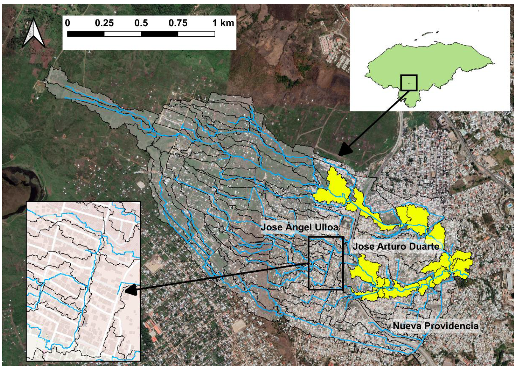
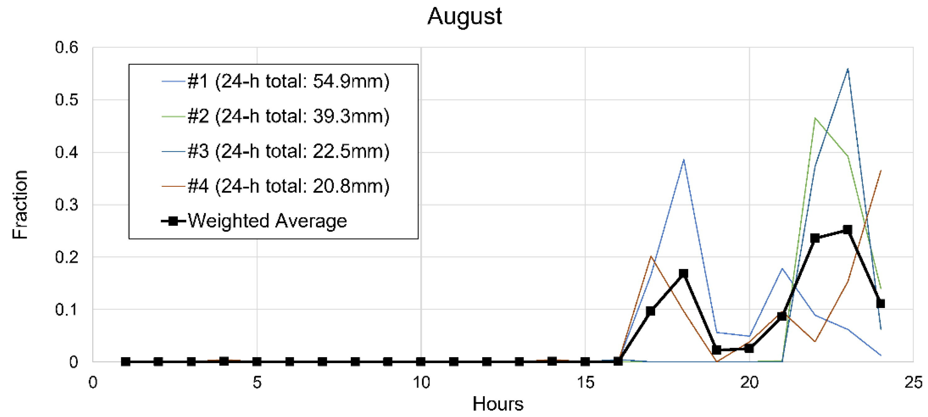
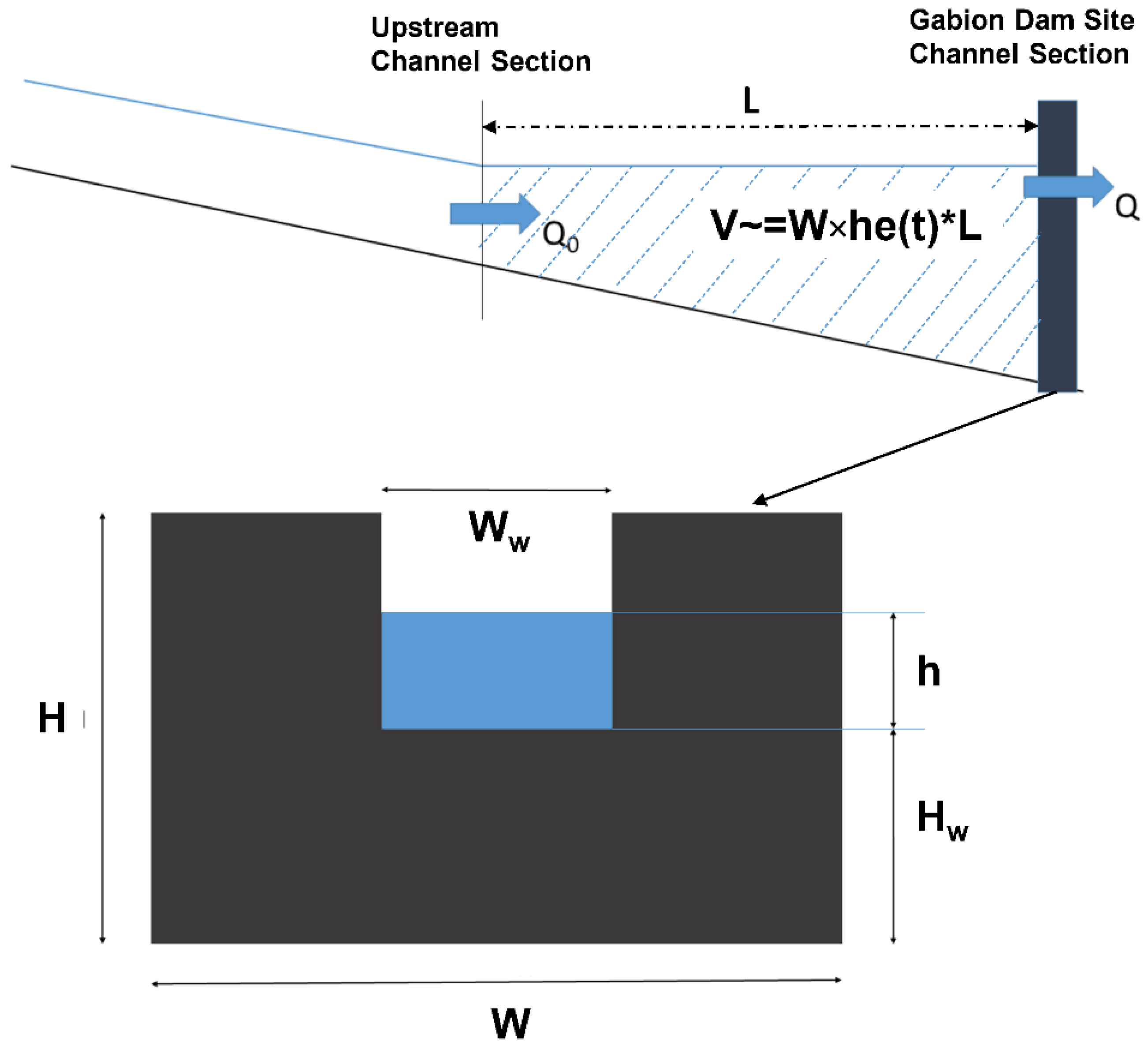
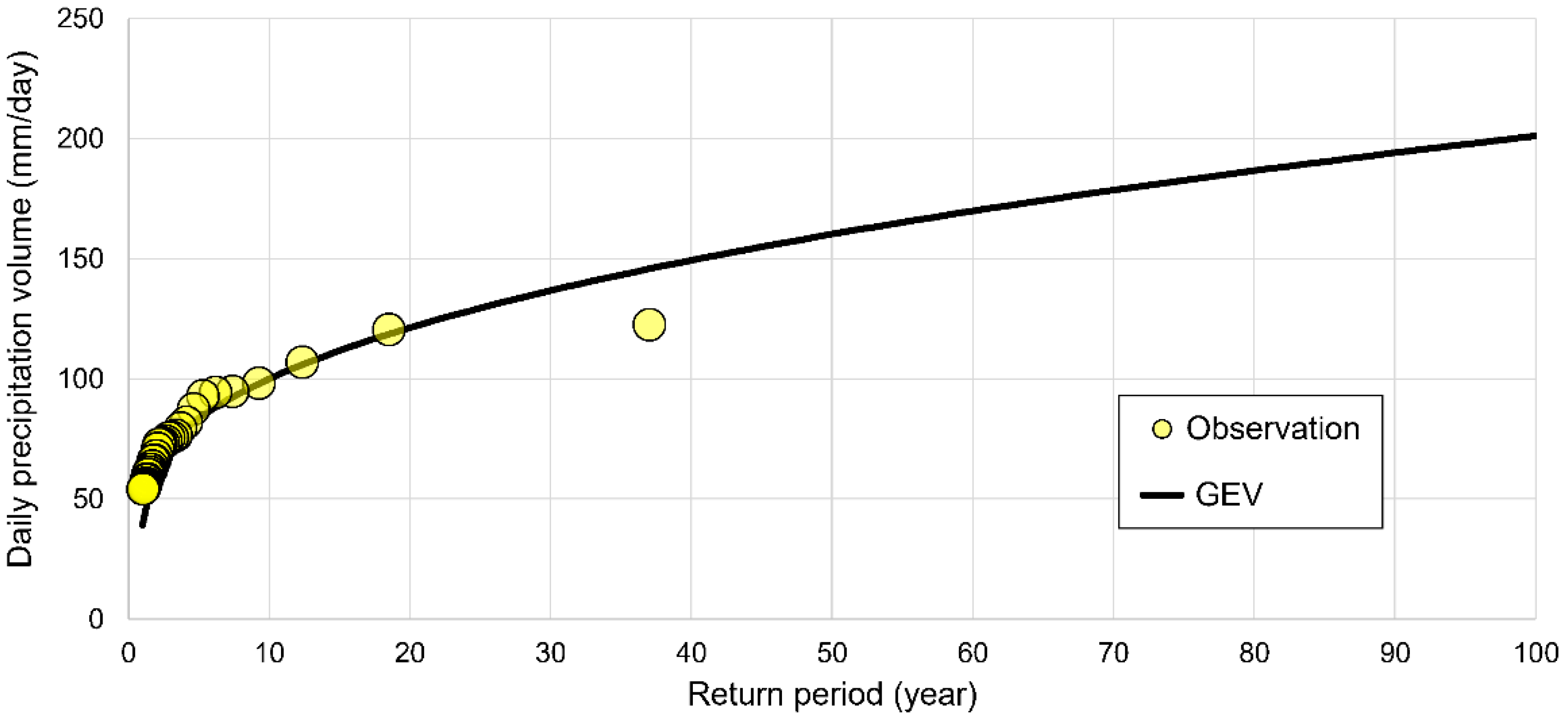
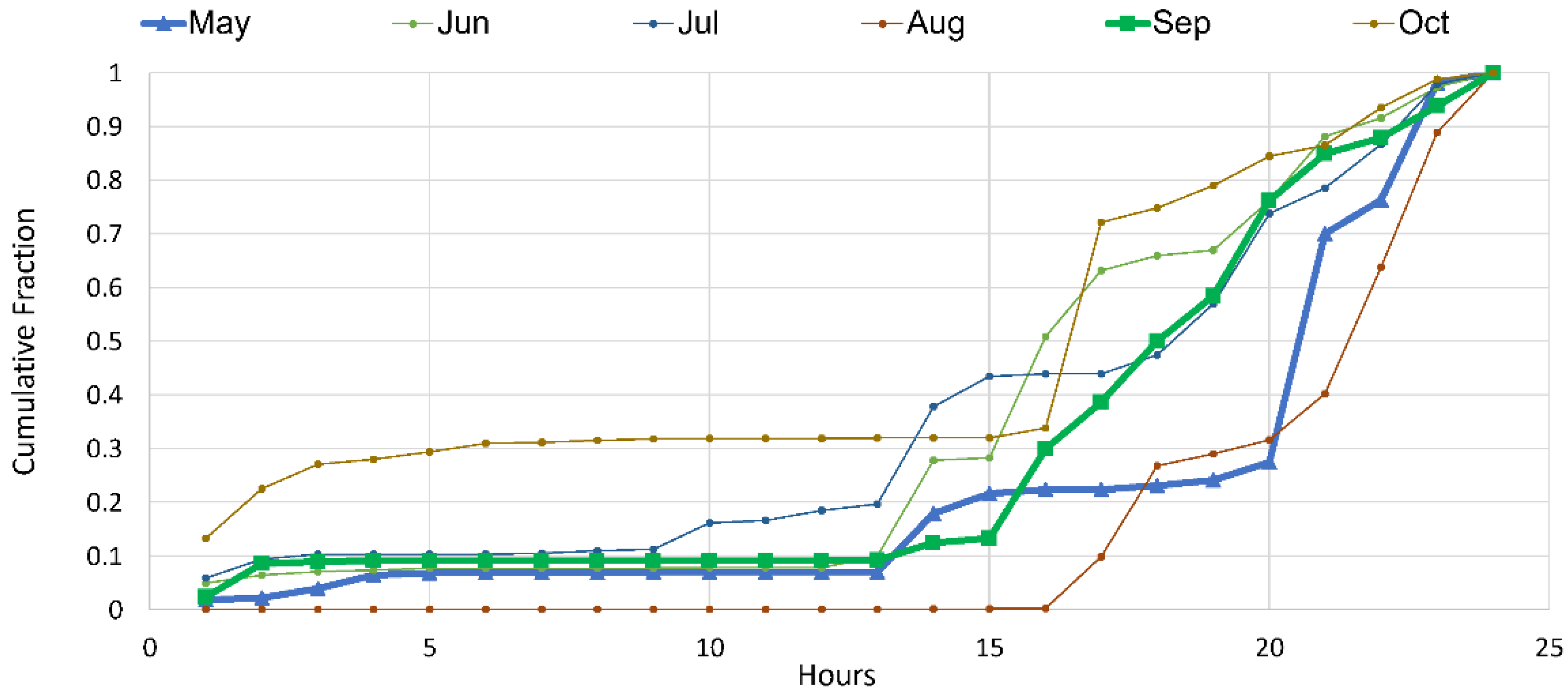
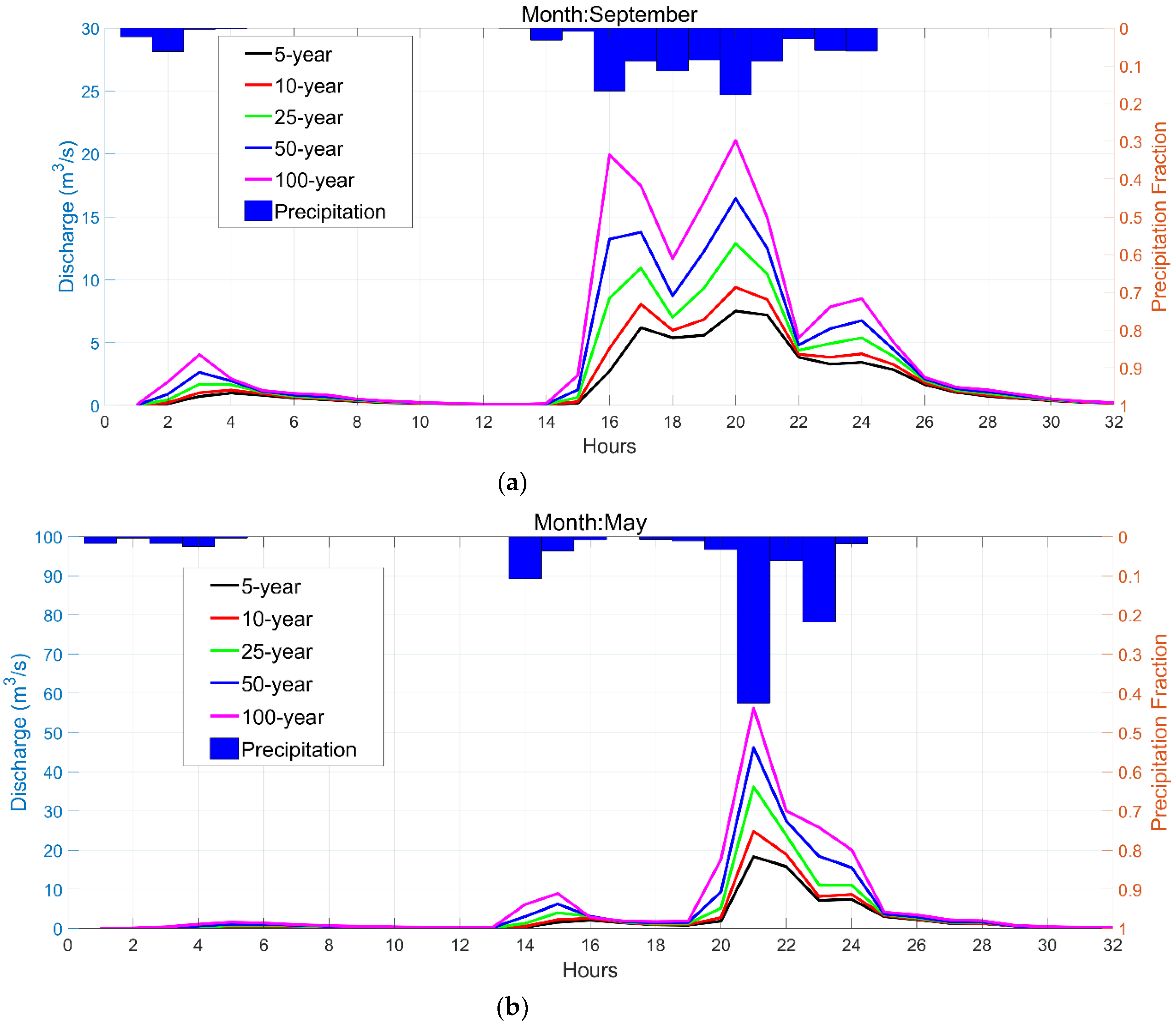
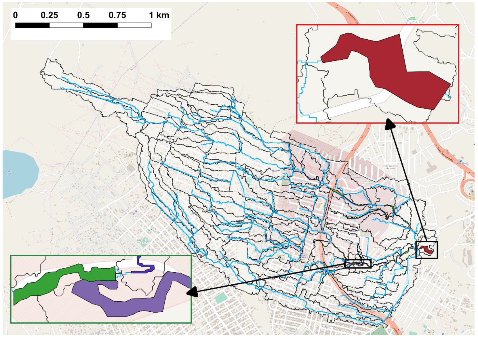
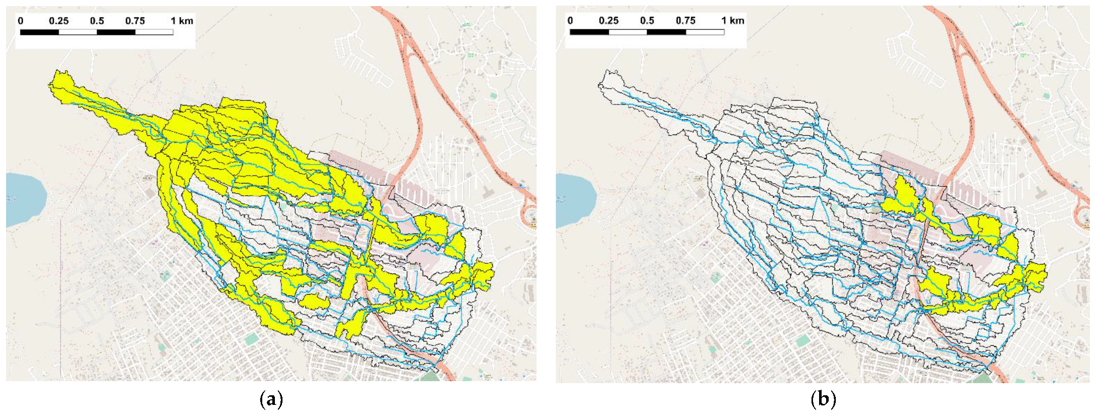
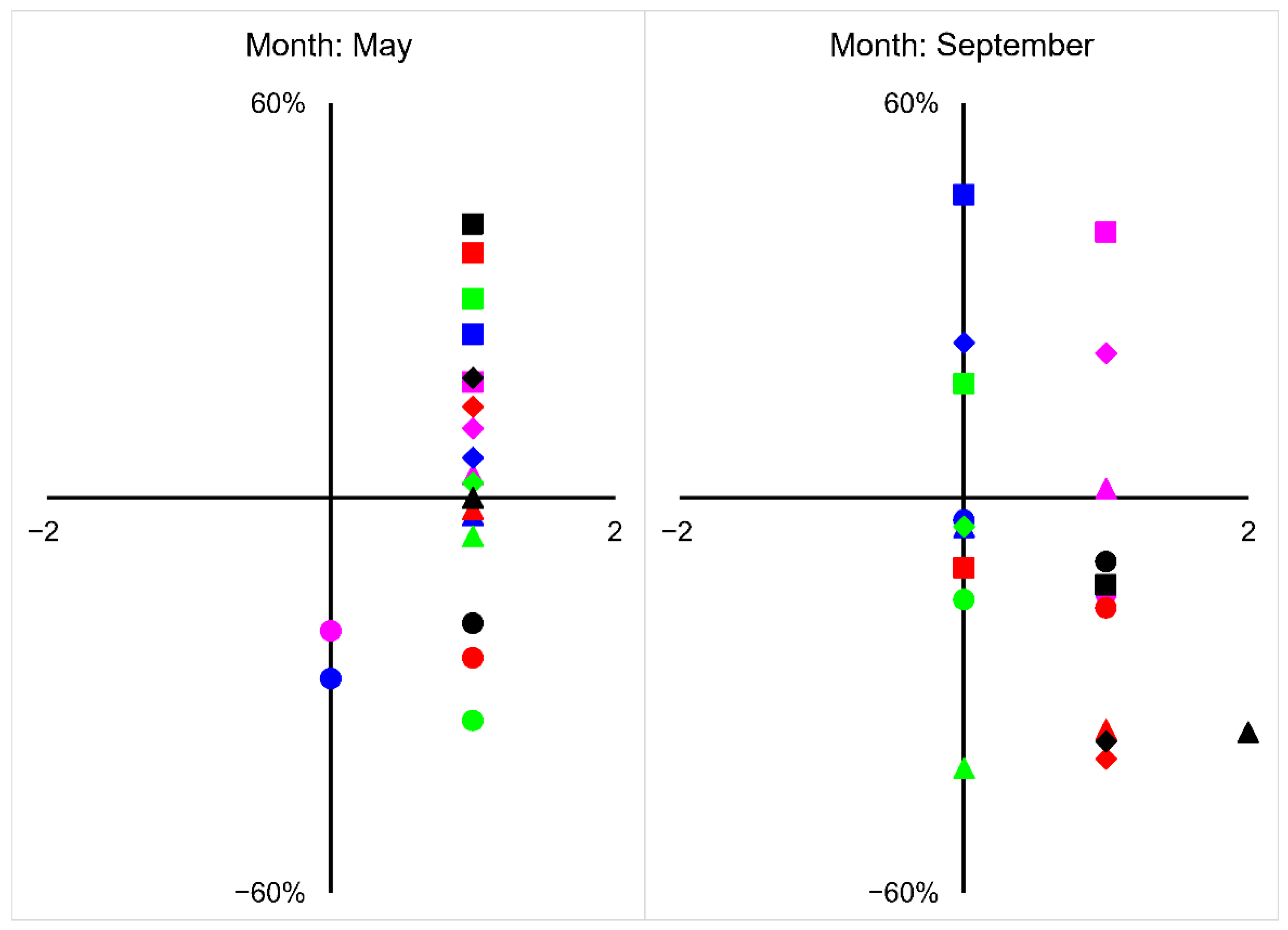
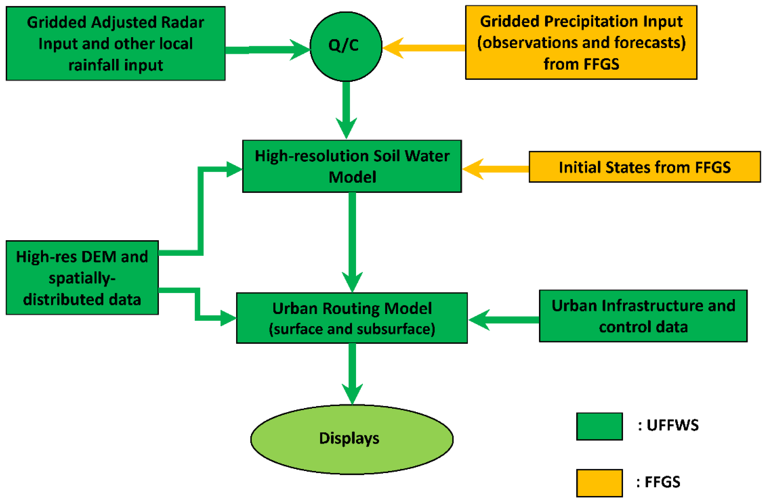
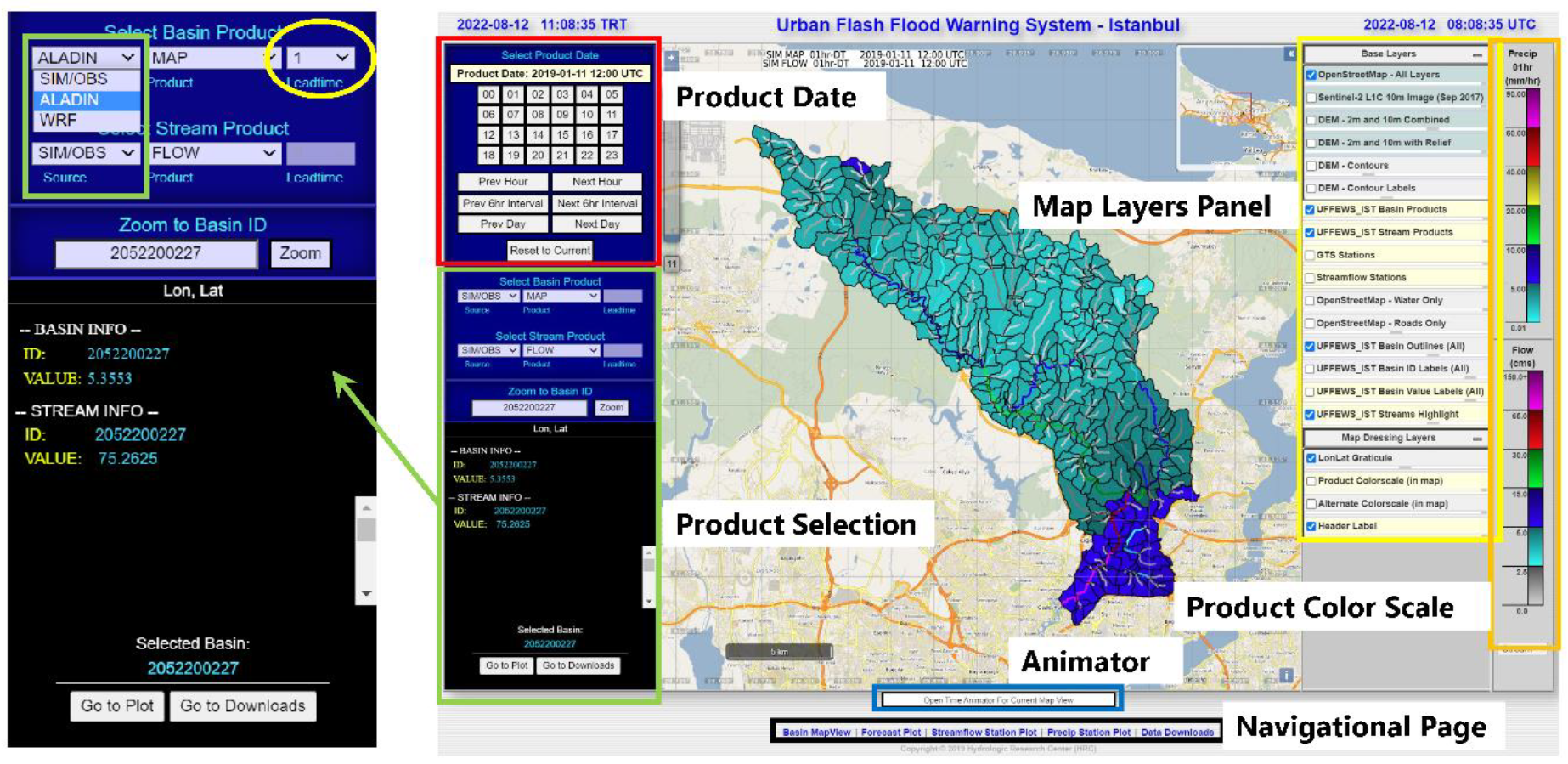
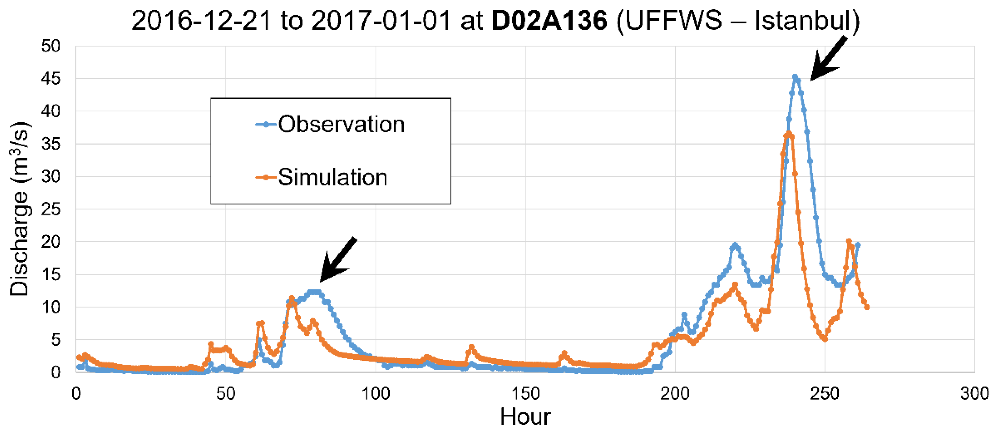
Table 1.
Parameters of the Sacramento (SAC) soil water accounting model for the region.
| UZTWM (mm) | UZFWM (mm) | LZTWM (mm) | LZFPM (mm) | LZFSM (mm) | UZK (Fraction) | LZPK (Fraction) | LZSK (Fraction) | ZPERC | REXP | PFREE (Fraction) | SIDE (Fraction) | ADIMP (Fraction) |
|---|---|---|---|---|---|---|---|---|---|---|---|---|
| 9 | 5.4 | 36 | 15.22 | 6.38 | 0.145 | 0.000651 | 0.0453 | 85 | 2.5 | 0.295 | 0 | 0.05 |
Table 2.
Dimensions (m) of gabion dams and associated detention basin reservoirs (see Figure 6).
Table 2.
Dimensions (m) of gabion dams and associated detention basin reservoirs (see Figure 6).
| Length of Reservoir (L) | Width of Reservoir (W) | Width of Weir (Ww) | Height of Weir (Hw) | Total Height (H) |
|---|---|---|---|---|
| 50 | 10 | 1 | 2 | 3 |
Table 3.
Coefficients of linear regression between elevation and mean monthly daily precipitation average for each month.
Table 3.
Coefficients of linear regression between elevation and mean monthly daily precipitation average for each month.
| Month | α (1/d) | β (mm/d) |
|---|---|---|
| JAN | 0.002029 | −2.041 |
| FEB | 0.001084 | −1.122 |
| MAR | 0.001389 | −0.9467 |
| APR | 0.0008147 | −0.9621 |
| MAY | 0.003453 | 1.013 |
| JUN | 0.007451 | −3.268 |
| JUL | 0.003383 | −2.179 |
| AUG | 0.002351 | 2.348 |
| SEP | 0.005956 | −0.5184 |
| OCT | 0.007418 | −2.796 |
| NOV | 0.002696 | −1.995 |
| DEC | 0.001937 | −1.505 |
Table 4.
Reference values of the total volume (mm) of the 24-h design storms.
| 5-Year | 10-Year | 25-Year | 50-Year | 100-Year |
|---|---|---|---|---|
| 83.64 | 99.98 | 129.46 | 160.21 | 201.08 |
Table 5.
Largest inundation width (m) near the outlet of the outlet of the area estimated using peak discharge in May.
Table 5.
Largest inundation width (m) near the outlet of the outlet of the area estimated using peak discharge in May.
| Nominal | Revegetation (All) | Gabion (All) | Revegetation + Gabion (All) | Revegetation + Gabion (Selected) |
|---|---|---|---|---|
| 27.27 | 26.25 | 27.75 | 27.43 | 28.18 |
Table 6.
Values of reference peak discharge (m3/s) under different design storms.
| 5-Year | 10-Year | 25-Year | 50-Year | 100-Year | |
|---|---|---|---|---|---|
| May | 18.3 | 24.8 | 36.2 | 46.2 | 56.3 |
| September | 6.19 | 8.05 | 10.9 | 13.2 | 19.9 |
Publisher’s Note: MDPI stays neutral with regard to jurisdictional claims in published maps and institutional affiliations. |
© 2022 by the authors. Licensee MDPI, Basel, Switzerland. This article is an open access article distributed under the terms and conditions of the Creative Commons Attribution (CC BY) license (https://creativecommons.org/licenses/by/4.0/).
Share and Cite
MDPI and ACS Style
Cheng, Z.; Georgakakos, K.P.; Spencer, C.R.; Banks, R. Numerical Modeling of Flash Flood Risk Mitigation and Operational Warning in Urban Areas. Water 2022, 14, 2494. https://doi.org/10.3390/w14162494
AMA Style
Cheng Z, Georgakakos KP, Spencer CR, Banks R. Numerical Modeling of Flash Flood Risk Mitigation and Operational Warning in Urban Areas. Water. 2022; 14(16):2494. https://doi.org/10.3390/w14162494
Chicago/Turabian StyleCheng, Zhengyang, Konstantine P. Georgakakos, Cristopher R. Spencer, and Randall Banks. 2022. "Numerical Modeling of Flash Flood Risk Mitigation and Operational Warning in Urban Areas" Water 14, no. 16: 2494. https://doi.org/10.3390/w14162494
Note that from the first issue of 2016, this journal uses article numbers instead of page numbers. See further details here.