
Impact of Fish Ponds on Stream Hydrology and Temperature Regime in the Context of Freshwater Pearl Mussel Conservation


1
Aquatic Systems Biology, TUM School of Life Sciences, Technical University of Munich, Mühlenweg 22, 85354 Freising, Germany
2
Hydrology and River Basin Management, Faculty of Civil, Geo and Environmental Engineering, Technical University of Munich, Arcisstraße 21, 80333 Munich, Germany
*
Author to whom correspondence should be addressed.
Water 2022, 14(16), 2490; https://doi.org/10.3390/w14162490
Submission received: 8 July 2022
/
Revised: 6 August 2022
/
Accepted: 10 August 2022
/
Published: 12 August 2022
(This article belongs to the Section Water, Agriculture and Aquaculture)
Abstract
:Conservation of endangered, cold-stenothermic species, such as the freshwater pearl mussel (FPM) and its salmonid host fish, are particularly challenging in headwater streams as their last refuge areas. Understanding the impact of anthropogenic catchment features such as fish ponds on the hydrology and the temperature regime of such streams is, therefore, important. In this study, runoff in a FPM catchment with more than 150 small ponds was simulated using SWAT and compared to a scenario without ponds. Additionally, water temperature was monitored hourly along three steams over 2.5 years, at sites upstream and downstream of the inflow of pond outlet channels. Temperature metrics were related to land use within a 180 m corridor along the streams. Peak flows were reduced by 1.5% with ponds, while low flows were increased by 4.5%. In summer, temperature in pond effluents was higher than in the receiving stream, depending on the proximity of the inflow points. Discharge from close-by ponds increased summer stream temperature directly downstream of the inflow by up to 5.5 °C. These increased temperatures were partly compensated by groundwater contribution in forested areas. In contrast, stream temperature significantly further increased along stretches flowing through open land, persisting independently of pond inflows. We suggest incorporating this knowledge on pond- and land use-dependent effects on stream temperature regimes into the conservation management of FPM and other cold-stenothermic species, as well as into climate change mitigation strategies targeting an increased resilience against temperature extremes.
1. Introduction
Increasing global air temperature due to anthropogenic climate change has affected freshwater ecosystems worldwide [1], making the management of flow and temperature regimes—and particularly of cold-water spots in streams and rivers during summer—a key priority for the sustainable management of cold-stenothermic species [2,3,4,5,6]. An intensification of the hydrological cycle can have pronounced effects on waterbodies, causing chances in regional patterns of evapotranspiration and precipitation, increasing the probability of extreme events such as floods and droughts [7]. In particular, low flows can have adverse effects on stream biodiversity [8], by reducing water and habitat quantity [9] which might be mitigated by increased water retention at the landscape scale [10,11,12]. Small waterbodies such as ponds and wetlands influence evaporation, groundwater recharge and flood retention [13,14], offering an option for drought mitigation [15,16]. On the other hand, they may contribute to the warming of receiving streams, potentially counteracting their effects of buffering low flows. To help incorporating the multiple, interacting effects of ponds and other catchment features such as land use (LU), hydrological modeling at the catchment scale can help evaluating effects and assist with the planning of pond construction. Modelling tools such as the Soil and Water Assessment Tool (SWAT) can be used to model whole catchments and then compare water or sediment yield between certain LU or climate scenarios [17,18,19,20]. Nonetheless, since hydrological modeling needs to generalize many parameters at a broad scale to ensure efficient computing, it can be challenging to analyze the impact of individual ponds through this catchment-scale approach. Field measurements on specific ponds of interest might be needed to ensure an accurate representation of pond effects at the local scale. Water temperature (Tw) measurements are ideally suited for this purpose, simultaneously providing additional information on ecological impacts of pond effluents, as hydrology and temperature regimes are coupled. Temperature surveys using automatic temperature loggers have become an easy and cost-efficient measure to obtain data at a high spatial and temporal resolution [21]. Numerous studies used this approach to investigate groundwater contribution to streamflow (e.g., [22]), the impact of heated effluent discharge [23], or the impact of impoundments and ponds [24] at the reach scale. Moreover, the thermal regime of streams is, by itself, an important parameter shaping aquatic communities. Climate change might impact the hydrologic regime, with increasing periods of low flow conditions resulting in reduction or complete loss of habitat for cold-stenothermic species such as salmonids [4]. Furthermore, rising air temperatures directly cause increased warming of surface water bodies [25] and changes in stream thermal regimes [26]. Increasing Tw has direct impacts on stream organisms by lowering oxygen solubility [27] and thus the physicochemical habitat quality as well as by enhancing the metabolic rate of poikilothermic species. It can also shift competitive advantages of invasive versus native species (e.g., [28]). Tw therefore plays a key role in structuring aquatic communities and in determining species distribution [9,29,30,31,32]. However, it is difficult to interpret in an ecological context as single or mean values might be insufficient to determine ecological impacts. The thermal regime accounts for diel, daily, seasonal and annual variation as well as spatial patterns along the stream course [33,34]. It might not only be relevant if a certain temperature threshold is exceeded, but also if the threshold is exceeded during a critical time in a target species life cycle [35]. Predicted increases in global Tw vary between 1.0 and 4.0 °C by 2050, depending on climate change scenario [36,37,38]. Prolonged low flow periods additionally enhance stream warming by decreasing thermal capacity [1]. This is mainly a threat to cool-stenothermal organisms adapted to cool thermal regimes such as the highly endangered freshwater pearl mussel Margaritifera margaritifera (FPM). This species and its fish host require summer Tw < 20 °C in most of their Central European and Scandinavian range [39]. Higher Tw are associated with low numbers of gravid females in non-recruiting populations [40]. Moreover, successful reproduction of this species strongly depends on the presence of its salmonid host fish, the brown trout Salmo trutta or the Atlantic salmon Salmo salar, in close proximity to mussel beds during the spawning period, since the FPM life cycle includes a parasitic phase of its glochidia larvae on the host fish’s gills [41]. Salmonids such as the brown trout are adapted to cold water temperatures with a temperature optimum between 12–18 °C [42] and with the upper critical temperature limit between 22–25 °C [43]. They were shown to avoid reaches with summer Tw over 21 °C and search for thermal refugia with cooler Tw [44,45]. In Central Europe, the FPM usually release their glochidia between June and September, when Tw are at their maximum [46]. If the highly sensitive brown trout avoids reaches populated by FPM due to Tw above its thermal tolerance, infestation with glochidia cannot take place and natural reproduction ceases. Moreover, the survival and attachment ability of mussel glochidia also strongly depends on ambient Tw [47] and it has been shown that Tw is crucial for the performance and timing of excystment of metamorphosed juvenile mussels from their fish hosts [48,49]. Insufficient levels of natural reproduction are the major cause of the strong declines in the last remaining FPM populations within the species Central European distribution [41]. However, Tw that are too cold also impair or delay reproduction, with a sufficient number of days with Tw > 10–15 °C needed for maturation [46] and sufficient growth of juveniles [50,51].
The European drought during the summers of 2018 and 2019 [52] showed the urgent need to find ways to increase the resilience of headwater streams to drought. In particular, in north-eastern Germany as well as in north-east Bavaria low soil moisture levels and stream water levels threatened the last remaining FPM populations in the area, which represent some of the largest remaining in Central Europe. To prevent reaches inhabited by the FPM from falling dry, water was discharged from nearby ponds and deep wells that are usually used for drinking water abstraction. This development is critical because the small headwater streams concerned are the last refuges of cold-water species in this area as they are dominated by groundwater inflow during summer [53]. The presence of more than 150 ponds in the catchment of the FPM streams raised the question to what extent they have an impact of the runoff and Tw of these valuable ecosystems. While most of the attention concerning the effect of heated effluents is focused on the impact of power plants [54,55] and damming [56,57,58], the impact of pond effluents on water temperature of adjacent streams has received little attention, despite the high number of ponds all over the globe [59]. Various impacts of ponds on hydrological and temperature regime are suggested, depending on multiple parameters as well as on other LU features, but there is still limited understanding of LU-pond-stream interactions [60].
In this study, the impacts of multiple ponds within a small catchment with FPM were assessed through a catchment-wide hydrological modelling using SWAT as well as a field survey of Tw at multiple sites and compared with other LU features within the catchment. To our knowledge, this is the first study combining an evaluation of the impact of ponds on the hydrological and temperature regime at the catchment as well as the local scale with a focus on the critically endangered FPM. The following hypothesis were tested:
- Ponds have a significant influence on the hydrological cycle at the catchment scale, increasing flood retention during high flows and buffering low water levels during low flow conditions.
- Ponds have an impact on the temperature regime in small, cool, headwater streams, with significant increase in stream temperature through ponds effluents in summer and nearly neutral effects during winter.
- Effects on hydrological and temperature regime accumulate with increasing number of ponds draining into a stream.
2. Materials and Methods
2.1. Study Area
The catchment of the “Schwesnitz” river, a tributary of the Sächsische Saale of the Elbe stream was chosen for this study as it contains more than 150 individual ponds, as well as populations of the endangered FPM, making it a priority area of conservation. It is formed by the two major tributaries “Perlenbach” coming from the south and “Höllbach” coming from the Czech Republic in the east (Figure 1). The mean annual precipitation sum and temperature at the meteorological station “Hof” (ID 2261) are 757.6 mm and 7.1 °C, respectively. The long-term mean annual discharge at the gauging station “Schwesnitz” (50.245433° N 12.019682° E) is 0.67 m3/s. The discharge regime is dominated by higher flows in winter and in particular after the snow melt, and lower flows during summer and autumn, when groundwater dominates the baseflow [53]. The total catchment area of 90.82 km2 is dominated by coniferous forest, primarily spruce (50.4%), followed by agricultural LU (22.6%) and pastures (18.8%) according to the satellite-derived CORINE 2012 Land Cover map [61]. 150 earthen ponds are located within the study catchment, with an average size of 1384.6 m2 (range: 39.5–46,101.4 m2). They are mostly used for extensive carp production, meaning they remain filled year-round except for a period of about one week, when water is drained for fish harvest [62]. Some of the ponds are managed as flow-through ponds, with a constant small amount of water discharged to the receiving streams, while in some ponds, water is only supplied to compensate for evaporation losses and the outflow is closed during low discharge conditions in summer.
2.2. Hydrological Model Setup
To model the hydrological regimes of the catchment, the Soil and Water Assessment Tool (SWAT, [63]) was used through geoinformatic software ArcMap 10.5.0 (Esri, Redlands, CA, USA) using the software extension ArcSWAT [64]. The SWAT model is a physically based model, relying on a digital elevation model (DEM) to delineate the stream network and the associated catchment, which is then divided into smaller subbasins. The model further incorporates LU and soil maps, as well as slope and climate data. Each subbasin is further divided into so-called hydrological response units (HRUs), each consisting of a unique combination of LU, soil and slope categories that are used to model hydrological processes for each HRU. The surface runoff generated in each HRU is then routed through the stream network of the different subbasins until it reaches the catchment outlet. The model was set up using the following input data:
The DEM used in this study was merged from two sources, a 1 × 1 m DEM covering the German part of the catchment provided by the water authorities board (WWA) in Hof and an 5 × 5 m DEM covering the Czech part of the catchment provided by the Czech Office for Surveying, Mapping and Cadaster. Both raster data sets were merged into one data set with a 5 × 5 m resolution. The complete DEM was used to delineate the stream network and subbasins based on a 50-ha threshold to achieve the maximum possible channel resolution. Four slope categories were derived based on the DEM.
LU was obtained from the CORINE Land Cover CLC 2012 data set ([61], Figure 1) and converted into the SWAT LU classification.
The soil map was obtained by merging the soil map BÜK25 provided by the Bavarian Environmental Agency for the German part and the soil map CR50 provided by the Czech geological survey. Hydrological soil groups for the German part were provided by the WWA Hof. German and Czech soil classes were harmonized based on particle size.
Based on these data sets, an initial SWAT model was set up for the 90.82 km2 Schwesnitz catchment, comprised of 87 subbasins and 1889 HRUs, based on a threshold of 3% for each LU, soil and slope category. Daily precipitation data for the period between 2008–2021 was obtained from four meteorological stations of the German National Meteorological Service within or close to the study catchment (Station “Hof”, ID: 2231; Station “Selb”, ID: 4548; Station “Rehau”, ID: 4109; Station “Regnitzlosau”, ID: 4107; Figure 1). Data on daily minimum and maximum air temperature and relative humidity was only available for the stations at “Hof” and “Selb” and daily wind speed data was only available for the “Hof” station. Solar radiation data was simulated within the SWAT weather generator, since no small-scale observation data was available for this parameter. Therefore, the Hargraves method was chosen for calculating potential evapotranspiration (PET), which is only based on daily minimum and maximum temperature [63]. The initial model was run with a warm-up period of two years.
SWAT allows the integration of one pond or wetland per subbasin [63,65]. Spatial data on the location and surface area of the ponds found within the catchment was obtained from orthophotos and field observations. When multiple ponds occurred within one subbasin, they were combined to form a hydrological equivalent wetland (HEW, [66]). In total, 68 of the subbasins contained at least one pond. The pond parameter PND_FR, quantifying the proportion of the subbasin area draining into the pond, was obtained from the DEM using the Flow Path Tracing tool of ArcHydro. The other parameters describing the ponds were derived from the pond map, field observations or literature and are listed in Table 1.
2.3. Calibration and Validation
The calibration and uncertainty analysis software SWAT CUP (V 5.2.1.1, 2w2e GmbH 2019) was used to calibrate the initial models’ parameters to accurately simulate the runoff values at subbasin 32 compared to those observed at the gauging station “Schwesnitz” (provided by the Bavarian Waterscience Service, available at www.gkd.bayern.de (accessed on 12 April 2022)). A sensitivity analysis was performed prior to the calibration to identify the relevant parameters. These were included into the calibration process, together with several parameters chosen after a literature review. For the pond parameters, only PND_K showed a significant effect and was included into the calibration. The parameters used in the calibration process can be found in Table 2.
Five iterations with 300 simulations each were performed using the SUFI-2 algorithm on daily runoff data for the period from 1 January 2015 to 31 December 2021. The results were validated for the period from 1 January 2010 to 31 December 2014.
To evaluate the effect of the ponds on the hydrologic regime, daily runoff at subbasin 32 was compared between the existing scenario with ponds (used for calibration) and a scenario without ponds, where the calibrated parameters were used in the simulation but PND_FR was set zero in all subbasins, which turns off the pond function [65]. To differentiate between effects at high, peak, and low flows, runoff conditions were classified using long-term statistical thresholds (see also [68]), as well as the maximum flow for each high discharge event.
2.4. Temperature Measurements
To obtain Tw for assessment of the temperature regime upstream and downstream of the inflow of pond outlet channels, a total of 31 temperature loggers (EL-USB-1, Lascar Electronics, Salisbury, UK) with accuracy of Tw ± 0.5 °C and logging interval of 60 min were employed between spring 2018 and autumn 2020. At twelve monitoring sites (Figure 1), loggers were installed upstream (‘us’) and downstream (‘ds’) of the inflow of several pond outlet channels, following the study design described by [62]. Where possible, an additional logger was installed directly within the pond outlet channel. Five sampling sites were established in the BB, one tributary of the “Perlenbach”. The upper part of the stream is dominated by a big fish farm consisting of more than 25 ponds. Along its course through a mostly forested area, multiple pond facilities drain into the stream. Towards the confluence with the “Perlenbach”, the catchment LU around the BB changes to open, agriculturally used lands. In contrast, the MB, a tributary of the “Höllbach”, originates from an open wetland area, then flows through coniferous forest. Multiple ponds drain into the MB along its course, where three sampling sites were established until the confluence with the “Höllbach”. Along the course of the “Höllbach” (HB), four sampling sites were established, including one at a tributary (EB) and one the confluence with the MB. At EB1, the main stream received inflow from two pond facilities from two different side channels. Furthermore, the monitoring site EB1 is close to a deep well, from which groundwater was discharged during summer 2018 and 2019 to support streamflow. Moreover, due to the drought conditions water discharge from several ponds was decreased to sustain conditions needed for fish farming, causing the complete cessation of discharge from the pond MB1.
2.5. Data Analysis
The hourly measured Tw values were compared between the monitoring points at each site. Furthermore, delta Tw (ΔTw) was calculated between subsequent temperature loggers (X − 1 > X > X + 1) by subtracting the value measured by the logger at the position upstream (T − 1) from the value measured at position T at a given date and time once within sites (site X ds—site X us) as well as between sites (site X us—site X − 1 ds; Figure 1).
The hourly measurements of Tw were also summarized as daily mean, minimum and maximum data and then used to calculate 12 metrics describing the general temperature regime and aspects of interest within the context of FPM at the respective monitoring points using an adapted version of the StreamThermal package in R (Table 3). Delta values of these metrics between subsequent monitoring points were calculated as described above. Pearson’s correlation test was used to analyze the relationship between temperature metrics and pond or LU characteristics, assuming a linear relationship. Multivariate analysis of the summer thermal regime was conducted using an agglomerative hierarchical clustering analysis of monitoring points based on the standardized/normalized summer metrics. The cluster analysis was performed in PRIMER 7 Version 7.0.17 (Plymouth Marine Laboratory, Plymouth, UK) on Euclidean distance using the Group Average joining algorithm following [69].
To assess the potential influence of LU on Tw, the proportion of LU types were calculated within a 180 m corridor around the streams using ArcMap 10.5.0. (Esri, Redland, CA, USA, Figure 1) using pond spatial data and CORINE data (summarized into two categories: forested area: coniferous and mixed-forest, open land: pasture and arable land). Distance between the pond outlets and the ‘out’ monitoring sites was calculated and grouped into three categories: “close”: pond < 50 m from the monitoring site; “medium far”: pond 400–600 m from the monitoring site and “far”: pond > 1000 m from the monitoring site.
A multiple linear regression model including the proportion of pond and forested area (the proportion of open land was excluded due to high collinearity with the proportion of forested area), the reach length and the interaction between all three variables was run to evaluate the impact of the variables on the difference in average daily mean temperature in summer (Δ ADM_su) between two subsequent monitoring points. Model performance was evaluated by standard graphical validation [70] and the ‘DHARMa’ diagnostic package. A significance level of alpha = 0.05 was set for all statistical analysis.
For analyzing patterns of Tw changes along the stream course, a complete set of ΔTw for all monitoring points within one stream was prepared. Periods for the three streams were chosen to maximize the time span of all loggers within one stream to deliver continuous data. This resulted in the study period for BB being from the 11 June 2019–1 September 2020, for MB being from 18 June 2018–21 May 2019 and for HB being from 24 November 2018–20 August 2019.
Radon was used as a tracer for groundwater discharge in the study catchment between 2019 and 2020 [53]. Since groundwater discharge has a considerable influence on Tw [71,72,73], in particular during low flows, the output of the SWAT model was used to calculate the baseflow index (BFI) in 2018, 2019 and 2020 for subbasins representing the stretches between monitoring sites, where applicable. BFI was calculated using the lfstat package in R, as recommended by the WMO [74]. Since the BFI for the subbasins representing the stretches along the MB that matched the stretches in the radon study [53] showed a similar pattern as the radon-based groundwater discharge, the BFI was used as a proxy for groundwater discharge in all other subbasins of the present study (Supplementary Materials Table S1). Differences in BFI between stream sections were assessed in R Version 4.1.0 (www.r-project.org (accessed on 18 May 2021), 2021) using Kruskal-Wallis with post-hoc Mann-Whitney U-test with Bonferroni correction, as the data were not normally distributed and variances inhomogeneous.
3. Results
3.1. Hydrologic Regime
The model evaluation parameters for the calibrated model are given in Table 4. The calibrated model with ponds was classified as “good” or “very good” for five of six widely used evaluation criteria [75] for daily stream flow, with NSE of 0.71 and 0.77 for the calibration and validation period, respectively. For the validation period, only PBAIS of 16.2 was “not satisfactory” due to an overestimation of low flows (Figure 2). Since the field campaign took place during the calibration period, when all three parameters classified the model as “good” or “very good”, the stream flow modeled for the subbasins of interest were considered valid for further analysis.
Within the 68 subbasins containing a pond, the average proportion of subbasin area draining into a pond (PND_FR) was 41.4%, representing 26.3% of the total catchment area. Mean HEW size was 0.094 ha and varied between 0.059–0.151 ha. When the ponds were included, the model simulated stream flow that was on average 3.2% higher than in the scenario without ponds. Separating between high and low flow conditions (based on the long-term statistics of the gauging station) revealed a more differentiated pattern: Over all higher flows, the stream flow with ponds was 0.2% lower than without ponds while the peak flows were decreased by 1.5% with ponds. In contrast, stream flow under low flow conditions was on average 4.5% higher with ponds than without them. The ponds therefore moderately increased low flows while the buffering effect during the peak flows was relatively low. Concerning the timing of floods, no differences could be observed between the two models. In the scenario without ponds, 16 days were additionally classified as days with high flow conditions over the whole simulation period, which represented a shift from 20.3 to 21.0% compared to the scenario with ponds.
The BFI values were calculated using the hydrographs simulated by the model with ponds in 2018, 2019 and 2020 for 13 subbasins matching the temperature monitoring campaign. (Supplementary Materials Table S1). Average BFI over all reaches was 0.79 ± 0.07 over the whole modeled period. Considering BFI in the temperature-study stretches in 2018–2020 revealed a strong temporal differentiation: While groundwater contribution in 2018/19 was on average 91 ± 9% during the extreme low flow conditions, it decreased to 54 ± 8% in 2020. Highest BFIs were observed in the upstream regions of the MB and BB, with slightly lower values towards the downstream reaches and in the HB. However, the values did not differ significantly between upstream and downstream reaches of the respective streams in neither of the years (Mann-Whitney U-test, p-values > 0.05).
3.2. Temperature Regime
In 2018, after a dry and warm spring, water levels dropped below the mean low water levels from the end of July until mid-November. Mean daily air temperatures at the climate station “Hof” reached values > 20 °C during in July and August, with a maximum of 26.6 °C and only minimal precipitation occurring in summer and autumn [76]. In the subsequent winter, low temperatures (mean daily air temperatures down to below −7.0 °C) and increased discharge were accompanied by snowfall, but this period of rather high discharges was followed by another dry spring and extremely hot summer in 2019. Water levels in the study streams decreased to even lower values, with stream segments drying out completely in a neighboring stream system (see [68]) and stream flow in the study streams only sustained due to intervention by the water authorities discharging water from adjacent ponds and pumping from deep wells. Increased precipitation alleviated the situation from September onwards, moving towards a period of higher precipitation rates and well sustained stream flow levels during autumn, winter and the subsequent spring and summer 2020, when mean daily air temperatures > 20 °C were only reached during August.
The average summer temperature regime differed between the monitoring points at the inflow of ponds effluents. ADM_su among monitoring points within the pond outlet channels was 16.8 ± 2.4 °C and therefore higher than in the main stream, where mean ADM_su at ‘us’ monitoring points was 15.2 ± 1.5 °C and 15.5 ± 1.0 °C at ‘ds’ monitoring points. The mean difference between ‘us’ and ‘ds’ was 0.5 ± 1.3 °C, indicating increased Tw downstream of the pond outlet channel inflow. Average MaxD_su at ‘out’ was 20.7 ± 2.5 °C, with AMax_su reaching 18.4 ± 2.1 °C. The highest ever measured Tw within the study period was 27.5 °C at the site BB5_out. Average MaxD_su and AMax_su at ‘us’ sites were 18.6 ± 1.8 °C and 17.0 ± 1.7 °C and 19.1 ± 1.2 °C and 17.3 ± 1.1 °C at ‘ds’, respectively. The mean range_su was 3.0 ± 0.7 °C for ‘out’, 3.5 ± 0.6 °C for ‘us’ and 3.4 ± 0.6 °C for ‘ds’ monitoring points. MaxT was reached on average on day 209 ± 24 for ‘out’, on day 209 ± 20 for ‘us’ and on day 207 ± 25 for ‘ds’ monitoring points. On average, Tw was below 14.5 °C for 21 ± 21 of the days of summer at ‘out’, for 33 ± 22 days at ‘us’ and for 26 ± 16 days at ‘ds’ monitoring points. Tw of 20 °C or higher was reached at 24 ± 21 of the days of summer at ‘out’, at 9 ± 12 days at ‘us’ and at 8 ± 8 days at ‘ds’ monitoring points.
In winter, ADM_wi was 2.8 ± 1.0 °C at ‘out’, 2.9 ± 0.6 °C at ‘us’ and 2.8 ± 0.6 °C at ‘ds’ monitoring points. MaxD_wi at ‘out’ was 5.6 ± 0.7 °C, with AMax_wi reaching 3.3 ± 1.0 °C. Average MaxD_wi and AMax_wi at ‘us’ sites were 5.8 ± 0.4 and 3.5 ± 0.6 and 5.7 ± 0.4 and 3.4 ± 0.6 °C at ‘ds’, respectively.
However, all metrics showed a high site variability (Table 5, Figure 3) with the impact of the pond discharge on the receiving stream ranging from an increase of ADM_su downstream of up to 2.6 °C to a decrease of 2.9 °C. Therefore, an analysis of the monitoring sites was conducted via cluster analysis to identify underlying patterns.
Of the 11 monitoring points within the pond outlet channels, six were categorized as “close” to the pond with a mean distance between pond outlet and the ‘out’ monitoring site of 25.5 ± 12.8 m, three were categorized as “medium far” with a mean distance of 536.0 ± 62.0 m and the remaining two as “far” with a mean distance of 1757.9 ± 209.0 m between the pond outlet and the ‘out’ monitoring point.
The multivariate patterns of temperature metrics calculated for the summer months indicated a clear distinction between monitoring points in the outlet channels of close-by ponds (Figure 3) from those of far-away ponds and most of the monitoring points in the main streams. The cluster analysis generated two main branches, one consisting of four monitoring points within pond outlet channels close to the pond in BB, HB and EB as well as the monitoring point EB1us, also located close to a pond. These monitoring points did no differ significantly in summer temperature regime (SIMPROF test, p > 0.05). In the second branch, the monitoring point MB3out was significantly different from the remaining points. Within the remaining monitoring points, mainly comprised of ‘us’ and ‘ds’ points, as well as the medium and far-away ‘out’ points, one cluster with monitoring sites with a similar, rather cool summer temperature regime was separated, including two far-away ‘out’ points, together with the three most upstream sites in the MB (SIMPROF test, p > 0.05). The rest of the monitoring points did not show a consistent clustering between ‘us’, ‘ds’ or ‘out’ or within streams or sampling sites.
The impact of the distance between the pond and the inflow of the outlet channels was further supported by the significant strong negative relationship between the ADM_su of ‘out’ monitoring points and the distance between the monitoring point and the pond (Pearson’s Test, R(8) = −0.67; p < 0.05). ADM_su at points that were only 50 m from the pond outlets was 18.6 °C, with a maximum daily mean temperature of 22.5 °C and an average maximum daily temperature of 19.9 °C. In contrast, when the monitoring point was more than 1000 m away from the pond outlet, average daily mean temperature in summer was 15.3 °C with a maximum of 19.2 °C and an average daily maximum temperature of 17.1 °C.
Summer temperature regime at the inflow of close-by ponds, such as at site BB3 and HB1 (Figure 4), was clearly influenced by the heated pond effluents. Summer Tw within the outlet channels reached high mean and maximum values, with daily maximum values over 20 °C for more than 60% of the monitored summer days, when water was discharged from the ponds. Compared to the main stream above the inflow, Tw was elevated by 3–4 °C. Discharge of this effluents led to an increase in water temperature downstream of the pond inflow, with a maximum increase of 5.5 °C from 16.5 °C at HB1us to 22.0 °C at HB1ds. Therefore, the number of days when the daily mean Tw was below 14.5 °C was reduced from 31 at BB3us to 16 at BB3ds in 2018 and from 25 to 7 in 2019, while values > 20 °C were reached downstream in 11 instead of 2 days in 2018 and 18 instead of 1 day in 2019. Due to the overall higher temperatures, the effect strength was higher during the hot and dry years, but a similar pattern could be observed in 2020. In winter, water discharged from the ponds was slightly cooler than in the receiving stream. Differences between ‘us’ and ‘ds’ sites were marginal. The mean daily temperature range in winter was decreased at BB3 out with 0.4 °C compared to 1.0 °C and 0.9 °C at BB3us and BB3ds, while it was similar between all three sampling sites in summer.
The impact of a longer distance from the pond and groundwater contribution was obvious when analyzing the temperature regime of far-away ponds and site EB1. Summer temperature regime at BB4, where the pond was located approximately two kilometers upstream, was the opposite of those observed at the close-by ponds. Here, summer Tw at the outflow channel was cooler than in the main stream, causing a maximum decrease at BB4ds of 4.5 °C compared to BB4us. The number of days with average daily Tw < 14.5 °C increased by 4 days, while the number of days with maximum daily Tw > 20 °C decreased between 1 and 8 days. In winter, this pattern was reversed and daily mean Tw in the outlet channel were on average 1.4 °C higher than upstream in the receiving stream, causing a slight increase of Tw downstream. Summer Tw was also strongly decreased downstream of the outlet channel at EB1, which was used to discharge groundwater from a deep well during summer 2018 and 2019. This overwrote the impact of the inflow from EB1us, which clustered together with the “close ponds” in the cluster analysis and had a pond located 95 m upstream. During 2018/19, mean ADM_su at EB1out was 13.1 °C while average ADM_su was 18.2 °C at EB1us, with Tw reaching > 20 °C on 43 and 54% of the summer days in 2018 and 2019. Below the groundwater discharge, daily Tw decrease by 2.8 °C with a maximum decrease of 8.5 °C. During the more moderate summer of 2020, Tw at EB1us still reached an average ADM_su of 17.4 °C but without the groundwater discharge from the well, ADM_su at EB1out was 15.6 °C and 16.6 °C at EB1ds, following the patterns of a close-by pond-site, which also accounted for the winter temperature regime.
The proportion of corridor area between monitoring points that was covered by pond area, by forested land and by open land is given in Table 6. The upstream section of BB is dominated by forest and several ponds until site BB3, when open, more agriculturally used land becomes more important. The catchment around the EB/HB system was almost exclusively surrounded by forest, which is mixed with open land only at the very downstream section. The upstream section of MB is surrounded by both open and forested land, while the downstream part is dominated by forest.
The multiple regression model set up to investigate if a certain LU type or the distance between two monitoring points was responsible for changes in ADM_su along the stream course yielded only the interaction between all three parameters as significant (Fdf=(7, 46) = 3.44; p < 0.05), explaining 34.4% of the variation. Therefore, temperature changes along the stream course and their associated LU changes were analyzed in detail (Figure 5).
Temperature changes along the BB between winter 2019 and summer 2020 revealed a general cooling effect of relatively warm water released from the pond facility at the very upstream part while the stream course passed through forested land. The effect varied slightly over the seasons, where an inversed pattern of increasing Tw in spring could be observed. Within the forested stretch, the inflow from the close-by pond facility at BB3 caused an increase in Tw with increasing air temperatures during summer (see also Figure 4), that was more or less sustained when the proportion of forest decreased between BB3 and BB4. After BB4, were the inflow from a drainage channel with a far-away pond (see Figure 4) had a slight cooling effect, Tw strongly increased, in particular in spring and early summer when flowing through mainly open land. In total, Tw along the 3.5 km of stream course decreased on average by 4.2 °C from 19.3 at BB1ds to 15.1 °C at BB5ds in summer, and by 1.7 °C from 5.2 to 3.5 °C in winter.
Along the HB, the discharge from a close-by pond at HB1 in the upstream section caused an increase of Tw over a short distance of 30 m all over the year that was strongest during the early summer, when it increased up to 5.5 °C. During winter and early spring, the increase in Tw below the inflow from the pond was moderate. Along the subsequent stream stretch flowing through coniferous forest for 1.1 km, ΔTw showed contrasting seasonal patterns with a decrease during summer, while a further increase could be observed during winter and early spring. An increase below the discharge from a second pond facility at HB2 that made up more than 50% of the surrounding corridor area, could only be observed in the second half of summer, while Tw decreased below it during winter. The subsequent stream segment went along a LU change from forested to open land, which made up 40% of the corridor, as well as inflows of several small, open ponds. During winter, Tw remained relatively constant between HB2 and HB3 but increase by up to 2.5 °C in summer. In total, Tw along the 2.8 km of stream course increased on average by 1.8 °C from 14.6 at HB1us to 16.4 °C at HB3ds in summer and decreased by 0.1 °C from 2.0 to 1.9 °C in winter.
At MB1, an increase in Tw downstream the inflow of the medium-far but with 1.1 ha one of the largest ponds in the study was apparent from mid-spring on, reaching a maximum increase of 3.5 °C. From July on, no difference in Tw could be observed between MB1us and ds, despite strongly increasing air temperatures. This was due to the fact, that no more water was discharged from the pond and the outlet channel was dry until the end of September. Coniferous forest was along the left banks of the subsequent stream segment, while the right banks were more dominated by open land. Tw decreased along this segment from mid-winter to early summer, while the values increased moderately during late summer and autumn. Inflow from the pond facility very close to MB2 increased Tw in summer by up to 5.0 °C from 17.0 °C at MB2us to 22.0 °C 50 m downstream at MB2ds in August 2018. Between autumn and spring, Tw were only moderately affected by discharge from the pond facility. In summer, the high Tw at MB2 ds decreased again over the subsequent stream segment covered for 0.5 km by coniferous forest, e.g., by 1.5 °C from 22.0 °C to 20.5 °C at MB3us and in maximum by 3.0 °C from 19.0 to 16.0 °C. The pond facility at MB3, draining into a small wetland before flowing towards the main stream, did not cause any changes in Tw from upstream to downstream over the year. The next stream section of 1.3 km contributed to stream warming for several weeks in late summer, while Tw decreased along the forested stretch for most of early summer and autumn and showed a variable pattern of slight increases, decreases or neutral behavior over the rest of the year. Inflow of the following far-away pond caused moderate decreases, except of the autumn period, when Tw slightly increased. A major increase in the summer Tw was again apparent for the stream section between MB4/HB2 and HB3, when LU changed to open land. In summer 2018, Tw along this stretch rose on average by 1.3 °C from 14.8 to 16.1 °C and in maximum from 19.5 to 22 °C. In total, Tw along the 4.7 km of stream course increased on average by 3.1 °C from 13.0 at MB1us to 16.1 °C at HB3ds in summer and decreased by 1.4 °C from 3.3 to 1.9 °C in winter.
4. Discussion
Comparing the SWAT models with and without ponds showed that the cumulative effect of the ponds on stream flow is rather moderate but still noticeable in the catchment hydrology, particularly regarding baseflow support and therefore increased resilience to drought. Without the ponds, discharge levels would have been about 4.5% lower during the extreme drought in 2018/19 which might have been the final strike for the already extremely low water levels to sustaining sufficient flow around FPM beds. The already existing threat of extreme low flows in the study area became obvious during the summers of 2018 and 2019, when mussels had been translocated during the drying-out of a neighboring FPM stream system. In a future under climate change, extreme situations of dry and hot conditions during summertime become more likely and an understanding of the effects of ponds on the hydrology and temperature regime will facilitate taking management decisions on these systems with endangered species. On the other hand, FPM are also threatened by high peak flows with high shear stress destabilizing the substrate and causing mussel downstream drift [77,78,79,80]. The elevated baseflow levels, together with the increased retention capacity for high flows, indicates that ponds had an overall buffering effect by increasing extremely low water levels and slightly reducing peak flows, both being beneficial for the target species. These patterns are consistent with studies on the modeled impact of wetland loss [15] or the predicted effect of wetland reconstruction [81], but the overall effect for the studied ponds were lower compared to the effects of wetlands. The different values for hydraulic conductivity of pond and wetland bottom soils are likely the cause for the different effect strength between these two types of water bodies: While wetland soil hydraulic conductivity ranged from 3.1 to more than 50 mm/h in studies by Ameli and Creed [15] and Babbar-Sebens et al. [82], the calibrated PND_K in the present study was only 0.6 mm/h, therefore limiting recharge to the shallow aquifer and the groundwater storage capacity. However, concerning the function of ponds for fish production, this value seems realistic as seepage through the pond bottom should be avoided to ensure sufficient and stable pond water levels [83]. The generally low effect on hydrology, in particularly high flows, might also be due to small size of the ponds compared to overall catchment area [60]. Baldan et al. [67] also simulated comparably low reduction of high flow magnitude for small ponds with a retention volume of 50 m3 per ha subbasin area.
The impact of the ponds concerning high flows was only marginal, causing no delay of peak flow timing or flood duration, as suggested by Javaheri and Babbar-Sebens [82] and Acreman and Holden [13] for wetlands. The reason is likely that the ponds, used for extensive fish production, are usually filled all over the year, except for several days during the fish harvest [62]. Storage capacity of the rather shallow ponds was therefore already utilized, and the remaining volume played a minor role in flood mitigation. When ponds are redesigned to serve as additional storage basins, depth could be increased to generate a higher storage capacity, as suggested for wetland restoration [82]. It would also be an option to not fill them up completely to allow for higher flood retention.
The impact of the ponds on supporting low flows was higher than for the buffering of high flows, most probably due to an increased groundwater recharge through the pond bottom that resulted in higher baseflow levels in the streams. This effect seemed to exceed the effect of an increased water loss through evaporation from the pond surface [65,84], which, on the contrary would lead to reduced stream flow. Since pond area was very low compared to the total catchment area (0.6%), such evaporation effects had a marginal effect in the model. Hydrologically, the ponds are connected to the stream via their inlet and outlet, from where water is directly abstracted from or released into the stream as well as through subsurface flow paths [84]. The presence of a pond, wetland or even beaver dam can increase the local water table [15,85], increasing the storage capacity of the shallow aquifer [86]. When the groundwater storage is influenced by ponds or wetlands, the stored water is released as baseflow with a time lag, which can be extremely important during periods of drought and prolonged lack of precipitation, therefore increasing drought resilience of the system [15]. This does only account if the pond bottom consists of natural soils with a certain hydraulic conductivity to allow pond-aquifer exchange as is the case for all ponds in the study area. If pond bottoms as sealed using impermeable pond foil, such effects are likely to decrease.
However, the use of the SWAT model to accurately assess pond impacts has significant limitations. First, the representation of ponds in the model as HEW limits the model accuracy. It was not possible to model all ponds individually, e.g., in two subbasins 25 individual ponds that were spread over the whole subbasin area had to be technically combined into one “big pond”. This limits a realistic representation of hydrologic functions based on the area-to-circumference-ratio, as small ponds have proportionally stronger effects on groundwater retention than larger ponds [86]. In addition, several authors demonstrated that the location of ponds and wetland relative to the stream course plays a role in defining small-scale hydrological processes [15,84]. The limited possibility of detailed integration of pond configuration and location into the SWAT model will certainly increase the uncertainty of the real pond effects in the study catchment, whereas the representation of ponds as permanently filled waterbodies next to the stream network matches the fish pond management practice in the study area. The majority of pond owners refill their ponds directly after fish harvest. However, the usual pond management in big fish farms includes a so-called “wintering” of ponds, leaving them dry after fish harvest for disinfection and nutrient mineralization. Such pond management practice might not be modeled correctly by the standard SWAT approach.
In addition, the overall model evaluation showed an overestimation of low flow during the validation period resulting from the unevenly distributed occurrence of (extreme) low flow conditions in the calibration (including 2018 and 2019), while the two highest flood events occurred during the validation period. This can be a major issue in model calibration for periods affected by the ongoing climate change when conditions are shifting towards increasing extreme events. Including a longer calibration/validation period of observed stream data could help to improve the model performance. While a hydrological model can be used to assess cumulative effects at the regional scale, in particularly for small catchments, the spatial resolution might not be sufficient to simulate streamflow at a high spatio-temporal scale [15,73,84]. This is due to the often-insufficient representation of small scale climate conditions through climate stations and the high variability of natural flow conditions.
Relying on hydrological modeling alone might therefore lead to incorrect representation of the effect of single pond facilities at the local scale, which needs to be addressed using a different approach. In the present study, analyzing the temperature regime along the stream course in a field study was chosen due to the relatively easy and cost-efficient use of automatic temperature loggers at a higher spatial resolution and measurements at a smaller time scale [21].
The temperature monitoring indeed revealed strong small-scale effects of discharge from ponds during the summer. The strength of the effect was highly dependent on the distance between pond and adjacent stream, with summer thermal regime in the outlet channels of close-by ponds being clearly differentiated from far-away ponds and the main stream. Standing water bodies such as ponds receive heat inputs through solar radiation, which can lead to substantial warming due to their larger area, limited cover and shading by riparian vegetation, and restricted heat exchange with cooler stream water at regulated inflow [87]. Common carp production in Central Europe can only be feasible through the warmer temperature in shallow ponds, as this fish species is usually adapted to warmer water in its original south-eastern range [88]. The effect of heated effluents on stream temperature was apparent in the higher temperature metrics directly downstream of close-by ponds compared to upstream, often representing medium values between ‘us’ and ‘out’ and increasing the number of days with MaxT > 20 °C, in the most extreme case by up to 20 days. Seyedhashemi et al. [24] found a similar thermal response in stream reaches with a high portion of ponded catchments. They found a distinct “thermal signature” based on the relation with air temperature by which it was possible to identify anthropogenic influences on the natural thermal regime. To evaluate the ecological impact of such elevated summer Tw on the FPM as target species is complex, as it depends not only on its specific requirements for growth and maturation but also on the thermal tolerance of its host fish [89]. On the one hand, both species rely on nutrient-poor, oligotrophic conditions, which are at present only to be found in the remaining almost natural headwaters. However, reproduction and growth in these habitats might be constrained by the cold temperatures, indicating that the current species distribution represent the upper-most limit. In spring and early summer, elevated temperatures below pond discharges might actually improve growth rates of juveniles and fecundity of adult FPM. On the other hand, high summer temperatures might prevent brown trout from visiting sites close to mussel beds, and thus from infestation with mussel larvae, which depend on the attachment to the fish host for their further development. Even after successful infestation of the host fish, temperature still plays a key role in the host-parasite interaction of freshwater mussels. Highest metamorphosis success in the thick-shelled river mussel Unio crassus could be observed at 17 °C in the laboratory, while excystment rates decreased at lower or higher temperatures [48]. In natural environments, spatial variation, e.g., through pond effluents, plays an important role in this interaction, as demonstrated in the case of the MB: In the upstream regions the MB displayed a cold temperature regime strongly dominated by groundwater contribution. Here, a high proportion of days with ADM_su below 14.5 might prevent sufficient growth of adult and juvenile FPM. Heated effluents from ponds might therefore support growth rates in such areas, potentially enhanced through nutrient input, if the heating is not too high to exceed host thermal limits around the period of glochidia release. At site MB2, the inflow of heated effluent from the close-by pond facility strongly decreased the proportion of days with insufficient Tw for growth but at the same time increases the proportion of days with MaxT > 20 °C.
However, the temperature effect of pond effluents is often locally restricted and was found to be strongly dependent on the distance between pond and adjacent stream. Particularly the case of BB4 demonstrated that warmer Tw can be compensated along longer distances, even causing a contrasting effect of cooling of the main stream after the inflow of a side channel. Inflow from such cool-water sources can provide thermal refuges for sensitive species such as the brown trout and contribute to the overall thermal heterogeneity [4,5]. Cool summer Tw are usually caused by strong groundwater contribution as could be observed in the case of EB1: mixing the pond effluent with groundwater from the deep well in 2018 and 2019 to support stream flow, yielded an average daily summer Tw of 11.6 °C, causing a substantial cooling in the downstream reach. On the reach scale, longer distances allow for a stronger interaction of the effects of pond effluents and other catchment LU features as well as groundwater upwelling, potentially buffering the impact of point sources such as pond discharge. This was also indicated by the regression model and has also been suggest by other authors (e.g., [90]). Groundwater indeed dominated summer stream flow during the low flow period in 2019, as demonstrated by Kaule and Gilfedder [53] and the BFI values derived from the modeled hydrographs, indicating a strong impact on summer stream temperatures. However, since BFI along the stream course remained constant but Tw increased over a larger distance with transitions of LU from forested to open land along the BB and HB longitudinal temperature patterns could also be related to LU change. Riparian vegetation had an important effect on longitudinal temperature patterns. In the BB, the combined effect of high groundwater contribution and reduced heat inputs through shading likely caused the cooling of the water heated by the ponds at BB1. The cooling effect of riparian vegetation cover is attributed mostly to reduced energy inputs from solar radiation [91], or both groundwater inflows and shading [92]. Mitigation of increased Tw through riparian shading has been proven by multiple studies (e.g., [93,94,95,96,97]). Stretches covered by coniferous forest even yielded cooler summer Tw than mixed-deciduous forest, with Tw being reduced for both forest types when compared to open land [98]. Similar effects could be observed in the present study along stretches with coniferous vegetation in all three study streams. They even compensated the cumulative impact of pond effluents within forested stretches. Along open stretches lacking thermal refuges for salmonids in sufficient quantity and quality, restoration measures such as the creation of holding pools should be considered, to create habitat with lower temperature during drought and temperature stress, particularly in the headwater areas prone to low summer runoff levels [99,100].
Beyond the observed inter-annual effects, with higher summer Tw values and stronger pond effects in drought years, compared to the more normal conditions in 2020, seasonal patterns could be detected. While effluents from close-by pond caused a significant warming during summer, Tw in winter was slightly lower at ‘out’ monitoring points of close-by ponds than in the main stream. In contrast, Tw monitoring at groundwater dominated BB4out yielded higher temperatures, as was expected since groundwater temperature is equal to the mean air temperature, therefore being higher in winter. Effects of pond effluents on the main stream in winter remained more or less neutral, most likely due to the overall higher flows, reducing the importance of effluents contributing to the stream flow. In winter, riparian cover from coniferous trees limits radiative losses and re-emit longwave energy towards the stream surface [98], therefore leading to a reversed effect of warming of the concerned stretches in winter. In contrast, open stretches without such a vegetation cover, displayed a cooling gradient. This demonstrated again that LU plays a significant role for longitudinal temperature patterns on the reach scale.
5. Conclusions
The SWAT model revealed moderate impacts of the ponds on hydrology and drought mitigation, indicating a buffering effect increasing baseflow and slightly decreasing peak flows on the catchment scale. Both effects are likely beneficial for the FPM which is threatened by increasing drought periods during summer and high shear stress at peak flows, mostly during winter. The impacts on the thermal regime were pronounced at the local scale, mainly for close-by ponds, while the interaction between ponds, reach length, LU and groundwater contribution caused more variable effects on the reach scale. Above all, the present study provides implications for pond management in FPM streams concerning hydrologic and temperature regime. On the catchment scale, ponds can be seen as a measure to retain water in the landscape by retaining peak flows and elevating baseflow levels during summer. However, their use for drought mitigation might be compromised through careless pond management practices such as water abstraction from the stream to sustain pond water levels during extreme low flow. This effect could not be included into the SWAT model but represented a common practice in the study region, making the water authorities issue a general order prohibiting any water deprivation below a critical gauge height. If ponds are in close proximity to large mussel beds, effluent discharge might be stopped during the most critical period of glochidia release to lower the risk of the host fish avoiding the specific reach. This also applies to situations when pond discharge is used to maintain water levels in the receiving streams. Timing of the FPM life cycle and the thermal capacity of the receiving stream ecosystem should be taken into consideration, to avoid additional stress. Therefore, the timing of water release could be adapted to summer Tw or tree plantation around ponds could be used to increase shading and decrease warming of pond water. In addition to adapted pond management, an assessment on available thermal refugia for the salmonid host fishes can be recommended.
Supplementary Materials
The following are available online at https://www.mdpi.com/article/10.3390/w14162490/s1, Table S1: Matching subbasins from the SWAT model with stretches from the temperature study, groundwater contribution after Kaule and Gilfedder (2021) (GW) where applicable and BFI calculated based on the simulated outflow for different time periods: mean over the whole period (excluding warm-up), and summer (su) 2018, 2019 and 2020.
Author Contributions
Conceptualization, R.H. and J.G.; methodology, R.H., K.A.G. and J.G., software, R.H. and K.A.G.; validation, J.K. and J.G.; formal analysis, R.H. and K.A.G.; investigation, R.H.; resources, J.G.; data curation, R.H.; writing—original draft preparation, R.H.; writing—review and editing, J.G., J.K. and K.A.G.; visualization, R.H., J.K. and J.G.; supervision, J.G.; project administration, R.H. and J.G.; funding acquisition, J.G. All authors have read and agreed to the published version of the manuscript.
Funding
This work was funded by the Bavarian State Ministry of the Environment and Consumer Protection, Germany [grant number: 78e4640000003]. This study was also partly supported by the framework of the project AquaKlif in the bayklif network for investigation of regional climate change funded by the Bavarian State Ministry of Science and the Arts.
Institutional Review Board Statement
Not applicable.
Informed Consent Statement
Not applicable.
Data Availability Statement
The datasets generated and/or analyzed during the current study are available from the corresponding author on request.
Acknowledgments
The authors want to thank the Water Authorities Board (WWA) in Hof for providing the DEM of the Bavarian part of the study catchment and in particular Martin Mörtl as well as Ondrej Spisar for support in site selection and field measurements. Furthermore, they acknowledge the support by the project AquaKlif in the bayklif network for investigation of regional climate change funded by the Bavarian State Ministry of Science and the Arts.
Conflicts of Interest
The authors declare no conflict of interest.
References
- Van Vliet, M.T.H.; Franssen, W.H.P.; Yearsley, J.R.; Ludwig, F.; Haddeland, I.; Lettenmaier, D.P.; Kabat, P. Global river discharge and water temperature under climate change. Glob. Environ. Chang. 2013, 23, 450–464. [Google Scholar] [CrossRef]
- Arismendi, I.; Johnson, S.L.; Dunham, J.B.; Haggerty, R.; Hockman-Wert, D. The paradox of cooling streams in a warming world: Regional climate trends do not parallel variable local trends in stream temperature in the Pacific continental United States. Geophys. Res. Lett. 2012, 39, L10401. [Google Scholar] [CrossRef]
- Casas-Mulet, R.; Pander, J.; Ryu, D.; Stewardson, M.J.; Geist, J. Unmanned Aerial Vehicle (UAV)-Based Thermal Infra-Red (TIR) and Optical Imagery Reveals Multi-Spatial Scale Controls of Cold-Water Areas Over a Groundwater-Dominated Riverscape. Front. Environ. Sci. 2020, 8, 64. [Google Scholar] [CrossRef]
- Kuhn, J.; Casas-Mulet, R.; Pander, J.; Geist, J. Assessing Stream Thermal Heterogeneity and Cold-Water Patches from UAV-Based Imagery: A Matter of Classification Methods and Metrics. Remote Sens. 2021, 13, 1379. [Google Scholar] [CrossRef]
- Ebersole, J.L.; Wigington, P.J.; Leibowitz, S.G.; Comeleo, R.L.; Sickle, J.V. Predicting the occurrence of cold-water patches at intermittent and ephemeral tributary confluences with warm rivers. Freshw. Sci. 2015, 34, 111–124. [Google Scholar] [CrossRef]
- Ebersole, J.L.; Liss, W.J.; Frissell, C.A. Cold water patches in warm streams: Physicochemical characteristics and the influence of shading. J. Am. Water Resour. Assoc. 2003, 39, 355–368. [Google Scholar] [CrossRef]
- IPCC. Climate Change 2022: Impacts, Adaptation, and Vulnerability; Pörtner, H.-O., Roberts, D.C., Tignor, M., Poloczanska, E.S., Mintenbeck, K., Alegría, A., Craig, M., Langsdorf, S., Löschke, S., Möller, V., et al., Eds.; Contribution of Working Group II to the Sixth Assessment Report of the Intergovernmental Panel on Climate Change; Cambridge University Press: Cambridge, UK; New York, NY, USA, 2022. [Google Scholar]
- Lake, P.S. Ecological effects of perturbation by drought in flowing waters. Freshw. Biol. 2003, 48, 1161–1172. [Google Scholar] [CrossRef]
- Capon, S.J.; Stewart-Koster, B.; Bunn, S.E. Future of Freshwater Ecosystems in a 1.5 °C Warmer World. Front. Environ. Sci. 2021, 9, 784642. [Google Scholar] [CrossRef]
- Auerswald, K.; Moyle, P.; Seibert, S.P.; Geist, J. HESS Opinions: Socio-economic and ecological trade-offs of flood management—Benefits of a transdisciplinary approach. Hydrol. Earth Syst. Sci. 2019, 23, 1035–1044. [Google Scholar] [CrossRef]
- Geist, J.; Auerswald, K. Synergien im Gewässer-, Boden-, Arten-und Klimaschutz am Beispiel von Flussauen. [Synergies in water, soil, species and climate protection using the example of riverine floodplains. Wasserwirtschaft 2019, 109, 11–16. [Google Scholar] [CrossRef]
- Doriean, N.J.C.; Teasdale, P.R.; Welsh, D.T.; Brooks, A.P.; Bennett, W.W. Evaluation of a simple, inexpensive, in situ sampler for measuring time-weighted average concentrations of suspended sediment in rivers and streams. Hydrol. Process. 2019, 33, 678–686. [Google Scholar] [CrossRef]
- Acreman, M.; Holden, J. How Wetlands Affect Floods. Wetlands 2013, 33, 773–786. [Google Scholar] [CrossRef]
- Khilchevskyi, V.; Grebin, V.; Zabokrytska, M.; Zhovnir, V.; Bolbot, H.; Plichko, L. Hydrographic characteristic of ponds distribution in Ukraine—Basin and regional features. J. Water Land Dev. 2020, 46, 140–145. [Google Scholar] [CrossRef]
- Ameli, A.A.; Creed, I.F. Does Wetland Location Matter When Managing Wetlands for Watershed-Scale Flood and Drought Resilience? J. Am. Water Resour. Assoc. 2019, 55, 529–542. [Google Scholar] [CrossRef]
- Cai, X.; Zeng, R.; Kang, W.H.; Song, J.; Valocchi, A.J. Strategic Planning for Drought Mitigation under Climate Change. J. Water Resour. Plan. Manag. 2015, 141, 04015004. [Google Scholar] [CrossRef]
- Akbas, A.; Freer, J.; Ozdemir, H.; Bates, P.D.; Turp, M.T. What about reservoirs? Questioning anthropogenic and climatic interferences on water availability. Hydrol. Process. 2020, 34, 5441–5455. [Google Scholar] [CrossRef]
- Al Sayah, M.J.; Nedjai, R.; Kaffas, K.; Abdallah, C.; Khouri, M. Assessing the Impact of Man–Made Ponds on Soil Erosion and Sediment Transport in Limnological Basins. Water 2019, 11, 2526. [Google Scholar] [CrossRef]
- Makhtoumi, Y.; Li, S.; Ibeanusi, V.; Chen, G. Evaluating Water Balance Variables under Land Use and Climate Projections in the Upper Choctawhatchee River Watershed, in Southeast US. Water 2020, 12, 2205. [Google Scholar] [CrossRef]
- Neupane, R.P.; Ficklin, D.L.; Knouft, J.H.; Ehsani, N.; Cibin, R. Hydrologic responses to projected climate change in ecologically diverse watersheds of the Gulf Coast, United States. Int. J. Climatol. 2018, 39, 2227–2243. [Google Scholar] [CrossRef]
- Webb, B.W.; Nobilis, F. Long-term changes in river temperature and the influence of climatic and hydrological factors. Hydrol. Sci. J. 2007, 52, 74–85. [Google Scholar] [CrossRef]
- Rau, G.C.; Andersen, M.S.; McCallum, A.M.; Acworth, R.I. Analytical methods that use natural heat as a tracer to quantify surface water–groundwater exchange, evaluated using field temperature records. Hydrogeol. J. 2010, 18, 1093–1110. [Google Scholar] [CrossRef]
- Coulter, D.P.; Sepúlveda, M.S.; Troy, C.D.; Höök, T.O. Thermal habitat quality of aquatic organisms near power plant discharges: Potential exacerbating effects of climate warming. Fish. Manag. Ecol. 2014, 21, 196–210. [Google Scholar] [CrossRef]
- Seyedhashemi, H.; Moatar, F.; Vidal, J.P.; Diamond, J.S.; Beaufort, A.; Chandesris, A.; Valette, L. Thermal signatures identify the influence of dams and ponds on stream temperature at the regional scale. Sci. Total Environ. 2021, 766, 142667. [Google Scholar] [CrossRef]
- Van Vliet, M.T.H.; Ludwig, F.; Zwolsman, J.J.G.; Weedon, G.P.; Kabat, P. Global river temperatures and sensitivity to atmospheric warming and changes in river flow. Water Resour. Res. 2011, 47, W02544. [Google Scholar] [CrossRef]
- Steel, E.A.; Beechie, T.J.; Torgersen, C.E.; Fullerton, A.H. Envisioning, Quantifying, and Managing Thermal Regimes on River Networks. Bioscience 2017, 67, 506–522. [Google Scholar] [CrossRef]
- Piatka, D.R.; Wild, R.; Hartmann, J.; Kaule, R.; Kaule, L.; Gilfedder, B.; Peiffer, S.; Geist, J.; Beierkuhnlein, C.; Barth, J.A.C. Transfer and transformations of oxygen in rivers as catchment reflectors of continental landscapes: A review. Earth-Sci. Rev. 2021, 220, 103729. [Google Scholar] [CrossRef]
- Pander, J.; Habersetzer, L.; Casas-Mulet, R.; Geist, J. Effects of Stream Thermal Variability on Macroinvertebrate Community: Emphasis on Native Versus Non-Native Gammarid Species. Front. Environ. Sci. 2022, 10, 869396. [Google Scholar] [CrossRef]
- Warren, D.R.; Robinson, J.M.; Josephson, D.C.; Sheldon, D.R.; Kraft, C.E. Elevated summer temperatures delay spawning and reduce redd construction for resident brook trout (Salvelinus fontinalis). Glob. Chang. Biol. 2012, 18, 1804–1811. [Google Scholar] [CrossRef]
- Davis, L.A.; Wagner, T.; Bartron, M.L. Spatial and temporal movement dynamics of brook Salvelinus fontinalis and brown trout Salmo trutta. Environ. Biol. Fishes 2015, 98, 2049–2065. [Google Scholar] [CrossRef]
- Bond, N.; Thomson, J.; Reich, P.; Stein, J. Using species distribution models to infer potential climate change-induced range shifts of freshwater fish in south-eastern Australia. Mar. Freshw. Res. 2011, 62, 1043–1061. [Google Scholar] [CrossRef]
- Wehrly, K.E.; Wiley, M.J.; Seelbach, P.W. Classifying Regional Variation in Thermal Regime Based on Stream Fish Community Patterns. Trans. Am. Fish. Soc. 2003, 132, 18–38. [Google Scholar] [CrossRef]
- Caissie, D. The thermal regime of rivers: A review. Freshw. Biol. 2006, 51, 1389–1406. [Google Scholar] [CrossRef]
- Maheu, A.; Poff, N.L.; St-Hilaire, A. A Classification of Stream Water Temperature Regimes in the Conterminous USA. River Res. Appl. 2016, 32, 896–906. [Google Scholar] [CrossRef]
- Souchon, Y.; Tissot, L. Synthesis of thermal tolerances of the common freshwater fish species in large Western Europe rivers. Knowl. Manag. Aquat. Ecosyst. 2012, 405, 3. [Google Scholar] [CrossRef]
- Collins, M.; Knutti, R.; Arblaster, J.; Dufresne, J.-L.; Fichefet, T.; Friedlingstein, P.; Gao, X.; Gutowski, W.J.; Johns, T.; Krinner, G.; et al. Long-term Climate Change: Projections, Commitments and Irreversibility. In Climate Change 2013: The Physical Science Basis—Contribution of Working Group I to the Fifth Assessment Report of the Intergovernmental Panel on Climate Change; Stocker, T.F., Qin, D., Plattner, G.-K., Tignor, M., Allen, S.K., Boschung, J., Nauels, A., Xia, Y., Bex, V., Midgley, P.M., Eds.; Cambridge University Press: Cambridge, UK; New York, NY, USA, 2013. [Google Scholar]
- Marteau, B.; Piégay, H.; Chandesris, A.; Michel, K.; Vaudor, L. Riparian shading mitigates warming but cannot revert thermal alteration by impoundments in lowland rivers. Earth Surf. Process. Landf. 2022, 47, 2209–2229. [Google Scholar] [CrossRef]
- Punzet, M.; Voß, F.; Kynast, E.; Bärlund, I. A Global Approach to Assess the Potential Impact of Climate Change on Stream Water Temperatures and Related In-Stream First-Order Decay Rates. J. Hydrometeorol. 2012, 13, 1052–1065. [Google Scholar] [CrossRef]
- Boon, P.J.; Cooksley, S.L.; Geist, J.; Killeen, I.J.; Moorkens, E.A.; Sime, I. Developing a standard approach for monitoring freshwater pearl mussel (Margaritifera margaritifera) populations in European rivers. Aquat. Conserv. Mar. Freshw. Ecosyst. 2019, 29, 1365–1379. [Google Scholar] [CrossRef]
- Österling, E.M. Timing, growth and proportion of spawners of the threatened unionoid mussel Margaritifera margaritifera: Influence of water temperature, turbidity and mussel density. Aquat. Sci. 2015, 77, 1–8. [Google Scholar] [CrossRef]
- Geist, J. Strategies for the conservation of endangered freshwater pearl mussels (Margaritifera margaritifera L.): A synthesis of Conservation Genetics and Ecology. Hydrobiologia 2010, 644, 69–88. [Google Scholar] [CrossRef]
- Jobling, M. Temperature tolerance and the final preferendum—Rapid methods for the assessment of optimum growth temperatures. J. Fish. Biol. 1981, 19, 439–455. [Google Scholar] [CrossRef]
- Elliott, J.M.; Elliott, J.A. Temperature requirements of Atlantic salmon Salmo salar, brown trout Salmo trutta and Arctic charr Salvelinus alpinus: Predicting the effects of climate change. J. Fish. Biol. 2010, 77, 1793–1817. [Google Scholar] [CrossRef]
- Alabaster, J.S.; Downing, A. A Field and Laboratory Investigation of the Effect of Heated Effluents on Fish; Her Majesty’s Stationery Office: London, UK, 1966; Volume 6. [Google Scholar]
- Hitt, N.P.; Snook, E.L.; Massie, D.L. Brook trout use of thermal refugia and foraging habitat influenced by brown trout. Can. J. Fish. Aquat. Sci. 2017, 74, 406–418. [Google Scholar] [CrossRef]
- Hastie, L.C.; Young, M.R. Timing of spawning and glochidial release in Scottish freshwater pearl mussel (Margaritifera margaritifera) populations. Freshw. Biol. 2003, 48, 2107–2117. [Google Scholar] [CrossRef]
- Benedict, A.; Geist, J. Effects of water temperature on glochidium viability of Unio crassus and Sinanodonta woodiana: Implications for conservation, management and captive breeding. J. Molluscan Stud. 2021, 87, eyab011. [Google Scholar] [CrossRef]
- Taeubert, J.-E.; El-Nobi, G.; Geist, J. Effects of water temperature on the larval parasitic stage of the thick-shelled river mussel (Unio crassus). Aquat. Conserv. Mar. Freshw. Ecosyst. 2014, 24, 231–237. [Google Scholar] [CrossRef]
- Taeubert, J.-E.; Gum, B.; Geist, J. Variable development and excystment of freshwater pearl mussel (Margaritifera margaritifera L.) at constant temperature. Limnologica 2013, 43, 319–322. [Google Scholar] [CrossRef]
- Buddensiek, V. The culture of juvenile freshwater pearl mussels Margaritifera margaritifera L. in cages: A contribution to conservation programmes and the knowledge of habitat requirements. Biol. Conserv. 1995, 74, 33–40. [Google Scholar] [CrossRef]
- Gum, B.; Lange, M.; Geist, J. A critical reflection on the success of rearing and culturing juvenile freshwater mussels with a focus on the endangered freshwater pearl mussel (Margaritifera margaritifera L.). Aquat. Conserv. Mar. Freshw. Ecosyst. 2011, 21, 743–751. [Google Scholar] [CrossRef]
- Moravec, V.; Markonis, Y.; Rakovec, O.; Svoboda, M.; Trnka, M.; Kumar, R.; Hanel, M. Europe under multi-year droughts: How severe was the 2014–2018 drought period? Environ. Res. Lett. 2021, 16, 034062. [Google Scholar] [CrossRef]
- Kaule, R.; Gilfedder, B.S. Groundwater Dominates Water Fluxes in a Headwater Catchment during Drought. Front. Water 2021, 3, 706932. [Google Scholar] [CrossRef]
- Sylvester, J.R. Possible effects of thermal effluents on fish: A review. Environ. Pollut. 1972, 3, 205–215. [Google Scholar] [CrossRef]
- Raptis, C.E.; van Vliet, M.T.H.; Pfister, S. Global thermal pollution of rivers from thermoelectric power plants. Environ. Res. Lett. 2016, 11, 104011. [Google Scholar] [CrossRef]
- Sinokrot, B.A.; Stefan, H.G.; McCormick, J.H.; Eaton, J.G. Modeling of climate change effects on stream temperatures and fish habitats below dams and near groundwater inputs. Clim. Chang. 1995, 30, 181–200. [Google Scholar] [CrossRef]
- Ahmad, S.K.; Hossain, F.; Holtgrieve, G.W.; Pavelsky, T.; Galelli, S. Predicting the Likely Thermal Impact of Current and Future Dams Around the World. Earths Future 2021, 9, e2020EF001916. [Google Scholar] [CrossRef]
- Zaidel, P.A.; Roy, A.H.; Houle, K.M.; Lambert, B.; Letcher, B.H.; Nislow, K.H.; Smith, C. Impacts of small dams on stream temperature. Ecol. Indic. 2021, 120, 106878. [Google Scholar] [CrossRef]
- Downing, J.A. Emerging global role of small lakes and ponds: Little things mean a lot. Limnetica 2010, 29, 9–24. [Google Scholar] [CrossRef]
- Ebel, J.D.; Lowe, W.H. Constructed Ponds and Small Stream Habitats: Hypothesized Interactions and Methods to Minimize Impacts. J. Water Resour. Prot. 2013, 5, 723–731. [Google Scholar] [CrossRef]
- EU. CORINE Land Cover CLC 2012. Available online: https://land.copernicus.eu/pan-european/corine-land-cover/clc-2012?tab=download (accessed on 11 December 2019).
- Hoess, R.; Geist, J. Effect of fish pond drainage on turbidity, suspended solids, fine sediment deposition and nutrient concentration in receiving pearl mussel streams. Environ. Pollut. 2021, 274, 116520. [Google Scholar] [CrossRef]
- Neitsch, S.L.; Arnold, J.G.; Kiniry, J.R.; Williams, J.R. Soil and Water Assessment Tool Theoretical Documentation Version 2009; Water Resources Institute: College Station, TX, USA, 2011. [Google Scholar]
- Arnold, J.G.; Moriasi, D.N.; Gassman, P.W.; Abbaspour, K.C.; White, M.J.; Srinivasan, R.; Santhi, C.; Harmel, R.D.; van Griensven, A.; Van Liew, M.W.; et al. SWAT: Model Use, Calibration, and Validation. Trans. ASABE 2012, 55, 1491–1508. [Google Scholar] [CrossRef]
- Jalowska, A.M.; Yuan, Y. Evaluation of SWAT Impoundment Modeling Methods in Water and Sediment Simulations. J. Am. Water Resour. Assoc. 2019, 55, 209–227. [Google Scholar] [CrossRef]
- Wang, X.; Yang, W.; Melesse, A.M. Using Hydrologic Equivalent Wetland Concept Within SWAT to Estimate Streamflow in Watersheds with Numerous Wetlands. Trans. ASABE 2008, 51, 55–72. [Google Scholar] [CrossRef]
- Baldan, D.; Mehdi, B.; Feldbacher, E.; Piniewski, M.; Hauer, C.; Hein, T. Assessing multi-scale effects of natural water retention measures on in-stream fine bed material deposits with a modeling cascade. J. Hydrol. 2021, 594, 125702. [Google Scholar] [CrossRef]
- Hoess, R.; Geist, J. Spatiotemporal variation of streambed quality and fine sediment deposition in five freshwater pearl mussel streams, in relation to extreme drought, strong rain and snow melt. Limnologica 2020, 85, 125833. [Google Scholar] [CrossRef]
- Rivers-Moore, N.A.; Dallas, H.F.; Morris, C. Towards setting environmental water temperature guidelines: A South African example. J. Environ. Manag. 2013, 128, 380–392. [Google Scholar] [CrossRef]
- Zuur, A.F.; Ieno, E.N.; Walker, N.J.; Saveliev, A.A.; Smith, G.M. Mixed Effects Models and Extensions in Ecology with R; Springer: New York, NY, USA, 2009; Volume 574. [Google Scholar]
- Bloomfield, J.P.; Gong, M.; Marchant, B.P.; Coxon, G.; Addor, N. How is Baseflow Index (BFI) impacted by water resource management practices? Hydrol. Earth Syst. Sci. 2021, 25, 5355–5379. [Google Scholar] [CrossRef]
- Chu, C.; Jones, N.E.; Mandrak, N.E.; Piggott, A.R.; Minns, C.K. The influence of air temperature, groundwater discharge, and climate change on the thermal diversity of stream fishes in southern Ontario watersheds. Can. J. Fish. Aquat. Sci. 2008, 65, 297–308. [Google Scholar] [CrossRef]
- Stanfield, L.W.; Kilgour, B.; Todd, K.; Holysh, S.; Piggott, A.; Baker, M. Estimating Summer Low-Flow in Streams in a Morainal Landscape using Spatial Hydrologic Models. Can. Water Resour. J. 2009, 34, 269–284. [Google Scholar] [CrossRef]
- World Meteorological Organization (WMO). Manual on Low Flow Estimation and Prediction; WMO: Geneva, Switzerland, 2008. [Google Scholar]
- Moriasi, D.; Gitau, M.W.; Pai, N.; Daggupati, P. Hydrologic and Water Quality Models: Performance Measures and Evaluation Criteria. Trans. ASABE 2015, 58, 1763–1785. [Google Scholar] [CrossRef]
- Riedel, T.; Nolte, C.; aus der Beek, T.; Lidtke, J.; Sures, B.; Grabner, D. Niedrigwasser, Dürre und Grundwasserneubildung—Bestandsaufnahme zur Gegenwärtigen Situation in Deutschland, den Klimaprojketionen und den Existierenden Maßnahmen und Strategien [Low Flow, Drought and Groundwater Recharge—Inventory of the Current Situation in Germany, the Climate Projects and the Existing Measures and Strategies]; German Environment Agency: Dessau-Roßlau, Germany, 2021.
- Morales, Y.; Weber, L.J.; Mynett, A.E.; Newton, T.J. Effects of substrate and hydrodynamic conditions on the formation of mussel beds in a large river. J. N. Am. Benthol. Soc. 2006, 25, 664–676. [Google Scholar] [CrossRef]
- Strayer, D.L. Use of Flow Refuges by Unionid Mussels in Rivers. J. N. Am. Benthol. Soc. 1999, 18, 468–476. [Google Scholar] [CrossRef]
- Baldan, D.; Piniewski, M.; Funk, A.; Gumpinger, C.; Flödl, P.; Höfer, S.; Hauer, C.; Hein, T. A multi-scale, integrative modeling framework for setting conservation priorities at the catchment scale for the Freshwater Pearl Mussel Margaritifera margaritifera. Sci. Total Environ. 2020, 718, 137369. [Google Scholar] [CrossRef] [PubMed]
- Hastie, L.C.; Boon, P.J.; Young, M.R. Physical microhabitat requirements of freshwater pearl mussels, Margaritifera margaritifera (L.). Hydrobiologia 2000, 429, 59–71. [Google Scholar] [CrossRef]
- Javaheri, A.; Babbar-Sebens, M. On comparison of peak flow reductions, flood inundation maps, and velocity maps in evaluating effects of restored wetlands on channel flooding. Ecol. Eng. 2014, 73, 132–145. [Google Scholar] [CrossRef]
- Babbar-Sebens, M.; Barr, R.C.; Tedesco, L.P.; Anderson, M. Spatial identification and optimization of upland wetlands in agricultural watersheds. Ecol. Eng. 2013, 52, 130–142. [Google Scholar] [CrossRef]
- Stone, N.M.; Boyd, C.E. Seepage from Fishponds; Auburn University: Auburn, AL, USA, 1989. [Google Scholar]
- Rains, M.; Leibowitz, S.; Cohen, M.; Creed, I.; Golden, H.; Jawitz, J.; Kalla, P.; Lane, C.; Lang, M.; McLaughlin, D. Geographically isolated wetlands are part of the hydrological landscape. Hydrol. Process. 2016, 30, 153–160. [Google Scholar] [CrossRef]
- Majerova, M.; Neilson, B.T.; Schmadel, N.M.; Wheaton, J.M.; Snow, C.J. Impacts of beaver dams on hydrologic and temperature regimes in a mountain stream. Hydrol. Earth Syst. Sci. 2015, 19, 3541–3556. [Google Scholar] [CrossRef]
- Juszczak, R.; Kędziora, A.; Olejnik, J. Assessment of Water Retention Capacity of Small Ponds in Wyskoć Agricultural-Forest Catchment in Western Poland. Pol. J. Environ. Stud. 2007, 16, 685–695. [Google Scholar]
- Van Buren, M.A.; Watt, W.E.; Marsalek, J.; Anderson, B.C. Thermal Balance of On-Stream Storm-Water Management Pond. J. Environ. Eng. 2000, 126, 509–517. [Google Scholar] [CrossRef]
- Balon, E.K. Origin and domestication of the wild carp, Cyprinus carpio: From Roman gourmets to the swimming flowers. Aquaculture 1995, 129, 3–48. [Google Scholar] [CrossRef]
- Pandolfo, T.J.; Kwak, T.J.; Cope, W.G. Thermal Tolerances of Freshwater Mussels and their Host Fishes: Species Interactions in a Changing Climate. Freshw. Mollusk Biol. Conserv. 2012, 15, 69–83. [Google Scholar] [CrossRef]
- Monk, W.A.; Wilbur, N.M.; Allen Curry, R.; Gagnon, R.; Faux, R.N. Linking landscape variables to cold water refugia in rivers. J. Environ. Manag. 2013, 118, 170–176. [Google Scholar] [CrossRef]
- Garner, G.; Malcolm, I.A.; Sadler, J.P.; Hannah, D.M. What causes cooling water temperature gradients in a forested stream reach? Hydrol. Earth Syst. Sci. 2014, 18, 5361–5376. [Google Scholar] [CrossRef]
- Story, A.; Moore, R.D.; Macdonald, J.S. Stream temperatures in two shaded reaches below cutblocks and logging roads: Downstream cooling linked to subsurface hydrology. Can. J. For. Res. 2003, 33, 1383–1396. [Google Scholar] [CrossRef]
- Garner, G.; Malcolm, I.A.; Sadler, J.P.; Millar, C.P.; Hannah, D.M. Inter-annual variability in the effects of riparian woodland on micro-climate, energy exchanges and water temperature of an upland Scottish stream. Hydrol. Process. 2015, 29, 1080–1095. [Google Scholar] [CrossRef]
- Garner, G.; Malcolm, I.A.; Sadler, J.P.; Hannah, D.M. The role of riparian vegetation density, channel orientation and water velocity in determining river temperature dynamics. J. Hydrol. 2017, 553, 471–485. [Google Scholar] [CrossRef]
- Imholt, C.; Gibbins, C.N.; Malcolm, I.A.; Langan, S.; Soulsby, C. Influence of riparian cover on stream temperatures and the growth of the mayfly Baetis rhodani in an upland stream. Aquat. Ecol. 2010, 44, 669–678. [Google Scholar] [CrossRef]
- Roth, T.R.; Westhoff, M.C.; Huwald, H.; Huff, J.A.; Rubin, J.F.; Barrenetxea, G.; Vetterli, M.; Parriaux, A.; Selker, J.S.; Parlange, M.B. Stream Temperature Response to Three Riparian Vegetation Scenarios by Use of a Distributed Temperature Validated Model. Environ. Sci. Technol. 2010, 44, 2072–2078. [Google Scholar] [CrossRef]
- Malcolm, I.A.; Soulsby, C.; Hannah, D.M.; Bacon, P.J.; Youngson, A.F.; Tetzlaff, D. The influence of riparian woodland on stream temperatures: Implications for the performance of juvenile salmonids. Hydrol. Process. 2008, 22, 968–979. [Google Scholar] [CrossRef]
- Dugdale, S.J.; Malcolm, I.A.; Kantola, K.; Hannah, D.M. Stream temperature under contrasting riparian forest cover: Understanding thermal dynamics and heat exchange processes. Sci. Total Environ. 2018, 610–611, 1375–1389. [Google Scholar] [CrossRef]
- Ebersole, J.L.; Liss, W.J.; Frissell, C.A. Relationship between stream temperature, thermal refugia and rainbow trout Oncorhynchus mykiss abundance in arid-land streams in the northwestern United States. Ecol. Freshw. Fish 2001, 10, 1–10. [Google Scholar] [CrossRef]
- Elliott, J.M. Pools as refugia for brown trout during two summer droughts: Trout responses to thermal and oxygen stress. J. Fish Biol. 2000, 56, 938–948. [Google Scholar] [CrossRef]
Figure 1.
Map of the study catchment including stream courses as delineated in SWAT, ponds, temperature monitoring sites, climate stations, and different LU categories obtained from CORINE Land Cover Classification; the black line around the study streams represents the 180 m corridor around the streams that was used to evaluate the effect of LU on stream temperature; sampling design with the position of temperature loggers within sites and delta Tw (ΔTw) calculated between and within sampling sites is shown below.

Figure 2.
Discharge, precipitation and air temperature of the study area: (A) observed stream flow (Q measured, light blue line), modeled stream flow Q for scenarios with (yellow line) and without ponds (violet line) and precipitation (blue bars) at the climate station “Rehau” for the whole time period not including warm-up; dark line separated the calibration from the validation period. (B) close-up into the simulated streamflow with and without ponds in 2015; (C) close-up into the measured streamflow for the period of the temperature study; (D) mean (black line), minimum (solid grey line) and maximum (dotted grey line) air temperature at the climate station “Hof” for the period of the temperature study.

Figure 3.
Result of the cluster analysis based on average normalized values for all temperature metrics in summer for monitoring points in pond outlet channels close to the pond (red), medium (orange) and far from the pond (violet), and monitoring points upstream (green) and downstream (blue) of the pond outlet channels into the main streams; similar symbols represent monitoring points at the same sampling site; filled symbols represent sites in BB, cross/star symbols represent sites in MB; open symbols represent sites in HB; solid lines represent a significant separation of the two branches, dashed lines represent that the separation is not significant, according to SIMPROF test.

Figure 4.
Hourly stream temperature at five sampling sites with water temperature measured at the ‘out’ (red), ‘us’ (green) and ‘ds’ (blue) monitoring points, solid line represents the limit of 20 °C, the density plot on the right shows the proportion of a certain temperature measured at the monitoring points over the respective time period.

Figure 5.
Temperature difference between two subsequent monitoring points (point X–point X + 1) along the three study streams; within a sampling site (this refers to the reach between us and ds monitoring points) and between sampling sites (this refers to the reach between ds point of the upstream and us point of the subsequent site); Line color gives the difference in water temperature; matching air temperature at the climate station “Hof” is represented on the left side; pictograms represent the main LU features along the respective reach.


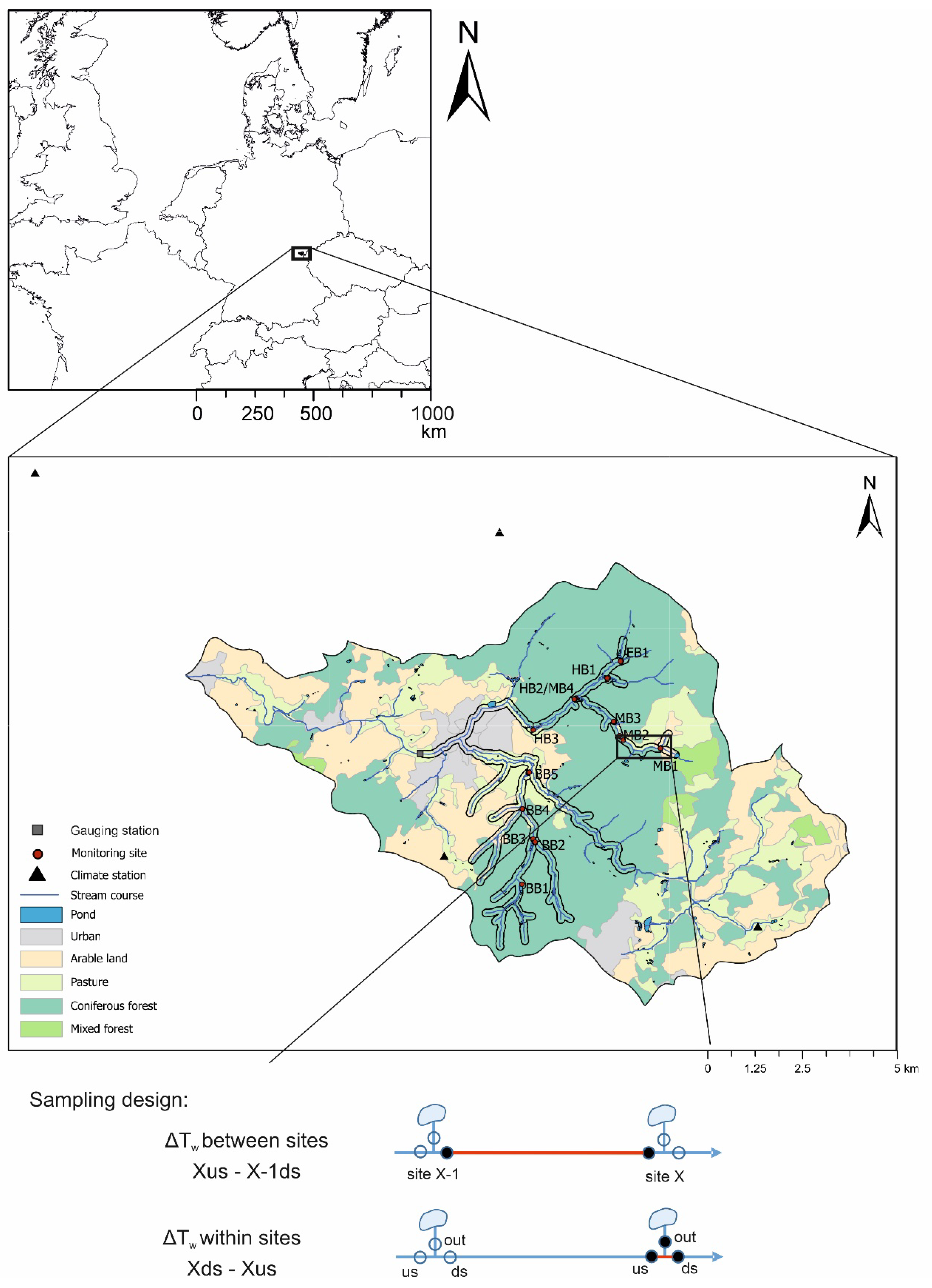
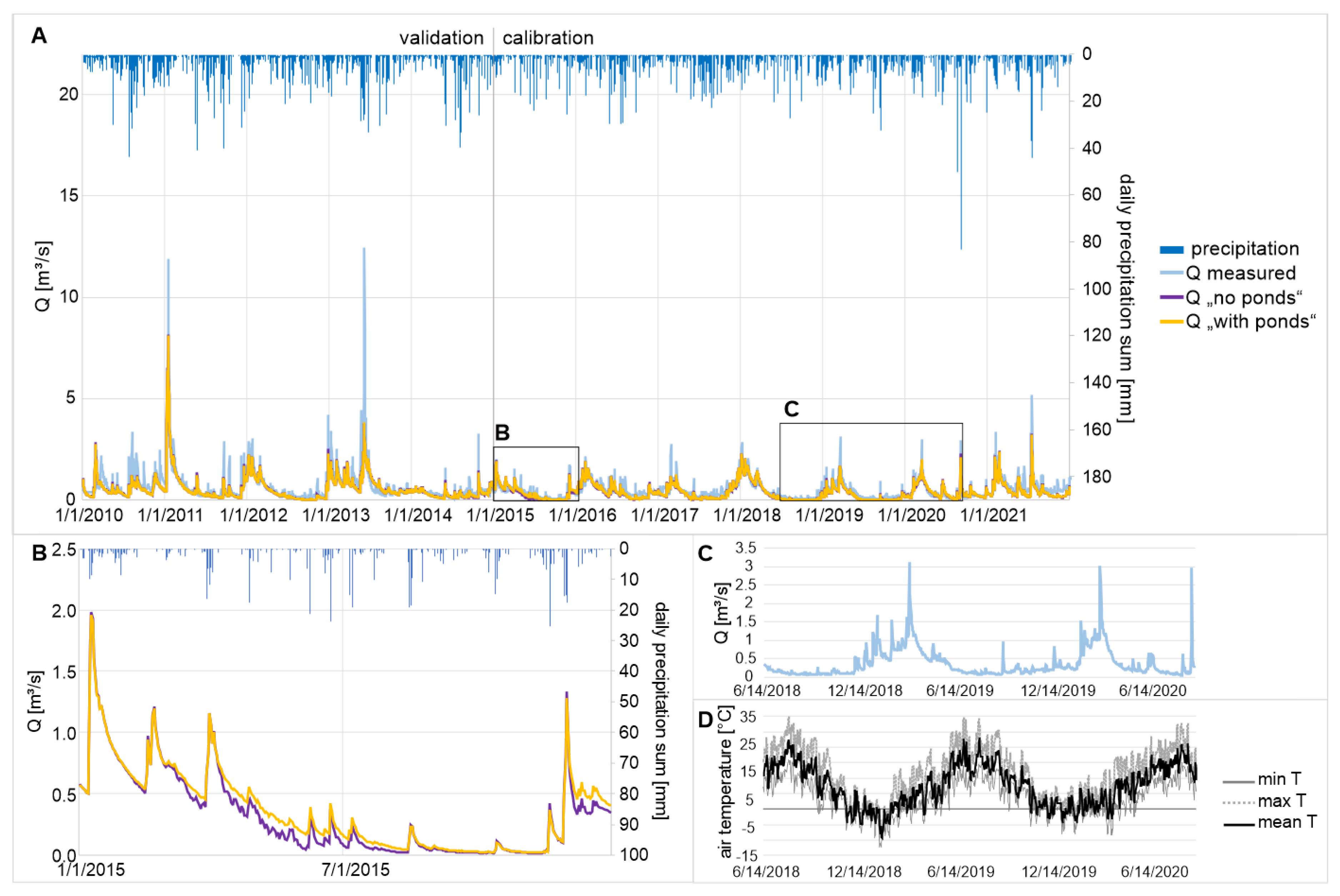
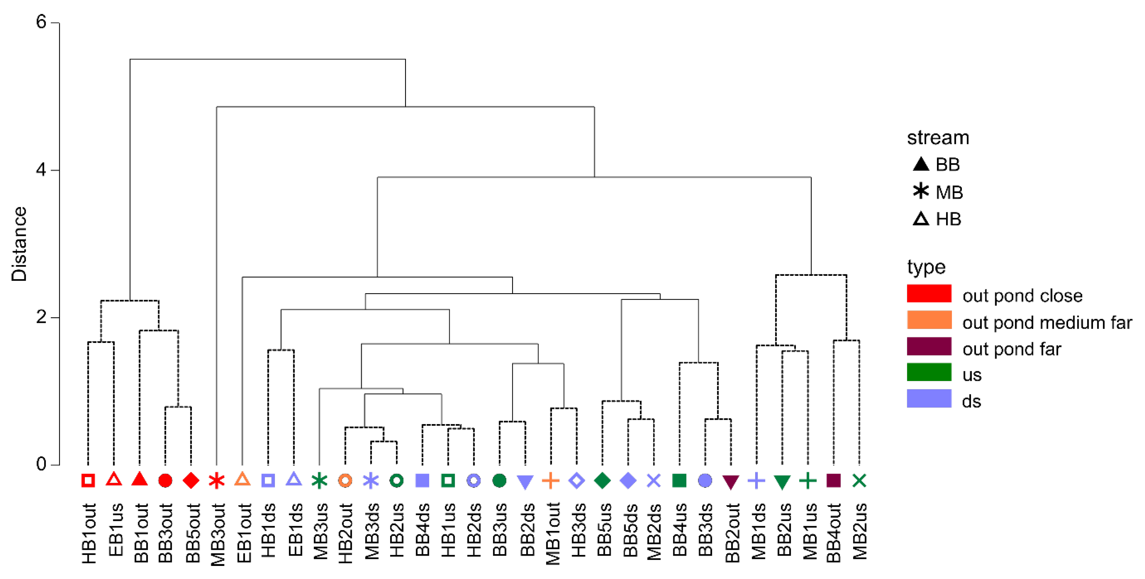
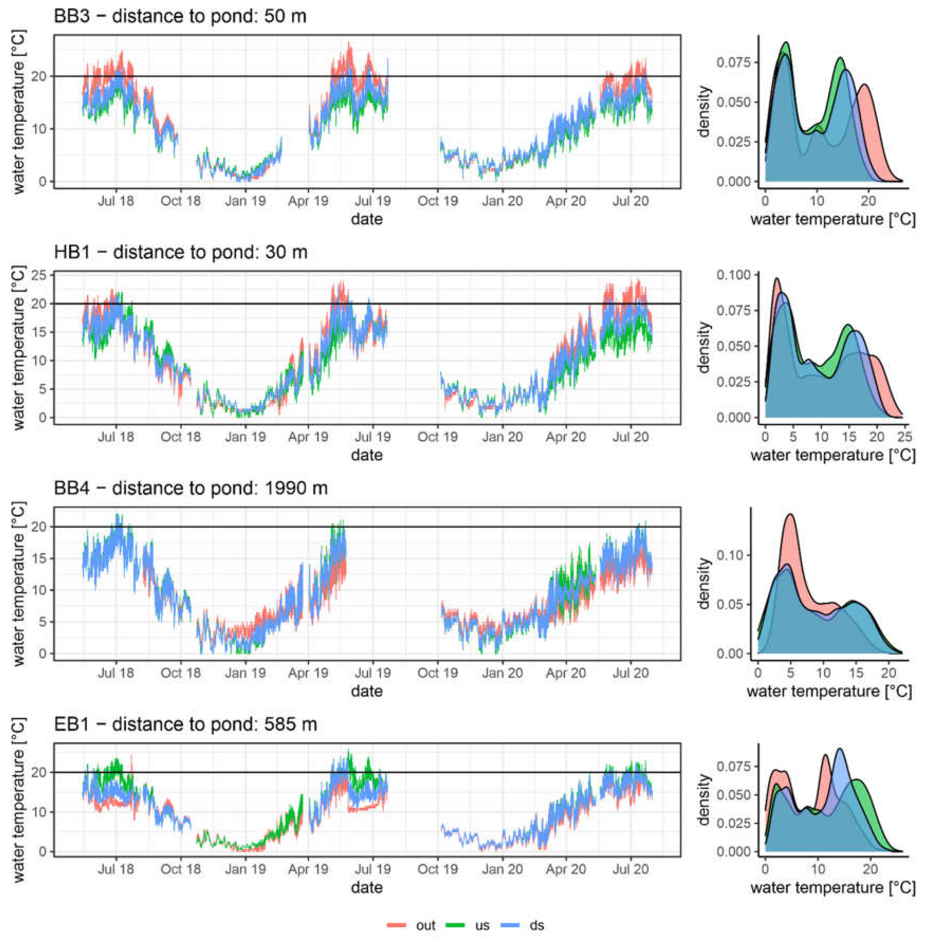
Table 1.
Initial input variables used to integrate ponds into the SWAT model: PND-parameters, definition and source.
Table 1.
Initial input variables used to integrate ponds into the SWAT model: PND-parameters, definition and source.
| Parameter | Definition | Source |
|---|---|---|
| PND_FR | Fraction of subbasin area that drains into ponds (0–1) | DEM |
| PND_PSA | Surface area of ponds when filled to principal spillway [ha] | Shape file based on orthophotos |
| PND_PVOL | Volume of water stored in ponds when filled to the principal spillway [104 m3 H2O] | Surface area × depth (=0.8 m, mean depth derived from field observations) |
| PND_ESA | Surface area of ponds when filled to emergency spillway [ha] | PSA × 1.1 (derived from field observations) |
| PND_EVOL | Volume of water stored in ponds when filled to the emergency spillway [104 m3 H2O] | PSA × depth (=1.0 m, derived from field observations) |
| PND_VOL | Initial volume of water in ponds [104 m3 H2O] | =PVOL |
| PND_SED | Initial sediment concentration in pond water [mg/L] | 39 (derived from water samples from fish-free pond) |
| PND_NSED | Equilibrium sediment concentration in pond water [mg/L] | 96 (derived from water samples from stocked pond) |
| PND_K | Hydraulic conductivity through the bottom of ponds (mm/h) | 1 (after Baldan et al. [67]) |
| IFLOD1 | Beginning month of non-flood season | 0 |
| IFLOD 2 | Ending month of non-flood season | 0 |
| NDTARG | Number of days needed to reach target storage from current pond storage [d] | 5 (derived from field observations) |
| PND_D50 | Median particle diameter of sediment [µm] | 10 (default) |
Table 2.
Parameters used in the calibration with SWAT CUP, their initial calibration range and the value fitted after calibration, small letter before the parameters represents the mode of adapting the parameter during the calibration (r = relative, v = replace, a = add).
Table 2.
Parameters used in the calibration with SWAT CUP, their initial calibration range and the value fitted after calibration, small letter before the parameters represents the mode of adapting the parameter during the calibration (r = relative, v = replace, a = add).
| Parameter | Definition | Initial Calibration Range | Fitted Value |
|---|---|---|---|
| r__CN2.mgt | Initial SCS runoff curve number for soil moisture condition II | −0.5–0.5 | −0.302425 |
| v__ESCO.hru | Soil evaporation compensation factor of HRU | 0.0–0.5 | −0.207090 |
| r_SOL_AWC(#).sol | Available water capacity of the soil layer (#) (mm H2O/mm soil) | −1.0–0.5 | −0.404389 |
| r__SOL_BD(#).sol | Moist bulk density of the soil layer (#) (mg/m3) | 0.0–0.7 | 0.640855 |
| a__CANMX.hru | Maximum canopy storage (mm H2O) | 80–180 | 82.587418 |
| r__SOL_K(#).sol | Saturated hydraulic conductivity of the soil layer (#) (mm/h) | −0.2–0.8 | 0.755521 |
| a__GW_REVAP.gw | Groundwater “revap” coefficient | 0.00–0.18 | 0.061701 |
| a__GWQMN.gw | Threshold depth of water in the shallow aquifer required for return flow to occur (mm H2O) | −1000–2000 | −500.878265 |
| a__REVAPMN.gw | Threshold depth of water in the shallow aquifer required for “revap” or percolation to the deep aquifer to occur (mm H2O) | −750–0 | −373.519958 |
| r__SLSUBBSN.hru | Average slope length (m) | −0.5–1.0 | 0.580487 |
| a__GW_DELAY.gw | Groundwater delay time (days) | 100–350 | 41.244041 |
| a__OV_N.hru | Manning’s “n” for overland flow | 0–100 | 47.643097 |
| v__PND_K.pnd | Hydraulic conductivity through bottom of ponds (mm/h) | 0–1 | 0.602785 |
| v__ALPHA_BF.gw | Baseflow alpha factor (1/days) | 0–1 | 0.799400 |
| v__RCHRG_DP.gw | Deep aquifer percolation fraction | 0.0–0.4 | 0.231797 |
Table 3.
Temperature metrics used to describe the thermal regime at the monitoring points, and their ecological relevance.
Table 3.
Temperature metrics used to describe the thermal regime at the monitoring points, and their ecological relevance.
| Metrics | Relevance | |
|---|---|---|
| Magnitude | ||
| ADM_su | Average daily mean Tw in summer | Physiological response, development/growth rates, concept of degree-days |
| ADM_wi | Average daily mean Tw in winter | |
| MaxD_su | Maximum daily mean Tw in summer | Potential thermal limit for aquatic organisms |
| MaxD_wi | Maximum daily mean Tw in winter | |
| AMax_su | Average daily maximum Tw in summer | |
| AMax_wi | Average daily maximum Tw in winter | |
| MaxT | Maximum daily maximum Tw in summer | |
| Variability | ||
| Range_su | Average daily range in Tw in summer | Dial variation |
| Range_wi | Average daily range in Tw in winter | |
| Timing | ||
| Jdmax | Julian day of MaxT in summer | Possible shift in timing of life history transitions |
| Frequency | ||
| b14_5 | Number of days in summer with average daily Tw < 14.5 °C | Tw > 14.5 °C needed to achieve sufficient growth in FPM |
| a20 | Number of days in summer with maximum daily Tw > 20 °C | Host fish (brown trout) will migrate from stream reach at Tw > 21 °C |
Table 4.
Calibration output; classification of evaluation parameters after Moriasi et al. [75] for daily stream flow data at subbasin 32.
Table 4.
Calibration output; classification of evaluation parameters after Moriasi et al. [75] for daily stream flow data at subbasin 32.
| NSE | PBIAS | R2 | |
|---|---|---|---|
| Calibration 1 January 2015–31 December 2021 | 0.71 “good” | 3.3 “very good” | 0.71 “good” |
| Validation 1 January 2010–31 December 2014 | 0.77 “good” | 16.2 “not satisfactory” | 0.79 “good” |
Table 5.
Average temperature metrics (codes after Table 3, su = summer, wi = winter) at the three monitoring points per site, as well as the difference between the value calculated at ‘us’ compared to ‘ds’ (delta value) over the whole study period.
Table 5.
Average temperature metrics (codes after Table 3, su = summer, wi = winter) at the three monitoring points per site, as well as the difference between the value calculated at ‘us’ compared to ‘ds’ (delta value) over the whole study period.
| ADM [°C] | MaxD [°C] | Amax [°C] | Range [°C] | MaxT [°C] | Jdmax | b14_5 | a20 | |||||
|---|---|---|---|---|---|---|---|---|---|---|---|---|
| su | wi | su | wi | su | wi | su | wi | su | su | su | su | |
| BB1 | 19.2 | 4.4 | 22.5 | 6.7 | 20.2 | 4.6 | 1.9 | 0.5 | 23.8 | 218 | 4.0 | 44.0 |
| BB2 out | 15.9 | 2.9 | 20.1 | 5.9 | 17.6 | 3.4 | 3.2 | 1.0 | 22.3 | 209 | 17.7 | 7.7 |
| BB2 us | 13.5 | 3.0 | 16.5 | 5.6 | 14.9 | 3.5 | 2.6 | 0.9 | 17.8 | 207 | 62.0 | 0.0 |
| BB2 ds | 14.8 | 3.2 | 18.4 | 5.6 | 16.2 | 3.5 | 2.7 | 0.7 | 20.5 | 204 | 35.3 | 2.0 |
| Delta BB2 | 1.3 | 0.1 | 1.9 | 0.0 | 1.3 | 0.0 | 0.0 | −0.1 | 2.7 | −4 | −26.7 | 2.0 |
| BB3 out | 19.2 | 2.4 | 22.8 | 5.0 | 20.6 | 2.6 | 2.7 | 0.4 | 25.0 | 211 | 2.3 | 47.0 |
| BB3 us | 14.9 | 2.9 | 18.6 | 5.9 | 16.4 | 3.4 | 2.9 | 1.0 | 20.7 | 208 | 33.7 | 1.0 |
| BB3 ds | 16.2 | 2.8 | 19.5 | 5.6 | 17.8 | 3.3 | 3.0 | 0.9 | 22.2 | 229 | 15.7 | 10.3 |
| Delta BB3 | 1.3 | −0.1 | 0.9 | −0.2 | 1.4 | −0.1 | 0.1 | −0.1 | 1.5 | 22 | −18.0 | 9.3 |
| BB4 out | 13.4 | 4.2 | 16.3 | 6.4 | 15.7 | 4.9 | 4.1 | 1.4 | 19.5 | 229 | 65.0 | 0.0 |
| BB4 us | 15.9 | 2.7 | 19.3 | 6.0 | 17.8 | 3.5 | 3.8 | 1.4 | 22.2 | 226 | 19.3 | 11.3 |
| BB4 ds | 15.6 | 3.0 | 19.0 | 6.0 | 17.4 | 3.7 | 3.5 | 1.4 | 21.7 | 205 | 23.0 | 6.7 |
| Delta BB4 | −0.3 | 0.2 | −0.3 | 0.0 | −0.4 | 0.2 | −0.3 | 0.0 | −0.5 | −22 | 3.7 | −4.7 |
| BB5 out | 19.0 | 3.1 | 23.5 | 5.7 | 20.3 | 3.4 | 2.7 | 0.6 | 25.7 | 205 | 4.3 | 41.3 |
| BB5 us | 15.9 | 3.0 | 19.5 | 6.3 | 18.2 | 3.9 | 4.2 | 1.6 | 22.5 | 204 | 19.7 | 14.3 |
| BB5 ds | 16.3 | 3.0 | 19.9 | 6.1 | 18.5 | 3.8 | 4.1 | 1.5 | 23.2 | 211 | 16.7 | 18.3 |
| Delta BB5 | 0.4 | 0.0 | 0.5 | −0.1 | 0.3 | 0.0 | −0.1 | −0.1 | 0.7 | 7 | −3.0 | 4.0 |
| MB1 out | 15.6 | 2.7 | 19.1 | 5.1 | 17.2 | 3.3 | 3.0 | 1.0 | 21.0 | 215 | 27.0 | 3.0 |
| MB1 us | 12.6 | 3.5 | 15.9 | 6.2 | 14.2 | 4.3 | 3.1 | 1.5 | 17.5 | 218 | 74.0 | 0.0 |
| MB1 ds | 13.6 | 3.3 | 17.0 | 5.9 | 15.1 | 4.0 | 3.1 | 1.3 | 19.2 | 224 | 60.7 | 0.3 |
| Delta MB1 | 1.0 | −0.1 | 1.5 | −0.2 | 0.9 | −0.2 | −0.1 | −0.2 | 1.0 | 3 | −13.5 | 0.0 |
| MB2 us | 14.0 | 2.8 | 17.2 | 5.6 | 16.0 | 3.4 | 4.0 | 1.1 | 20.0 | 211 | 51.0 | 0.5 |
| MB2 ds | 15.8 | 3.0 | 19.7 | 5.8 | 18.1 | 3.7 | 4.3 | 1.3 | 23.5 | 214 | 20.7 | 15.7 |
| Delta MB2 | 2.2 | −0.2 | 3.0 | 0.0 | 2.8 | −0.1 | 0.6 | 0.1 | 4.5 | −2 | −37.5 | 20.5 |
| MB3 out | 15.8 | 1.9 | 19.4 | 5.4 | 17.2 | 2.5 | 2.6 | 1.1 | 23.0 | 154 | 21.0 | 8.0 |
| MB3 us | 15.3 | 2.5 | 18.9 | 5.8 | 17.4 | 3.2 | 4.1 | 1.3 | 21.5 | 204 | 27.7 | 7.3 |
| MB3 ds | 14.9 | 2.5 | 18.3 | 5.8 | 16.9 | 3.2 | 3.7 | 1.3 | 20.8 | 207 | 33.3 | 2.3 |
| Delta MB3 | −0.3 | 0.0 | −0.6 | 0.0 | −0.6 | 0.0 | −0.4 | 0.0 | −0.8 | 2 | 5.7 | −5.0 |
| EB1 out | 14.0 | 2.1 | 18.3 | 5.0 | 15.8 | 2.6 | 3.2 | 1.0 | 23.7 | 210 | 44.7 | 7.0 |
| EB1 us | 17.9 | 2.0 | 21.8 | 4.8 | 19.8 | 2.4 | 3.5 | 0.6 | 24.2 | 201 | 4.0 | 37.0 |
| EB1 ds | 15.8 | 2.7 | 19.9 | 5.0 | 17.7 | 3.2 | 3.3 | 1.0 | 22.3 | 186 | 23.7 | 14.0 |
| Delta EB1 | −2.1 | 0.0 | −1.9 | 0.0 | −2.1 | 0.0 | −0.2 | 0.0 | −1.8 | −15 | 19.7 | −23.0 |
| HB1 out | 18.0 | 2.1 | 22.0 | 4.8 | 19.5 | 2.4 | 3.0 | 0.5 | 24.3 | 220 | 8.7 | 35.7 |
| HB1 us | 15.3 | 2.5 | 18.7 | 5.7 | 17.1 | 3.0 | 3.5 | 1.0 | 21.0 | 206 | 27.0 | 6.0 |
| HB1 ds | 16.5 | 2.6 | 20.0 | 5.2 | 18.1 | 3.0 | 3.2 | 0.7 | 22.0 | 203 | 9.7 | 11.3 |
| Delta HB1 | 1.2 | 0.1 | 1.3 | −0.6 | 1.0 | −0.1 | −0.3 | −0.3 | 1.0 | −3 | −17.3 | 5.3 |
| HB2 out | 14.7 | 2.7 | 18.2 | 6.0 | 16.5 | 3.4 | 3.7 | 1.3 | 20.5 | 205 | 37.7 | 4.7 |
| HB2 us | 15.1 | 3.0 | 17.8 | 5.5 | 17.0 | 3.4 | 3.7 | 0.8 | 20.8 | 206 | 31.5 | 3.5 |
| HB2 ds | 15.5 | 2.7 | 18.7 | 5.7 | 17.3 | 3.2 | 3.7 | 1.1 | 20.8 | 204 | 22.3 | 5.7 |
| Delta HB2 | 0.8 | 0.2 | 1.0 | 0.4 | 0.6 | 0.2 | −0.1 | 0.1 | 0.3 | −5 | −15.5 | 3.0 |
| Delta MB4 | 0.8 | −0.1 | 0.5 | −0.2 | 0.8 | −0.1 | 0.0 | −0.1 | 0.3 | −1 | −15.3 | 1.0 |
| HB3 ds | 15.8 | 2.4 | 19.5 | 5.6 | 17.4 | 3.0 | 3.2 | 1.1 | 21.5 | 208 | 20.7 | 6.0 |
Table 6.
Proportion of different LU categories within the 180 m corridor along the reach between the subsequent monitoring points; reaches are differentiated between short stretches covering the distance between monitoring points upstream and downstream of a channel inflow (site X) and longer stretches covering the distance between two subsequent monitoring points (point X–point X + 1); within a sampling site, this refers to the reach between ‘us’ and ‘ds’ monitoring points; between sampling sites, this refers to the reach between ‘ds’ point of the upstream and ‘us’ point of the subsequent site.
| Reach | Reach Length (km) | % Pond Area | % Forested Area | % Open Land | Total Area [ha] |
|---|---|---|---|---|---|
| BB1 | 0.77 | 12.5 | 87.5 | 0.0 | 42.49 |
| BB1-BB2 | 1.44 | 0.8 | 99.2 | 0.0 | 71.58 |
| BB2 | 0.06 | 5.2 | 94.8 | 0.0 | 114.07 |
| BB2-BB3 | 0.11 | 0.0 | 100.0 | 0.0 | 1.34 |
| BB3 | 0.02 | 16.3 | 83.7 | 0.0 | 5.51 |
| BB3-BB4 | 1.16 | 0.0 | 68.1 | 31.9 | 16.39 |
| BB4 | 0.02 | 0.1 | 47.2 | 52.7 | 62.27 |
| BB4-BB5 | 1.16 | 0.8 | 5.0 | 94.2 | 34.44 |
| BB5 | 0.03 | 12.9 | 0.0 | 87.1 | 2.73 |
| EB1 | 0.02 | 3.3 | 96.7 | 0.0 | 3.62 |
| HB1 | 0.06 | 7.1 | 92.9 | 0.0 | 12.24 |
| HB1-HB2 | 1.18 | 2.6 | 97.4 | 0.0 | 32.43 |
| HB2 | 0.03 | 50.4 | 49.6 | 0.0 | 2.03 |
| HB2-HB3 | 1.75 | 2.3 | 47.8 | 40.0 | 34.38 |
| MB1 | 0.03 | 8.7 | 8.2 | 83.0 | 9.07 |
| MB1-MB2 | 1.16 | 0.3 | 59.8 | 40.0 | 22.86 |
| MB2 | 0.16 | 7.8 | 57.2 | 35.0 | 3.17 |
| MB2-MB3 | 0.39 | 0.0 | 68.2 | 31.8 | 6.63 |
| MB3 | 0.02 | 25.4 | 74.6 | 0.0 | 1.48 |
| MB3-MB4/HB2 | 1.35 | 2.6 | 97.4 | 0.0 | 26.39 |
Publisher’s Note: MDPI stays neutral with regard to jurisdictional claims in published maps and institutional affiliations. |
© 2022 by the authors. Licensee MDPI, Basel, Switzerland. This article is an open access article distributed under the terms and conditions of the Creative Commons Attribution (CC BY) license (https://creativecommons.org/licenses/by/4.0/).
Share and Cite
MDPI and ACS Style
Hoess, R.; Generali, K.A.; Kuhn, J.; Geist, J. Impact of Fish Ponds on Stream Hydrology and Temperature Regime in the Context of Freshwater Pearl Mussel Conservation. Water 2022, 14, 2490. https://doi.org/10.3390/w14162490
AMA Style
Hoess R, Generali KA, Kuhn J, Geist J. Impact of Fish Ponds on Stream Hydrology and Temperature Regime in the Context of Freshwater Pearl Mussel Conservation. Water. 2022; 14(16):2490. https://doi.org/10.3390/w14162490
Chicago/Turabian StyleHoess, Rebecca, Konstantina A. Generali, Johannes Kuhn, and Juergen Geist. 2022. "Impact of Fish Ponds on Stream Hydrology and Temperature Regime in the Context of Freshwater Pearl Mussel Conservation" Water 14, no. 16: 2490. https://doi.org/10.3390/w14162490
Note that from the first issue of 2016, this journal uses article numbers instead of page numbers. See further details here.