
A Stepwise Modelling Approach to Identifying Structural Features That Control Groundwater Flow in a Folded Carbonate Aquifer System

 , , , and
Abstract
:1. Introduction
2. Conceptual Model
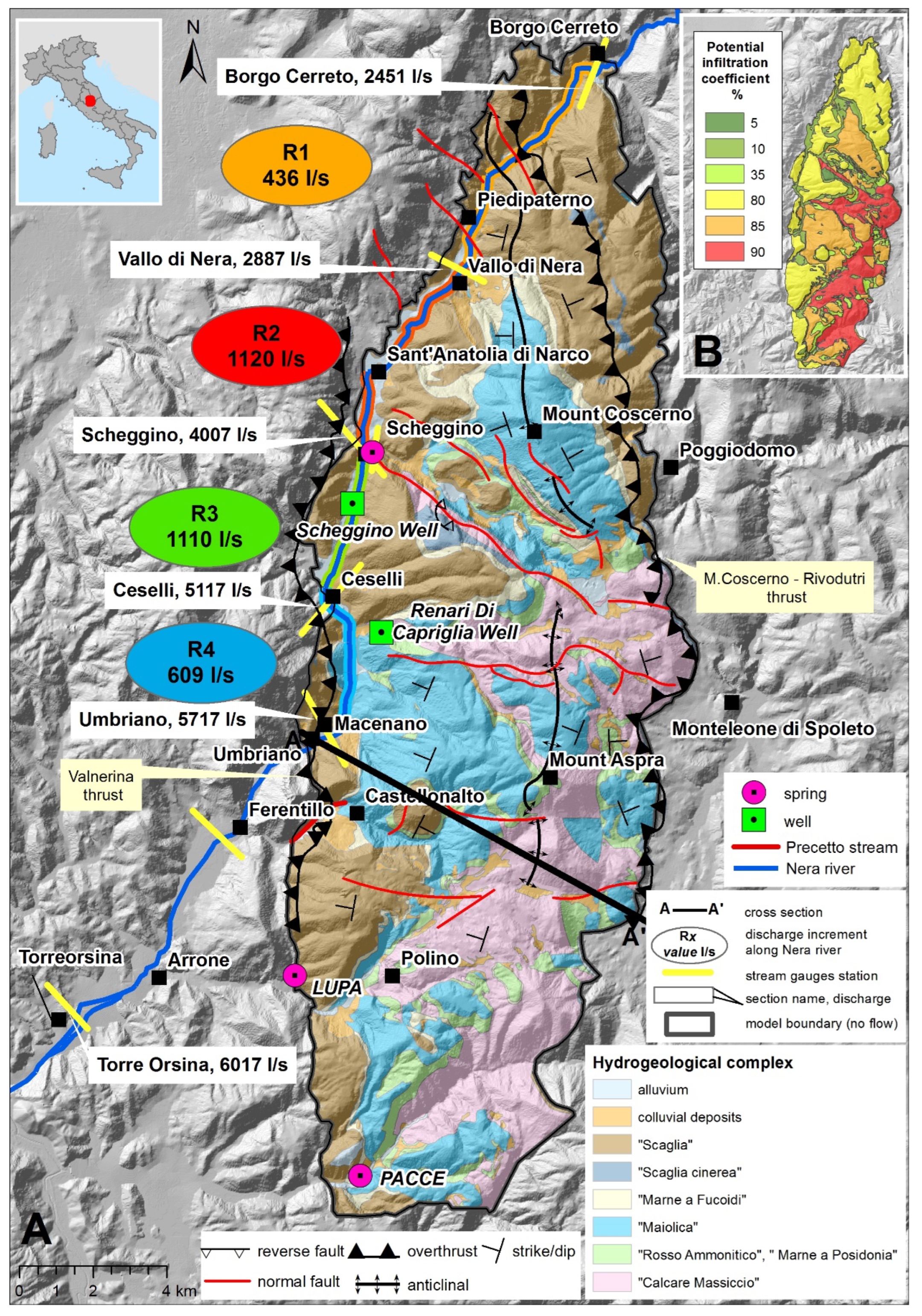
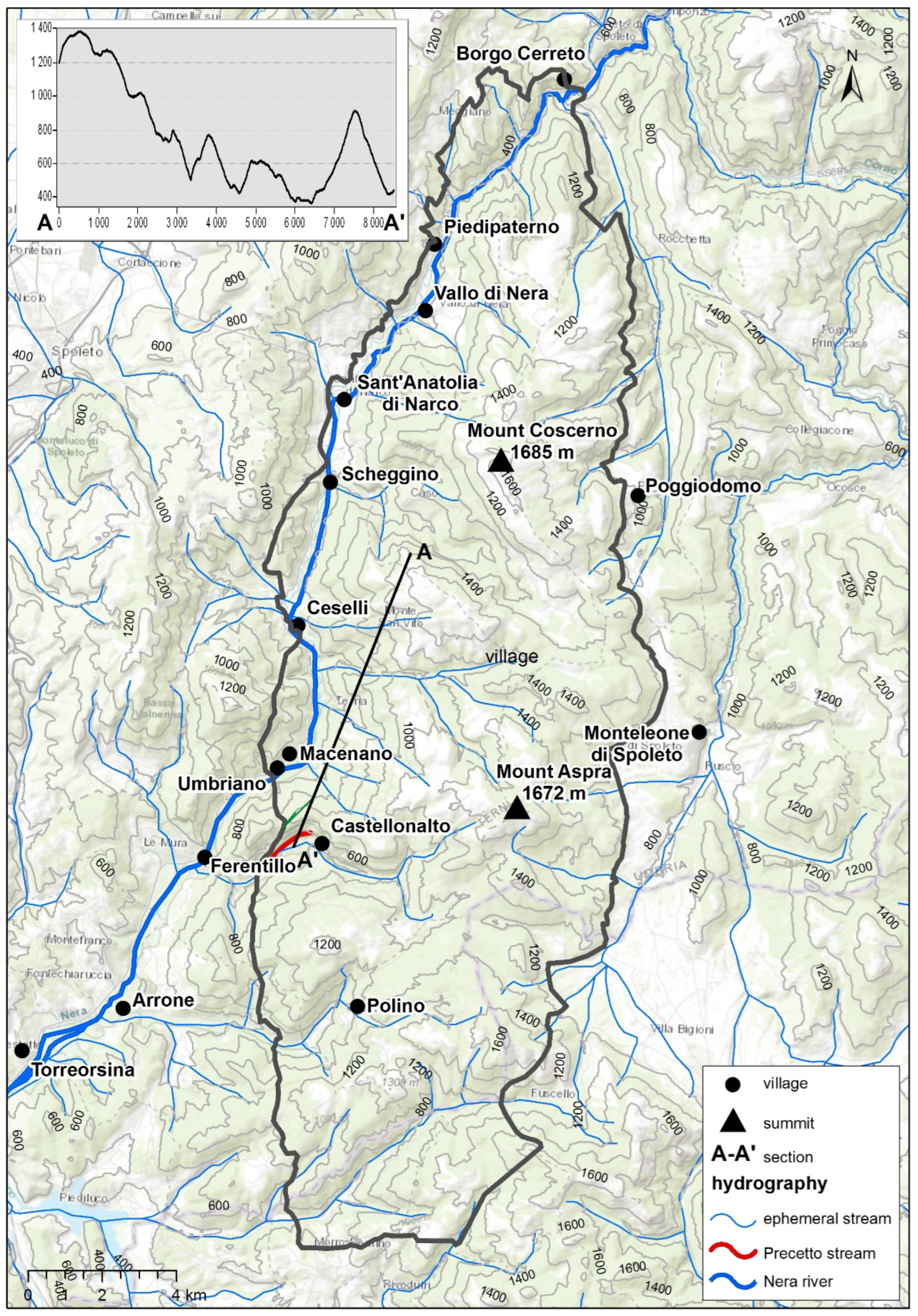
2.1. Geological and Hydrogeological Setting
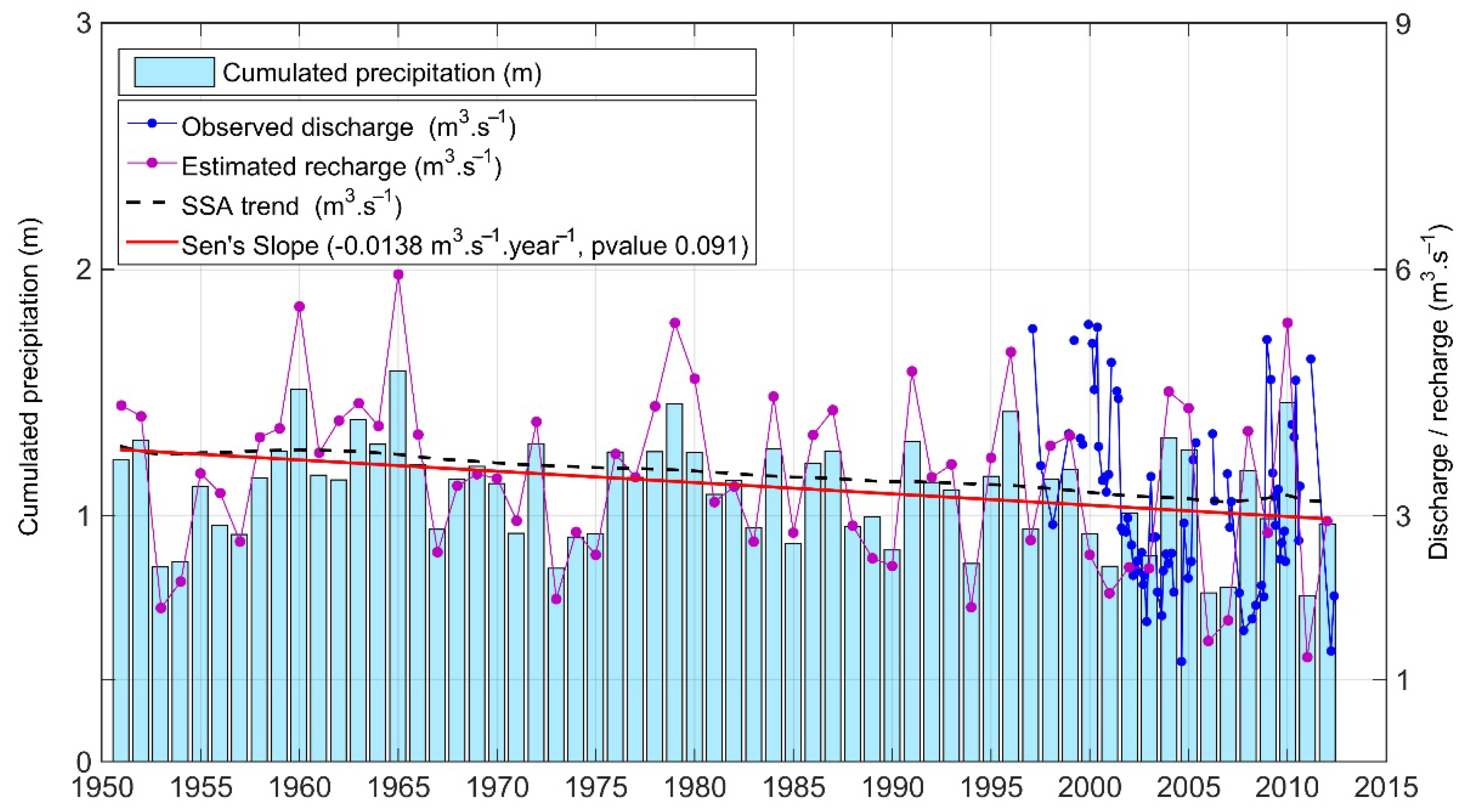
2.2. Recharge Estimation
3. Numerical Model Description
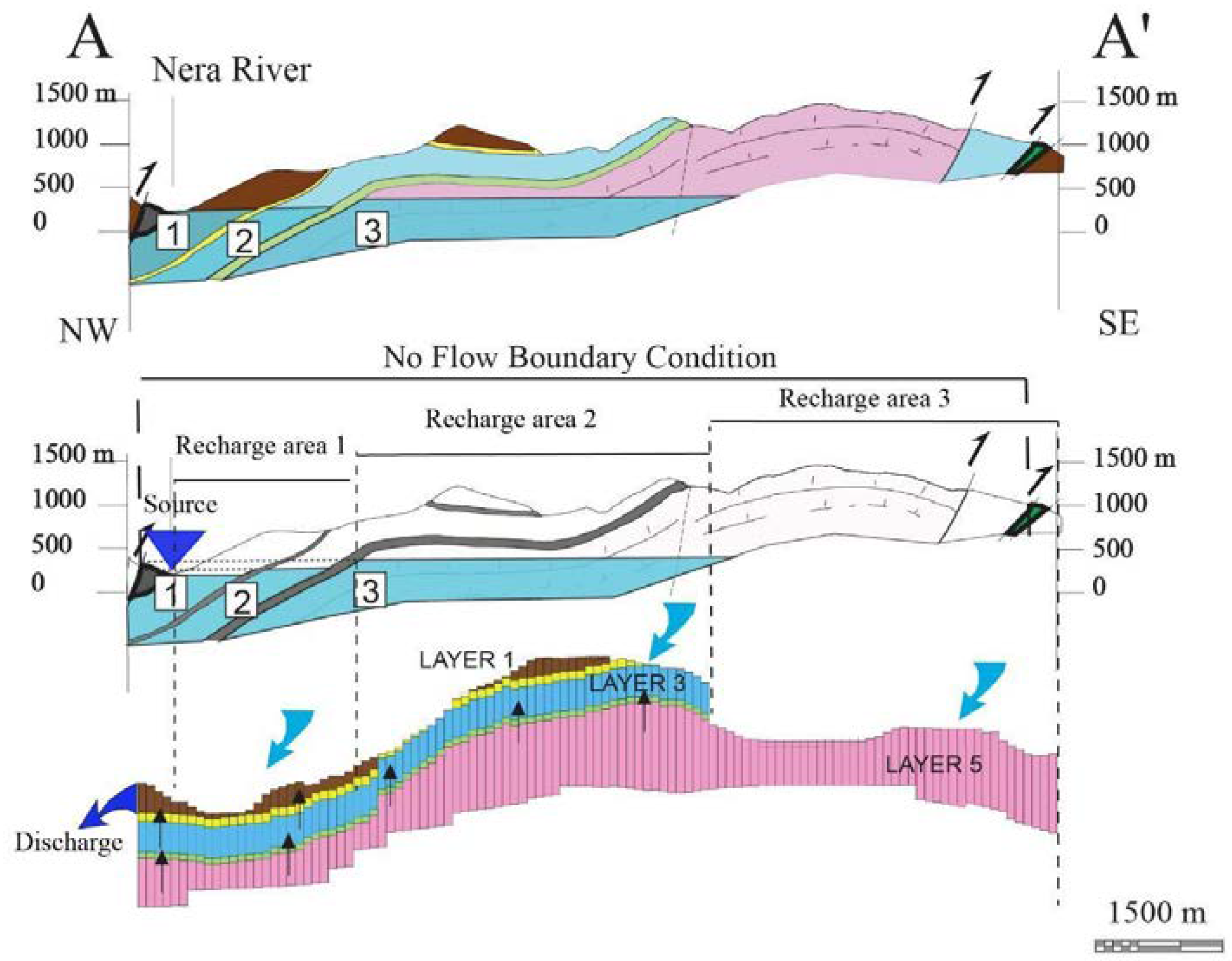
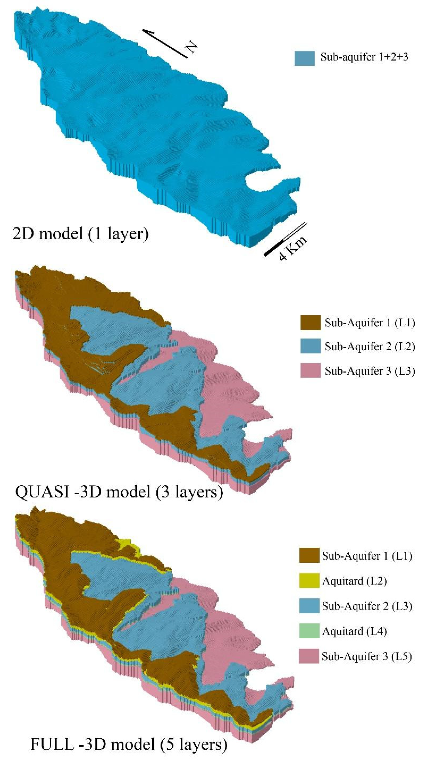
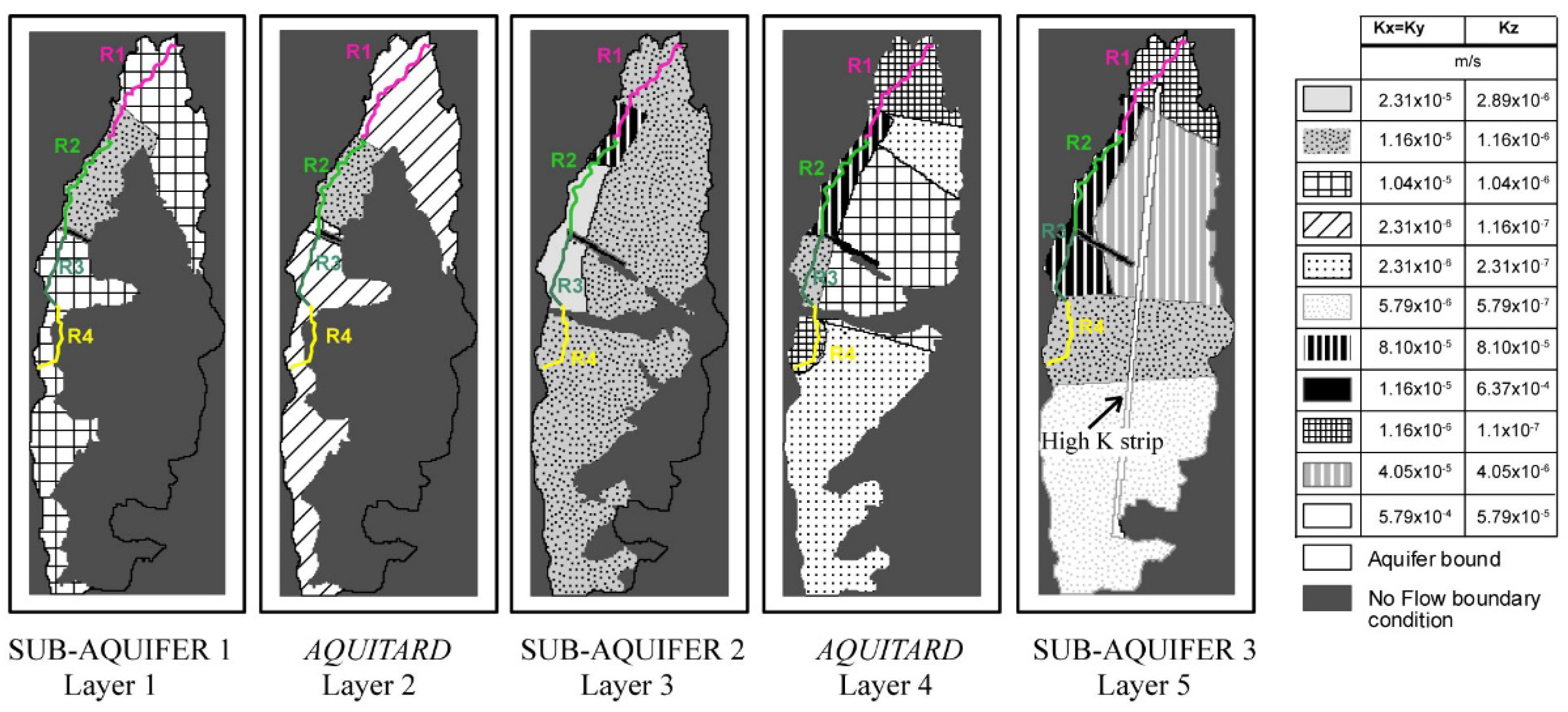
3.1. Layers Discretization, Boundary Conditions and Codes
- T1, T2, T3, T4, T5 = transmissivity of the fully 3D model (subscript indicates the layer)
- T1′, T2′, T3′ = transmissivity of the quasi-3D model (subscript indicates the layer)
- T2D = transmissivity of the 2D model
- Kn = permeability (subscript indicates the layer)
- en = thickness (subscript indicates the layer)
3.2. Model Calibration
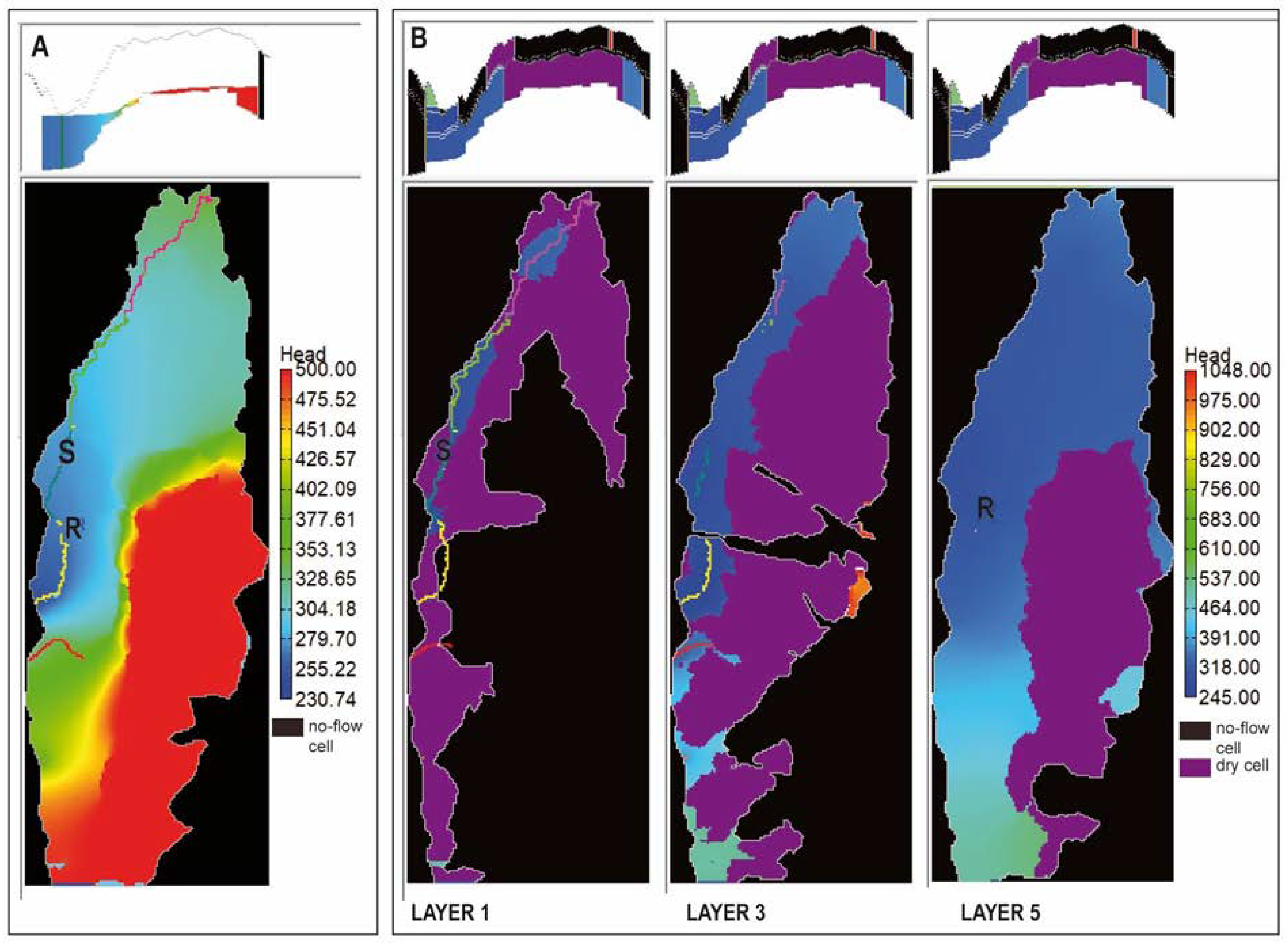
4. Results and Discussion
5. Conclusions
Author Contributions
Funding
Data Availability Statement
Acknowledgments
Conflicts of Interest
References
- Ford, D.C.; Williams, P.W. Karst Hydrogeology and Geomorphology; John Wiley & Sons: Chichester, UK; Hoboken, NJ, USA, 2007. [Google Scholar]
- Worthington, S.; Ford, D. Self-Organized Permeability in Carbonate Aquifers. Ground Water 2009, 47, 326–336. [Google Scholar] [CrossRef] [PubMed]
- Worthington, S.R.H. Management of Carbonate Aquifers. In Karst Management; Van Beynen, P.E., Ed.; Department Geography, University of South Florida: Tampa, FL, USA, 2011; Volume XII, pp. 243–261. [Google Scholar] [CrossRef]
- Dragoni, W.; Mottola, A.; Cambi, C. Modeling the effects of pumping wells in spring management: The case of Scirca spring (central Apennines, Italy). J. Hydrol. 2013, 493, 115–123. [Google Scholar] [CrossRef]
- Fiorillo, F.; Guadagno, F.M. Karst Spring Discharges Analysis in Relation to Drought Periods, Using the SPI. Water Resour. Manag. 2010, 24, 1867–1884. [Google Scholar] [CrossRef]
- Romano, E.; Preziosi, E. Precipitation pattern analysis in the Tiber River basin (central Italy) using standardized indices. Int. J. Climatol. 2013, 33, 1781–1792. [Google Scholar] [CrossRef]
- Citrini, A.; Camera, C.; Beretta, G.P. Nossana Spring (Northern Italy) under Climate Change: Projections of Future Discharge Rates and Water Availability. Water 2020, 12, 387. [Google Scholar] [CrossRef]
- Leone, G.; Pagnozzi, M.; Catani, V.; Ventafridda, G.; Esposito, L.; Fiorillo, F. A hundred years of Caposele spring discharge measurements: Trends and statistics for understanding water resource availability under climate change. Stoch. Hydrol. Hydraul. 2020, 35, 345–370. [Google Scholar] [CrossRef]
- Romano, E.; Petrangeli, A.B.; Salerno, F.; Guyennon, N. Do recent meteorological drought events in central Italy result from long-term trend or increasing variability? Int. J. Clim. 2021, 42, 4111–4128. [Google Scholar] [CrossRef]
- Romano, E.; Petrangeli, A.B.; Preziosi, E. Spati al and Time Analysis of Rainfall in the Tiber River Basin (Central Italy) in relation to Discharge Measurements (1920-2010). Procedia Environ. Sci. 2011, 7, 258–263. [Google Scholar] [CrossRef]
- IPCC 2022—Climate Change 2022: Impacts, Adaptation, and Vulnerability. Contribution of Working Group II to the Sixth Assessment Report of the Intergovernmental Panel on Climate Change; Pörtner, H.-O.; Roberts, D.C.; Tignor, M.; Poloczanska, E.S.; Mintenbeck, K.; Alegría, A.; Craig, M.; Langsdorf, S.; Löschke, S.; Möller, V.; et al. (Eds.) Cambridge University Press: Cambridge, UK, 2022. [Google Scholar]
- Preziosi, E.; Romano, E. Are large karstic springs good indicators for Climate Change effects on groundwater? In Proceedings of the European Geosciences Union General Assembly 2013, Vienna, Austria, 7–12 April 2013. Geophys. Res. Abstr. 2013, 15, 9367. [Google Scholar]
- Romano, E.; Del Bon, A.; Petrangeli, A.; Preziosi, E. Generating synthetic time series of springs discharge in relation to standardized precipitation indices. Case study in Central Italy. J. Hydrol. 2013, 507, 86–99. [Google Scholar] [CrossRef]
- Band, S.S.; Heggy, E.; Bateni, S.M.; Karami, H.; Rabiee, M.; Samadianfard, S.; Chau, K.-W.; Mosavi, A. Groundwater level prediction in arid areas using wavelet analysis and Gaussian process regression. Eng. Appl. Comput. Fluid Mech. 2021, 15, 1147–1158. [Google Scholar] [CrossRef]
- Mallick, J.; Almesfer, M.K.; Alsubih, M.; Talukdar, S.; Ahmed, M.; Kahla, N.B. Developing a new method for future groundwater potentiality mapping under climate change in Bisha watershed, Saudi Arabia. Geocarto Int. 2022, 1, 1–33. [Google Scholar] [CrossRef]
- Snoussi, M.; Jerbi, H.; Tarhouni, J. Integrated Groundwater Flow Modeling for Managing a Complex Alluvial Aquifer Case of Study Mio-Plio-Quaternary Plain of Kairouan (Central Tunisia). Water 2022, 14, 668. [Google Scholar] [CrossRef]
- European Community. Directive 2000/60/EC of the European Parliament and of the Council of 23 October 2000 Establishing a Framework for Community Action in the Field of Water Policy. 2000. Available online: https://eur-lex.europa.eu/LexUriServ/LexUriServ.do?uri=CELEX:32000L0060:EN:HTML (accessed on 5 July 2022).
- Gattinoni, P.; Francani, V. Depletion risk assessment of the Nossana Spring (Bergamo, Italy) based on the stochastic modeling of recharge. Appl. Hydrogeol. 2010, 18, 325–337. [Google Scholar] [CrossRef]
- Levison, J.; Larocque, M.; Ouellet, M. Modeling low-flow bedrock springs providing ecological habitats with climate change scenarios. J. Hydrol. 2014, 515, 16–28. [Google Scholar] [CrossRef]
- Reimann, T.; Giese, M.; Geyer, T.; Liedl, R.; Maréchal, J.C.; Shoemaker, W.B. Representation of water abstraction from a karst conduit with numerical discrete-continuum models. Hydrol. Earth Syst. Sci. 2014, 18, 227–241. [Google Scholar] [CrossRef]
- Scanlon, B.R.; Mace, R.E.; Barrett, M.E.; Smith, B. Can we simulate regional groundwater flow in a karst system using equivalent porous media models? Case study, Barton Springs Edwards aquifer, USA. J. Hydrol. 2003, 276, 137–158. [Google Scholar] [CrossRef]
- Abusaada, M.; Sauter, M. Studying the Flow Dynamics of a Karst Aquifer System with an Equivalent Porous Medium Model. Ground Water 2012, 51, 641–650. [Google Scholar] [CrossRef]
- Ben-Itzhak, L.; Gvirtzman, H. Groundwater flow along and across structural folding: An example from the Judean Desert, Israel. J. Hydrol. 2005, 312, 51–69. [Google Scholar] [CrossRef]
- Dafny, E.; Burg, A.; Gvirtzman, H. Effects of Karst and geological structure on groundwater flow: The case of Yarqon-Taninim Aquifer, Israel. J. Hydrol. 2010, 389, 260–275. [Google Scholar] [CrossRef]
- Valota, G.; Giudici, M.; Parravicini, G.; Ponzini, G.; Romano, E. Is the forward problem of ground water hydrology always well posed? Ground Water 2002, 40, 500–508. [Google Scholar] [CrossRef] [PubMed]
- Niswonger, R.G.; Panday, S.; Ibaraki, M. MODFLOW-NWT, A Newton formulation for MODFLOW-2005. US Geol. Surv. Tech. Methods 2011, 6, 44. [Google Scholar]
- Mantoglou, A. On optimal model complexity in inverse modeling of heterogeneous aquifers. J. Hydraul. Res. 2005, 43, 574–583. [Google Scholar] [CrossRef]
- Hill, M.C. The practical use of simplicity in developing groundwater models. Ground Water 2006, 44, 775–781. [Google Scholar] [CrossRef] [PubMed]
- Moore, C.; Wöhling, T.; Doherty, J. Efficient regularization and uncertainty analysis using a global optimization methodology. Water Resour. Res. 2010, 46, W08527. [Google Scholar] [CrossRef]
- Hill, M.C. Methods and Guidelines for Effective Model Calibration. In U.S. Geological Survey, Water-Resources Investigations Report 98–4005; U.S. Geological Survey: Denver, CO, USA, 1998; p. 98. Available online: https://water.usgs.gov/nrp/gwsoftware/modflow2000/WRIR98-4005.pdf (accessed on 10 August 2022).
- Barchi, M.R.; Lemmi, M. Geology of the area of Monte Coscerno-Monte di Civitella (South-eastern Umbria). Boll. Soc. Geol. Ital. 1996, 115, 601–624. [Google Scholar]
- Tavarnelli, E. Analisi geometrica e cinematica dei sovrascorrimenti compresi fra la Valnerina e la conca di Rieti (Appennino Umbro-Marchigiano-Sabino). Boll. Soc. Geol. Ital. 1996, 113, 249–259. [Google Scholar]
- Pace, P.; Calamita, F.; Tavarnelli, E. Brittle-Ductile Shear Zones along Inversion-Related Frontal and Oblique Thrust Ramps: Insights from the Central-Northern Apennines Curved Thrust System (Italy). In Ductile Shear Zones: From Micro- to Macro-Scales; Mukherjee, S., Mulchrone, K.F., Eds.; John Wiley & Sons: Chichester, UK, 2015; Chapter 8; pp. 111–127. [Google Scholar]
- Calamita, F.; Deiana, G. The arcuate shape of the Umbria-Marche-Sabina Apennines (central Italy). Tectonophysics 1988, 146, 139–147. [Google Scholar] [CrossRef]
- Boni, C.; Preziosi, E. Una possibile simulazione numerica dell’acquifero basale di M.Coscerno—M.Aspra (bacino del fiume Nera). Geol. Appl. E Idrogeol. 1993, 28, 131–140. [Google Scholar]
- Preziosi, E. Simulazioni Numeriche di Acquiferi Carbonatici in Aree Corrugate: Applicazioni al Sistema Idrogeologico Della Valnerina (Italia Centrale). In Quad IRSA-CNR; Istituto di Ricerca Sulle Acque-CNR: Rome, Italy, 2007; Volume 125, p. 225. ISSN 0390-6329. [Google Scholar]
- Mastrorillo, L.; Baldoni, T.; Banzato, F.; Boscherini, A.; Cascone, D.; Checcucci, R.; Petitta, M.; Boni, C. Quantitative hydrogeological analysis of the carbonate domain of the Umbria Region (Central Italy). Ital. J. Eng. Geol. Environ. 2009, 1, 137–155. [Google Scholar] [CrossRef]
- Mastrorillo, L.; Petitta, M. Hydrogeological conceptual model of the upper Chienti River Basin aquifers (Umbria-Marche Apennines). Ital. J. Geosci. 2014, 133, 396–408. [Google Scholar] [CrossRef]
- Di Matteo, L.; Dragoni, W.; Ulderico, V.; Latini, M.; Spinsanti, R. Risorse idriche sotterranee e loro gestione: Il caso dell’ATO2 Umbria (Umbria meridionale). Acque Sotter. 2005, 96, 9–21. [Google Scholar]
- Damiani, A.V.; Baldanza, A.; Barchi, M.R.; Boscherini, A.; Checcucci, R.; Decandia, F.A.; Felicioni, G.; Lemmi, M.; Luchetti, L.; Motti, A.; et al. Geological Map of Italy. Scale 1:50,000. Scheet 563 “Spoleto”; ISPRA-Servizio Geologico Nazionale: Roma, Italy, 2008. [Google Scholar]
- ARPA Umbria. Available online: https://apps.arpa.umbria.it/acqua/contenuto/monitoraggio-in-continuo-acque-sotterranee (accessed on 13 June 2022).
- Preziosi, E.; Romano, E. From hydrostructural analysis to mathematical modelling of regional aquifers. Ital. J. Eng. Geol. Environ. 2009, 1, 183–198. [Google Scholar] [CrossRef]
- ARPA Umbria. Il Sistema Informativo di Arpa Umbria e la Conoscenza Ambientale, a cura di Mauro Emiliano, Quaderni Arpa Umbria. 2004. Available online: https://www.arpa.umbria.it/pagine/il-sistema-informativo-di-arpa-umbria-e-la-conosce (accessed on 5 July 2022).
- White, W.B. Geomorphology and Hydrology of Karst Terrains; Oxford Universuty Press: New York, NY, USA, 1988; p. 464. [Google Scholar]
- Vigna, B.; Banzato, C. The hydrogeology of high-mountain carbonate areas: An example of some Alpine systems in southern Piedmont (Italy). Environ. Earth Sci. 2015, 74, 267–280. [Google Scholar] [CrossRef]
- Thornthwaite, C.W.; Mather, J.R. The water balance. Climatology 1955, 8, 5–86. [Google Scholar]
- Thornthwaite, C.W.; Mather, J.R. Instructions and Tables for Computing Potential Evapotranspiration and the Water Balance. Centerton 1957, 10, 185–310. [Google Scholar]
- Umbriadue Servizi Idrici S.C.A R.L.; Technologies for Water Services S.p.A. Acquedotto Scheggino-Pentima. In Progetto Definitivo, Technical Report; Servizio Idrico Integrato: Terni, Italy, 2006. [Google Scholar]
- Rambaugh, J.O.; Rambaugh, D.B. Guide to Using Groundwater Vistas, Version 7, Environmental Simulation. 2017. Available online: https://d3pcsg2wjq9izr.cloudfront.net/files/4134/download/730323/4-gv7manual.pdf (accessed on 5 July 2022).
- Feinstein, D.T.; Fienen, M.N.; Kennedy, J.L. Development and Application of a Groundwater/Surface-Water Flow Model Using MODFLOW-NWT for the Upper Fox River Basin, Southeastern Wisconsin. In U.S. Geological Survey Scientific Investigations Report; CreateSpace Independent Publishing Platform: Scotts Valley, CA, USA, 2012. [Google Scholar]
- Anderson, M.P.; Woessner, W.W.; Hunt, R.J. Applied Groundwater Modeling: Simulation of Flow and Advective Transport, 2nd ed.; Academic Press, Inc.: Cambridge, MA, USA, 2015; p. 564. ISBN 9780120581030. [Google Scholar]
- Hunt, R.J. Applied Uncertainty. Groundwater 2017, 55, 771–772. [Google Scholar] [CrossRef]
- Fienen, M.F.; Hunt, R.J.; Krabbenhoft, D.P.; Clemo, T. Obtaining parsimonious hydraulic conductivity fields using head and transport observations: A Bayesian Geostatistical parameter estimation approach. Water Resour. Res. 2009, 45, W08405. [Google Scholar] [CrossRef]


| Site Name | Altitude (m a.s.l.) | Average Discharge (L/s) | Reference Period | Reference |
|---|---|---|---|---|
| Borgo Cerreto | 345 | 2451 | 1991–1993 | [36] |
| Vallo di Nera | 293 | 2887 | 1991–1993 | [36] |
| Scheggino | 275 | 4007 | 1991–1993 | [36] |
| Ceselli | 265 | 5117 | 1991–1993 | [36] |
| Umbriano | 242 | 5717 | 1991–1993 | [36] |
| T.Orsina | 211 | 6017 | 1991–1993 | [36] |
| Scheggino spring | 276 | 190 | 1991–1993 | (accounted for in the Ceselli gauging site) [36] |
| Lupa spring | 366 | 120 | 1997–2012 | [41] |
| Pacce spring | 480 | 60 | 2000–2001 | Well field excluded. [43] |
| Precetto stream | 325 | 120 | 1991–1993 | [36] |
| Borgo Cerreto | 345 | 2451 | 1991–1993 | [36] |
| Vallo di Nera | 293 | 2887 | 1991–1993 | [36] |
| Layer | Head Target | Flux Target |
|---|---|---|
| 1 (sub-aquifer 1) Scaglia unit | n.a. | Nera River reach R1, Lupa spring, Scheggino spring, Precetto stream |
| 3 (sub-aquifer 2), Maiolica unit | Scheggino well | Nera River reach R2, R3 and R4, Pacce spring |
| 5 (sub-aquifer 3), Calcare massiccio and Corniola | Renari di Capriglia well | n.a. |
| Model Setting | N of Layers | N of Active Cells | N of Calibrated K Zones | Range of Kh Values, m/s | Range of Kz Values, m/s |
|---|---|---|---|---|---|
| 2D | 1 | 23,248 | 3 | 1.1 × 10⁻⁵/2.8 × 10−5 | 1.15 × 10⁻⁶/2.8 × 10−6 |
| Quasi-3D | 3 | 50,959 | 6 | 0.1 × 10⁻⁶/4.6 × 10−5 | 1.1 × 10⁻⁷/2.8 × 10−6 |
| Fully 3D | 5 | 77,212 | 12 | 1.1 × 10⁻⁶/8.1 × 10−5 (high K strip: 5.7 × 10⁻⁴ m/s) | 1.1 × 10⁻⁷/8.1 × 10−5 (high K strip: 6.3 × 10⁻⁴ m/s) |
| River Reach | Riverbed Kv (m/s) | Riverbed Thickness (m) | ||
|---|---|---|---|---|
| Initial | Calibrated | Initial | Calibrated | |
| 1–4 (Nera River) | 5.7 × 10⁻⁵ | 2.3 × 10⁻³ | 1 | 3.0 |
| 5 (Precetto stream) | 5.7 × 10⁻⁵ | 2.3 × 10⁻³ | 1 | 3.0 |
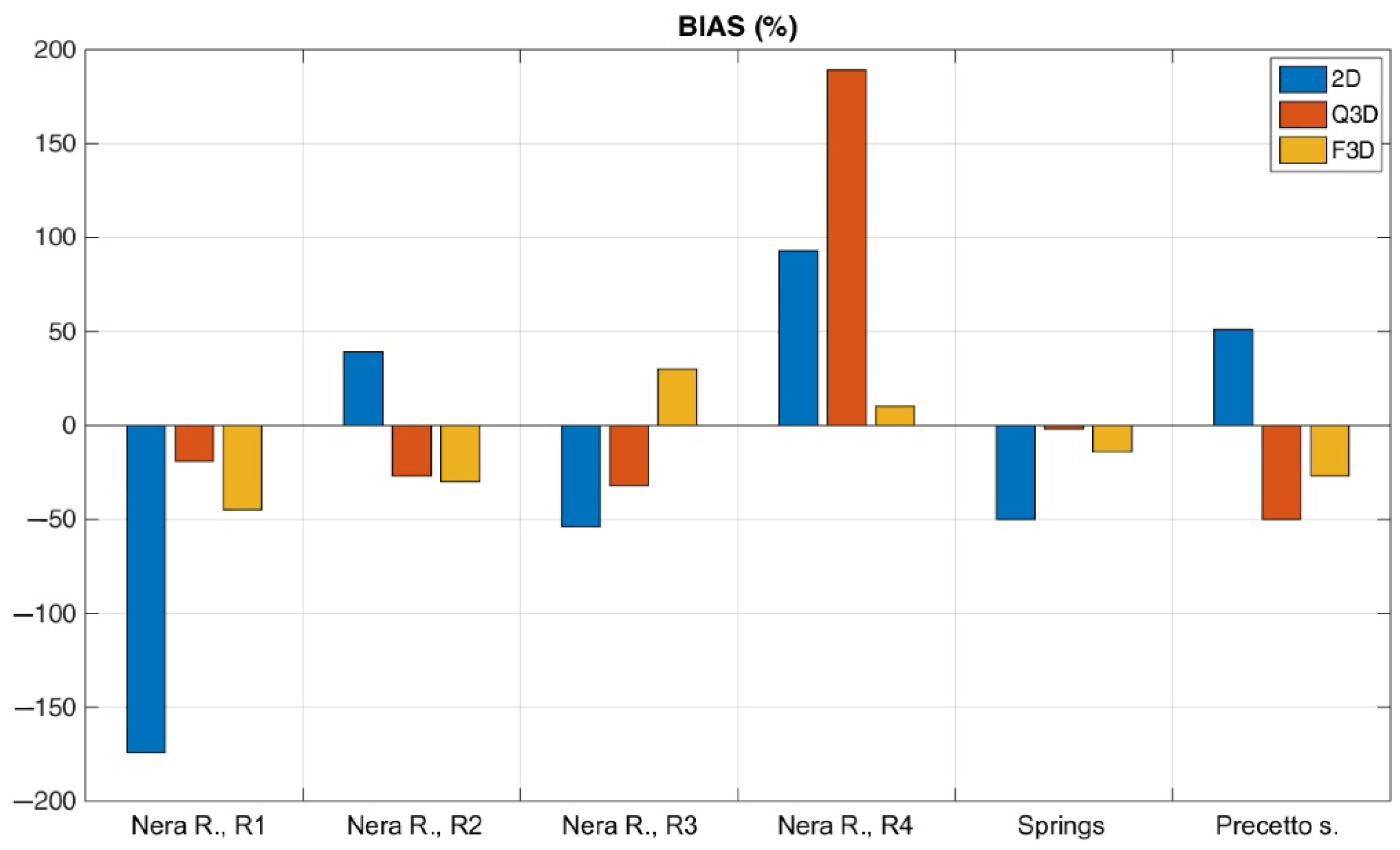
| Element | Observed | 2D | Quasi-3D | Fully 3D |
|---|---|---|---|---|
| Well Scheggino, m a.s.l. | 273 | 271.51 | 275.57 | 273.26 |
| Well Renari, m a.s.l. | 301 | 269.88 | 312.52 | 305.00 |
| Nera R., R1, l/s | 436 | −322.00 | 351.92 | 238.56 |
| Nera R., R2, l/s | 1120 | 1557.82 | 812.62 | 778.68 |
| Nera R., R3, l/s | 1110 | 507.18 | 751.17 | 1445.15 |
| Nera R., R4, l/s | 609 | 1173.95 | 1760.49 | 669.35 |
| springs, l/s | 390 | 587.99 | 195.44 | 286.21 |
| Precetto s., l/s | 120 | 60.40 | 117.71 | 103.29 |
Publisher’s Note: MDPI stays neutral with regard to jurisdictional claims in published maps and institutional affiliations. |
© 2022 by the authors. Licensee MDPI, Basel, Switzerland. This article is an open access article distributed under the terms and conditions of the Creative Commons Attribution (CC BY) license (https://creativecommons.org/licenses/by/4.0/).
Share and Cite
Preziosi, E.; Guyennon, N.; Petrangeli, A.B.; Romano, E.; Di Salvo, C. A Stepwise Modelling Approach to Identifying Structural Features That Control Groundwater Flow in a Folded Carbonate Aquifer System. Water 2022, 14, 2475. https://doi.org/10.3390/w14162475
Preziosi E, Guyennon N, Petrangeli AB, Romano E, Di Salvo C. A Stepwise Modelling Approach to Identifying Structural Features That Control Groundwater Flow in a Folded Carbonate Aquifer System. Water. 2022; 14(16):2475. https://doi.org/10.3390/w14162475
Chicago/Turabian StylePreziosi, Elisabetta, Nicolas Guyennon, Anna Bruna Petrangeli, Emanuele Romano, and Cristina Di Salvo. 2022. "A Stepwise Modelling Approach to Identifying Structural Features That Control Groundwater Flow in a Folded Carbonate Aquifer System" Water 14, no. 16: 2475. https://doi.org/10.3390/w14162475