
Determining the Flow Resistance of Racks and the Resulting Flow Dynamics in the Channel by Using the Saint-Venant Equations


Institute of Hydrosciences, Department of Civil Engineering and Environmental Sciences, Universität der Bundeswehr München, Werner-Heisenberg Weg 39, 85577 Neubiberg, Germany
*
Author to whom correspondence should be addressed.
Water 2022, 14(16), 2469; https://doi.org/10.3390/w14162469
Submission received: 28 June 2022
/
Revised: 29 July 2022
/
Accepted: 5 August 2022
/
Published: 10 August 2022
(This article belongs to the Section Hydraulics and Hydrodynamics)
Abstract
:Racks retain debris in wastewater treatment plants and shield sensitive machinery in numerous engineering applications. In open-channel flows, racks impound the upstream water level by posing local obstacles in the flow. Based on experimental investigations, empirical approaches usually predict the flow resistance by relying on Bernoulli’s energy principle. Since this principle does not correctly consider downstream conditions such as submerged flows, we present a more accurate workflow to determine the flow resistance based on the Saint-Venant equations. We will demonstrate how the loss coefficient and the hydraulic head loss are determined more reliably without adding complexity to the engineering realisation. In contrast to relying solely on two cross-sections with Bernoulli’s energy principle, applying the Saint-Venant equations enables determining the flow depth profile and the flow velocity in the entire channel. This workflow additionally allows predicting the channel’s hydraulic capacity and freeboard in arbitrary applications.
1. Introduction
Trash racks and screens have been used for decades as first process units in a wide spectrum of engineering applications. They retain suspended coarse debris and organic waste in wastewater treatment plants and shield sensitive machinery in hydropower plants, industrial plants, or pumping stations against floating or suspended trash, driftwood, and solids. Depending on the desired screening efficiency, the types are distinguished between coarse screens (clear spacing between bars , removes large debris and sediment loads), fine screens (, extracts up to small pieces), as well as micro and ultra-fine screens (, nearly filters) [1]. Their constructional design is highly diversified, including metal or wooden bar racks, wedge wires, perforated plates, mesh screens, or drum screens. Screens and racks are categorised additionally by their primary function into debris screens, security screens, weed screens, fish screens [2], or sand screens [3]. For simplicity, we conflate all these technical terms under the expression “rack” in this work.
Despite the advantages in preventing processes from clogging and aquatic species entering lethal plant sections, a rack poses (from a hydraulic point of view) a local obstacle in the flow. The installed structure causes sudden changes in the cross-section. Consequently, the flowing water is impounded upstream of the construction and is subsequently accelerated when streaming through the clear spans between the rack’s bars. However, the latter depends mainly on the downstream water level. The loss in momentum induced by the rack’s flow resistance is converted into turbulence and finally into heat. The resulting flow resistance is particularly affected by the design of the rack (bar thickness, perforation diameter, spacing, bar shape), loss-reducing features such as airfoil shapes or Coanda bars, and the flow conditions. To achieve a high degree of mechanical restrain performance with a simultaneous minimised flow resistance, rack designers are particularly concerned about the hydraulic head loss due to the flow resistance effects [4].
Determining the flow resistance of a rack is usually fostered by laboratory experiments but nowadays increasingly realised by applying computational models. The general aim is to perceive how the rack‘s flow resistance affects the overall flow dynamics in the channel. In the more recent past, several studies evaluated the influence of the rack’s properties on the head loss [5,6,7,8,9]. The recent literature rather reveals studies which yield advanced empirical equations to consider additional effects, especially the occurrence of accumulated ice and aquatic weed upstream of the rack [10,11], or to investigate angled fish-friendly bar racks [12,13,14]. Other recent studies parameterise flow effects behind the rack, such as the velocity distribution [15] and the free-surface depression [16], to yield new design equations that determine the rack head loss.
The empirical equations available in the literature have the main disadvantage that the number of empirical parameters increases, the more effects should be covered. This leads to expanded and complex mathematical expressions, which are hard to apply. Furthermore, these equations are based on Bernoulli’s energy principle, which (as we present in Section 3) is not appropriate to describe the associated flow dynamics. Moreover, the empirical equations rely mainly on the upstream flow condition but ignore downstream flow conditions. Consequently, they are prone to backwater variations.
Computational models can be used to overcome the requirement of empirical equations since the flow is usually simulated based on differential equations. Although recent studies utilised computational models to study racks [12,13,17,18,19], the workflow with 2D and 3D simulations is commonly too laborious and time-consuming to serve as a suitable design tool in everyday engineering practice.
Consequently, there is a necessity for a holistic physical approach that describes the flow dynamics in a channel with an installed rack in the best possible way with as few empirical parameters as achievable, but at the same time is highly user-friendly.
In this study, we propose a hybrid workflow by combining experimental investigations and a one-dimensional computational model to obtain the flow resistance (loss coefficient) of racks more reliably. The computational model is based on the Saint-Venant equations, which describe the flow dynamics in the main flow direction of the entire channel but can be applied very elegantly in everyday engineering practice. Using the Saint-Venant equations requires neither many empirical coefficients nor consideration of specific upstream conditions. Different backwater conditions are automatically taken into account. However, applying the Saint-Venant equations usually face the problem of how to account for local sudden losses (e.g., due to a rack) in the differential formulation. We show a way how this can be done by a transformation to a continuous loss along a certain length (e.g., rack length).
This paper is structured as follows: after we explain our experimental setup and procedure, we will present the corresponding measurement results from this study in Section 2. In Section 3, we discuss previous experimental investigations described in the literature, which determined the flow resistance of racks by using Bernoulli’s energy principle and derived empirical formulas. We will review the associated experimental workflow and evaluate the applicability to the research problem. We will show that Bernoulli’s energy principle and the empirical formulas rely on erroneous assumptions and limitations. Afterwards, we will propose a new design workflow to determine the flow resistance of racks and the resulting flow dynamics in the channel by using the Saint-Venant equations. We are going to describe the associated one-dimensional computational model in Section 4. The experimental results from Section 2 provide a comprehensive data set for model calibration. We discuss and evaluate how the proposed one-dimensional computational model (based on the Saint-Venant equations) is excellently applicable to reproduce the experimental data set by calibrating it with the sudden loss coefficient of the rack. In Section 5, we discuss the results from this study and point out the main benefit of the proposed approach. Finally, we conclude that this study proposes a contemporary state-of-the-art way to unleash the design workflow for racks from limited empirical formulas but being more accurate at the same time without featuring exorbitant complexity.
2. Materials and Methods, Experimental Investigation
2.1. Experimental Setup
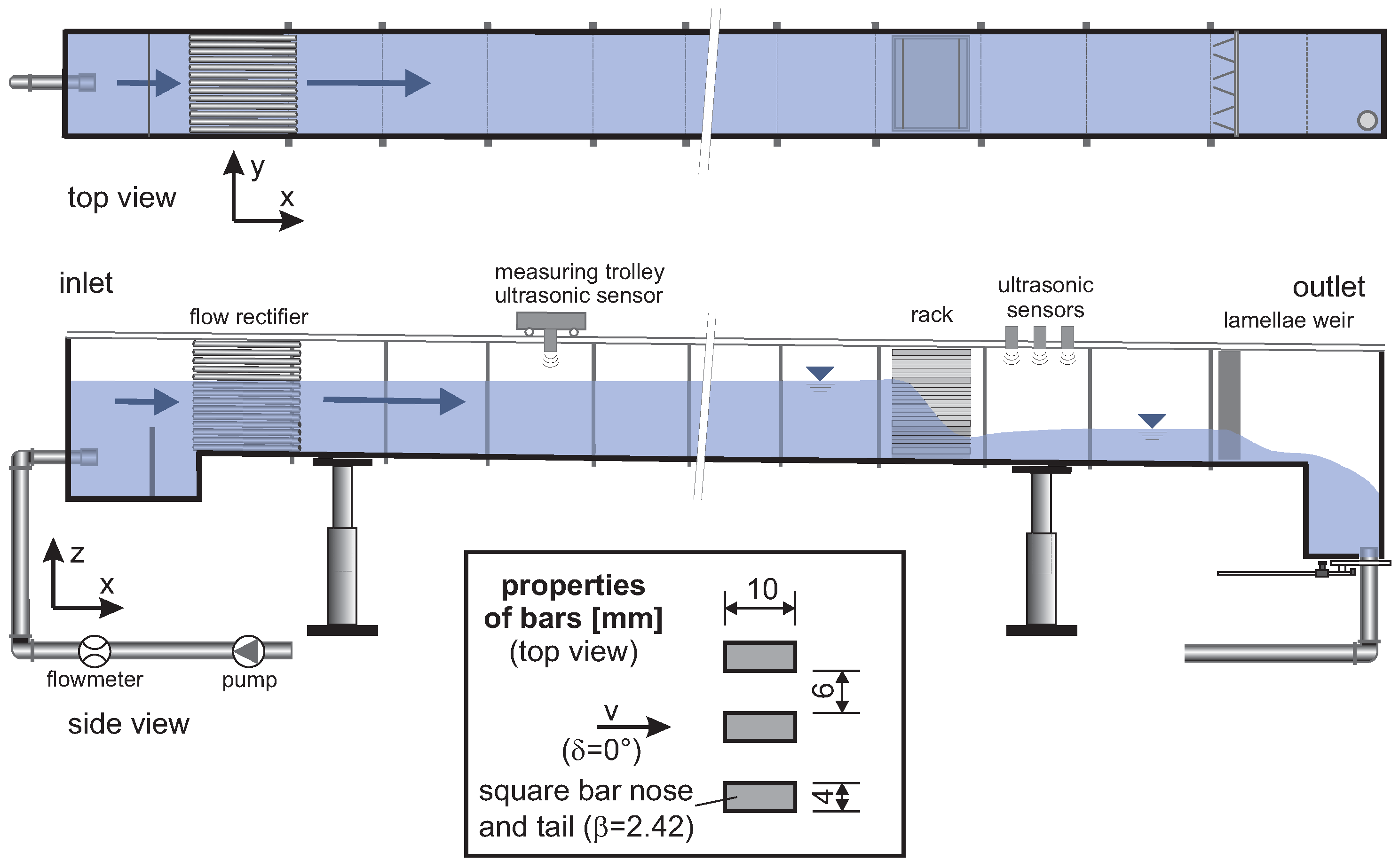
To provide reliable data sets to calibrate the Saint-Venant equations with the local resistance of the rack , several experiments were performed in a 30 m long, 0.98 m wide, and 0.97 m deep rectangular laboratory channel (Figure 1). The channel’s bottom is made of plain stainless steel, while the side walls consist of glass elements (equivalent sand roughness for both approximately ). The channel’s slope was adjusted to representing the typical flat channel slope in water treatment plants [20]. A flow rectifier at the channel’s inlet reduces turbulence and ensures a nearly one-dimensional flow (x-direction) with subordinate flow velocity components in the y- and z-directions.
We installed a 1.28 m long rack in the channel, beginning at . The rack has the following properties: clear distance between the bars , bar thickness , bar depth , bar shape coefficient (square nose and tail), blockage ratio as the ratio of the area blocked by the bars to the gross area of the trash rack . In the experiment, the inclination of the bars from the horizontal (inclination of the rack) remained at , while the angle of oblique approaching flow was consistent . Behind the rack, beginning at , rotatable vertical blades mounted in the channel served as a lamellae weir. Rotating the blades lets the channel width reduce steadily, which, in turn, induces different backwater situations. This allowed studying three flow conditions downstream of the rack:
- free outflow (unsubmerged flow): the weir provides a maximum cross-section with a net width of nearly the channel width. This condition occurs in real applications where a specific downstream flow depth is undesired or irrelevant, particularly in irrigation systems or culverts.
- medium submerged flow: the weir was closed stepwise (resulting in increasing downstream flow depth) until a downstream flow velocity between was achieved. Such velocities are usually desired in channels of water treatment plants behind the rack and before the grit chamber.
- full submerged flow: the downstream flow depth was marginally lower than the upstream one, and the difference between approach velocity and the downstream velocity was nearly negligible. This flow condition corresponds to most of the experiments described in literature.
Water with a temperature of 18 °C flowed in the channel over the laboratory pipeline system, in which an electromagnetic flowmeter gauged the discharge Q with an accuracy of 0.5% of the measured value. An ultrasonic sensor (mounted on a measuring trolley) traversed the upstream part of the rack in the longitudinal direction and determined the flow depth (Figure 1). Because the trolley could not pass the rack, three separate ultrasonic sensors measured the flow depth at fixed positions behind the rack (25.3 m, 26.0 m, 26.7 m). Each ultrasonic sensor measures the distance between the transducer and the water surface by evaluating the elapsed times between the emitted and reflected pulses with a frequency of 50 Hz. With the known distance between the transducer and the channel bottom, the water depth can be calculated. Each ultrasonic sensor has an accuracy of ±0.5 mm. Even though the flow depth downstream of the rack fluctuated in (supercritical) free outflow situations, the corresponding measured data were valid for comparison with the simulated flow depth profile. The flow velocity behind the rack decreased in submerged flow conditions (increased downstream flow depth), which damped the fluctuations noticeably and allowed a detailed comparison with the simulated data. For the three backwater conditions (free outflow, medium submerged flow, full submerged flow), we measured the flow depth in the channel for discharges between 100 and 350 in steps of 50.
2.2. Measurement Results
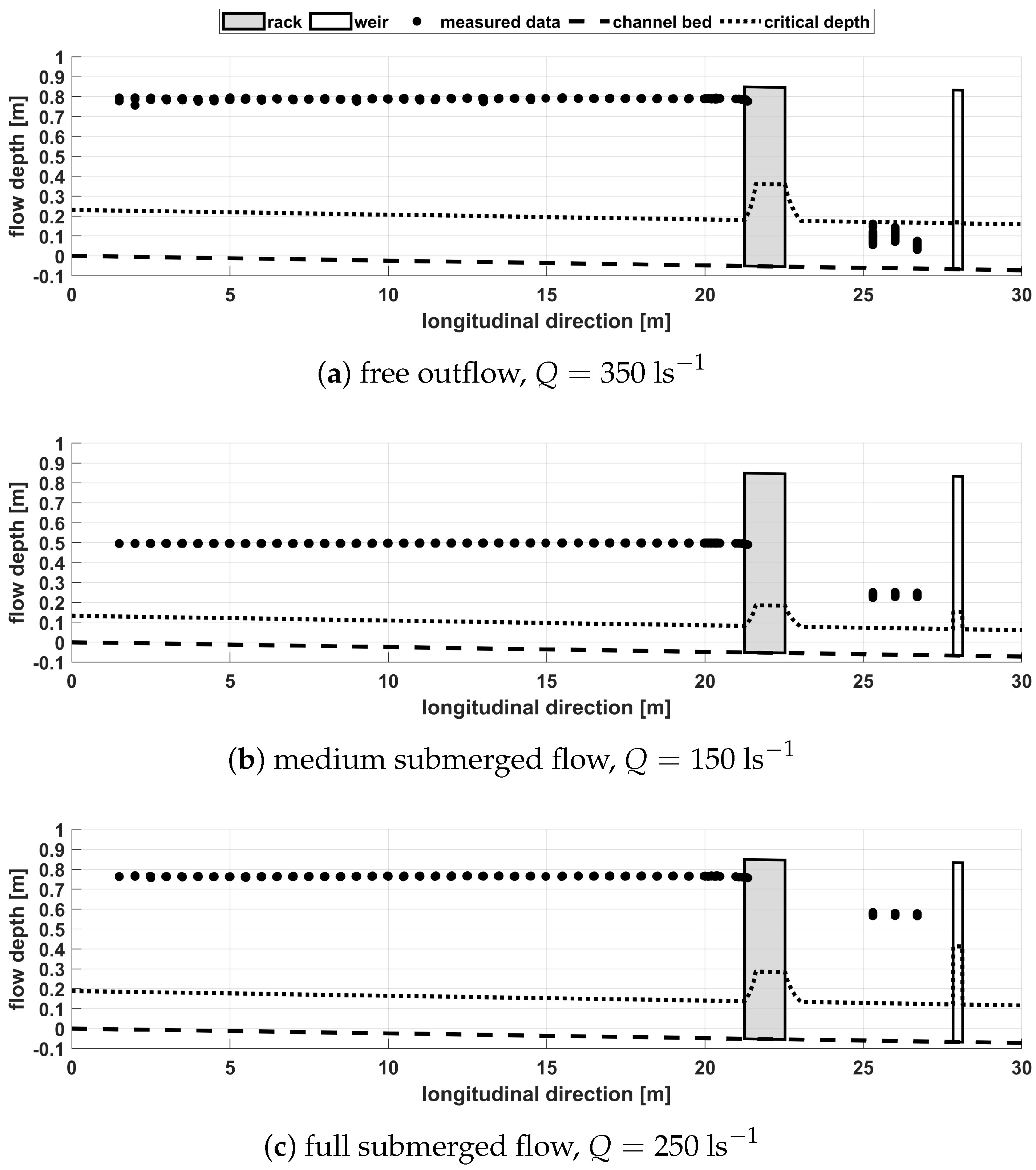
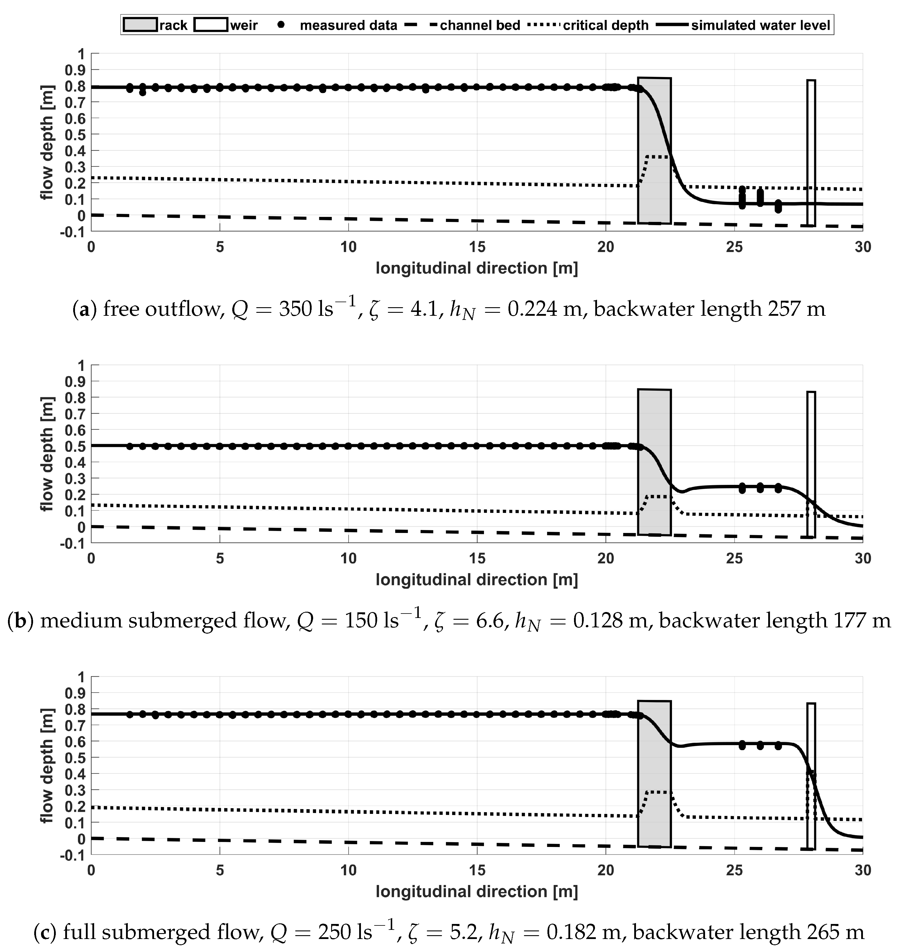
Figure 2 displays exemplary flow depth profiles for the three investigated backwater conditions. In each subfigure, a dashed line represents the channel bed, which has a negative slope due to the inclination of the channel. The black dots show the measured flow depth profile h from the laboratory experiments. In addition, the profile of the critical flow depth
is shown (dotted line), which has been calculated from the measured discharge Q, the flume’s width B, and the gravitational acceleration g. The measurement data from Figure 2 are tabulated in Appendix A. The flow is in supercritical condition if the flow depth is lower than the critical flow depth (). Subcritical conditions occur if the flow depth exceeds the critical flow depth (). For better orientation, a grey and white box marks the location of the rack and the weir, respectively.
In the experiments, the increasing flow depth in the longitudinal direction (horizontal backwater curve) indicates that the rack impounds the flow for all backwater situations. The data points directly in front of the rack show a slightly decreasing flow depth, which results from the acceleration of the flow at the rack’s intake but depends on the individual backwater condition. A lower flow depth in the downstream cross-section facilitated this effect because the inflowing water is accelerated to a greater degree, the more significant the flow depth difference is. We measured flow depths lower than the critical flow depth behind the rack (supercritical flow) for the free outflow situation. A subcritical flow occurred in both submerged flows with higher flow depths downstream of the rack (before the weir). The flow depth persists under the critical flow depth behind the weir in all cases (observed in experiments, no measured data) since the water could flow unhindered back into the laboratory reservoir at the channel’s outlet.
3. Bernoulli’s Energy Principle with Sudden Losses
For free surface flows in steady-state condition, Bernoulli’s energy equation, including continuous and sudden losses, is given as:
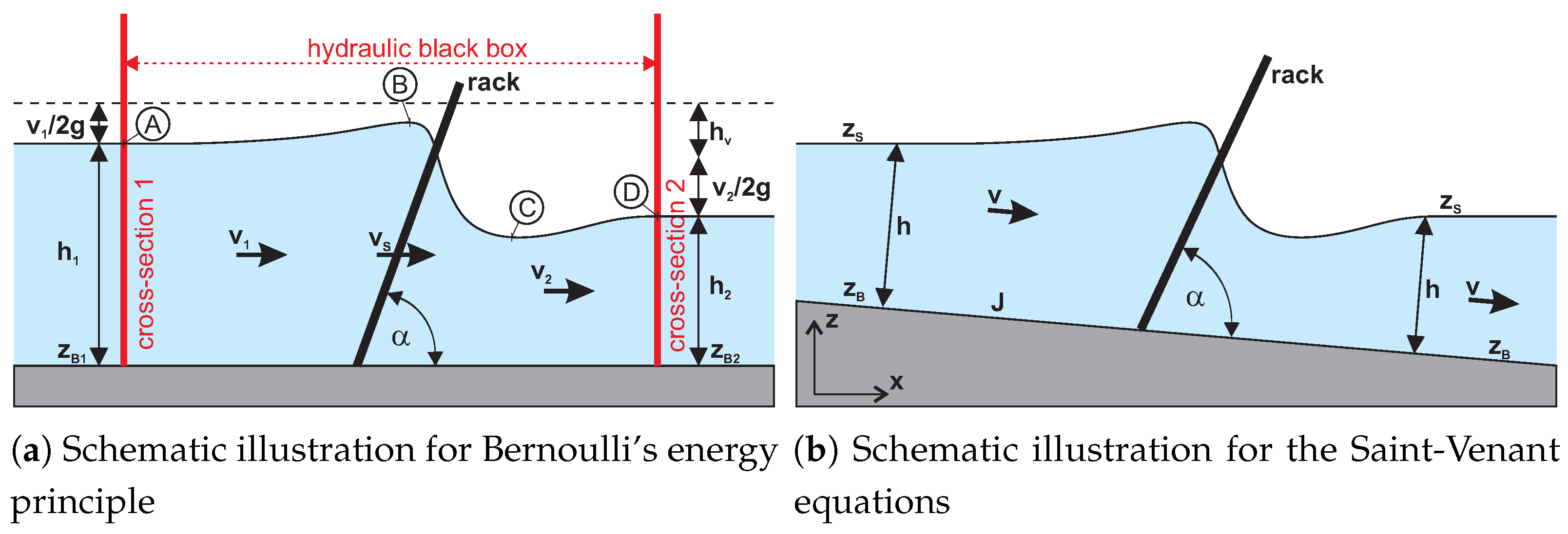
were are the bottom coordinates, the flow depths, and the average velocities. It compares the energy budget of a cross-section ahead of the rack (index 1) to another cross-section behind the rack (index 2) (Figure 3a). The fourth and fifth terms on the right side of Equation (2) describe the hydraulic head loss between both cross-sections. It contains continuous flow resistances (fourth term) due to bed, wall, and viscous friction along the investigated channel length L with the hydraulic diameter . The flow coefficient is the Weisbach friction factor [21], calculated by using the Colebrook–White formula [22]
with as the Reynolds number and as the equivalent sand roughness of the bed and wall. The fifth term of Equation (2) includes the dimensionless sudden loss coefficient describing the local resistances.
Usually, the continuous losses are neglected along the short length of a local obstacle. To study the flow resistance of racks, the sudden loss coefficient is normally related to the approach velocity ahead of the obstacle . When Bernoulli’s principle is applied directly ahead and behind the rack (Figure 3a), the bottom elevation remains constant and cancels out. Then, Equation (2) yields
In this case, also the channel width is assumed to be constant and the continuity relation is written as , with q as the specific discharge (discharge per unit width of channel). Thus, in Equation (4), the velocities can be eliminated with , which yields
3.1. Determining the Flow Resistance of a Rack
With Equation (4) or Equation (5), the sudden loss coefficient
can be directly determined from laboratory experiments after measuring the discharge and the flow depth ahead of and behind the rack. The velocities can be measured separately or are determined from the discharge, the flow depths, and the given dimensions of the channel.
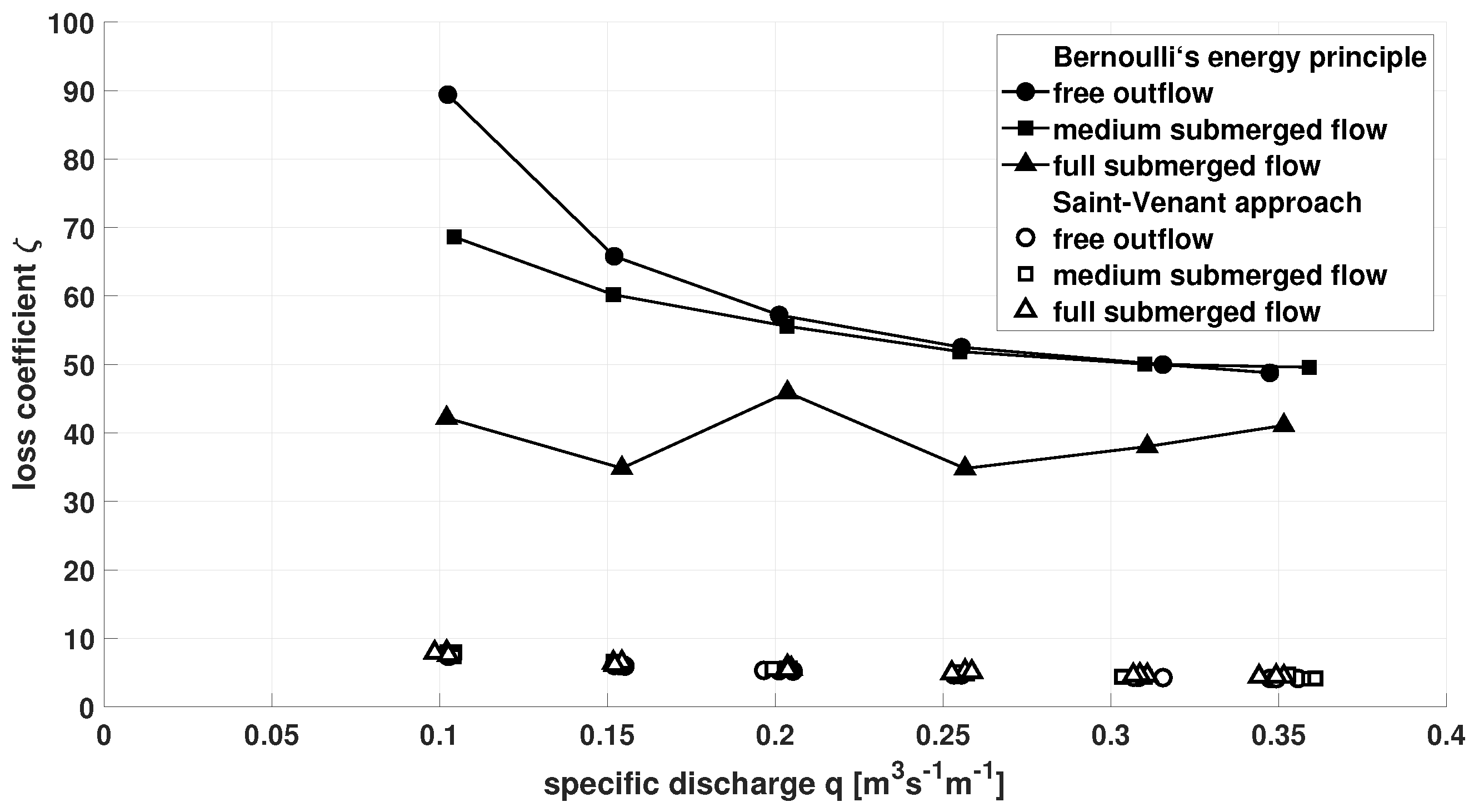
To evaluate our experiments based on Bernoulli’s energy principle, the -values were calculated by inserting the measured values of , , and q from this study into Equation (6). For , we used the median of flow depths between (directly in front of the rack). We assumed the flow depth behind the rack as the median of the measured values from the three stationary ultrasonic sensors located downstream of the rack. The discharge per unit width of the rectangular channel is known from the measured discharge Q and the channel width B. Figure 4 displays the loss coefficients as a function of the specific discharge for the three studied backwater conditions. For comparison, Figure 4 already contains the -values determined by the later-described approach with the Saint-Venant equations (Section 4). The data points reveal that Bernoulli’s energy principle leads to extremely variable values. Although the design of the rack does not alter, the loss coefficient is highly affected by the backwater situation and the flow velocity. Consequently, Bernoulli’s energy principle is not useful to adequately describe the flow resistance, at least of the rack from this study.
Although the -value characterises the rack’s individual flow resistance, Equation (6) allows no conclusion about how depends specifically on the rack’s geometrical properties. In general, the sudden loss coefficient should be a function
in particular depending on the clear distance between the bars e, the bar thickness s, a coefficient describing the shape of the bars , the inclination of the bar from the horizontal , and the angle of the approach flow . Empirical relationships for Equation (7) as a function of the geometrical dimensions has always been a research issue. A distinct -value should be determined for every specific rack design. In the best case is independent of the flow conditions. That is important to eventually predict the upstream flow depth and evaluate the available freeboard of the channel in an arbitrary scenario.
3.2. Empirical Approaches Based on Bernoulli’s Energy Principle
In most previous investigations, the flow resistance of racks was studied in detail by conducting laboratory experiments under well-controlled predefined conditions. The experimental workflow commonly consisted of installing a rack into a laboratory channel and determining the sudden loss coefficient from Equation (6) taking into account the measured discharge and the flow depths, and the given dimensions of the laboratory channel. Once was calculated, engineers set this value proportional to the given geometric and technical specifications of the rack and experimental flow conditions. Finally, empirical coefficients (e.g., the bar shape coefficient or the oblique flow coefficient) close the gap between the empirical approach and the measured data.
Reliable empirical formulas were first demanded in the first quarter of the 20th century. Because available literature was extremely sparse and partly inconsistent, the expected resistance due to racks had to be estimated by rack constructors from their professional experience. Kirschmer [23] carried out the first solid experimental investigations during his dissertation. He examined numerous variations of metal and wooden trash racks for the usage at intakes of hydropower plants. Despite considering only a straight approach of the flow, Kirschmer [23] conducted experiments with different bar thicknesses s, clear spans between the bars e, lengths and shapes of the bars, as well as trash rack angles to the horizontal . For the first time, Kirschmer [23] put the proportionalities between observed flow resistance and the physical variables on a firm foundation and correlated his experimental findings mathematically with a rack loss formula
in which is the empirically determined bar shape coefficient. In contrast to the hydraulic head loss , the flow resistance is represented solely by the flow depth difference along the rack expressing the water level differences ahead of and behind it. Kirschmer [23] already mentioned that this is not equivalent to the hydraulic head loss since it does not include the velocity differences. Although he did not consider the velocity difference (because it was small in his experiments), Kirschmer [23] took into account the (as he called it) undisturbed velocity upstream of the rack (approach velocity) in the factor of the velocity head (last factor on the right side of Equation (8)). All other parameters () form a dimensionless product that is interpreted as the sudden loss coefficient .
Since Kirschmer [23] proposed an initial mathematical formalism, several researchers improved and extended the Kirschmer formula by conducting advanced experiments or field studies. They aimed to identify the nature of for various rack conditions, in particular, regarding the influence of the discharge, clear distance between bars, bar thickness, inclination of the bar from the horizontal, angle of the approach flow, bar shape coefficient, and blockage ratio [5,8,9,24,25,26,27,28,29,30,31]. Table 1 provides a selection of empirical formulas, which are most relevant in this study. Additional formulas with similar outcomes can be found in Josiah et al. [8], Droste and Gehr [20], Spangler [25], Osborn [27], Zimmermann [28], Fellenius and Lindquist [32], Scimemi [33], Escande [34], Levin [35], United States Army Corps of Engineers [36], Sinniger and Hager [37], Hager [38], Förster and Hoff [39], Giesecke and Mosonyi [40], Uckschies [41].
Furthermore, new designs and optimisation of racks have been keeping research and development activities going. Using sophisticated measurements techniques [15,31,42,43,44,45,46] and computational fluid dynamics simulations [5,17,18,47] served to better understand the flow conditions, especially for studying partially blocked trash racks and conducting ethohydraulic investigations [12,13,14,45,46]. Some references offer specific empirical equations, tables, or graphs to determine the depth difference or hydraulic head loss depending on a vast range of rack configurations [1,36,48,49].
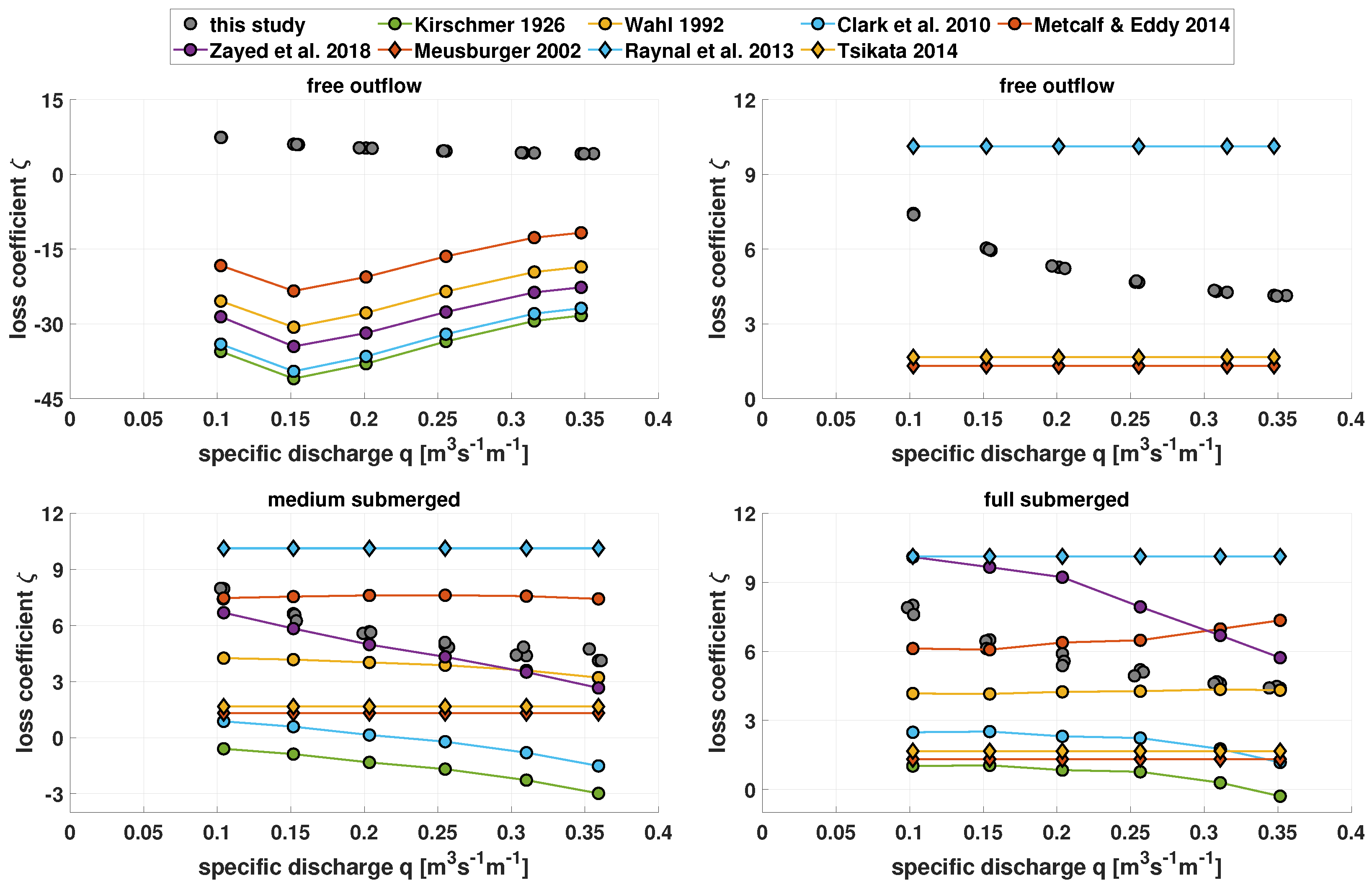
For evaluating the empirical approaches, we inserted the measured data from our experiments and the properties of the studied rack into the formulas from Table 1. The variables , , q were calculated as described in Section 3.1, while and are then known from the continuity relation. The results in Figure 5 are divided into subfigures presenting the three backwater conditions. The top left subfigure shows the results for the free outflow condition for the empirical approaches calculating the flow depth differences [1,9,23,29,50] while the top right subfigure displays the results from the equations calculating the hydraulic head loss [5,6,7]. Again, the determined -values from the later-described approach with the Saint-Venant equations (Section 4) are included in Figure 5 for comparison.

Table 1.
Selection of empirical formulas which are most relevant in this study to determine the flow depth difference or the hydraulic head loss along racks.
Table 1.
Selection of empirical formulas which are most relevant in this study to determine the flow depth difference or the hydraulic head loss along racks.
| Reference | Formula | Remarks and Particularites |
|---|---|---|
| Kirschmer [23] | flow depth difference related to approach velocity in upstream channel | |
| Wahl [29] | flow depth difference related to velocity through net flow area , regardless of bar shape and inclination angle, considers blockage ratio | |
| Meusburger [5] | considers sectional blockage of the rack, represents no sectional blockage | |
| Clark et al. [50] | investigated submerged trash racks in pressurised conduits | |
| Raynal et al. [6] | for rectangular and for hydrodynamic bars | |
| Metcalf Eddy Inc. [1] | coarse screens: fine screens: | consider an empirical discharge coefficient to account for turbulence and eddy losses: , for clean screens |
| Tsikata et al. [7] | bar shape coefficient : 3.4 for square nose and tail, 2.23 for round nose, 1.93 for streamlined bar shape | |
| Zayed et al. [9] | experiments on circular bars in subcritical flow conditions, combination of experiments and Π-theorem |
It is noticeable that, in general, none of the empirical formulas can mirror the data points from this study for the free outflow condition. The ones calculating the flow depth differences erroneously predict negative values of (Figure 5, top left subfigure), which would mean that the flow gains energy when flowing through the rack. The significant discrepancy to the data from this study (with the Saint-Venant approach) stems from suppressing the velocity difference between the upstream and downstream cross-section. We will show later, that the velocity difference cannot be neglected in the free outflow situation (Table 2). This deficiency might result from overlooking a free outflow scenario in these previous investigations. As a result, the experimentally determined coefficients calibrate the empirical approaches insufficiently to cover this particular flow condition. The empirical formulas calculating the hydraulic head loss [5,6,7] give at least positive loss coefficients (Figure 5, top right subfigure). Although the -values are mathematically independent of the flow conditions in these formulas, they cannot mirror the experimental data from this study.
The loss coefficients from the empirical formulas vary largely also for both submerged conditions (Figure 5, bottom panels). At least the results from Wahl [29] and Zayed et al. [9] are in the range of the data from this study for a medium submerged condition, so are the results from Wahl [29] and Metcalf & Eddy Inc. [1] for the full submerged condition. Overall, these findings may appear to imply that neither an energy budget between two single cross-sections (Bernoulli’s energy principle, Equation (6)) nor the available empirical formulas (Table 1) can appropriately describe the flow resistances of the rack investigated in this study. Their outcomes alter with varying backwater conditions which reveals that they do not consider the downstream flow condition appropriately.
3.3. Evaluating the Channel’s Hydraulic Capacity by Predicting the Upstream Flow Depth
Once the value of the rack’s sudden loss coefficient is determined, the upstream flow depth can be predicted when the discharge and the downstream flow depth are given, or vice versa. This measure is often necessary to predict the channel’s hydraulic capacity and freeboard affected by the rack-induced flow resistance. Using Bernoulli’s energy principle for this purpose, a third-order polynomial
can be obtained [51] by rearranging Equation (6). The ratio of the two flow depths can be expressed by
with
as the upstream Froude number [4]. The solution of this polynomial gives three roots (Figure 6a). One root is negative () and can be excluded. Therefore, two positive roots remain as a function of the upstream Froude number:
- For lower Froude numbers, the two positive roots range between . Even though both solutions are plausible (), determining one flow depth from the given other flow depth remains ambiguous.
- For a certain Froude number (depending on the value of ), these two roots unify and increase with increasing . Despite sharing the same real part, both roots have imaginary parts.
- After a particular threshold for , the roots become . That would imply that the flow depth increases after passing the rack. This solution contradicts the flow’s physics.
Consequently, the ratio of flow depths as a function of the upstream Froude number (Equation (10)) yields ambiguous and complex solutions. Bernoulli’s energy principle is, therefore, insufficient to describe the reaction of a free surface flow to sudden resistances.
For Bernoulli’s energy principle, the hydraulic head loss is commonly related to the approach velocity ahead of the rack (Equation (4)). This also affects how the sudden loss coefficient (Equation (6)) and the flow depth ratio (Equation (10)) is determined. However, using the approach velocity for the hydraulic head loss is unique in hydraulics since, except for racks, the losses are generally related to the velocity downstream of an obstacle or a perturbation. Furthermore, the upstream Froude number was used in Equation (10) to determine the flow depth ratio. However, engineers aim to predict the upstream flow depth in advance of a rack installation. Consequently, the upstream Froude number is commonly unknown in engineering practice due to the to-be-determined and . Moreover, the design workflow for trash racks and the upstream channel dimensions in water treatment plants normally starts from a channel section downstream of the rack. The flow velocities should range between behind the rack to temper the flow before entering the following grit chamber.
Applying in the hydraulic head loss term (Equation (4)) instead of and using instead of in Equation (9) to achieve Equation (10) yields again a cubic function of the flow depth ratio:
This polynomial has also three roots (Figure 6b):
- The first root is negative , revealing a non-physical process. The solution is valueless.
- The second root is greater than one: , which would imply that the flow depth increases after passing the rack. This solution also contradicts the flow’s physics.
- The third root is a purely real positive number. It is smaller or equal than one: and hence the only reasonable solution. For very small downstream velocities, such as in fully submerged conditions, the flow depth before the obstacle becomes similar to the flow depth behind it. On the contrary, the upstream flow depth will take very high values for rapid downstream flows, as in free outflow conditions.
Even though Equation (12) gives purely real solutions, practitioners now found themselves confronted with selecting the most suitable downstream Froude number (valid for a single downstream cross-section) and calculating with the discharge the downstream flow depth subsequently. Then, they must wisely choose the correct root of the polynomial to determine the flow depth ratio. Eventually, assuming is leading to a doubtful flow depth in a single predefined upstream cross-section of the rack. We like to highlight that even this alleged solution for might be fundamentally wrong since the application of Bernoulli’s energy principle is not necessarily valid for that studied flow condition.
3.4. Evaluating the Application of Bernoulli’s Energy Principle and the Empirical Formulas
Nowadays, various types of racks are in use with wide-ranging applications [2]. The available designs differ significantly concerning their physical dimensions, form and shape, or given flow conditions. The available empirical formulas were obtained from exclusive tests to determine the flow resistance of these specific rack designs causing specific validity ranges. Despite that, the achieved empirical formulas are applied to predict the hydraulic head loss (or just the flow depth difference) subsequently in real applications also for other rack designs. Despite that, the empirical formulas are applied subsequently to predict the hydraulic head loss (or just the flow depth difference) for other rack designs. Determining associated hydraulic head losses of other rack constructions by transferring empirical expressions seems unjustifiable. That is why numerous empirical design formulas for individual constructions had been developed over the years, which, in turn, had always required modified empirical coefficients.
Bernoulli’s energy principle and the empirical formulas share a long tradition in rack design, though their application stands on some erroneous assumptions and exhibits severe limitations:
Validity:
The Bernoulli energy equation is generally only valid for a steady non-rotational flow. On closer inspection, this is by no means the case when turbulent flowing water is circulating the rack’s bars and when the streams reunify afterwards because this will always induce eddies. Furthermore, Bernoulli’s energy principle compares the energy budget between two points on the same streamline. Therefore, available empirical design formulas had been derived experimentally by measurements in only two cross-sections, one ahead of and one behind the rack. The section of the rack itself remains entirely as a hydraulic black box (Figure 3a), which impedes giving evidence about the flow dynamics between the cross-sections and outside of the black box. Moreover, the empirical formulas do not mimic important hydrodynamic states in the channel, such as the longitudinal profile of the flow depth and flow velocity. They also neglect the channel slope and the continuous friction. Even if this might be reasonable for short racks, these effects can gain a noticeable influence in elongated constructions, such as (longitudinal) high angled or stepped racks.
The Undisturbed Cross-Section:
Kirschmer [23] already recognised in his experiments that the installation of a rack induces a substantial change in the water level profile. The disturbance zone, he described, comprises an impounded area in front of the rack (Ⓐ–Ⓑ in Figure 3a), a subsidence zone in the rack area (Ⓑ–Ⓒ), and an impounded area behind the rack (Ⓒ–Ⓓ). In the experiments described in the literature, this disturbance zone usually extends from about 1m in front of the rack to a few meters after the rack. According to Kirschmer [23], upstream and downstream of the disturbance zone prevails the “undisturbed” course of the water surface. Because of this, ever since Kirschmer [23], the flow variables are directly measured before Ⓐ and behind Ⓓ.
Opposed to this definition, a true undisturbed course of the water surface occurs only under normal water depth conditions. The normal depth and thus a water surface profile parallel to the channel bottom only occurs when the gravitational force of the water is equal to the friction drag along the channel, and the flow does not accelerate. Then, the normal depth can be calculated from
However, normal water depth occurs only rarely under natural conditions and can probably not be generated in laboratory channels, especially not in the 4.25 m long channel of Kirschmer [23]. Usually, man-made hydraulic structures are too short (including the 30 m long laboratory channel in this study) to let uniform flow be observed [52] and to show stretches that are uninfluenced by impoundment.
In the opinions of the authors, Kirschmer [23] and the researchers, who built upon his definition, evaluate the water surface profile in the channel qualitatively without the rack in comparison with after the rack has been installed. However, then the flow variables should be measured in an actual undisturbed cross-section upstream of the rack, where the same water level prevails as if the rack is absent: . Such a cross-section would be at the most upstream point of the backwater curve, the point in the channel up to which the water level has been artificially raised by the rack-induced impoundment. The distance between the obstacle (perturbation) and the end of the backwater curve is called the backwater length [53]. However, the end of the backwater curve will be far upstream of the rack and not within the first meters as assumed in the literature. The later-presented simulation results will confirm that the end of the backwater curve and thus the true undisturbed upstream cross-section is typically located several hundred meters in front of the rack. Although it depends on the flow conditions, the end of the backwater curve will not be detectable in rather short laboratory channels. Only when the upstream flow is in supercritical condition (which is undesired in the case of racks) the backwater length could be relatively short.
In conclusion, what Kirschmer [23] calls pointⒶdoes not mark a hydraulic undisturbed cross-section. The relatively short impounded zone in front of the rack is indeed induced by the dynamic pressure and turbulence due to the obstacle, similar to the situation at bridge piers. This leads to the conclusion that the impoundment, which is induced by the rack, is not appropriately considered in the previous measurements (particularly the upstream measurements). For an appropriate application of Bernoulli’s energy principle, the variables and must be measured upstream of the backwater curve, which seems unfeasible under laboratory conditions. Moreover, since the backwater curve would reach far upstream of the rack, the continuous losses and the channel slope could not be neglected anymore.
Measurements in the Downstream Cross-Section:
Measuring the relevant variables downstream of the rack (cross-section 2 in Figure 3a) is often associated with high uncertainties. The flow behind the rack features principally high turbulence, which could lead to a strongly fluctuating flow depth, might induce standing waves, or could provoke air bubbles in the water column. As a result, the downstream water levels are highly volatile behind the rack. Then, the question often arises where and how the desired variables should be measured in a most appropriate manner in the downstream cross-section. Or, the measurement section must be located very far downstream from the rack where the water surface is smoother, leading to an even increased disregard of channel slope and continuous friction.
Ambiguous Evaluation of the Experiments:
In the literature, the terminology head loss is sometimes erroneously mistaken for the hydraulic head loss , and their designations are often ambiguous. For this reason we name the flow depth difference, while is the hydraulic head loss.
Furthermore, some references erroneously believe that Kirschmer [23] proposed a rack loss formula describing the hydraulic head loss, but that is not true. Kirschmer [23] points out that he neglects the velocity differences and provides a flow depth difference formula. Thus, applying the Kirschmer formula for a condition with a noticeable velocity difference (free outflow scenarios) will overestimate the hydraulic head loss. Other references evaluate their experiments with the hydraulic head loss formula but call this erroneously the head loss (meaning flow depth difference). That is why the literature contains rack loss formulas describing either the flow depth difference or the hydraulic head loss (Table 1).
To overcome the erroneous assumptions and limitations of Bernoulli’s energy principle and the empirical formulas, we present a physically founded, more accurate, and more contemporary procedure to determine the loss coefficient of racks, the associated hydraulic head loss , and the resulting entire longitudinal flow depth profile in the channel. The inadequate hydraulic black box will, therefore, become superfluous.
4. Result of the Study: Applying the Saint-Venant Equations to Determine the Flow Resistance of Racks
4.1. The Saint-Venant Equations including Local Resistances
The Saint-Venant equations describe the infinitesimal mass and momentum balance in an (at least) 1D approach (Figure 3b). Hydraulic losses can generally be considered by the hydraulic head loss
including the local resistance due to the rack expressed by and continuous flow resistances along a length L by the flow coefficient (Weisbach friction factor [21], Equation (3)). However, the 1D-momentum equation cannot depict ideal sudden losses without a specific accompanying spatial extension. Consequently, the sudden loss of the rack must always be attributed to a rack’s representative length and to the associated sudden loss coefficient . Then, the momentum balance yields:
with as the vertical coordinate of the bottom surface, as the turbulent viscosity, and as the hydraulic diameter. The sudden loss coefficient must be taken into account only in that region on the longitudinal grid where the rack is positioned. Consequently, the grid resolution must be finer than the characteristic length of the rack’s sudden loss.
The momentum equation (Equation (15)) and the mass balance for the cross-section A
form the Saint-Venant equations.
4.2. Solving the Saint-Venant Equations in Matlab®
Matlab® solves parabolic (or elliptical) partial differential equation systems numerically by using the pdepde function [54]. For this, the pdepde algorithm expects the partial differential equations presented in a particular standard form
The variable x represents the independent spatial variable and t is the independent time variable, respectively. The dependent variable u is differentiated with respect to x and t, and is the partial spatial derivative. The coefficients c, f, and s represent the coefficients in the partial differential equations and are coded in terms of the input variables x, t, u, and . The constant m indicates whether the equations are written in Cartesian (, as in this study), in cylindrical (), or in spherical coordinates () [54].
In the standard form (Equation (17)), the general solution vector u can consist of several entries. For Equations (15) and (16), the solution vector consists of the cross-section A (and consequently the flow depth h) and the flow velocity v. The coefficients c, f, and s must be defined in such a way that Equations (15) and (16) are obtained. In Appendix B, we present and explain an exemplary source code to implement the 1D-Saint-Venant equations in the pdepe function for a rectangular cross-section, including the local resistance due to the rack and continuous flow resistances. Additionally, we provide a detailed executable example in the Supplementary Material.
The simulation requires the formulation of appropriate boundary conditions. Since the simulation should reflect the experimental process in this study, the measured discharge from the experiments is supplied at the inlet boundary. The measured flow depth at the farthest upstream measurement location sets the corresponding flow depth at the inlet: Dirichlet boundary condition . At the outlet, the velocity should follow a horizontal profile: Neumann boundary condition .
The numerical model still contains the to-be-determined local resistance of the rack . Thus, accurate experiments are necessary to calibrate the numerical model. In view of this, adjusting to superimpose the simulated longitudinal flow depth profile with the measured data from our well-controlled experiments will reveal the local resistance of the investigated rack from this study.
4.3. Model Calibration
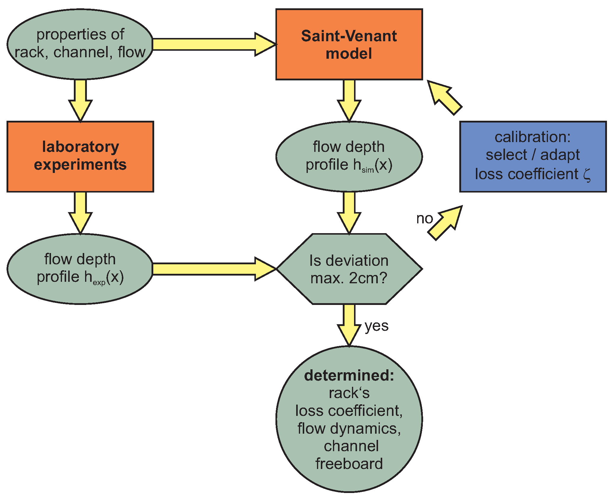
To calibrate the Saint-Venant model, the loss coefficient was adjusted iteratively in the simulation until the median of the differences between simulated flow depth and measured data fell below 2 cm. We have chosen this threshold because the value of 2 cm corresponds with the measured flow depth fluctuations and the amplitude of standings waves at the channel’s inlet. The flowchart in Figure 7 illustrates the principal hybrid workflow to determine the loss coefficient of the rack, the entire flow dynamics, and the channel freeboard. Figure 8 displays the simulated flow depth profiles as continuous lines, revealing excellent agreement with the measured data upstream of the rack. Even though the measured data fluctuate slightly behind the rack in the free outflow condition, the flow depth is covered satisfactorily by the simulated flow depth profile. For both submerged conditions, the simulated flow depth profiles match the downstream data points very accurately, although only the net width of the weir governs the downstream flow depth in the simulations.
We summarise our data in Table 2. The -values determined with the Saint-Venant approach were already displayed in advance in Figure 4 and Figure 5 for comparison with the results from Bernoulli’s energy principle and the empirical approaches. The -values from this study range between and decrease with increasing discharge (Table 2). The sudden loss coefficient in this study depends slightly on the flow condition because the contraction of the cross-section at the rack’s intake influences the flow dynamics. The resulting overall flow resistance of the rack is, therefore, slightly affected by the flow velocity. Importantly, the -values are nearly independent of the backwater conditions. On one hand, this seems reasonable since the loss coefficient describes the characteristics of the rack construction and should generally be independent of the downstream flow conditions. However, on the other hand, this cannot necessarily be generalised and might be the case for this explicit rack construction only.
Overall, the channel bottom and the glass walls have a plain surface in our setup. Consequently, the flow resistance of the rack (expressed by ) exceeded the resistance due to the surface roughness along the 30 m long channel (expressed by ) by a factor of at least 10.
To compare the magnitude of the flow depth difference (Table 2, third column) with the velocity head difference (Table 2, fourth column), we used again our experimentally determined flow depths and (evaluated as described in Section 3.1). The corresponding velocities were calculated with the specific discharge q. The data in Table 2 reveals that the velocity head difference gains considerable influence in medium submerged (values in the order of centimetres) and free outflow conditions (velocity head differences about 30% of the flow depth difference), and can therefore not be ignored. In contrast, the influence of the velocity head differences can justifiably be neglected in full submerged flows since the values range only on the order of millimetres.
5. Discussion
Engineers and practitioners utilise screens and racks in numerous hydraulic applications. However, each construction will induce a hydraulic head loss in the flow that impounds the incoming water in front of the rack. The flow condition behind the rack, in turn, depends on the kind of application and can vary noticeably. Investigating the hydraulic head loss in experiments and determining the rack‘s flow resistance as precisely as possible has motivated researchers and practitioners for years. Available empirical formulas in literature (mainly describing the flow depth difference instead of the hydraulic head loss) solely compare the energy budget between two cross-sections in the channel.
Numerous literature references present empirical formulas for estimating the flow resistance induced by a rack. Although some of them consider many effects and, thus, provide a comprehensive design formalism [5,9,55], they always originate from comparing the experimentally-determined energy head in two cross-sections, ahead of and behind the rack (applying Bernoulli’s energy principle). The flow depth difference or the hydraulic head loss between the cross-sections is put subsequently in relation to the physical dimensions of the rack. Afterwards, the inconsistency between the empirical approach and measured values is projected to the magnitude of particular empirical coefficients (e.g., bar shape or effect of oblique inflow) or compensated by additional (physically unidentified) coefficients. When this black box hydraulics method is applied, it solely considers the flow conditions in two cross-sections but neglects important variables such as channel slope or bottom friction. The corresponding results are thus highly susceptible. A modified channel geometry or altered flow situation will consistently question the achieved state of the art or require a readjustment of the obtained coefficients.
Moreover, the latest considerations of specific effects upstream of the rack [8,10,11,16,50] are generally valuable in engineering practice. However, they add extra empirical coefficients to the existing design equations to determine the rack head loss. This expands the overall mathematical expressions and leads to complex formalism without increasing the reliability, in particular, because different backwater situations are not considered.
We proposed a more contemporary and continuous approach. Our workflow relies on the Saint-Venant equations, which we implemented in a one-dimensional computational model to simulate the flow depth and the flow velocity in the entire channel, including the rack and a downstream weir. Despite the rack’s loss coefficient , the hybrid approach does not require other empirical coefficients or predefined upstream flow conditions and takes different backwater conditions automatically into account. We solved the problem of how to account for the local sudden loss due to the rack in the differential formulation by transforming it into a continuous loss along the rack length.
The model performed excellently in reproducing the obtained experimental data from this study by maintaining a maximum deviation of the simulated flow depth profile from the experimental data of only 2 cm (predefined threshold as explained in Section 4.3). The calibration process resulted in a set of dimensionless loss coefficients (representing the rack’s flow resistance) for varying discharges and backwater conditions. In contrast to Bernoulli’s energy principle (Figure 4) and to the majority of the empirical formulas (Figure 5), the proposed approach does not show a significant dependency on the backwater flow conditions and is, moreover, not limited to certain rack types, particular properties (type of perforation, bar shape, constructional material), or field of application. Moreover, the Saint-Venant equations take into account channel slope and bottom friction.
The procedure from this study relies on a one-dimensional model describing the flow dynamics in the longitudinal direction of the channel. However, this limitation does not affect the potential application considerably. In most hydraulic applications, technical channels have a distinctly defined structure (rectangular or trapezoidal cross-section) and a straight-line course. Examining the flow in a one-dimensional model might be a reasonable approximation.
Admittedly, the flow in the channel section, where the rack is installed, can be studied in more detail with 2D or 3D computational models [5,12,17,18,47]. By automatically considering lateral and vertical flow components, seminal insights into the turbulent flow around the bars or ethohydraulic effects [12,13] can be elaborated. This can eventually promote further development of rack designs or initiates advanced scientific investigations. However, since such simulations are still relatively computationally intensive and time-consuming, the outcomes (in fine grid resolution) are usually constrained to a limited channel section. Furthermore, 2D or 3D computational models are generally not easily practicable in engineering practice to determine the flow dynamics in the entire channel. The effort to apply them is usually too high to visualise quasi one-dimensional flows, such as in water treatment plants or irrigation systems.
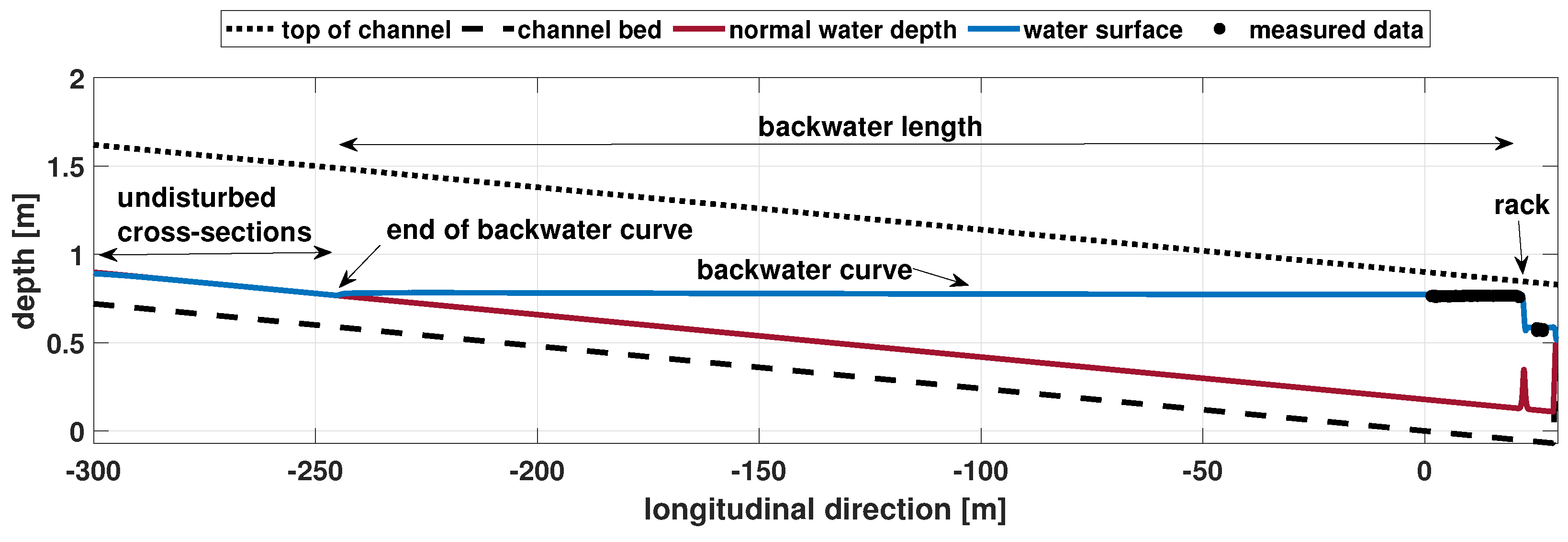
The main benefit of our proposed approach lies in comprehensively describing the flow dynamics in the channel but being applicable in everyday engineering practice. The flow depth profile and the flow velocity are not restricted to single cross-sections but are continuously obtainable along the channel (only limited by the grid size in the simulations). For example, for Figure 9, the simulation area from Figure 2c was extended in the upstream direction to simulate the flow dynamics in a 330 m long channel. The water surface profile and the normal water depth reveal that the impoundment due to the rack reaches very far upstream. The Saint-Venant equations output automatically the complete backwater curve and pinpoint the upstream undisturbed cross-section. The latter is located 265 m upstream of the rack (x = −243.7 m), which confirms that a true undisturbed cross-section could not be reached in a laboratory channel.
With detailed knowledge of the rack‘s flow resistance, the upstream flow depth can be predicted. As we showed in Section 3.3, the flow depth ratio and the upstream flow depth can be arbitrarily determined when using Bernoulli’s energy principle. Applying the Saint-Venant equations as proposed in this work renders all the problems and deficiencies mentioned in Section 3.3 obsolete. Once the rack’s local resistance has been determined by reproducing the experimental findings, the entire longitudinal flow depth profile in the channel, including the depth-averaged velocities, can be predicted elegantly by solving the Saint-Venant equations for a particular engineering application. For this purpose, the channel properties, the discharge, and the desired downstream flow depth must only be set in the Saint-Venant model. Thus, in contrast to Equations (10) and (12), applying the Saint-Venant equations gives one unique and distinct solution for the upstream flow depth.
Besides the flow resistance of an installed rack, the Saint-Venant equations can simultaneously consider additional flow effects on the longitudinal grid, such as local variations in the channel’s geometry, the channel slope, or the basal roughness. The empirical approaches cannot take these effects into account. Furthermore, the Saint-Venant equations allow to investigate the resistances of individual rack components or attachment parts along the channel by adding additional values on the grid. The Saint-Venant equations allow connecting coarse and fine screens in series comfortably, as individual loss coefficients result in each case. In contrast, the empirical approaches must assess the flow resistance of each rack separately without considering mutual flow interaction. Moreover, local variations of the channel geometry, such as sudden or continuous contractions, or steps in front of the rack, can be considered in the simulation. When applying the empirical approaches, the effects from these segments would be mistakenly assigned either to the rack’s loss coefficient or to specific empirical parameters (e.g., the bar shape coefficient).
In this study, we investigated a single rack construction and provide the -values under varying discharges and backwater conditions only for this construction. Previous benchmark experiments [5,6,7,9,50,55] have conducted much more comprehensive investigations by varying different rack properties (e.g., the clear distance between the bars, the bar thickness, the inclination of the bar from the horizontal, angle of the approach flow, and bar shape). However, we did not aim to determine numerous -values for various rack configurations but intended to point out a new workflow on an exemplary rack.
For an application of the Saint-Venant model in everyday engineering practice (e.g., to determine the hydraulic capacity and freeboard of a channel), reliable -values are essential but not available yet from an approach as proposed in this study. Nonetheless, there are two options to achieve a comprehensive data set of -values.
- Option 1: The experiments from the literature will be repeated, but this time by measuring the longitudinal flow depth profile in the channel instead of the flow depth in just two cross-sections. Then, following our workflow, the -values are determined by calibrating the Saint-Venant model with the measurement results. Although option 1 will give a reliable and comprehensive data set, realising this requires diligence due to numerous necessary experiments and possible combinations of rack parameters.
- Option 2: The experimental conditions (setup, flow properties, rack characteristics) are generally well-described in the corresponding literature. The measured flow depths are usually documented in (at least) two cross-sections (in front of and behind the rack). The Saint-Venant model can be applied to reproduce the flow dynamics in the channel by identifying the most appropriate -value such that the simulated flow depth profile superimposes best with the (at least) two available flow depth values. Finding the -values with this option is more convenient than option 1 but offers a higher uncertainty due to less empirical data. However, the effect of altering the clear distance between the bars or the bar thickness can be directly studied in the Saint-Venant model since e and s form the blockage ratio p, which determines the net width of the rack.
6. Conclusions
With this study, we put the determination of the rack’s resistance on a sound physical base. Our contemporary approach uses the Saint-Venant equations that describe the flow dynamics in the entire channel by relying exclusively on the rack’s loss coefficient. We calibrated our approach (up to a calibration efficiency for the flow depth: 2 cm) based on well-controlled laboratory experiments. We have considered different discharges as well as three backwater situations (free outflow, medium submerged, full submerged). Our results indicate that the obtained rack’s flow resistances do not vary significantly for the different flow conditions. This shows the maturity of the hybrid approach.
The engineering practice demands an appropriate and practical workflow to determine the flow resistance of a rack and the resulting upstream impoundment. Our approach must also fulfil this requirement.
For a certain channel and rack, the proposed workflow consists of the following three steps:
- As a first step, well-documented experiments under controlled conditions should provide detailed flow depth profiles under varying discharges and backwater situations. For similar flow conditions, rack and channel properties, literature data from previous experiments can also be used as a substitute (above-mentioned option 2).
- Afterwards, the Saint-Venant model is calibrated to the measured data by determining the rack’s loss coefficient . The provided executable example in the Supplementary Materials can be adapted for that purpose.
- Then, the Saint-Venant equations can simulate the flow depth profile (and the velocity) for an arbitrary application considering an installed rack. As a result, the respective flow velocities and the freeboard are available at any point in the channel.
The simulation has the additional advantage that the hydraulic capacity of a designed channel can be predicted already in the planning phase of new constructions, enabling the engineers to derive the optimal cross-section geometry. This procedure is particularly valuable for standardised rack constructions or modules. Manufacturers must only once determine the specific -value of the rack and can subsequently implement it into the Saint-Venant model to utilise the simulation as a design tool. The effort required for generating a water surface profile like in Figure 8 is indeed very moderate since solving the Saint-Venant equation took about 5 min on a commercial computer in this study.
The benefit of the approach proposed in this study can be enhanced if the previous experiments in the literature are repeated and evaluated with the Saint-Venant model. Although requiring diligence, this will eventually lead to a large set of -values, from which advanced relationships for rack properties can be extracted. We point out a proper way for a hybrid workflow with the (above-mentioned) options 1 and 2.
Finally, we used the Matlab® environment for conducting this study. Hence, the executable example provided in the Supplementary Materials performs best for Matlab® applications. Nevertheless, implementing the Saint-Venant model into other computing platforms is also feasible. Since, besides Matlab®, Octave, PythonTM, Maple, and Mathematica are widespread in engineering practice, the proposed approach from this study might contribute to determining the flow resistance of racks and the resulting flow dynamics more reliable and in a more contemporary way without adding complexity to the engineering application.
Supplementary Materials
The following supporting information can be downloaded at: https://www.mdpi.com/article/10.3390/w14162469/s1, SVM1D_main.m is the main file and contains all the necessary information to run the executable example.
Author Contributions
Conceptualization, I.B. and A.M.; methodology, I.B. and A.M.; software, I.B. and A.M.; validation, I.B.; formal analysis, I.B. and A.M.; investigation, I.B.; resources, I.B. and A.M.; data curation, I.B.; writing—original draft preparation, I.B.; writing—review and editing, I.B. and A.M.; visualization, I.B.; supervision, A.M.; project administration, I.B. and A.M.; funding acquisition, I.B. All authors have read and agreed to the published version of the manuscript.
Funding
We acknowledge financial support by Universität der Bundeswehr München.
Institutional Review Board Statement
Not applicable.
Informed Consent Statement
Not applicable.
Data Availability Statement
An executable example of the Matlab® source code of the Saint-Venant model is available in the Supplementary Material.
Acknowledgments
The authors would like to thank the laboratory staff of the Institute of Hydroscience for their technical support during the project.
Conflicts of Interest
The authors declare no conflict to interest.
Notation
The following symbols are used in this paper:
| d | bar depth [m] |
| hydraulic diameter [m] | |
| e | clear distance between the bars [m] |
| gravitational acceleration [] | |
| h | flow depth [m] |
| upstream flow depth (in front of the rack) [m] | |
| downstream flow depth (behind the rack) [m] | |
| critical flow depth [m] | |
| normal water depth [m] | |
| hydraulic head loss [m] | |
| flow depth difference [m] | |
| equivalent sand roughness [m] | |
| blockage ratio [1] | |
| specific discharge [] | |
| s | bar thickness [m] |
| t | time [s] |
| approach (upstream) velocity [] | |
| downstream velocity [] | |
| flow velocity through the openings of the rack [] | |
| x | longitudinal coordinate [m] |
| y | lateral coordinate [m] |
| z | vertical coordinate [m] |
| bottom coordinates [m] | |
| A | area of cross-section [] |
| B | channel width [m] |
| Froude number [1] | |
| J | channel slope [1] |
| L | length [m] |
| length of sudden loss [m] | |
| Q | discharge [] |
| Reynolds number [1] | |
| inclination of the bar from the horizontal [] | |
| bar shape coefficient [1] | |
| angle of the approach flow [] | |
| sudden loss coefficient [1] | |
| Weisbach friction coefficient [1] |
Appendix A. Experimental Data
Table A1.
Data for flow depth and critical flow depth for the three results from Figure 2.
Table A1.
Data for flow depth and critical flow depth for the three results from Figure 2.
| Long. Direction | Free Outflow | Medium Submerged | Full Submerged | |||
|---|---|---|---|---|---|---|
| x[m] | h[m] | [m] | h[m] | [m] | [m] | [m] |
| 2.47 | 0.793 | 0.231 | 0.502 | 0.133 | 0.772 | 0.189 |
| 2.97 | 0.796 | 0.231 | 0.503 | 0.133 | 0.771 | 0.189 |
| 3.47 | 0.796 | 0.231 | 0.504 | 0.133 | 0.772 | 0.189 |
| 3.97 | 0.795 | 0.231 | 0.505 | 0.133 | 0.773 | 0.189 |
| 4.47 | 0.798 | 0.231 | 0.507 | 0.133 | 0.773 | 0.189 |
| 4.97 | 0.798 | 0.231 | 0.508 | 0.133 | 0.775 | 0.189 |
| 5.47 | 0.799 | 0.231 | 0.508 | 0.133 | 0.774 | 0.189 |
| 5.97 | 0.802 | 0.231 | 0.510 | 0.133 | 0.777 | 0.189 |
| 6.47 | 0.806 | 0.231 | 0.511 | 0.133 | 0.778 | 0.189 |
| 6.97 | 0.805 | 0.231 | 0.512 | 0.133 | 0.780 | 0.189 |
| 7.47 | 0.804 | 0.231 | 0.514 | 0.133 | 0.781 | 0.189 |
| 7.97 | 0.806 | 0.231 | 0.515 | 0.133 | 0.783 | 0.189 |
| 8.47 | 0.807 | 0.231 | 0.516 | 0.133 | 0.783 | 0.189 |
| 8.97 | 0.808 | 0.231 | 0.517 | 0.133 | 0.786 | 0.189 |
| 9.47 | 0.811 | 0.231 | 0.518 | 0.133 | 0.787 | 0.189 |
| 9.97 | 0.813 | 0.231 | 0.521 | 0.133 | 0.791 | 0.189 |
| 10.47 | 0.814 | 0.231 | 0.523 | 0.133 | 0.787 | 0.189 |
| 10.97 | 0.815 | 0.231 | 0.523 | 0.133 | 0.792 | 0.189 |
| 11.47 | 0.809 | 0.231 | 0.525 | 0.133 | 0.791 | 0.189 |
| 11.97 | 0.821 | 0.231 | 0.526 | 0.133 | 0.792 | 0.189 |
| 12.47 | 0.821 | 0.231 | 0.528 | 0.133 | 0.796 | 0.189 |
| 12.97 | 0.822 | 0.231 | 0.529 | 0.133 | 0.797 | 0.189 |
| 13.47 | 0.820 | 0.231 | 0.531 | 0.133 | 0.798 | 0.189 |
| 13.97 | 0.824 | 0.231 | 0.531 | 0.133 | 0.798 | 0.189 |
| 14.47 | 0.824 | 0.231 | 0.533 | 0.133 | 0.800 | 0.189 |
| 14.97 | 0.827 | 0.231 | 0.534 | 0.133 | 0.800 | 0.189 |
| 15.47 | 0.828 | 0.231 | 0.535 | 0.133 | 0.801 | 0.189 |
| 15.47 | 0.826 | 0.231 | 0.536 | 0.133 | 0.801 | 0.189 |
| 16.47 | 0.830 | 0.231 | 0.538 | 0.133 | 0.804 | 0.189 |
| 16.97 | 0.830 | 0.231 | 0.539 | 0.133 | 0.806 | 0.189 |
| 17.47 | 0.831 | 0.231 | 0.540 | 0.133 | 0.807 | 0.189 |
| 17.97 | 0.833 | 0.231 | 0.541 | 0.133 | 0.808 | 0.189 |
| 18.47 | 0.833 | 0.231 | 0.542 | 0.133 | 0.809 | 0.189 |
| 18.97 | 0.834 | 0.231 | 0.543 | 0.133 | 0.811 | 0.189 |
| 19.47 | 0.835 | 0.231 | 0.544 | 0.133 | 0.811 | 0.189 |
| 19.97 | 0.836 | 0.231 | 0.545 | 0.133 | 0.814 | 0.189 |
| 20.47 | 0.840 | 0.231 | 0.547 | 0.133 | 0.813 | 0.189 |
| 20.97 | 0.839 | 0.231 | 0.547 | 0.133 | 0.814 | 0.189 |
| 21.07 | 0.839 | 0.231 | 0.547 | 0.133 | 0.812 | 0.189 |
| 21.17 | 0.835 | 0.231 | 0.546 | 0.133 | 0.812 | 0.189 |
| 21.27 | 0.830 | 0.236 | 0.544 | 0.136 | 0.809 | 0.193 |
| 21.28 | 0.832 | 0.239 | 0.543 | 0.138 | 0.810 | 0.195 |
| 21.29 | 0.829 | 0.242 | 0.543 | 0.139 | 0.809 | 0.197 |
| 21.30 | 0.835 | 0.245 | 0.543 | 0.141 | 0.809 | 0.200 |
| 21.31 | 0.829 | 0.248 | 0.543 | 0.143 | 0.809 | 0.202 |
| 21.32 | 0.830 | 0.251 | 0.542 | 0.144 | 0.809 | 0.205 |
| 21.33 | 0.828 | 0.254 | 0.542 | 0.146 | 0.807 | 0.207 |
| 21.34 | 0.827 | 0.257 | 0.542 | 0.148 | 0.807 | 0.210 |
| 21.35 | 0.827 | 0.261 | 0.541 | 0.150 | 0.808 | 0.213 |
| 26.00 | 0.175 | 0.231 | 0.301 | 0.133 | 0.635 | 0.189 |
| 25.30 | 0.156 | 0.231 | 0.300 | 0.133 | 0.636 | 0.189 |
| 26.70 | 0.118 | 0.231 | 0.301 | 0.133 | 0.636 | 0.189 |
Appendix B. Matlab® Source Code
The following source code explains one possibility to implement the 1D-Saint-Venant equations in the pdepe function for a rectangular cross-section, including the local resistance due to the rack and continuous flow resistances. For this study, we used the Matlab® version R2020b Update 1 (9.9.0.1495850).
In the standard form (Equation (17)), the general solution vector u can consist of several entries. For Equations (15) and (16), the solution vector consists of the cross-section A (and consequently the flow depth h) (source code line 2) and the flow velocity v (source code line 3). The coefficients c, f, and s must be defined in such a way that Equations (15) and (16) are obtained (source code line 8–16). Line 4 calculates the flow depth from the determined rectangular cross-section, while lines 5, 6, and 7 calculate the turbulent viscosity, hydraulic diameter, and the Weisbach friction factor.
1 function [c,f,s] = stvenant(x,t,u,DuDx) % function signature
2 A = u(1); % cross-section A as first solution of the partial diff. equ.
3 v = u(2); % velocity v as second solution of the partial diff. equ.
4 h = A/B; % calculating flow depth from cross-section and width
5 nut = abs(6*0.41/log(12*h/ks)*v*h); % approach for turbulent viscosity
6 dhyd=4*A/(B + 2*h); % hydraulic diameter
7 lambda=colebrook_white(v*dhyd/1.e-6,ks/dhyd); % Weisbach friction
8 % c,f,s are elements in Matlab standard form for pdepe
9 c = [1;1];
10 f = [-v*A;nut*DuDx(2)-v^2/2-g*h-g*zbpp(x)];
11 s = [0;-lambda/dhyd*v*abs(v)/2];
12 zeta = 5.2; % sudden loss coefficient, local resistance of the rack
13 x1 = 21.25; x2 = 21.25 + 1.28; % start and end of the rack on the grid
14 if x >= x1 && x <= x2 % consider rack only between x1 and x2
15 s = [0;-lambda/dhyd*v*abs(v)/2-zeta/(x2-x1)*v*abs(v)/2];
16 end
17 end
References
- Metcalf & Eddy Inc. Wastewater Engineering: Treatment and Resource Recovery, 5th ed.; McGraw-Hill Education: New York, NY, USA, 2014. [Google Scholar]
- Benn, J.; Kitchen, A.; Kirby, A.; Fosbeary, C.; Faulkner, D.; Latham, D.; Hemsworth, M. Culvert, Screen and Outfall Manual: CIRIA C786. 2019. Available online: https://www.ciria.org/CIRIA/News/CIRIA_news2/Culvert_screen_and_outfall_manual_C786_PR.aspx (accessed on 1 June 2022).
- James, C.S. Hydraulic Structures; Springer International Publishing: Cham, Switzerland, 2020. [Google Scholar] [CrossRef]
- Chow, V.T. Open-Channel Hydraulics; Blackburn Press: Caldwell, NJ, USA, 2009. [Google Scholar]
- Meusburger, H. Energieverluste an Einlaufrechen von Flusskraftwerken; Mtteilungen der Versuchsanstalt für Wasserbau, Hydrologie und Glaziologie Nr. 179; Eidgenössische Technische Hochschule: Zürich, Switzerland, 2002. [Google Scholar]
- Raynal, S.; Chatellier, L.; Courret, D.; Larinier, M.; David, L. An experimental study on fish-friendly trashracks—Part 2. Angled trashracks. J. Hydraul. Res. 2013, 51, 67–75. [Google Scholar] [CrossRef]
- Tsikata, J.M.; Tachie, M.F.; Katopodis, C. Open-channel turbulent flow through bar racks. J. Hydraul. Res. 2014, 52, 630–643. [Google Scholar] [CrossRef]
- Josiah, N.R.; Tissera, H.P.S.; Pathirana, K.P.P. An Experimental Investigation of Head loss through Trash Racks in Conveyance Systems. Eng. J. Inst. Eng. 2016, 49, 1. [Google Scholar] [CrossRef]
- Zayed, M.; El Molla, A.; Sallah, M. An experimental study on angled trash screen in open channels. Alex. Eng. J. 2018, 57, 3067–3074. [Google Scholar] [CrossRef]
- Salah Abd Elmoaty, M. An experimental investigation of the impact of aquatic weeds trash racks on water surface profile in open channels. Water Sci. 2019, 33, 84–92. [Google Scholar] [CrossRef] [Green Version]
- Walczak, N.; Walczak, Z.; Nieć, J. Assessment of the Resistance Value of Trash Racks at a Small Hydropower Plant Operating at Low Temperature. Energies 2020, 13, 1775. [Google Scholar] [CrossRef] [Green Version]
- Gisen, D. Modeling Upstream Fish Migration in Small-Scale Using the Eulerian-Lagrangian-Agent Method (ELAM): BAW Dissertationen Nr. 1. Ph.D. Thesis, Universität der Bundeswehr München, Neubiberg, Germany, 2018. [Google Scholar]
- Beck, C. Fish Protection and Fish Guidance at Water Intakes Using Innovative Curved-Bar Rack bypass Systems: VAW Mitteilungen Nr. 257. Ph.D. Thesis, ETH Zurich, Zurich, Switzerland, 2020. [Google Scholar]
- Lemkecher, F.; Chatellier, L.; Courret, D.; David, L. Experimental study of fish-friendly angled bar racks with horizontal bars. J. Hydraul. Res. 2022, 60, 136–147. [Google Scholar] [CrossRef]
- Zayed, M. Velocity Distributions around Blocked Trash Racks. J. Irrig. Drain. Eng. 2021, 147, 04021037. [Google Scholar] [CrossRef]
- Zayed, M.; Farouk, E. Effect of blocked trash rack on open channel infrastructure. Water Pract. Technol. 2021, 16, 247–262. [Google Scholar] [CrossRef]
- Waldy, M.; Gabl, R.; Seibl, J.; Aufleger, M. Alternative Methoden für die Implementierung von Rechenverlusten in die 3D-numerische Berechnung mit FLOW-3D. Österr. Wasser-Abfallwirtsch. 2015, 67, 64–69. [Google Scholar] [CrossRef]
- Krzyzagorski, S.; Gabl, R.; Seibl, J.; Böttcher, H.; Aufleger, M. Implementierung eines schräg angeströmten Rechens in die 3D-numerische Berechnung mit FLOW-3D. Österr. Wasser-Abfallwirtsch. 2016, 68, 146–153. [Google Scholar] [CrossRef] [Green Version]
- Lučin, I.; Čarija, Z.; Grbčić, L.; Kranjčević, L. Assessment of head loss coefficients for water turbine intake trash-racks by numerical modeling. J. Adv. Res. 2020, 21, 109–119. [Google Scholar] [CrossRef] [PubMed]
- Droste, R.L.; Gehr, R. Theory and Practice of Water and Wastewater Treatment, 2nd ed.; John Wiley & Sons Incorporated: Newark, NJ, USA, 2018. [Google Scholar]
- Weisbach, J.L. Die Experimental-Hydraulik. Eine Anleitung zur Ausführung Hydraulischer Versuche im Kleinen, Nebst Beschreibung der Hierzu nöthigen Apparate…; J.G. Engelhardt: Freiberg, Germany, 1855. [Google Scholar]
- Colebrook, C.F. Turbulent flow in pipes, with particular reference to the transition region between the smooth and rough pipe laws. J. Inst. Civ. Eng. 1939, 11, 133–156. [Google Scholar] [CrossRef]
- Kirschmer, O. Untersuchungen über den Gefällsverlust an Rechen: Mitteilungen des Hydraulischen Instituts der Technischen Hochschule München, Heft 1. Ph.D. Thesis, Technische Hochschule, München, Germany, 1926. [Google Scholar]
- Spangler, J. Untersuchung über den Gefällsverlust an Rechen bei schräger Zuströmung: Mitteilungen des Hydraulischen Instituts der Technischen Hochschule München, Heft 2. Ph.D. Thesis, Technischen Hochschule München, München, Germany, 1928. [Google Scholar]
- Spangler, J. Investigation of the loss through trash racks inclined obliquely to the stream flow. In Hydraulic Laboratory Practice; Freeman, J.R., Ed.; American Society of Mechanical Engineers: New York, NY, USA, 1929; pp. 461–470. [Google Scholar]
- Mosonyi, E. Wasserkraftwerke: Band 1; Wasserkraftwerke, VDI-Verlag: Düsseldorf, Germany, 1966. [Google Scholar]
- Osborn, J.F. Rectangular-bar trashrack and baffle headlosses. J. Power Div. 1968, 94, 111–123. [Google Scholar] [CrossRef]
- Zimmermann, J. Widerstand Schräg Angeströmter Rechengitter: Mitteilungen Heft 157. Ph.D. Thesis, Universität Fridericana Karlsruhe, Karlsruhe, Germany, 1969. [Google Scholar]
- Wahl, T.L. Trash Control Structures and Equipment: A Literature Review and Survey of Bureau of Reclamation Experience: R-92-05; US Bureau of Reclamation: Washington, DC, USA, 1992. [Google Scholar]
- Bozkus, Z.; Çakir, P.; Ger, A.M. Energy dissipation by vertically placed screens. Can. J. Civ. Eng. 2007, 34, 557–564. [Google Scholar] [CrossRef]
- Tsikata, J.M.; Katopodis, C.; Tachie, M.F. Experimental study of turbulent flow near model trashracks. J. Hydraul. Res. 2009, 47, 275–280. [Google Scholar] [CrossRef]
- Fellenius, W.; Lindquist, E. Loss of head in protecting racks at hydraulic power plants. In Hydraulic Laboratory Practice; Freeman, J.R., Ed.; American Society of Mechanical Engineers: New York, NY, USA, 1929; pp. 533–538. [Google Scholar]
- Scimemi, E. Rilievi sperimentali sul funzionamento idraulico dei grandi impianti industriali. L’Energ. Elettr. 1933, 10, 47. [Google Scholar]
- Escande, L. Pertes de Charge a la Traversèe des Grilles: Toulouse: Complements d’Hydraulique 1, Publications de l’Institut Electronique et de l’Institut Mecanique des Fluides l; Université de Toulouse: Toulouse, France, 1947. [Google Scholar]
- Levin, L. Problèmes de perte de charge et de stabilité des grilles de prise d’eau. Houille Blanche 1967, 53, 271–278. [Google Scholar] [CrossRef] [Green Version]
- United States Army Corps of Engineers. Open channel flow trash rack losses. In Hydraulic Design Criteria; United States Army Corps of Engineers, Ed.; United States Army Corps of Engineers: Vicksburg, MS, USA, 1987; p. MS. Sheet 010–7. [Google Scholar]
- Sinniger, R.O.; Hager, W.H. Constructions Hydrauliques: Ecoulements Stationnaires; Traite de Genie Civil; Presses Polytechniques Romandes: Lausanne, Switzerland, 1989. [Google Scholar]
- Hager, W.H. Abwasserhydraulik: Theorie und Praxis; Springer: Berlin/Heidelberg, Germany, 1994. [Google Scholar] [CrossRef]
- Förster, G.; Hoff, S. Beitrag zur Bemessung von Feinrechen. Korresp. Abwasser Abfall 1999, 46, 1607–1610. [Google Scholar]
- Giesecke, J.; Mosonyi, E. Wasserkraftanlagen: Planung, Bau und Betrieb, 5th ed.; Springer: Berlin/Heidelberg, Germany, 2009. [Google Scholar]
- Uckschies, T. Feinrechen in der Abwasserreinigung: Planung und Störungsfreier Betrieb für Kommunale Kläranlagen; Wasser, Springer Vieweg: Wiesbaden, Germany, 2017. [Google Scholar] [CrossRef]
- Katopodis, C.; Ead, S.A.; Standen, G.; Rajaratnam, N. Structure of Flow Upstream of Vertical Angled Screens in Open Channels. J. Hydraul. Eng. 2005, 131, 294–304. [Google Scholar] [CrossRef]
- Tsikata, J.M.; Tachie, M.F.; Katopodis, C. Particle Image Velocimetry Study of Flow near Trashrack Models. J. Hydraul. Eng. 2009, 135, 671–684. [Google Scholar] [CrossRef]
- Chatellier, L.; Wang, R.W.; David, L.; Courret, D.; Larinier, M. Experimental characterization of the flow across fish-friendly angled trashrack models. In Proceedings of the 34th IAHR World Congress, Brisbane, Australia, 26 June–1 July 2011; pp. 1–8. [Google Scholar]
- Kriewitz-Byun, C.R. Leitrechen an Fischabstiegsanlagen: Hydraulik und Fischbiologische Effizienz: VAW Mitteilungen Nr. 230. Ph.D. Thesis, ETH Zurich, Zurich, Switzerland, 2015. [Google Scholar] [CrossRef]
- Berger, C. Rechenverluste und Auslegung von (Elektrifizierten) Schrägrechen Anhand Ethohydraulischer Studien. Ph.D. Thesis, Technische Universität Darmstadt, Darmstadt, Germany, 2017. [Google Scholar]
- Khan, L.A.; Wicklein, E.A.; Rashid, M.; Ebner, L.L.; Richards, N.A. Computational fluid dynamics modeling of turbine intake hydraulics at a hydropower plant. J. Hydraul. Res. 2004, 42, 61–69. [Google Scholar] [CrossRef]
- Naudascher, E. Hydrodynamic Forces: IAHR Hydraulic Structures Design Manuals 3, 1st ed.; IAHR Design Manual; CRC Press: Rotterdam, The Netherlands, 1991; Volume V. [Google Scholar]
- Idelčik, I.E.; Ginevskiĭ, A.S. (Eds.) Handbook of Hydraulic Resistance, 4th ed.; Begell House: Redding, CT, USA, 2007. [Google Scholar]
- Clark, S.P.; Tsikata, J.M.; Haresign, M. Experimental study of energy loss through submerged trashracks. J. Hydraul. Res. 2010, 48, 113–118. [Google Scholar] [CrossRef]
- Malcherek, A. Fließgewässer: Hydraulik, Hydrologie, Morphologie und Wasserbau; Springer Vieweg in Springer Fachmedien Wiesbaden GmbH: Wiesbaden, Germany, 2019. [Google Scholar]
- Hager, W. Wastewater Hydraulics: Theory and Practice, 2nd ed.; Springer: Berlin, Germany; New York, NY, USA, 2010. [Google Scholar]
- Samuels, P.G. Backwater lengths in rivers. Proc. Inst. Civ. Eng. 1989, 87, 571–582. [Google Scholar] [CrossRef]
- MathWorks. Pdepe: Solve 1-D Parabolic and Elliptic PDEs. 2022. Available online: https://de.mathworks.com/help/matlab/ref/pdepe.html (accessed on 1 June 2022).
- Raynal, S.; Courret, D.; Chatellier, L.; Larinier, M.; David, L. An experimental study on fish-friendly trashracks—Part 1. Inclined trashracks. J. Hydraul. Res. 2013, 51, 56–66. [Google Scholar] [CrossRef] [Green Version]
Figure 1.
The experimental setup consists of a rectangular channel with glass walls and an installed rack. The water is pumped in from a reservoir and passed an electromagnetic flowmeter before entering the channel. A lamellae weir controls the water level downstream of the rack.
Figure 1.
The experimental setup consists of a rectangular channel with glass walls and an installed rack. The water is pumped in from a reservoir and passed an electromagnetic flowmeter before entering the channel. A lamellae weir controls the water level downstream of the rack.

Figure 2.
Exemplary profiles for the measured flow depth in longitudinal direction (x-direction) for the three investigated backwaters: (a) free outflow, (b) medium submerged flow, and (c) full submerged flow for an exemplary discharge each. The grey and white box marks the location of the rack and the weir, respectively. The flow direction is from left to right. The profile of the critical flow depth (dotted line) depends on the channel width of the actual cross-sections and reveals the predominant flow regime (supercritical flow: , subcritical flow: ).

Figure 3.
Schematic illustrations for the two theoretical approaches: (a) The Bernoulli equation compares the energy budgets between two cross-sections (Equation (2)). The area in-between contains the rack but remains as a hydraulic black box. (b) The Saint-Venant equations (Section 4) do not require fixed cross-sections and cover the longitudinal profile entirely. Besides the bottom slope, they consider the bed, wall, and viscous friction.

Figure 4.
The loss coefficients were determined by evaluating the measurement data from this study with Bernoulli’s energy principle (Equation (6)). The loss coefficient is highly affected by the backwater situation and depends on the flow velocity. Furthermore, Bernoulli’s energy principle overestimates the more reliable results from the Saint-Venant approach (Section 4).

Figure 5.
The determined loss coefficients from this study as a function of the discharge compared to the empirical formulas from Table 1: The results are shown for the three investigated backwater conditions: (top left) free outflow with flow depth difference formulas, (top right) free outflow with hydraulic head loss formulas, (bottom left) medium submerged, and (bottom right) full submerged.

Figure 6.
The solution of the flow depth ratio (here with ) depends on the velocity for the sudden loss and the Froude number. (a) The ratio of flow depths as a function of the upstream Froude number (Equation (10)) yields ambiguous and complex solutions, and is thus incorrect. (b) The ratio of the flow depths as a function of the downstream Froude number (Equation (12)) gives ambiguous but real solutions.

Figure 7.
Hybrid workflow in this study to determine the loss coefficient of the rack, the entire flow dynamics, and the channel freeboard. The flowchart starts in the top left corner by selecting the properties of the rack, the channel, and the flow.
Figure 7.
Hybrid workflow in this study to determine the loss coefficient of the rack, the entire flow dynamics, and the channel freeboard. The flowchart starts in the top left corner by selecting the properties of the rack, the channel, and the flow.

Figure 8.
Comparison of measured and simulated flow depth for (a) the free outflow, (b) the medium submerged flow, and (c) the full submerged flow for the exemplary results from Figure 2. Using the Saint-Venant equations enables to simulate the flow depth profile from the experiments very accurately. The normal water depths listed in the subscriptions are calculated from Equation (13). The bed-parallel normal water depth profile intersects with the simulated water level several hundred meters ahead of the rack at the end of the backwater curve, the transition point between the backwater curve and the undisturbed cross-section.

Figure 9.
The simulation area from Figure 2c was extended 300 m upstream to reveal the entire backwater curve and to pinpoint the upstream undisturbed cross-section. On the contrary, Bernoulli’s energy principle and the empirical approaches do not consider stretches of true undisturbed cross-sections upstream of the impoundment.

Table 2.
Measurement results from this study for the three investigated backwater conditions and measured specific discharges q. The flow depth and velocity data belong to a cross-section directly in front of the rack (median values at ) and to the median values from the three stationary measurement locations behind the rack. The third and fourth column express the flow depth differences and the velocity head differences, respectively. The fifth column presents the sudden loss coefficients determined from the Saint-Venant model based on the experiments from this study.
| Backwater | q | |||
|---|---|---|---|---|
| free outflow | 0.102 | 0.362 | −0.106 | 7.4 |
| 0.152 | 0.451 | −0.177 | 6.0 | |
| 0.201 | 0.521 | −0.212 | 5.3 | |
| 0.256 | 0.587 | −0.234 | 4.7 | |
| 0.316 | 0.652 | −0.249 | 4.3 | |
| 0.347 | 0.687 | −0.260 | 4.1 | |
| medium submerged flow | 0.104 | 0.191 | −0.005 | 8.0 |
| 0.152 | 0.245 | −0.009 | 6.6 | |
| 0.203 | 0.306 | −0.014 | 5.7 | |
| 0.255 | 0.360 | −0.020 | 4.9 | |
| 0.310 | 0.424 | −0.029 | 4.4 | |
| 0.359 | 0.486 | −0.040 | 4.1 | |
| full submerged flow | 0.102 | 0.081 | −0.001 | 8.0 |
| 0.154 | 0.096 | −0.001 | 6.5 | |
| 0.204 | 0.159 | −0.002 | 5.9 | |
| 0.257 | 0.179 | −0.003 | 5.2 | |
| 0.311 | 0.266 | −0.008 | 4.6 | |
| 0.352 | 0.346 | −0.014 | 4.4 |
Publisher’s Note: MDPI stays neutral with regard to jurisdictional claims in published maps and institutional affiliations. |
© 2022 by the authors. Licensee MDPI, Basel, Switzerland. This article is an open access article distributed under the terms and conditions of the Creative Commons Attribution (CC BY) license (https://creativecommons.org/licenses/by/4.0/).
Share and Cite
MDPI and ACS Style
Baselt, I.; Malcherek, A. Determining the Flow Resistance of Racks and the Resulting Flow Dynamics in the Channel by Using the Saint-Venant Equations. Water 2022, 14, 2469. https://doi.org/10.3390/w14162469
AMA Style
Baselt I, Malcherek A. Determining the Flow Resistance of Racks and the Resulting Flow Dynamics in the Channel by Using the Saint-Venant Equations. Water. 2022; 14(16):2469. https://doi.org/10.3390/w14162469
Chicago/Turabian StyleBaselt, Ivo, and Andreas Malcherek. 2022. "Determining the Flow Resistance of Racks and the Resulting Flow Dynamics in the Channel by Using the Saint-Venant Equations" Water 14, no. 16: 2469. https://doi.org/10.3390/w14162469
Note that from the first issue of 2016, this journal uses article numbers instead of page numbers. See further details here.