
Impact of Data Temporal Resolution on Quantifying Residential End Uses of Water


1
Utah Water Research Laboratory, Utah State University, 8200 Old Main Hill, Logan, UT 84322-8200, USA
2
Department of Civil and Environmental Engineering, Utah State University, 8200 Old Main Hill, Logan, UT 84322-8200, USA
*
Author to whom correspondence should be addressed.
Water 2022, 14(16), 2457; https://doi.org/10.3390/w14162457
Submission received: 28 June 2022
/
Revised: 26 July 2022
/
Accepted: 5 August 2022
/
Published: 9 August 2022
(This article belongs to the Special Issue Advances in Hydroinformatics for Water Data Management and Analysis)
Abstract
:Residential water end-use events (e.g., showers, toilets, faucets, etc.) can be derived from high temporal resolution (<1 min) water metering data. Past studies have collected data at different temporal resolutions (e.g., 4 s, 5 s, or 10 s) without assessing the impact of the temporal aggregation interval on end-use event features (e.g., volume, flowrate, duration) due to the unavailability of data at a sufficient temporal resolution to enable such analyses. We recorded the time between every magnetic pulse generated by a magnetically driven residential water meter’s measurement element (full pulse resolution) using a new, open-source datalogging device and collected data for two residential homes in Utah, USA. We then examined water use events without temporally aggregating data and compared to the same data aggregated at different time intervals to evaluate how temporal resolution of the data affects our ability to identify end-use events, calculate features of individual events, and classify events by end use. Our results show how collecting full pulse resolution data can provide more accurate estimates of event occurrence, timing, and features along with producing more discriminative event features that can only be estimated from full pulse resolution data to make event classification easier and more accurate.
1. Introduction
Regional water use patterns result from the combination of individual water user behaviors. Knowledge of water use behavior at the household level is required to understand and manage these regional patterns through a combination of supply-side and demand management strategies. Availability of widespread high temporal resolution water use data can help achieve urban water management sustainability goals and expand our knowledge about residential water use [1,2]. High temporal resolution data (i.e., observations recorded with a time interval <1 min) enables detection, characterization, and classification of water end uses. An end-use event represents a water using occurrence (e.g., a toilet flush). Most residential water meters in operation today are not capable of collecting this type of data. Additional dataloggers are commonly used to collect high temporal resolution data on top of magnetically driven meters [3,4,5]. These dataloggers count magnetic pulses (rotations of a magnet within the meter’s measuring element), with each pulse representing a fixed volume of water passing through the meter. High resolution data are typically recorded by aggregating the number of pulses that occur within each time step of a selected temporal resolution. The pulse data are then processed and analyzed to generate end-use information.
Water use events are usually identified in recorded data as periods of non-zero flow, and several event features are calculated for use in classifying events into a corresponding end-use category (e.g., a toilet, shower, faucet). Average, mode, and maximum flow rate; duration; time of occurrence; volume; and the number of vertices within the shape of an event’s trace (vertices are defined at the change points where flowrate transitions from one flowrate to another) are the most commonly used features for event classification [6,7,8,9]. Most of these features are influenced by the temporal resolution at which data are recorded and by the volumetric pulse resolution of the meter (i.e., the volume of water that each pulse represents). The volumetric resolution of the pulses is constant across meters of the same size and brand, while its magnitude can vary significantly across different meter sizes and brands [3]. For example, the volumetric pulse resolution of a 5/8-inch (in) Neptune T-10 m is approximately 0.03 liters (L) [3], whereas the pulse resolution for a 1 in Master Meter Bottom Load meter is approximately 0.16 L [3]. Datalogger devices used for high temporal resolution water use data collection have no control over this parameter (except for counting multiple rotations as a single pulse), which leads to inconsistency in collected data, even when a consistent temporal resolution is used.
Consistency in the temporal resolution of data collection for residential end-use studies has not been the case, with different studies having collected data at different temporal resolutions (aggregating all water use within a fixed time interval): 10 s temporal resolution [10,11,12,13], 5 s [14,15], and more recently at 4 s [3,5,16,17]. Cominola et al. [2] assessed the impact of temporal resolution on end-use disaggregation and classification accuracy using a stochastic model and found that accuracy increases for data at higher temporal resolutions. However, the highest temporal resolution simulated was 10 s [2] as the model relied on a dataset collected at this resolution [10]. Despite the number of end-use studies reported in the literature, no recommended temporal resolution has emerged as a standard.
Accurately identifying simultaneous events (i.e., two different water use events occurring at the same time) and differentiating events that occur at similar flow rates are highly dependent on the temporal resolution of the data. Data temporal resolution also affects the accuracy of calculated event features. For example, the estimated duration of an event depends on data temporal resolution because the start and end of an event can occur at any moment within a data recording interval, leading to uncertainty at the beginning and end of an event, especially with longer recording intervals. The duration of an event, usually calculated as the number of recorded time intervals for which there is non-zero flow, has an impact on the average flow rate, which is often calculated by dividing an event’s volume by its duration. The accuracy with which event features can be estimated, in turn, impacts the methods that can be used for event classification and the accuracy of classification results.
Water use events can be mechanical (those where the resident has no direct control over the flow rate, the duration, or both (i.e., toilets, clothes washer, dish washer, automated irrigation events) or user-regulated (where the resident has control over the flow rate and or duration—i.e., showers, faucet, bathtub, manual hose irrigation). Mechanical events are typically classified using their features, including duration, volume, flow rate, or cycle information [7,8,9]. However, different approaches have been used to classify user regulated events. For example, after identifying and classifying mechanical events at a residence, Nguyen et al. [9] used a rules-based procedure to label all user regulated events with a volume less than 15 L as faucet events. They then identified events using more than 15 L as either shower or irrigation events. In contrast, Attallah et al. [7] classified all types of events using a procedure that relies on training a classification model based on the features of a set of events manually labeled by a water user, indicating that it is possible to classify all types of events based on their features. However, the ability to accurately discriminate between events of different types based on their features clearly requires accurate estimates of event feature values. Furthermore, the temporal resolution of recorded data and subsequent processing of time aggregated data using filtering techniques can remove distinct event features (resulting from flow rate fluctuations) that could otherwise facilitate the classification process.
There are currently no general methods for filtering raw pulse data, disaggregating overlapping events, and classifying events that have been tested and proven to work across the different temporal resolutions that have been used for data collection in past residential end-use studies. While a generalized approach would be incredibly useful, it remains impractical given the data collection capabilities of current smart water meters and dataloggers (i.e., in many cases, data collection is constrained by available metering and/or data logging technology). Furthermore, a comprehensive characterization of how the temporal resolution at which data are recorded affects the values of event features, and hence our ability to classify them has not been possible until now given the lack of data at a sufficient temporal resolution to enable this analysis.
In this study, we sought to evaluate how the temporal resolution of residential water use data affects our ability to identify end-use events, calculate features of individual events, and classify events by end use. While we tested some of the same data aggregation intervals tested by Cominola et al. [2], we also explored multiple data recording intervals with temporal resolutions higher than the finest resolution they used (10 s) to explore data resolutions used in more recent end-use studies [14,17]. We employed a datalogger device designed specifically to collect water use data on a residential water meter by recording all magnetic pulses generated by the meter as they happen, producing what we term “full pulse resolution data”. These data record water use at the highest possible temporal resolution (i.e., the full pulse resolution of the meter) and represent data not previously collected or analyzed. We then used these data to address the following research questions: (a) How does the temporal aggregation interval of recorded data affect the ability to identify, classify, and calculate attributes of individual events and the data volumes generated?, and (b) What unique features can be extracted for events derived from full pulse resolution data that can be used to identify and classify end-use events, including cases when simultaneous events occur? We analyzed full pulse resolution data using an innovative data collection method and then aggregated the data to simulate different temporal resolutions to generate insights into event features that answer these questions. This paper shows that collecting full pulse resolution data has several advantages versus temporally aggregated data, a key contribution to the field of water demand management and water end-use studies.
2. Materials and Methods
2.1. Study Sites
Full pulse resolution water use data were collected at two homes (referred to as sites in this study) located in the cities of Logan and Providence, UT, USA. These homes were selected because they had different meter brands as well as different water fixture technology. Built in 2006, Site 1 has newer water fixtures with faucets and showers using a single actuation lever. Built in 1968, Site 2 has older water fixtures with separate hot and cold water adjustment knobs. Table 1 shows the length of the data record collected and the main characteristics of these sites.
2.2. Data Collection
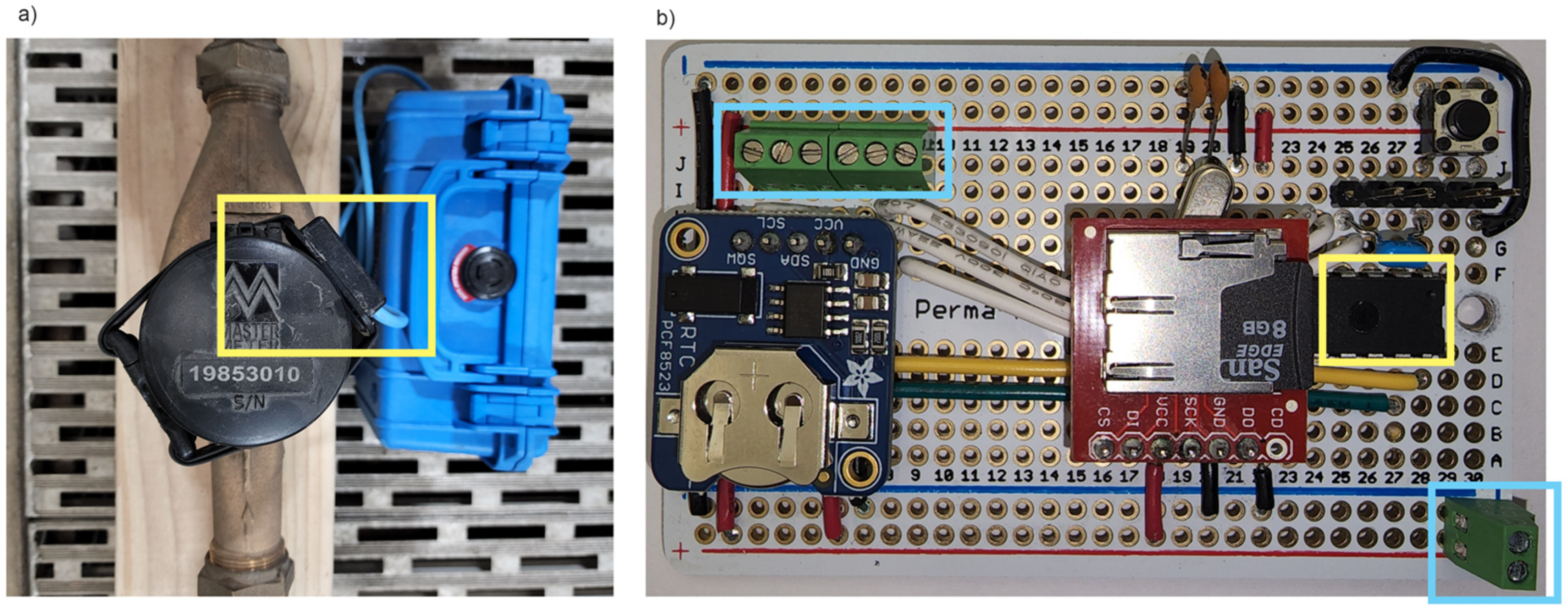
Full pulse resolution water use data were collected using the Pulse-Datalogger [18], which is a device designed specifically for this application. The Pulse-Datalogger builds on hardware previously developed by the authors [3,5] and measures the magnetic field outside of a magnetically driven water meter’s register, similar to devices used in past studies. In addition to a magnetometer sensor (LIS3MDL), the Pulse-Datalogger is composed of a microcontroller (ATMEGA328P chip), a Micro SD card, and a real-time clock (RTC). Figure 1 shows the Pulse-Datalogger deployed and the datalogging board. Most water meters operating today are not capable of collecting and storing sub-minute resolution water use data due to power and data volume limitations and because they were not designed or programmed to do so. These meters were designed to report aggregated volumes at periodic intervals, primarily for billing purposes. Therefore, studies collecting high resolution data have relied on datalogger devices that operate on top of existing meters and temporally aggregate data in an effort to extend the battery or data storage capacity of such devices to a short number of weeks (usually between 1 and 6 weeks of continuous deployment).
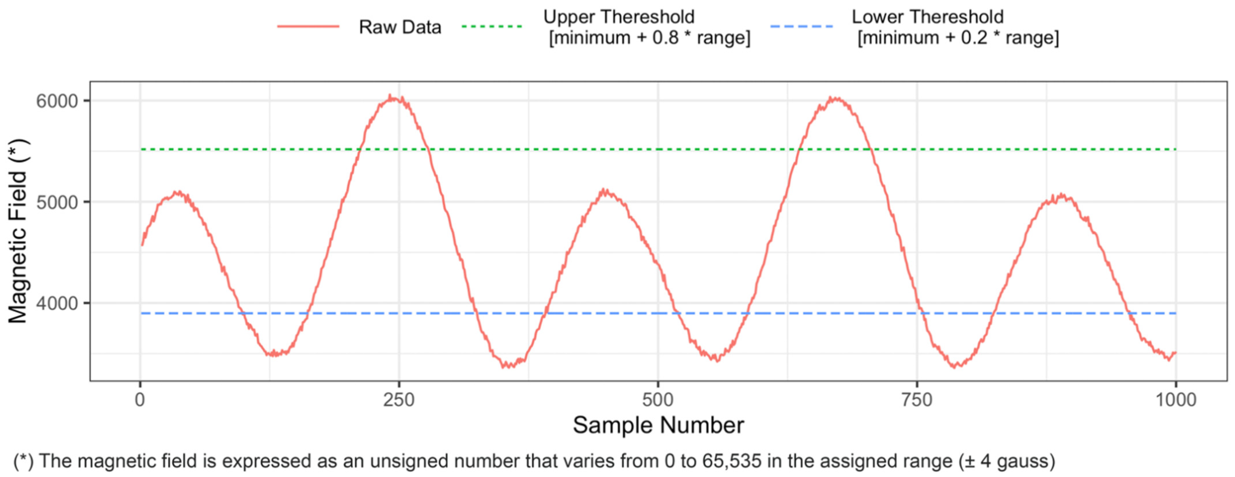
The Pulse-Datalogger was developed to capture data at the full pulse resolution by recording the time between each magnetic pulse. To accomplish this, we minimized power consumption and computation time by moving pulse recognition off the microcontroller (as is commonly done) and onto the magnetometer sensor. Under this approach, the Pulse-Datalogger can collect full pulse resolution data and match the highest observed deployment autonomy of similar dataloggers that record temporally aggregated data (i.e., approximately 5 to 6 weeks of continuous operation). A two-threshold approach (upper and lower) is used by the device to register pulses when the observed magnetic signal goes below the lower and subsequently above the upper threshold. Thresholds are defined by briefly (<1 min) running water through the meter after installing the device and recording the maximum and minimum magnetic field values observed in this period. The upper and lower thresholds are then set as a fraction of the maximum and the minimum recorded, as shown in Figure 2. The coefficients (0.8 and 0.2) used in threshold definition were calibrated under controlled conditions at the Utah Water Research Laboratory for the meter brands and sizes installed at Sites 1 and 2.
The microcontroller spends most of its time in a sleep state, only waking up when it receives an interrupt from the magnetometer or RTC. On an interrupt from the magnetometer (when a pulse is detected), the microcontroller computes the time since the last pulse and writes that to the Micro SD card. On an interrupt from the RTC (scheduled every day at midnight), the microcontroller restarts its internal clock to reduce time drift and starts logging in a new file. The firmware and hardware design of the Pulse-Datalogger are open source and publicly available on GitHub [18].
The Pulse-Datalogger outputs a comma separated values (CSV) file including a three-line header with information about (1) Date, a datetime value including the date and time in format “Year/Month/Day Hour:Minute:Second” indicating when data logging started; (2) Site, a 3 digit numerical identifier used to keep track of where the logger is installed; and (3) ID, a datalogger identifier (three-digit numerical) used to identify the datalogger. The Pulse-Datalogger records a single variable; time since last pulse (in ms) where the first value indicates time since the datetime included in the header. Raw data were then formatted, adding a date/time stamp to facilitate subsequent analyses and resulting in a CSV file containing two columns—the date/time stamp and the time since last pulse. The raw and formatted data files are publicly available in the HydroShare repository [19] in the RawPulseData and PulseData_Processed folders, respectively. The raw and formatted data collected are referred to as “pulse data” from this point forward. All data were collected between 11 February and 15 April 2022 when no outdoor water use was happening; therefore, only indoor water use was observed.
To verify the quality of the full pulse resolution data, the volume read by the Pulse-Datalogger was compared with the volume computed from manual readings of the meters’ registers conducted sporadically during deployments to ensure the accuracy of the data collected. The Pulse-Datalogger records water use on top of an existing meter by counting the revolutions of a spinning magnet inside the meter where the movement of the magnet is actuated by a fixed volume of water flowing through the meter. Thus, the maximum accuracy that can be obtained by the Pulse-Datalogger is that of the meter on which it is installed (i.e., the Pulse-datalogger and the meter’s register use the same measurement element inside the meter and should record the exact same volume). At Site 2, all data were collected in a single deployment (from 29 March 2022 to 15 April 2022). All data collected in this deployment were accepted for this study as the percent error of the volume recorded by the Pulse-Datalogger when compared to the manual meter readings was less than 0.1%. At Site 1, multiple data collection periods were needed (the start and end of each data collection period are available in HydroShare [19]). The largest error observed for deployments at Site 1 was 1.5%. During controlled laboratory experiments, the maximum error observed was less than 0.5%.
To fully explore event features and to facilitate our ability to identify and classify individual events in the data, we needed a set of labeled events with known types. Labeled events were generated in two ways. First, occupants of the two homes were asked to label a subset of individual water use events by recording the event type and start time using a cellphone application. Table 2 shows the total number and type of user labelled events. Second, we conducted a controlled experiment at Site 1. In this experiment, a set of individual faucet, toilet, shower, and bathtub events were recorded without any other end use occurring simultaneously. Each individual event type was repeated sequentially at least ten times for each fixture in the home, waiting at least 30 s between event repetitions and two minutes when switching fixtures. Showers, bathtubs, and faucets were kept running for at least 30 s, and toilets were flushed normally. Repetitions were performed to provide information about the variability in event feature values. To ensure the quality of the full pulse resolution data collected during the controlled experiment, we manually read the water meter’s register at Site 1 at the beginning and end of the experiment, calculated the volume of water used, and compared it with the volume read by the Pulse-Datalogger. We observed a percent error of less than 0.05%. The user labeled events and the controlled experiment event data are also available in the HydroShare repository [19].
2.3. Data Analyses
To evaluate the impact of the temporal resolution on event features and our ability to identify end uses of water, we aggregated the full pulse resolution data collected into the following temporal resolutions (selected from past studies): 1 s, 4 s, 5 s, 10 s, 15 s, 30 s, and 1 min. Data for all temporal aggregations evaluated have a start date/time of midnight on the first day of data available for each site, and subsequent timestamps were generated by adding the temporal resolution to this date and time. Given that water use events begin and end at random times, the exact date/time at which temporal aggregation intervals begin may affect the features calculated for some individual events. However, for consistency of our analyses, we began all time aggregated data at midnight.
Table 3 lists the features and data temporal resolutions used in several past studies that developed methods for end-use disaggregation and classification based on single point water use measurements. Some features (number of vertices, mode flow rate, shape) are commonly computed after filtering the data to remove oscillations from the flow trace data. The filtering technique may vary depending on the temporal resolution of the data and the event features to be calculated. The main function of these features is the identification of single and overlapping events, disaggregation of overlapping events into single events, and classification of single events into end-use categories.
We compared the impact of data temporal resolution on the number of events detected for each site and the main features obtained for the same events across the selected temporal resolutions. Additionally, we inspected user-labeled events to illustrate how the temporal resolution impacts event features beyond those tabulated and to investigate additional event features that can only be extracted from full pulse resolution data. We observed the impact of the temporal resolution on parameters included in Table 3 that can be computed without filtering data or disaggregating overlapping events.
3. Results and Discussion
3.1. Separation of Events
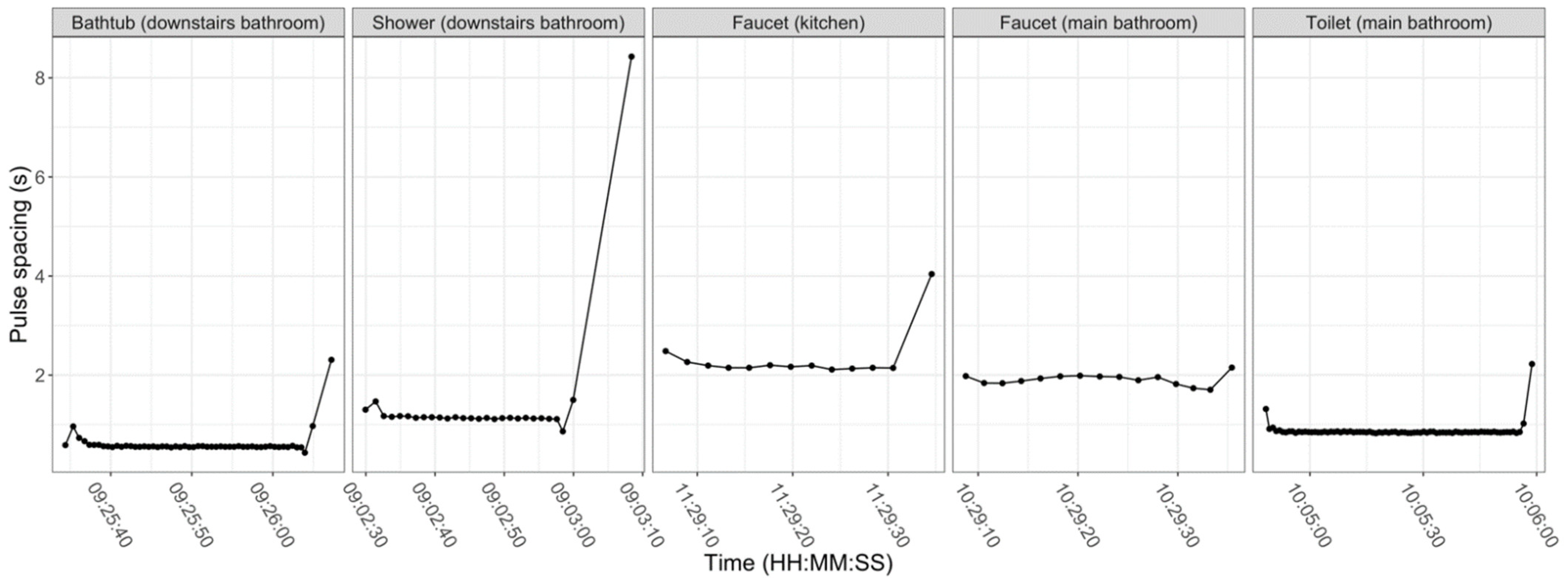
Analyses of the controlled experiment pulse data indicated there are delayed or trailing pulses happening at the end of each event that need to be counted as part of the event (Figure 3). After examining 132 events from the controlled experiment, we observed that only in three cases did these pulses happen more than 9 s after the previous pulse. Therefore, we adopted 9 s as the threshold to separate events in the pulse data (i.e., if a pulse happens more than 9 s after the previous pulse, a new event is initiated). For time aggregated data derived from the pulse data with temporal resolutions that were larger than 9 s, an event was ended when a value of 0 pulses was recorded. For 1 s, 4 s, and 5 s time aggregated data, we used 9, 8, and 10 s as the threshold to separate events, respectively. In past studies [3,5,16,17], event definition did not include these trailing pulses as events were terminated at the first time-step for which there were no recorded pulses. For example, we labeled single-pulse events as unclassified in our past studies and identified a large number of them (79% of all indoor events [17]) across all participant sites. It is unclear whether such events have been labeled as leaks by other authors; however, the pulse data shows that trailing pulses are part of the preceding event and have been misrepresented in the past. Single pulse events can also result from brief end uses or leaks.
The optimal value of the threshold used to separate events may vary for different sites depending on pipe pressure and fixtures characteristics (e.g., year, model) or types. If choosing a smaller value (that does not capture trailing pulses), single-pulse events must be identified and included in preceding events when they are determined to be resulting from such events. In the opposite case (selecting a value larger than optimal), a method for separating events occurring close together must be defined and applied to avoid combining multiple events into one. Table 4 shows the number of events detected at each temporal resolution using the thresholds described above. The number of detected events decreases as the temporal resolution decreases. This will affect estimation of event features and all frequency analyses conducted.
Further analysis showed that if we separate events from 4 s data when a value of 0 pulses is observed as we did in our past studies [3,7,16,17], the total number of events recorded for Site 1 and 2 is 1928 and 3377, and the number of single-pulse events increases to 489 and 1266, respectively (as compared to the numbers in Table 4). A similar result is observed by conducting the same analysis on 5 s data, also used in past studies [14]. When collecting 10 s data and separating events [10,11], the aggregation interval is long enough that trailing pulses are included within the last time interval of the event. However, with 10 s data, we observed only approximately 90% and 77% of the events detected with the pulse data, at Sites 1 and 2 respectively, which will also affect frequency estimates and calculation of event features. Collecting data at coarser temporal resolutions (30 s or 1 min) further reduces ability to detect individual events. At these coarser temporal resolutions, we observed more consecutive events being aggregated into single events as water use never returns to zero (the criteria used to separate events).
3.2. Analysis of Event Features
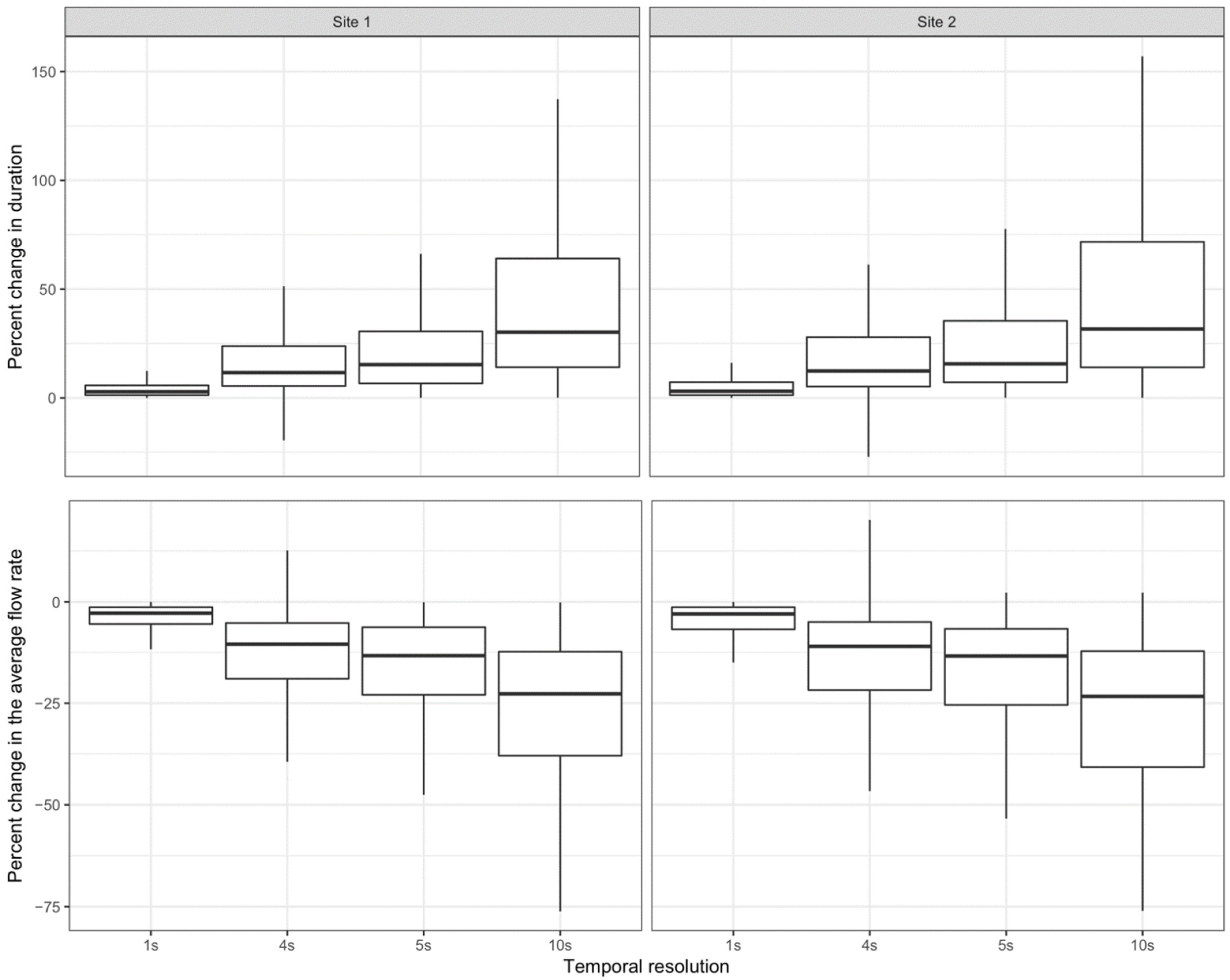
Figure 4 shows the percent change in the duration of events and the average flow rate for each event derived from pulse data versus the four smallest temporal resolutions analyzed (1, 4, 5, and 10 s). Data at temporal resolutions larger than 10 s were not further analyzed as the number of events detected already indicates these data are not suitable for end-use analyses without more advanced event separation and identification techniques. Single-pulse events were not included in these analyses. Events were matched based on their start date and time (pairing an event identified from time aggregated data with the closest event from the pulse data). Events with start time differences larger than 1.5 times the temporal resolution of the data were removed from the analysis. By doing this, we ensure we are comparing the same event across all temporal resolutions and removing the effect of aggregated consecutive events. Comparing an aggregated event with multiple single components would result in larger differences than those observed in Figure 4. The volume of the events analyzed will not change in most cases as our constraints are aimed at identifying the same event across all temporal resolutions, and the number of pulses for each event does not change, regardless of the temporal resolution at which pulses are recorded.
The calculated duration of events increases as the temporal resolution decreases. The median percent change in duration when collecting 10 s data is larger than 30%, while the same value for events identified from 1 s resolution data is approximately 3% for both sites analyzed. The average flow rate of events decreases as the temporal resolution decreases. This has important implications when assessing the performance of individual fixtures using the average flow rate (as is commonly done for faucets or showerheads). Durations calculated from lower resolution data will be biased high and will not accurately reflect behavior. Flow rates will be biased low and will not be representative of the true performance of fixtures.
Furthermore, there are differences in the number of data points collected for each event (e.g., an event that lasts 11 s will have 11 data points at 1 s resolution and 2 data points at 10 s resolution). This disparity will impact estimates of event features such as the mode flow rate, median flow rate, number of vertices in the shape of the event, and any other features depending on frequency or shape of an event. A smaller number of data points will produce less information that can be used to identify single or overlapping events, split overlapping events into single components, and calculate unique features that can be extracted for classification purposes. The number of data values recorded for each event is also influenced by the volumetric pulse resolution of the meter. A larger value for volumetric resolution (L/pulse) will result in fewer pulses.
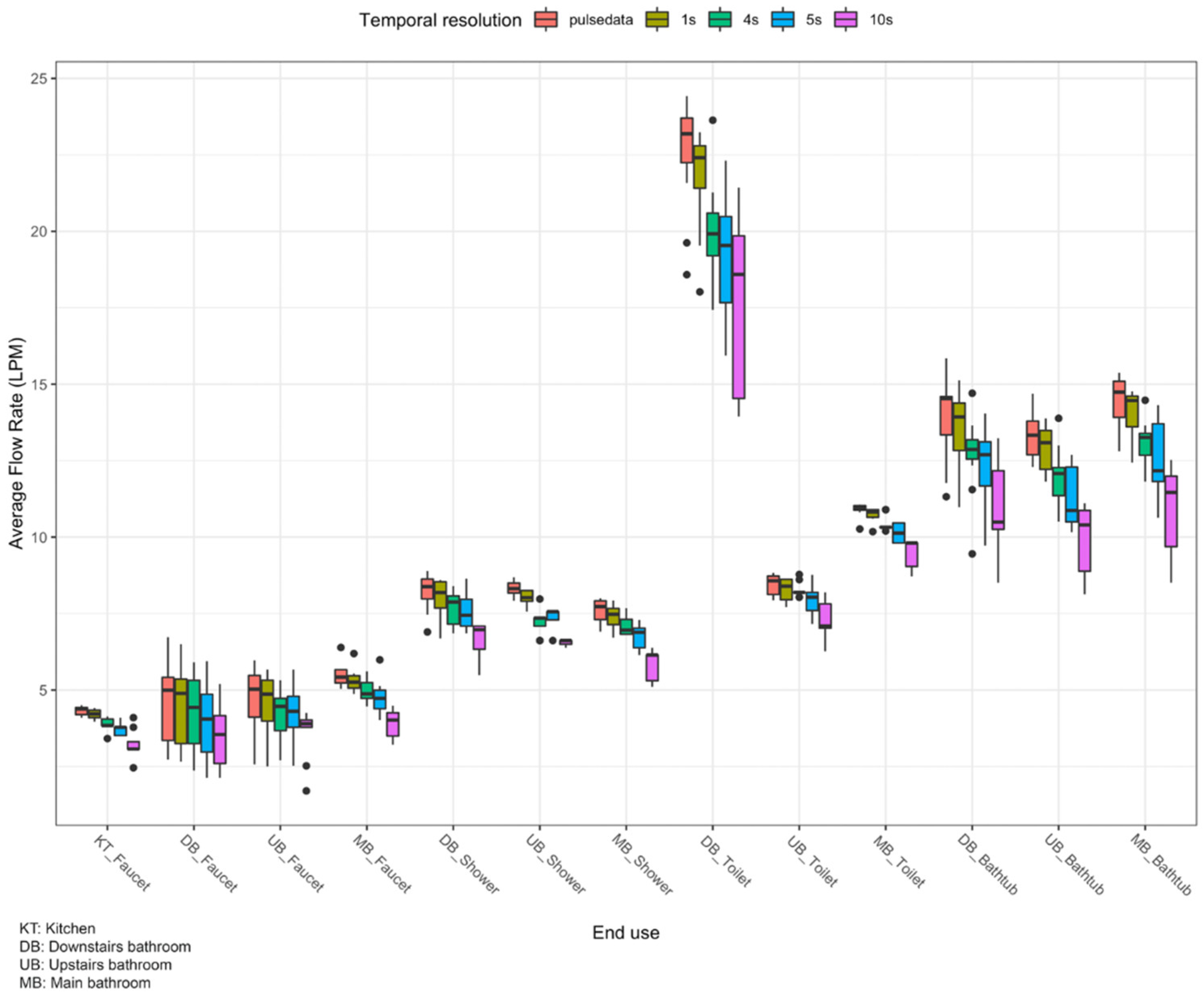
Figure 5 presents the distributions of average flow rate values calculated from the controlled experiment events. Our prior analyses of water use event data indicate that the most distinctive features used for event classification are duration and average flow rate. Mode and maximum flow rate are highly correlated (between 0.9 and 1) with the average flow rate. Event volume, which is a multiple of duration and average flow rate, is highly correlated with duration. Figure 5 indicates that, at Site 1, it is possible to differentiate end uses based on the average flow rate of events alone at most temporal resolutions given that the distributions of average flow rate values for different event types largely do not overlap (distributions of average event flow rates do overlap for 10 s data). Additionally, mechanical events of the same type (e.g., toilets, clothes washer, dish washer) will have similar duration. For showers and faucets, duration will exhibit larger variability. The median average flow rate for the upstairs bathroom shower at Site 1 estimated from pulse data is 8.38 LPM versus 6.62 LPM when estimated from 10 s data. The duration of events (with the exception of toilets) was fixed during the controlled experiment; therefore, duration was not analyzed for these events.
Figure 6 shows the distributions of average flow rate and duration values for events that were manually labeled by residents at both sites. There are distinct combinations of flow rate and duration corresponding to each end use at both sites for almost all temporal resolutions evaluated, suggesting that these features could be sufficient to classify individual events. However, identifying end uses at the fixture level (i.e., the specific fixture using water) seems more plausible at higher temporal resolutions. For example, separating half bathroom and downstairs bathroom events (toilets or faucets) for Site 2 appears possible for pulse data and 1 s data, but challenging at other temporal resolutions as the flow rates overlap for temporal resolutions lower than 1 s. Residents of both sites were instructed to label only single use events (i.e., no other use was happening at the same time). We did not observe fundamental differences in the data, or event features, from these two sites, despite their different characteristics (Table 1), as the events presented in Figure 6 suggest. This indicates pulse data collection can be generalized for properties with different meter types and water fixture technologies.
3.3. Event Features Extracted from Pulse Data
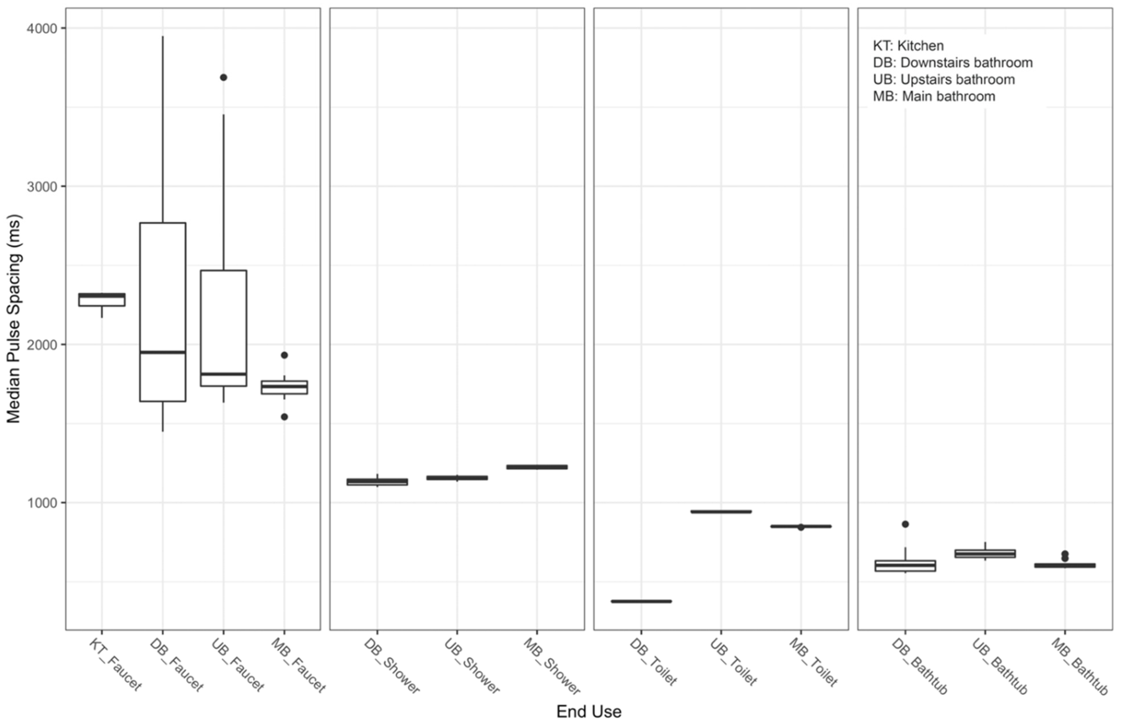
To date, features used for classifying events have all been calculated from time aggregated data. As our results above show, depending on the data collection interval, features calculated from time aggregated data may or may not discriminate events. Pulse data provide the opportunity to extract new features that may be more discriminating and thus make classification easier and more accurate. The previous analyses focused on calculating features that could be compared across multiple temporal resolutions; however, the pulse data and features calculated from it can also be used to classify events. For example, Figure 7 shows that median pulse spacing can be used to classify individual events following simple rules (e.g., any event with a median pulse spacing larger than 1400 ms is a faucet event). Such rules may even be able to discriminate individual fixtures (e.g., any event with a pulse spacing less than 500 ms is a flush of the downstairs bathroom toilet). Similar rules with different values could be defined for each household, which would facilitate data processing and classification, particularly in real-time applications. While the specific rules used to classify events may be unique to each site and its fixtures, we anticipate that similar rules can be implemented for any residential household, as long as fixtures operate at different flow rates and have different duration, which is normally the case.
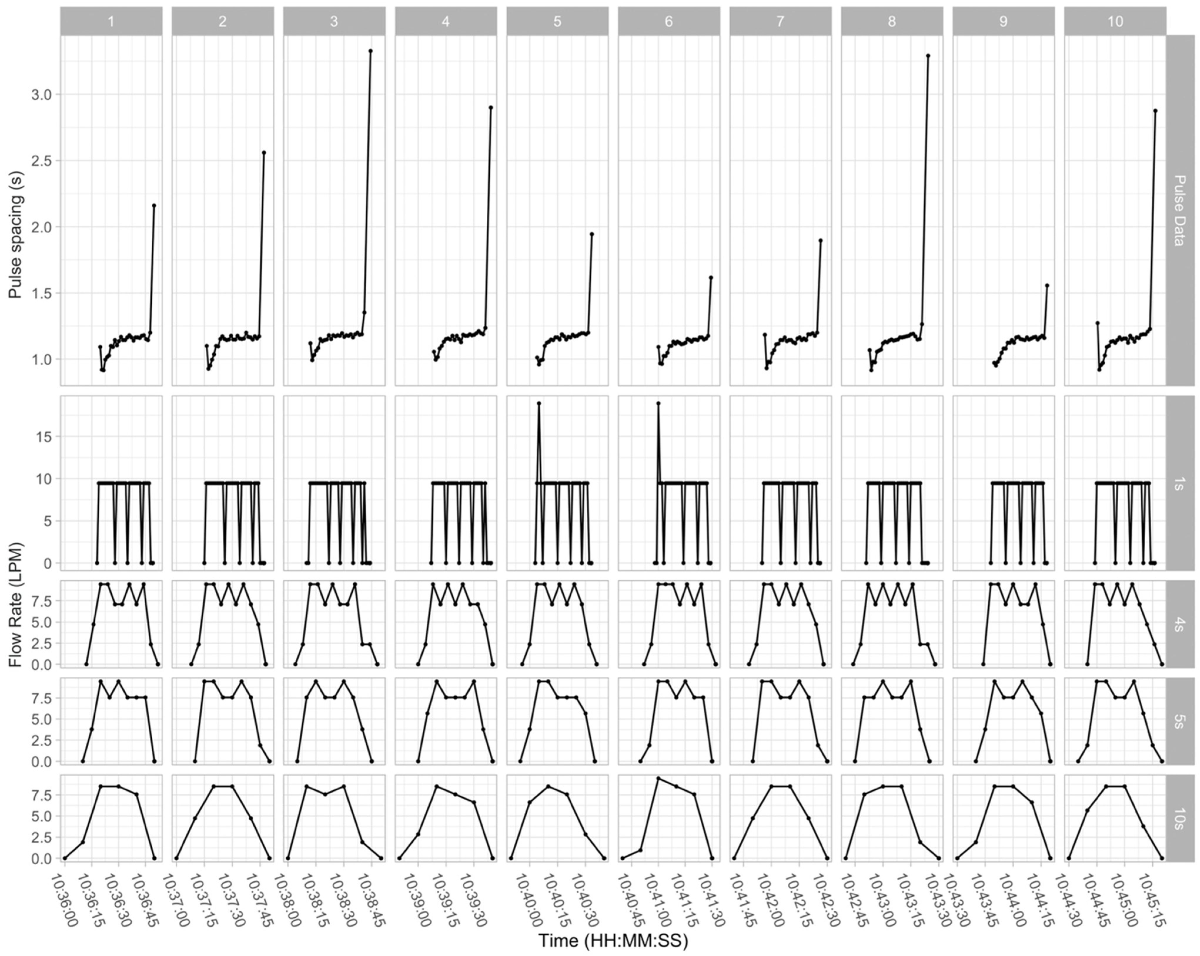
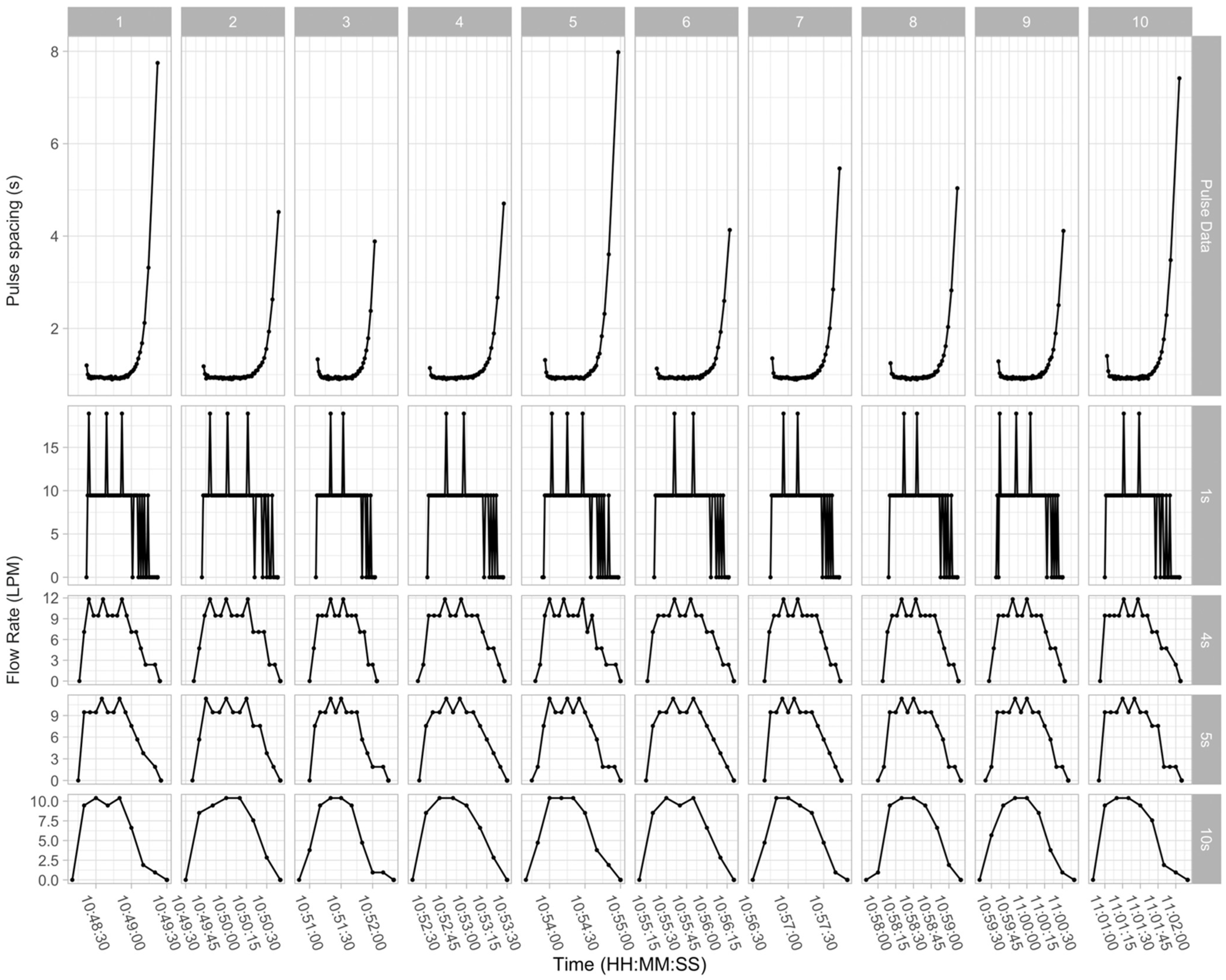
Another pulse data feature that may assist in the classification process is the shape of events. For example, all shower events in Figure 8 (events from the same fixture) have a similar starting and ending pattern when observing pulse data. Figure 9 shows pulse and temporally aggregated data for 10 flushes of the same toilet. The pulse data shape is consistent for repetitions of the same event, and distinctive for each fixture. While temporally aggregated data captures high and low flow rate phases within each event, it does not provide a distinctive signature that can be used for events classification (Figure 8 and Figure 9). Analyzing the pulse spacing for the first and last n values of each event may assist in the classification process and support fixture level classification. We found that these patterns are different but exist in the pulse data for all fixtures analyzed for both sites.
3.4. Analysis of Overlapping Events
Section 3.3 demonstrates how pulse data can facilitate individual event classification. However, overlapping events typically require additional processing as the flow trace must be disaggregated into single components that can later be classified. The frequency with which overlapping events occur is determined by the number of occupants of a site, their schedule, and water use preferences. In our analysis of 4 s data collected at 31 residential properties [21], we found that approximately 10% of all the events identified were overlapping events, and they represented approximately 40% of the volume recorded. However, data were collected during summer and winter months and include irrigation events that are long in duration with high probability for overlapping [17]. On average, after applying a splitting procedure that we designed to disaggregate overlapping events, each identified overlapping event produced 4.4 single events. Again, the large number of single events per overlapping event largely resulted from long duration irrigation events. The large volume comprised of overlapping events makes their disaggregation and classification essential in order to provide an accurate picture of residential water use. However, identifying and splitting overlapping events is dependent upon the temporal resolution of the data, and classifying events resulting from the decomposition of overlapping events is challenging, as these events will have different features depending on both the temporal resolution of the data and the algorithm or method used to separate them.
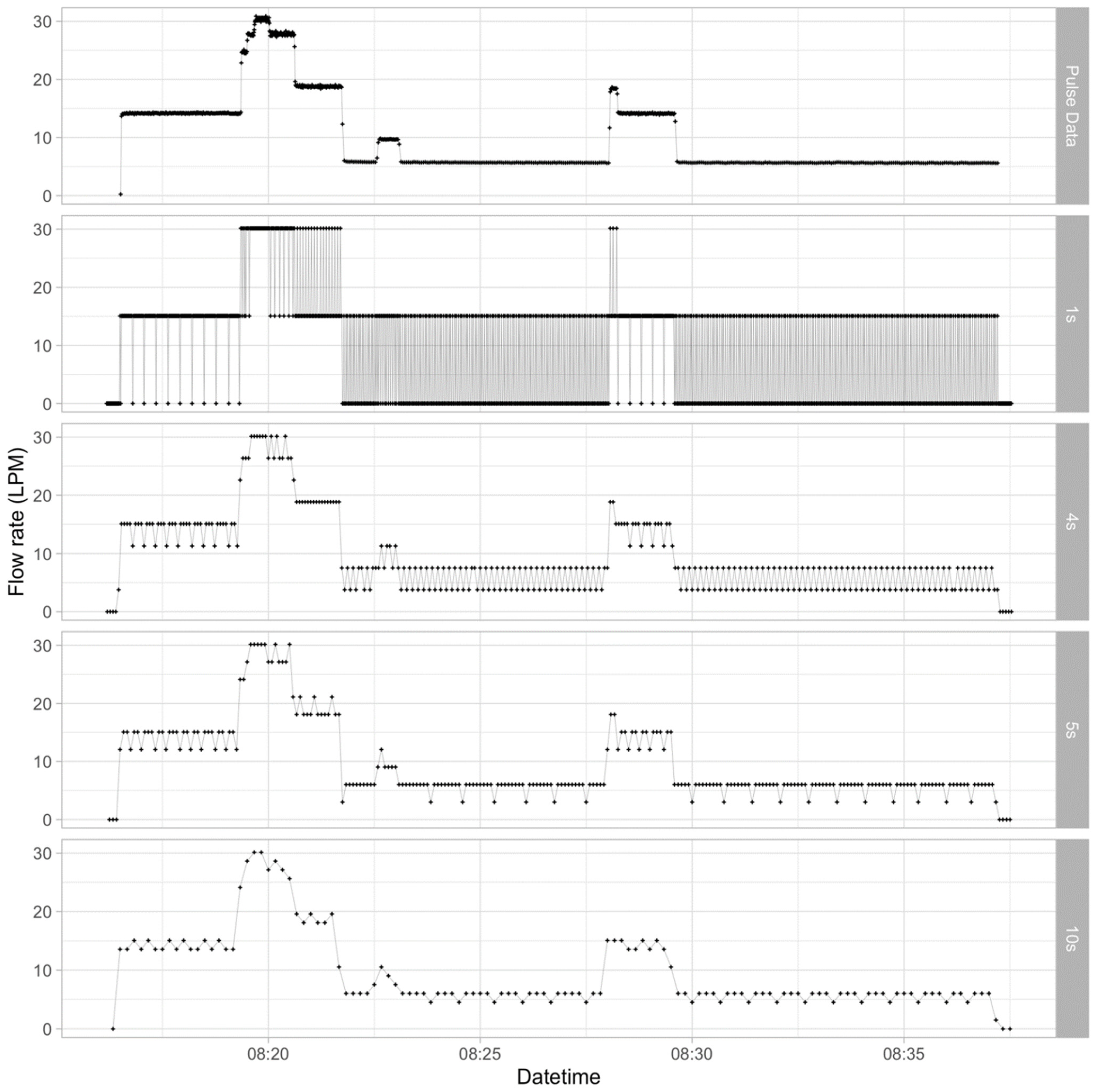
Figure 10 shows the flow rate of an overlapping event composed of multiple single events observed at Site 2 The oscillations in flow rate observed at all temporal resolutions other than the pulse data reinforce the need for applying filtering techniques to smooth the flow trace for time aggregated data prior to calculating event features. These oscillations are a result of the volumetric pulse resolution of the meter (i.e., only a discrete number of pulses can be counted in any time interval) and the data recording interval (i.e., pulses are not always evenly spaced in time at a factor of the temporal resolution). The oscillations are largest for 1 s data and decrease for 10 s data by sacrificing flow trace details. Filtering can be used to address these oscillations but may remove the ability to observe low flow rate events overlapping other end uses and may also mask features related to the original shape of the event that are important for fixture level classification.
At certain temporal resolutions, some events and event features cannot be seen. For example, the short low flow rate event observed after 8:22 a.m. (Figure 10) is of similar magnitude to the oscillations observed in 4 and 5 s data and would likely be ignored at these resolutions, while for 10 s data the event is not distinguishable. It would not be possible to separate such events without building an overly sensitive model that may erroneously separate some single events given that flow rate changes also occur in some single events. In our prior work, the number of overlapping events increased during summer months when irrigation was occurring, as irrigation events tend to have longer duration than indoor events. Therefore, the importance of collecting data at a sufficient temporal resolution to identify and separate overlapping events increases during these months. The pulse data shown in Figure 10 are clearly superior to the time aggregated data in recording the complex shape of this overlapping event and will make identification and separation of overlapping events easier and more accurate. The steady behavior of pulse data opens the possibility for event disaggregation without filtering, which would facilitate more accurate classification of the single, disaggregated events as their original features can be preserved.
3.5. Data Volumes
Collecting data at higher temporal resolutions has several data management implications related to the data volume generated [7]. These result from general needs to record (e.g., locally on a datalogger), transmit (e.g., over a telemetry network), store and organize (e.g., in a database), manage, and analyze the data for potentially many sites. Commonly, high temporal resolution data consist of two recorded variables, a date/time stamp identifying the data aggregation interval and the number of pulses and/or volume of water that has passed through the meter during that interval. Given the high temporal resolution of the data, the volume of generated data can grow quickly. One strategy for reducing the volume of data generated is to record only non-zero values. Another strategy is to record a beginning date/time and then record only water usage without time stamps (assuming that the data are regularly spaced). The pulse data we collected consist only of numeric values for the time since the last pulse, which is similar to the second option. The pulse data are dense during times when water use is occurring, but no values are recorded when flow through the meter is zero.
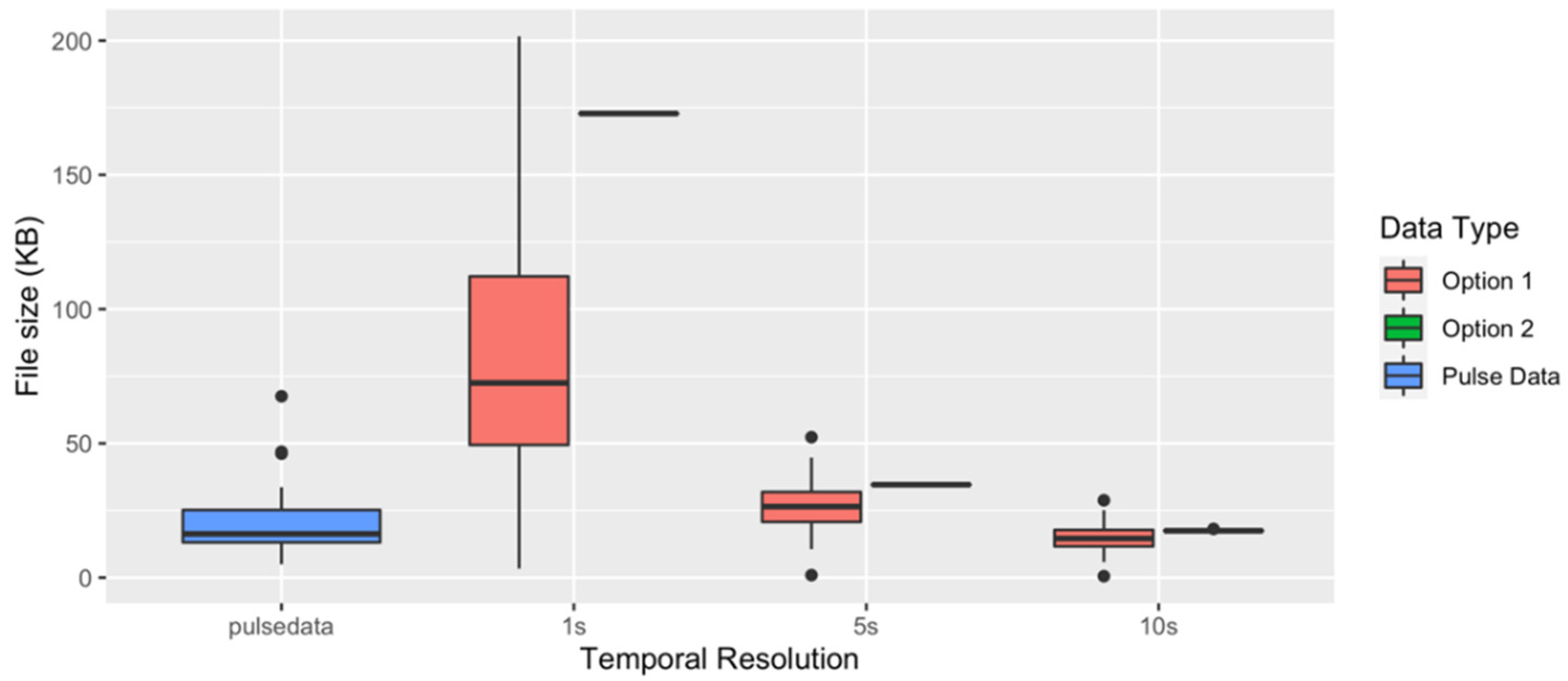
To assess the impact of these data collection and recording strategies, we compared daily file sizes generated from pulse data recorded on our datalogger versus daily files for time aggregated data of different temporal resolution using both possible options: (1) with time stamps and no zeros; and (2) with zeros without time stamp (Figure 11). We used full days of data collected and generated daily CSV files for each temporal resolution.
It is expected that file sizes (for pulse data and option 1) will be larger during summer months (or times of higher water use), as file sizes will increase as water use does. Pulse data preserves more detail about events and generates equal or lesser volumes of data when compared with temporal resolutions that would allow end-use classification. Recording data with full pulse resolution does not increase the data volume generated when compared with time-aggregated data up to a 10 s temporal resolution.
4. Conclusions
In this paper, we presented analyses and comparison of residential water use data at different temporal resolutions in comparison to full pulse resolution data collected using a specialized datalogger. To answer our first research question about how the temporal aggregation interval of recorded data affects ability to identify, classify, and calculate attributes or features of individual events, we demonstrated that as data temporal resolution decreases, the number of detected end-use events decreases. We also showed how estimates of event features and the shape of overlapping events were impacted with decreasing temporal resolution (e.g., as data temporal resolution decreases, estimated event duration increases and average flowrate decreases). Our results show that temporally aggregating pulse data reduces ability to accurately estimate event features and generates oscillations in the data that require filtering techniques to remedy. However, those same filtering techniques can remove or mask important event features that could be used for event classification.
Regarding the volume of data generated, the final component of our first research question, pulse data captured a larger, and more accurate, number of events at each of the sites without negatively impacting the volume of data generated when compared to time aggregated data collected at temporal resolutions most suitable for end-use identification, disaggregation, and classification (i.e., up to 10 s resolution). Additionally, when overlapping events occur, time aggregation of the data can mask the features of such events, whereas pulse data provide a much cleaner trace that would better facilitate disaggregating overlapping events.
We observed that the values of features calculated for events changed as the temporal resolution decreased, which will negatively impact any classification algorithm or methodology that uses those features. Key event features, such as the mode flow rate, the average flow rate, and the duration vary as the temporal resolution decreases leading to more overlap in the distributions of these values and less power in using these features to discriminate event types (e.g., for classification). These variations in the number of identified events and their features have implications on the accuracy of any analyses based on frequency or event features. For example, estimates of the technical performance of water using fixtures are impacted by data temporal resolution and would best be done using pulse data.
Regarding our second research question, the pulse spacing values within events provide unique features that could be used to more accurately identify and classify end-use events. In our controlled experiment, events of different types exhibited unique behavior at the beginning and end of events, and the median pulse spacing for events of different types shows great promise as a discriminating feature for classification purposes. These results also argue for using meters with higher pulse resolution (i.e., smaller volume per pulse), which would provide greater detail in the trace of individual events and reduce the likelihood of “zero-pulse” events (i.e., events having volume smaller than the pulse resolution of the meter) that are registered as part of the subsequent event. While it may not be practical to replace existing meters for this reason, and in some cases may be impossible given requirements for safe and accurate meter operation at higher flowrates (e.g., those seen at homes with automated irrigation systems), the pulse resolution of the meter may be an important consideration when installing new or in retrofitting existing meter networks.
While we evaluated data from only two single family residential properties, the data were similar for both newer, single-lever-type fixtures and older dual-knob-type fixtures, indicating that the uniqueness of event features from different water use fixtures we observed in the pulse data (e.g., flow rate, pulse spacing, event shape, and unique behavior at the beginning and ending of events) will exist across water using fixtures at any property. Thus, collecting pulse data could provide generalized capability to not only provide temporally aggregated data for any existing operational purposes (e.g., regular billing) but can also provide more detailed information and discriminating event features for use in end-use studies. More discriminating features could, in turn, make end-use disaggregation and classification algorithms simpler and more computationally efficient. This could change smart metering technology by enabling more efficient computation of end-use information directly on the meter using edge computing techniques such as those demonstrated by Attallah et al. [5]. This would open the door for more real-time applications of the data, including customer feedback portals, in-home displays, and leak detection and alerting.
The benefits of pulse data are clearly illustrated here and warrant consideration in future data collection efforts. While differences in the volumetric pulse resolutions of different meter brands, models, and sizes will still exist, collecting full pulse resolution data would eliminate differences among data collected with different temporal resolutions, leading to greater standardization of data collection and analysis methods. Full pulse resolution data were superior in clearly identifying a larger number of end-use events, they contributed to more accurate and less ambiguous calculation of event features, they reduce or eliminate the need for data filtering prior to calculating event features, they more clearly capture the complexity of overlapping events, and they provide new event features that are highly discriminatory among events of different types—all without increasing the volume of data that have to be recorded, transmitted, stored, and analyzed. These benefits bring opportunities for smart-metering manufacturers to adopt similar data collection strategies which can lead to better information about water use, faster analytics, and more accurate user feedback.
Author Contributions
All authors contributed to the conceptualization of the work presented and in the selection of the methodology used. A.S.B.J. led hardware prototyping and firmware development with contributions from C.J.B.P. and J.S.H.; C.J.B.P. led the field data campaign, data management, and analysis with contributions from J.S.H. and A.S.B.J.; C.J.B.P. wrote the initial draft of the paper. J.S.H. and A.S.B.J. contributed to review and editing. J.S.H. provided project supervision and funding acquisition. All authors have read and agreed to the published version of the manuscript.
Funding
This research was funded by the United States National Science Foundation under grant number 1552444. Any opinions, findings, and conclusions or recommendations expressed are those of the authors and do not necessarily reflect the views of the National Science Foundation. Additional support was provided by the Utah Water Research Laboratory at Utah State University.
Institutional Review Board Statement
The study was conducted according to the guidelines of the Declaration of Helsinki, and approved by the Institutional Review Board of Utah State University (protocol code 9595 approved on 24 June 2020).
Informed Consent Statement
Informed consent was obtained from all subjects involved in the study.
Data Availability Statement
The designs for the Pulse-Datalogger, including the hardware parts list, firmware code, and related supplemental materials are publicly available in the GitHub repository for the project [18]. The anonymized data collected at each site and R scripts used to produce the results presented in this paper are published in the HydroShare repository [19].
Acknowledgments
We want to acknowledge and thank the owners of the residential homes that participated in the data collection campaign. We also acknowledge Nour Attallah’s contribution to the field data collection campaign and comments on the manuscript.
Conflicts of Interest
The authors declare no conflict of interest.
References
- Boyle, T.; Giurco, D.; Mukheibir, P.; Liu, A.; Moy, C.; White, S.; Stewart, R. Intelligent Metering for Urban Water: A Review. Water 2013, 5, 1052–1081. [Google Scholar] [CrossRef] [Green Version]
- Cominola, A.; Giuliani, M.; Castelletti, A.; Rosenberg, D.E.; Abdallah, A.M. Implications of Data Sampling Resolution on Water Use Simulation, End-Use Disaggregation, and Demand Management. Environ. Model. Softw. 2018, 102, 199–212. [Google Scholar] [CrossRef] [Green Version]
- Bastidas Pacheco, C.J.; Horsburgh, J.S.; Tracy, R.J. A Low-Cost, Open Source Monitoring System for Collecting High Temporal Resolution Water Use Data on Magnetically Driven Residential Water Meters. Sensors 2020, 20, 3655. [Google Scholar] [CrossRef] [PubMed]
- F.S. Brainard & Company Meter-Master. 2022. Available online: https://meter-master.com/product/model-100el-100af/ (accessed on 10 June 2020).
- Attallah, N.A.; Horsburgh, J.S.; Beckwith, A.S.; Tracy, R.J. Residential Water Meters as Edge Computing Nodes: Disaggregating End Uses and Creating Actionable Information at the Edge. Sensors 2021, 21, 5310. [Google Scholar] [CrossRef] [PubMed]
- Pastor-Jabaloyes, L.; Arregui, F.J.; Cobacho, R. Water End Use Disaggregation Based on Soft Computing Techniques. Water 2018, 10, 46. [Google Scholar] [CrossRef] [Green Version]
- Attallah, N.A.; Horsburgh, J.S.; Bastidas Pacheco, C.J. An Open-Source, Semi-Supervised Water End Use Disaggregation and Classification Tool. J. Water Resour. Plan. Manag. 2022. submitted for publication. [Google Scholar]
- Aquacraft Trace Wizard Description. 1996. Available online: http://www.aquacraft.com/downloads/trace-wizard-description/ (accessed on 15 June 2022).
- Nguyen, K.A.; Stewart, R.A.; Zhang, H.; Sahin, O. An Adaptive Model for the Autonomous Monitoring and Management of Water End Use. Smart Water 2018, 3, 5. [Google Scholar] [CrossRef] [Green Version]
- DeOreo, W.B.; Mayer, P.W.; Dziegielewski, B.; Kiefer, J.; Foundation, W.R. Residential End Uses of Water, Version 2; Water Research Foundation: Denver, CO, USA, 2016; ISBN 9781605732350. Available online: https://www.waterrf.org/research/projects/residential-end-uses-water-version-2 (accessed on 15 March 2022).
- Mayer, P.W.; DeOreo, W.B.; Optiz, E.M.; Kiefer, J.C.; Davis, W.Y.; Dziegielewski, B.; Nelson, J.O. Residential End Uses of Water; American Water Works Association: Denver, CO, USA, 1999. [Google Scholar]
- Heinrich, M. Water End Use and Efficiency Project (WEEP); Final Report; BRANZ: Judgeford, New Zealand, 2007. [Google Scholar]
- Suero, F.J.; Mayer, P.W.; Rosenberg, D.E. Estimating and Verifying United States Households’ Potential to Conserve Water. J. Water Resour. Plan. Manag. 2012, 138, 299–306. [Google Scholar] [CrossRef]
- Beal, C.; Stewart, R.A. South East Queensland Residential End Use Study; Final Report. 2011. Available online: http://www.urbanwateralliance.org.au/publications/UWSRA-tr47.pdf (accessed on 20 February 2022).
- Gato-Trinidad, S.; Jayasuriya, N.; Roberts, P. Understanding Urban Residential End Uses of Water. Water Sci. Technol. 2011, 64, 36–42. [Google Scholar] [CrossRef] [PubMed]
- Bastidas Pacheco, C.J.; Brewer, J.C.; Horsburgh, J.S.; Caraballo, J. An Open Source Cyberinfrastructure for Collecting, Processing, Storing and Accessing High Temporal Resolution Residential Water Use Data. Environ. Model. Softw. 2021, 144, 105137. [Google Scholar] [CrossRef]
- Bastidas Pacheco, C.J.; Horsburgh, J.S.; Attallah, N.A. Variability in Consumption and End Uses of Water for Residential Users in Logan and Providence, Utah, USA. J. Water Resour. Plan. Manag. 2022. submitted for publication. [Google Scholar]
- CIWS-Pulse-Logger. Available online: https://github.com/UCHIC/CIWS-Pulse-Logger (accessed on 3 May 2022).
- Bastidas Pacheco, C.J.; Horsburgh, J.S.; Beckwith, A.S., Jr. Supporting Data and Tools for “Impact of Temporal Resolution on Data for Quantifying Residential End Uses of Water”. HydroShare. 2022. Available online: https://doi.org/10.4211/hs.6625bdbde41c45c2b906f32be7ea70f0 (accessed on 16 May 2022).
- Deb, K.; Pratap, A.; Agarwal, S.; Meyarivan, T. A Fast and Elitist Multiobjective Genetic Algorithm: NSGA-II. IEEE Trans. Evol. Comput. 2002, 6, 182–197. [Google Scholar] [CrossRef] [Green Version]
- Bastidas Pacheco, C.J.; Attallah, N.A.; Horsburgh, J.S. High Resolution Residential Water Use Data in Cache County, Utah, USA. 2021. HydroShare. Available online: https://www.hydroshare.org/resource/0b72cddfc51c45b188e0e6cd8927227e (accessed on 16 May 2022).
Figure 1.
(a) Pulse-Datalogger installed on a 1 in Master Meter meter (the yellow rectangle shows the magnetometer sensor attachment on the meter’s register). (b) Datalogging board with: magnetometer sensor and battery connections indicated in the top and bottom blue rectangles, respectively; microcontroller highlighted in the yellow rectangle; micro SD card visible in the center of the board; and real-time clock visible on the left. In a deployment, the battery and datalogging board are enclosed in the blue box shown in panel (a).

Figure 2.
Sample data collected during the calibration period at Site 2 and upper and lower threshold definition. The x-axis represents approximately 6.5 s (the magnetic field is sampled at 155 Hz). For the type of meter available at Site 2 (1 in Neptune T-10) the Pulse-Datalogger was calibrated (thresholds set) to count only the highest peaks to reduce noise as the smaller peaks are not equally spaced.

Figure 3.
Pulse data for different Site 1 events from the controlled experiment. Each panel shows an individual event. The first value of each event was removed for visualization as it represents time since the previous event.
Figure 3.
Pulse data for different Site 1 events from the controlled experiment. Each panel shows an individual event. The first value of each event was removed for visualization as it represents time since the previous event.

Figure 4.
Percent change in the duration of events (top row) and average flow rate (bottom row) for all events at different temporal resolutions compared with events identified from pulse data.
Figure 4.
Percent change in the duration of events (top row) and average flow rate (bottom row) for all events at different temporal resolutions compared with events identified from pulse data.

Figure 5.
Distributions of average flow rate values for the controlled experiment events (Site 1) derived from pulse data and from data aggregated at different temporal resolutions.
Figure 5.
Distributions of average flow rate values for the controlled experiment events (Site 1) derived from pulse data and from data aggregated at different temporal resolutions.

Figure 6.
Distributions of average flow rate and duration values for events manually labeled by residents from data aggregated at different temporal resolutions and pulse data.
Figure 6.
Distributions of average flow rate and duration values for events manually labeled by residents from data aggregated at different temporal resolutions and pulse data.

Figure 7.
Distribution of median pulse spacing for all events from the controlled experiment at site 1.
Figure 7.
Distribution of median pulse spacing for all events from the controlled experiment at site 1.

Figure 8.
Pulse spacing and temporally aggregated data for the downstairs bathroom shower events from the controlled experiment events at Site 1. Each column (1 to 10) shows a different event.
Figure 8.
Pulse spacing and temporally aggregated data for the downstairs bathroom shower events from the controlled experiment events at Site 1. Each column (1 to 10) shows a different event.

Figure 9.
Pulse spacing and temporally aggregated data for the downstairs bathroom toilet events from the controlled experiment events at Site 1. Each column (1 to 10) shows a different event.
Figure 9.
Pulse spacing and temporally aggregated data for the downstairs bathroom toilet events from the controlled experiment events at Site 1. Each column (1 to 10) shows a different event.

Figure 10.
Pulse data and time aggregated data converted to flowrates at different temporal resolutions for a single overlapping event at Site 2. Event start date and time: 2022-04-02 08:16:30.910 MT, event duration: 20.6 min.
Figure 10.
Pulse data and time aggregated data converted to flowrates at different temporal resolutions for a single overlapping event at Site 2. Event start date and time: 2022-04-02 08:16:30.910 MT, event duration: 20.6 min.

Figure 11.
Comparison of distributions of daily CSV file sizes generated from data collected at different temporal resolutions versus pulse data files. Option 1 refers to data with time stamps but no zero values. Option 2 refers to data with zeros but no time stamp. Pulse data does not contain a time stamp for each recorded value.


Table 1.
Main characteristics of the two sites where full pulse resolution data was collected.
| Site | Length of Record (Days 1) | Number of Occupants | Meter Brand | Meter Size (in) | Volumetric Pulse Resolution (L/Pulse) | Year Built | Number of Bathrooms 2 |
|---|---|---|---|---|---|---|---|
| 1 | 26 | 4 | Master Meter | 1 | 0.16 | 2006 | 3 |
| 2 | 18 | 2 | Neptune | 1 | 0.25 | 1968 | 2 ½ |
1 Days with partial records are counted as 1 day. There are 8 days with partial record at Site 1 and 2 days with partial record at Site 2.; 2 A half-bathroom consists of a sink and a toilet.
Table 2.
Summary of user labeled events by site and end use. The events labeled by participants represent only a small subset of all the events occurring at each site.
Table 2.
Summary of user labeled events by site and end use. The events labeled by participants represent only a small subset of all the events occurring at each site.
| Site | Total Labeled Events | Shower | Faucet | Toilet | Bathtub | Clothes Washer | Dishwasher |
|---|---|---|---|---|---|---|---|
| 1 | 89 | 17 | 46 | 17 | 3 | 3 | 3 |
| 2 | 92 | 10 | 36 | 26 | 0 | 10 | 10 |
Table 3.
Temporal resolution, event features, and broad methodology for end-use classification methods.
Table 3.
Temporal resolution, event features, and broad methodology for end-use classification methods.
| Authors | Temporal Resolution (s) | Event Features | Broad Methodology |
|---|---|---|---|
| Attallah et al. [7] | 4 | Volume; duration; average, mode, maximum, and root mean square flow rate, shape | Low pass filtering, supervised classification |
| Nguyen et al. [9] | 10 | Volume; duration; average and maximum flow rate; shape | Decision tree, dynamic time warping, self-organizing map, hidden Markov model |
| Pastor-Jabaloyes et al. [6] | 3, 0.02 | Volume; duration; average and maximum flow rate; shape | NSGA-II [20] filtering, unsupervised classification |
| De Oreo et al. [8] | 10 | Start and end time; duration; volume; average, maximum, and mode flow rate | Manual and visual inspection by an analyst assisted by a decision tree algorithm |
Table 4.
Number of events identified at each site for different temporal resolutions.
| Site | Temporal Resolution (s) | Number of Events Detected | Single Pulse Events | Events with More Than One Pulse |
|---|---|---|---|---|
| 1 | Pulse data | 1605 | 225 | 1380 |
| 1 | 1590 | 210 | 1380 | |
| 4 | 1578 | 203 | 1375 | |
| 5 | 1536 | 166 | 1370 | |
| 10 | 1513 | 153 | 1360 | |
| 15 | 1401 | 132 | 1269 | |
| 30 | 1158 | 86 | 1072 | |
| 60 | 960 | 55 | 905 | |
| 2 | Pulse data | 2118 | 590 | 1528 |
| 1 | 2072 | 554 | 1518 | |
| 4 | 2054 | 483 | 1571 | |
| 5 | 1878 | 355 | 1523 | |
| 10 | 1797 | 319 | 1478 | |
| 15 | 1648 | 272 | 1376 | |
| 30 | 1373 | 184 | 1189 | |
| 60 | 1072 | 125 | 947 |
Publisher’s Note: MDPI stays neutral with regard to jurisdictional claims in published maps and institutional affiliations. |
© 2022 by the authors. Licensee MDPI, Basel, Switzerland. This article is an open access article distributed under the terms and conditions of the Creative Commons Attribution (CC BY) license (https://creativecommons.org/licenses/by/4.0/).
Share and Cite
MDPI and ACS Style
Bastidas Pacheco, C.J.; Horsburgh, J.S.; Beckwith, A.S., Jr. Impact of Data Temporal Resolution on Quantifying Residential End Uses of Water. Water 2022, 14, 2457. https://doi.org/10.3390/w14162457
AMA Style
Bastidas Pacheco CJ, Horsburgh JS, Beckwith AS Jr. Impact of Data Temporal Resolution on Quantifying Residential End Uses of Water. Water. 2022; 14(16):2457. https://doi.org/10.3390/w14162457
Chicago/Turabian StyleBastidas Pacheco, Camilo J., Jeffery S. Horsburgh, and Arle S. Beckwith, Jr. 2022. "Impact of Data Temporal Resolution on Quantifying Residential End Uses of Water" Water 14, no. 16: 2457. https://doi.org/10.3390/w14162457
Note that from the first issue of 2016, this journal uses article numbers instead of page numbers. See further details here.