
Mapping Prospective Areas of Water Resources and Monitoring Land Use/Land Cover Changes in an Arid Region Using Remote Sensing and GIS Techniques


Abstract
:1. Introduction
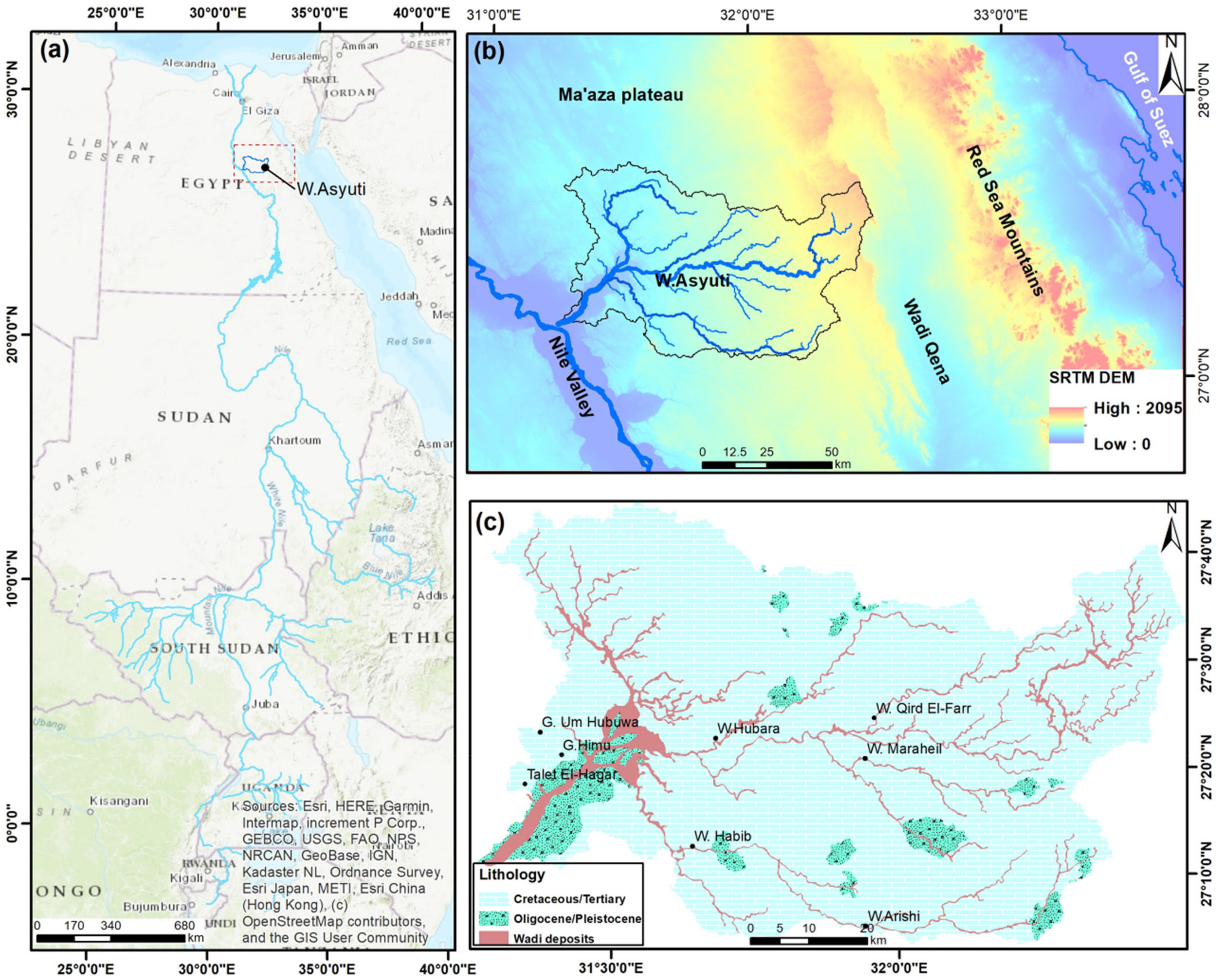
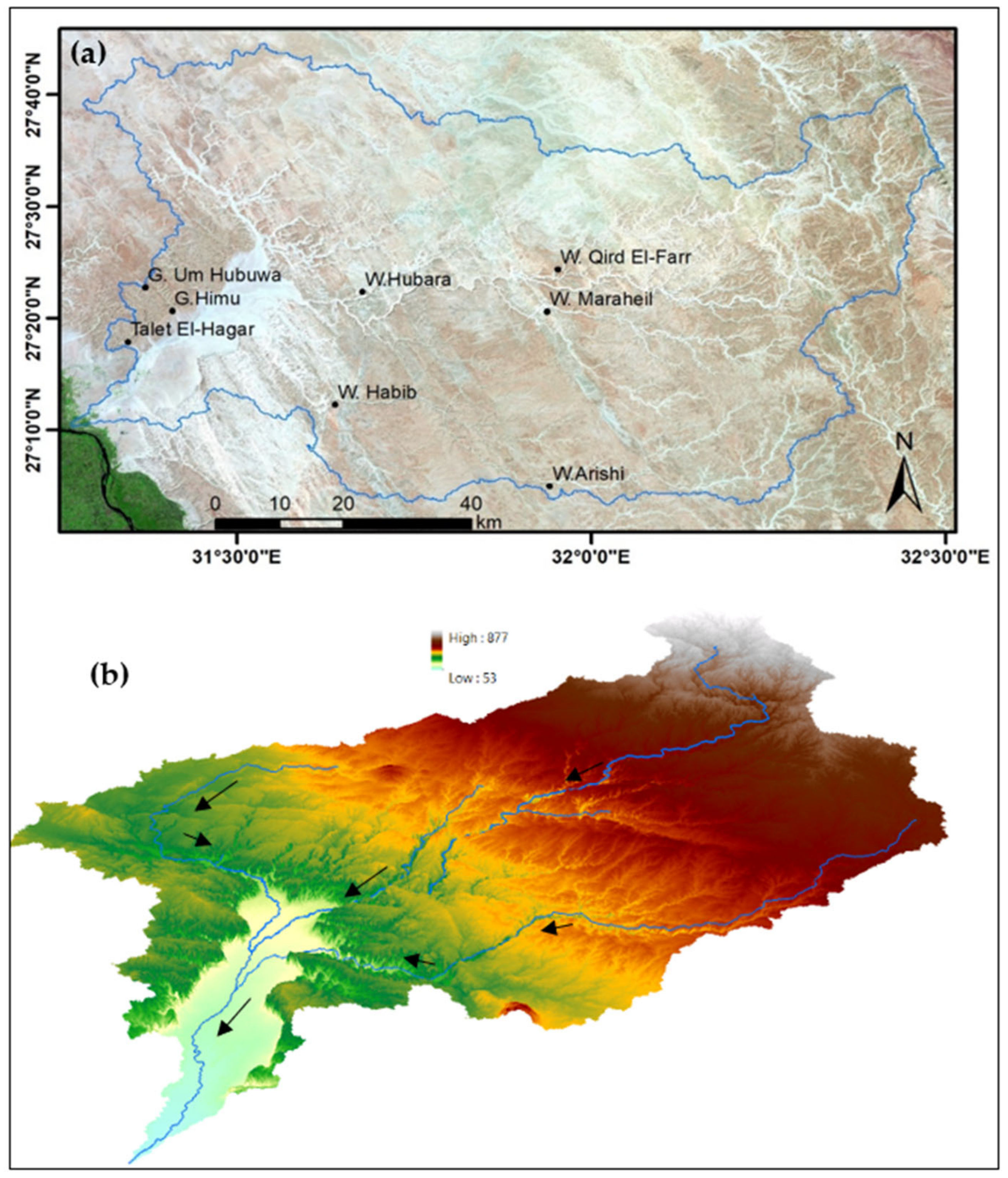
2. Study Area
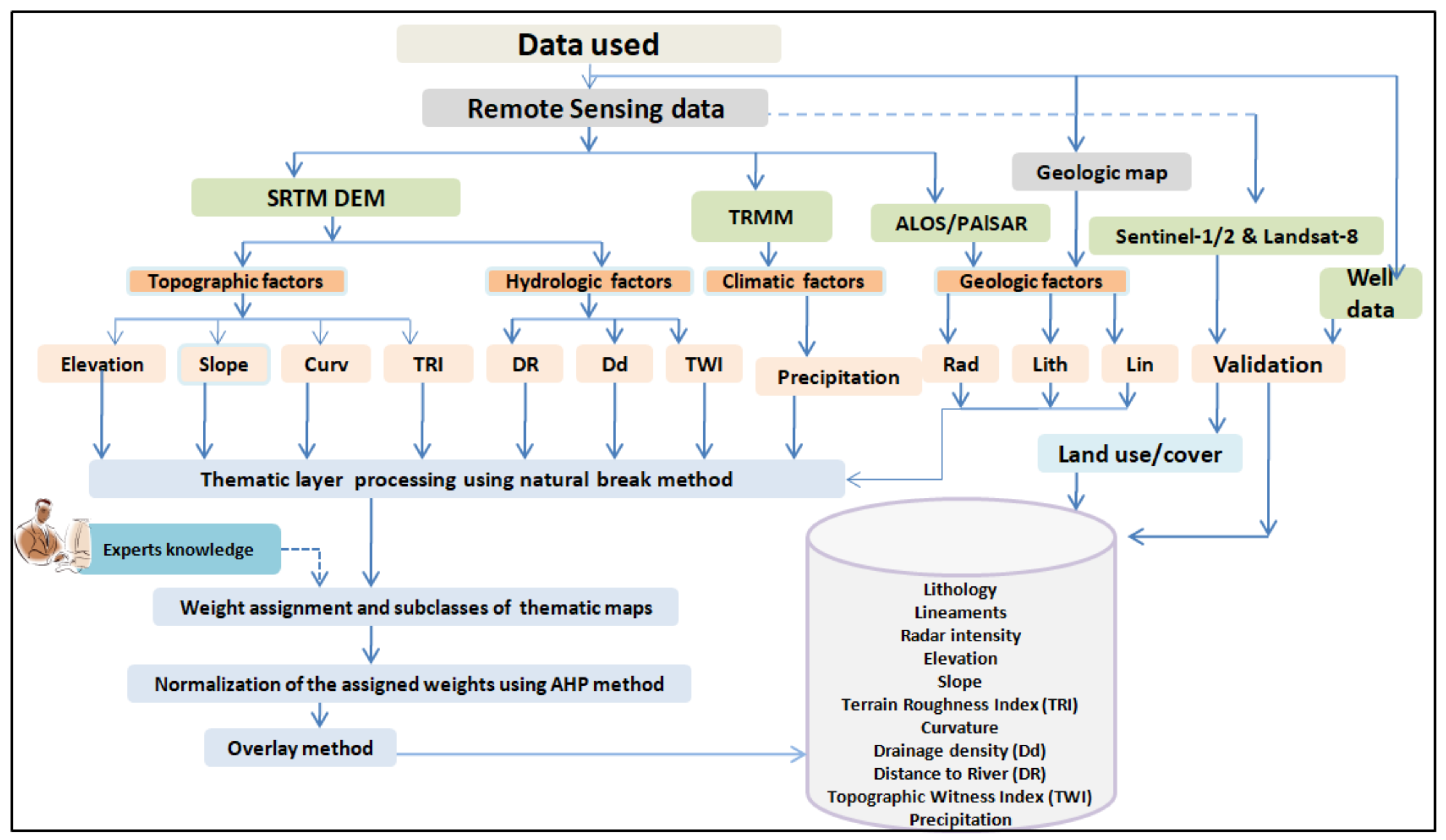
3. Data and Methods
4. Results
4.1. Geological Conditioning Factors
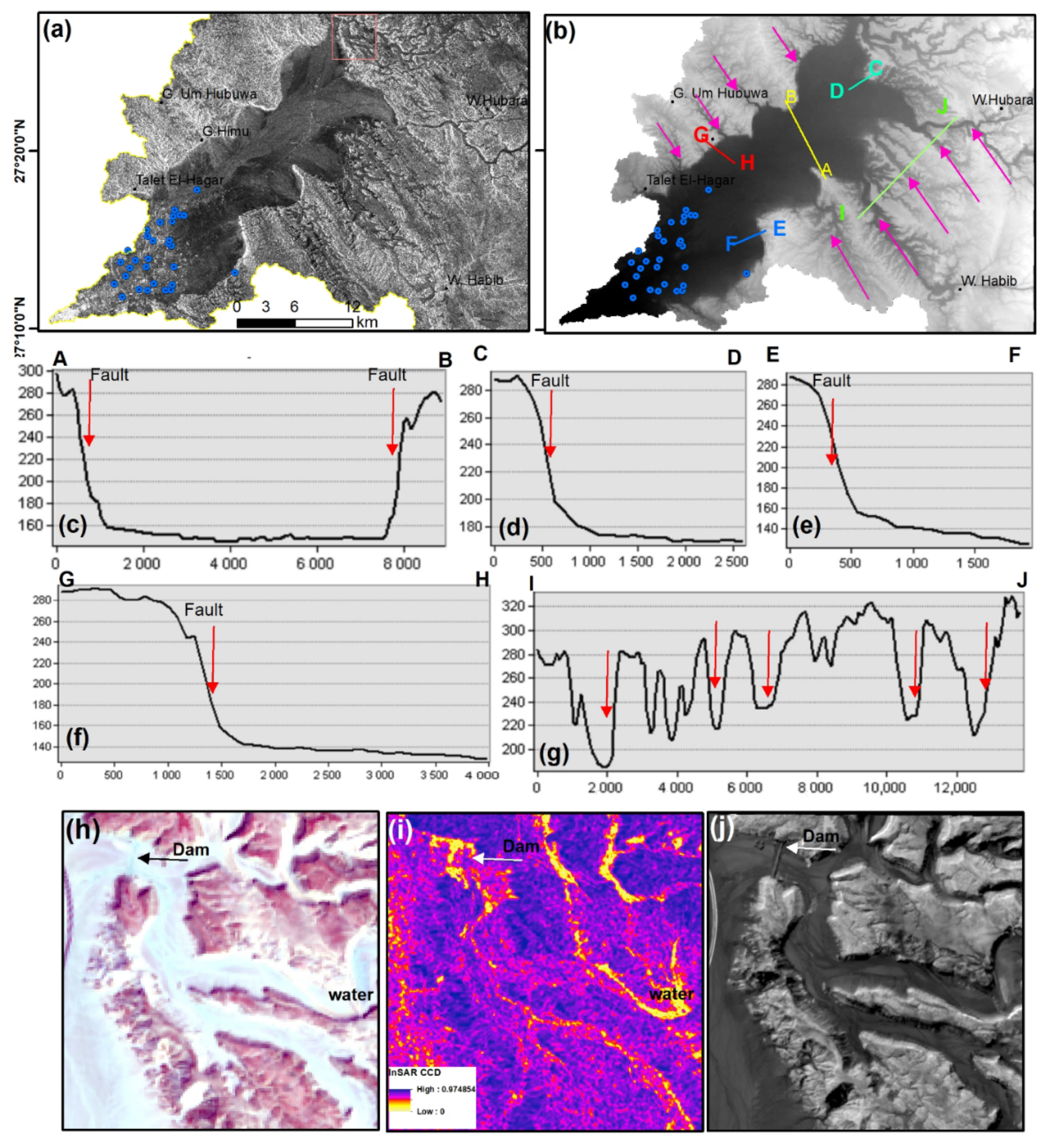
4.1.1. Geology/Geomorphology
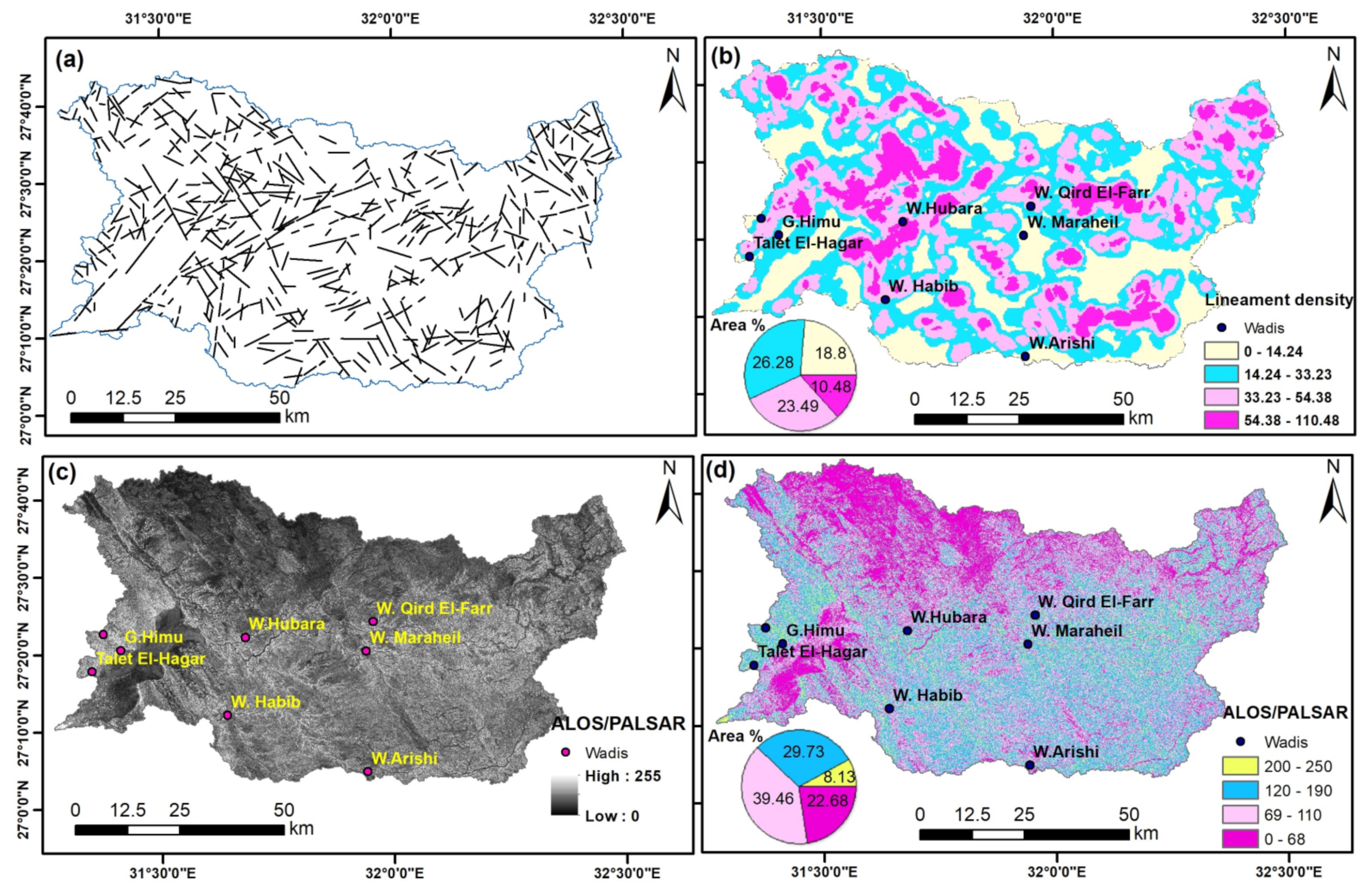
4.1.2. Lineaments
4.1.3. Radar Intensity
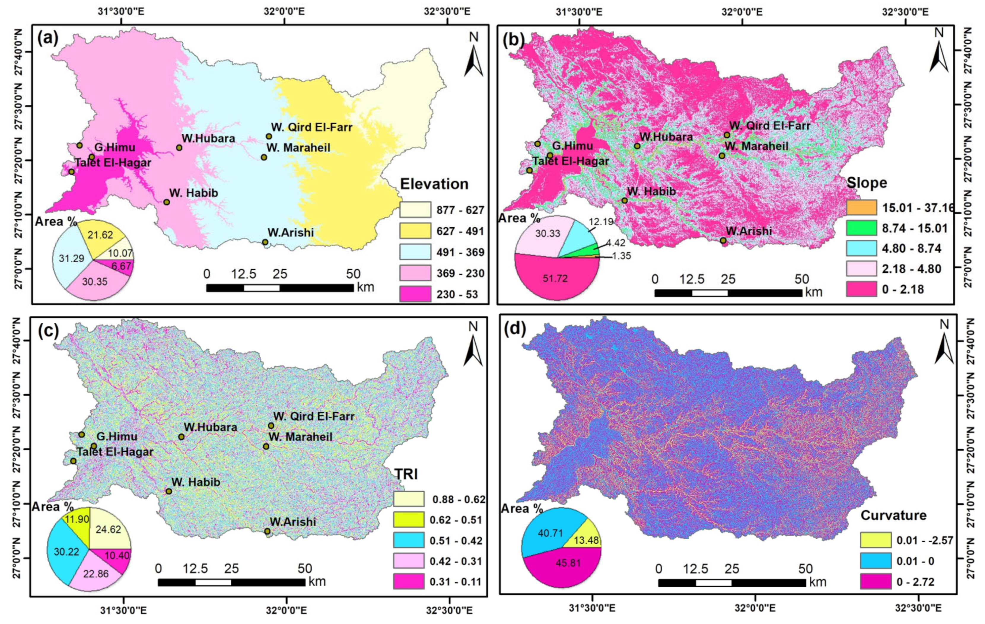
4.2. Topographical Conditioning Factors
4.2.1. Elevation
4.2.2. Slope
4.2.3. Roughness
4.2.4. Curvature
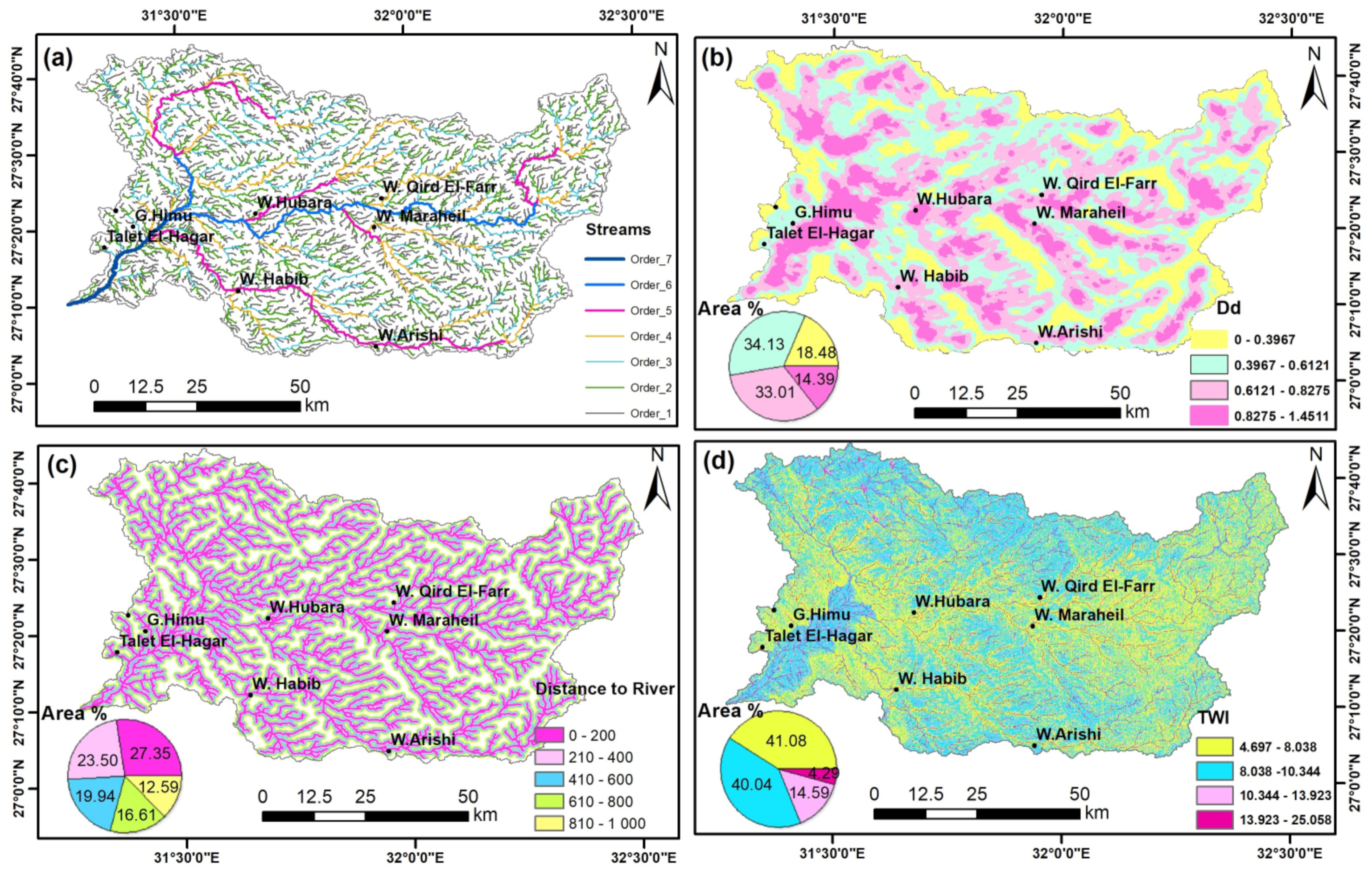
4.3. Hydrological Factors
4.3.1. Drainage Density (Dd)
4.3.2. Distance to River (DR)
4.3.3. TWI
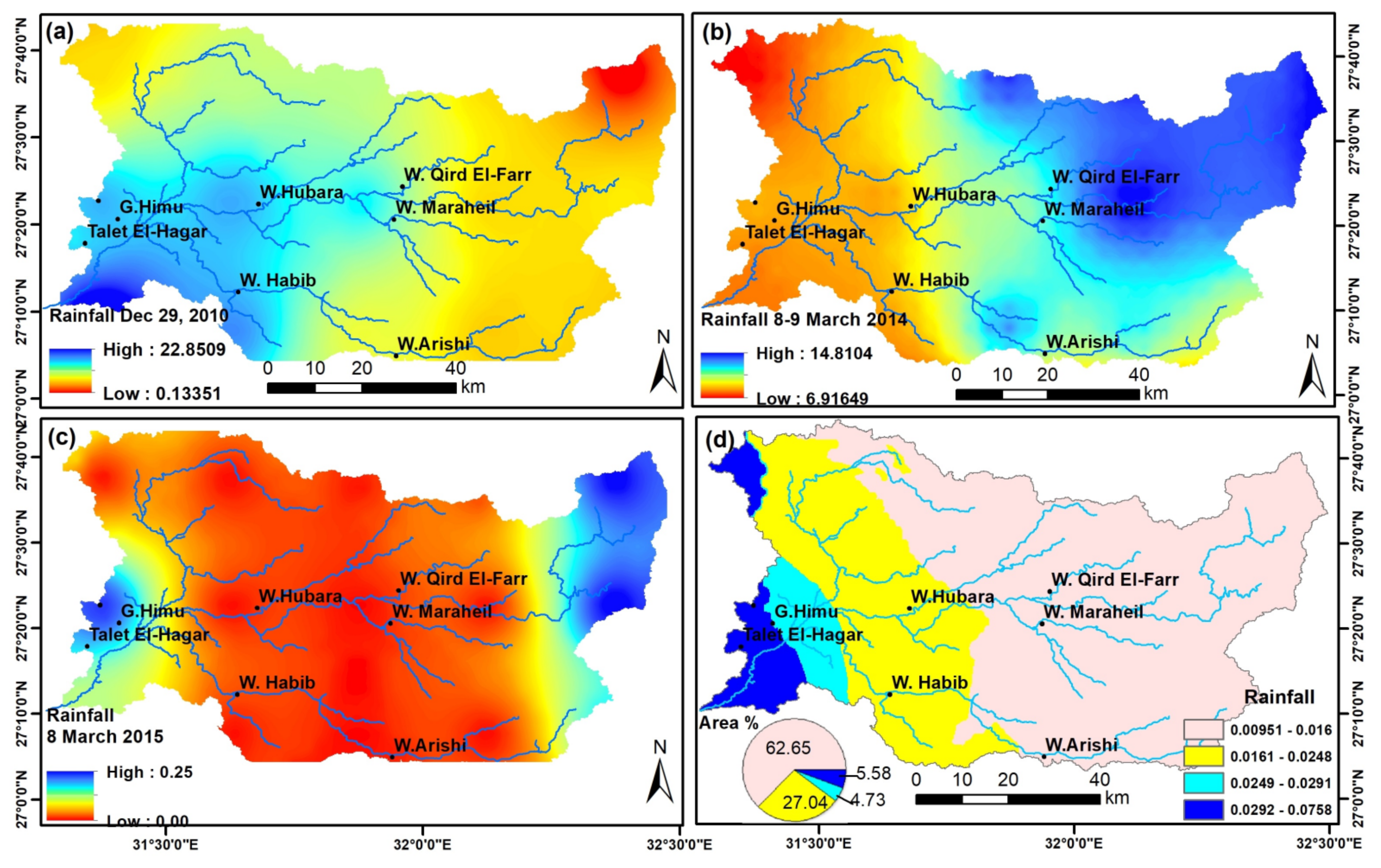
4.3.4. Rainfall Data
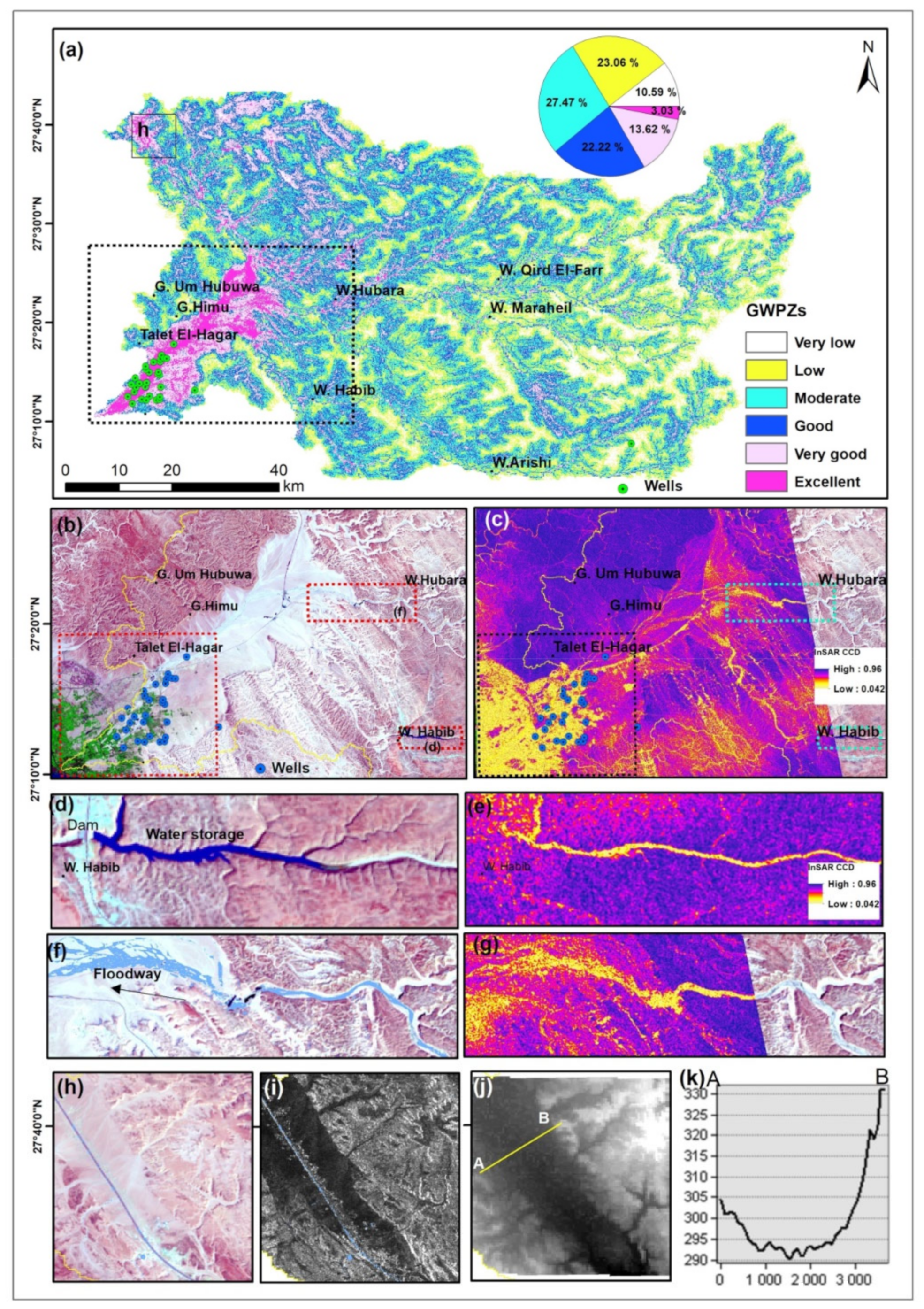
5. Prospective Groundwater Zones
6. Implications for the Detection of Changes in Land Use/Cover
7. Discussion
8. Conclusions
Author Contributions
Funding
Institutional Review Board Statement
Informed Consent Statement
Acknowledgments
Conflicts of Interest
Abbreviations
| SRTM | Shuttle Radar Topography Mission | DEM | Digital Elevation Model |
| TRMM | Tropical Rainfall Measuring Mission | OLI | Operational Land Imager |
| ALOS | Advanced Land Observing Satellite | RS | Remote Sensing |
| PALSAR | Phased-Array-Type L-band Synthetic Aperture Radar | AHP | Analytical Hierarchy Process |
| GIS | Geographic Information System | LU/LC | land use/land cover |
| TWI | Topographic Wetness Index | NIR | Near Infrared |
| GWPZs | Groundwater Prospective Zones | TIRS | Thermal Infrared Sensor |
| InSAR | Interferometry Synthetic Aperture Radar | CCD | Coherence Change Detection |
| NDVI | Normalized Difference Vegetation Index | MHz | Megahertz |
| 8D | Deterministic eight-neighbors | CR | Consistency ratio |
| USGS | United States Geological Survey | CI | Consistency Index |
| TRI | Terrain Roughness Index | SLC | single look complex |
| ENVI | Environment for Visualizing Images | R | Red band |
| WGS 84 | World Geodetic System 1984 | DR | Distance to river |
| Dd | Drainage density | Lin | Lineaments |
| Lith | Lithology | Rad | Radar intensity |
| Curv | Curvature | GW | Groundwater |
References
- Ranjan, S.P.; Kazama, S.; Sawamoto, M. Effects of climate and land use changes on groundwater resources in coastal aquifers. J. Environ. Manag. 2006, 80, 25–35. [Google Scholar] [CrossRef] [PubMed] [Green Version]
- Okello, C.; Tomasello, B.; Greggio, N.; Wambiji N and Antonellini, M. Impact of Population Growth and Climate Change on the Freshwater Resources of Lamu Island, Kenya. Water 2015, 7, 1264–1290. [Google Scholar] [CrossRef]
- Das, S. Comparison among influencing factor, frequency ratio, and analytical hierarchy process techniques for groundwater potential zonation in Vaitarna basin, Maharashtra, India. Groundw. Sustain. Dev. 2019, 8, 617–629. [Google Scholar] [CrossRef]
- Ramachandra, T.V. Soil and Groundwater Pollution from Agricultural Activities; Commonwealth of Learning: Vancouver, BC, Canada; Center for Ecological Science, Indian Institute of Science: Karnataka, India, 2006; p. 352. [Google Scholar]
- Mallick, J.; Khan, R.A.; Ahmed, M.; Alqadhi, S.D.; Alsubih, M.; Falqi, I.; Hasan, M.A. Modeling Groundwater Potential Zone in a Semi-Arid Region of Aseer Using Fuzzy-AHP and Geoinformation Techniques. Water 2019, 11, 2656. [Google Scholar] [CrossRef] [Green Version]
- Jha, M.K.; Bongane, G.M.; Chowdary, V.M. Groundwater potential zoning by remote sensing, GIS and MCDM techniques: A case study of eastern India. In Proceedings of the Symposium JS.4 at the IAHS and IAH convention, Hyderabad, India, 6–12 September 2009; IAHS Press: Wallingford, UK, 2009; pp. 432–441. [Google Scholar]
- Oh, H.-J.; Kim, Y.-S.; Choi, J.-K.; Park, E.; Lee, S. GIS mapping of regional probabilistic groundwater potential in the area of Pohang City, Korea. J. Hydrol. 2011, 399, 158–172. [Google Scholar] [CrossRef]
- Arkoprovo, B.; Adarsa, J.; ShashiPrakash, S. Delineation of groundwater potential zones using satellite remote sensing and geographic information techniques: A case study from Ganjam district, Orissa, India. Res. J. Recent Sci. 2012, 9, 59–66. [Google Scholar]
- Manap, M.A.; Sulaiman, W.N.A.; Ramli, M.F.; Pradhan, B.; Surip, N. A knowledge-driven GIS modeling technique for groundwater potential mapping at the Upper Langat Basin, Malaysia. Arab. J. Geosci. 2011, 6, 1621–1637. [Google Scholar] [CrossRef]
- UNESCO. The UN World Water Development Report. 2003. Available online: http://www.unesco.org/ (accessed on 1 January 2022).
- Park, S.; Hamm, S.-Y.; Jeon, H.-T.; Kim, J. Evaluation of Logistic Regression and Multivariate Adaptive Regression Spline Models for Groundwater Potential Mapping Using R and GIS. Sustainability 2017, 9, 1157. [Google Scholar] [CrossRef] [Green Version]
- El-Baz, F. Sand accumulation and groundwater in the eastern Sahara. Episodes 1998, 21, 147–151. [Google Scholar] [CrossRef]
- Abdelkareem, M.; Al-Arifi, N. The use of remotely sensed data to reveal geologic, structural, and hydrologic features and predict potential areas of water resources in arid regions. Arab. J. Geosci. 2021, 14, 1–15. [Google Scholar] [CrossRef]
- Avand, M.; Janizadeh, S.; Tien Bui, D.; Pham, V.H.; Ngo, P.T.T.; Nhu, V.-H. A tree-based intelligence ensemble approach for spatial prediction of potential groundwater. Int. J. Digit. Earth 2020, 13, 1408–1429. [Google Scholar] [CrossRef]
- Abdelkareem, M.; Abdalla, F. Revealing potential areas of water resources using integrated remote-sensing data and GIS-based analytical hierarchy process. Geocarto Int. 2021, 1–25. [Google Scholar] [CrossRef]
- Zhu, Q.; Abdelkareem, M. Mapping Groundwater Potential Zones Using a Knowledge-Driven Approach and GIS Analysis. Water 2021, 13, 579. [Google Scholar] [CrossRef]
- Singh, C.K.; Shashtri, S.; Singh, A.; Mukherjee, S. Quantitative modeling of groundwater in Satluj River basin of Rupnagar district of Punjab using remote sensing and geographic information system. Environ. Earth Sci. 2010, 62, 871–881. [Google Scholar] [CrossRef]
- Adiat, K.; Nawawi, M.; Abdullah, K. Assessing the accuracy of GIS-based elementary multi criteria decision analysis as a spatial prediction tool—A case of predicting potential zones of sustainable groundwater resources. J. Hydrol. 2012, 440–441, 75–89. [Google Scholar] [CrossRef]
- Abdelkareem, M.; El-Baz, F. Analyses of optical images and radar data reveal structural features and predict groundwater accumulations in the central Eastern Desert of Egypt. Arab. J. Geosci. 2014, 8, 2653–2666. [Google Scholar] [CrossRef]
- Jha, M.K.; Chowdhury, A.; Chowdary, V.M.; Peiffer, S. roundwater management and development by integrated remote sensing and geographic information systems: Prospects and constraints. Water Resour. Manag. 2007, 21, 427–467. [Google Scholar] [CrossRef]
- Rahman, A. A GIS based DRASTIC model for assessing groundwater vulnerability in shallow aquifer in Aligarh, India. Appl. Geogr. 2008, 28, 32–53. [Google Scholar] [CrossRef]
- Mondal, N.C.; Adike, S.; Singh, V.S.; Ahmed, S.; Jayakumar, K.V. Determining shallow aquifer vulnerability by the DRASTIC model and hydrochemistry in granitic terrain, southern India. J. Earth Syst. Sci. 2017, 126, 89. [Google Scholar] [CrossRef]
- Mondal, N.C.; Adike, S.; Ahmed, S. Development of entropy-based model for pollution risk assessment of hydrogeological system. Arab. J. Geosci. 2018, 11, 1–15. [Google Scholar] [CrossRef]
- Goswami, T.; Ghosa, S. Understanding the suitability of two MCDM techniques in mapping the groundwater potential zones of semi-arid Bankura District in eastern India. Groundw. Sustain. Dev. 2022, 17, 100727. [Google Scholar] [CrossRef]
- Aykut, T. Determination of groundwater potential zones using Geographical Information Systems (GIS) and Analytic Hierarchy Process (AHP) between Edirne-Kalkansogut (northwestern Turkey). Groundw. Sustain. Dev. 2021, 12, 100545. [Google Scholar] [CrossRef]
- Abdelkareem, M.; El-Baz, F.; Askalany, M.; Akawy, A.; Ghoneim, E. Groundwater prospect map of Egypt’s Qena Valley using data fusion. Int. J. Image Data Fusion 2012, 3, 169–189. [Google Scholar] [CrossRef]
- Satapathy, I.; Syed, T.H. Characterization of groundwater potential and artificial recharge sites in Bokaro District, Jharkhand (India), using remote sensing and GIS-based techniques. Environ. Earth Sci. 2015, 74, 4215–4232. [Google Scholar] [CrossRef]
- Machiwal, D.; Rangi, N.; Sharma, A. Integrated knowledge- and data-driven approaches for groundwater potential zoning using GIS and multi-criteria decision making techniques on hard-rock terrain of Ahar catchment, Rajasthan, India. Environ. Earth Sci. 2014, 73, 1871–1892. [Google Scholar] [CrossRef]
- Rahmati, O.; Samani, A.N.; Mahdavi, M.; Pourghasemi, H.R.; Zeinivand, H. Groundwater potential mapping at Kurdistan region of Iran using analytic hierarchy process and GIS. Arab. J. Geosci. 2014, 8, 7059–7071. [Google Scholar] [CrossRef]
- Razandi, Y.; Pourghasemi, H.R.; Neisani, N.S.; Rahmati, O. Application of analytical hierarchy process, frequency ratio, and certainty factor models for groundwater potential mapping using GIS. Earth Sci. Informatics 2015, 8, 867–883. [Google Scholar] [CrossRef]
- Kumar, V.A.; Mondal, N.C.; Ahmed, S. Identification of Groundwater Potential Zones Using RS, GIS and AHP Techniques: A Case Study in a Part of Deccan Volcanic Province (DVP), Maharashtra, India. J. Indian Soc. Remote Sens. 2020, 48, 497–511. [Google Scholar] [CrossRef]
- Riad, P.; Billib, M.; Hassan, A.; Salam, M.A.; El Din, M.N. Application of the overlay weighted model and boolean logic to determine the best locations for artificial recharge of groundwater. J. Urban Environ. Eng. 2011, 5, 57–66. [Google Scholar] [CrossRef]
- Muthumaniraja, C.K.; Anbazhagan, S.; Jothibasu, A.; Chinnamuthu, M. Remote sensing and fuzzy logic approach for artificial recharge studies in hard rock terrain of South India. In GIS and Geostatistical Techniques for Groundwater Science; Elsevier: Amsterdam, The Netherlands, 2019; pp. 91–112. [Google Scholar]
- Balamurugan, G.; Seshan, K.; Bera, S. Frequency ratio model for groundwater potential mapping and its sustainable management in cold desert, India. J. King Saud Univ. Sci. 2017, 29, 333–347. [Google Scholar]
- Naghibi, S.A.; Pourghasemi, H.R.; Pourtaghi, Z.S.; Rezaei, A. Groundwater qanat potential mapping using frequency ratio and Shannon’s entropy models in the Moghan watershed, Iran. Earth Sci. Informatics 2015, 8, 171–186. [Google Scholar] [CrossRef]
- Yariyan, P.; Avand, M.; Omidvar, E.; Pham, Q.B.; Linh, N.T.T.; Tiefenbacher, J.P. Optimization of statistical and machine learning hybrid models for groundwater potential mapping. Geocarto Int. 2020, 11, 2282–2314. [Google Scholar] [CrossRef]
- Ozdemir, A. GIS-based groundwater spring potential mapping in the Sultan Mountains (Konya, Turkey) using frequency ratio, weights of evidence and logistic regression methods and their comparison. J. Hydrol. 2011, 411, 290–308. [Google Scholar] [CrossRef]
- Chen, W.; Li, H.; Hou, E.; Wang, S.; Wang, G.; Panahi, M.; Li, T.; Peng, T.; Guo, C.; Niu, C.; et al. GIS-based groundwater potential analysis using novel ensemble weights-of-evidence with logistic regression and functional tree models. Sci. Total Environ. 2018, 634, 853–867. [Google Scholar] [CrossRef] [Green Version]
- Corsini, A.; Cervi, F.; Ronchetti, F. Weight of evidence and artificial neural networks for potential groundwater mapping: An application to the Mt. Modino area (Northern Apennines, Italy). Geomorphology 2009, 111, 79–87. [Google Scholar] [CrossRef]
- Mogaji, K.A.; Omosuyi, G.O.; Adelusi, A.O.; Lim, H.S. Application of GIS-Based Evidential Belief Function Model to Regional Groundwater Recharge Potential Zones Mapping in Hardrock Geologic Terrain. Environ. Process. 2016, 3, 93–123. [Google Scholar] [CrossRef]
- Lee, S.; Hong, S.-M.; Jung, H.-S. GIS-based groundwater potential mapping using artificial neural network and support vector machine models: The case of Boryeong city in Korea. Geocarto Int. 2017, 33, 847–861. [Google Scholar] [CrossRef]
- Saaty, T. A scaling method for priorities in hierarchical structures. J. Math. Psychology. 1977, 15, 234–281. [Google Scholar] [CrossRef]
- Saaty, T.L. The Analytic Hierarchy Process: Planning, Priority Setting, Resource Allocation; McGraw-Hill: New York, NY, USA, 1980. [Google Scholar]
- Melese, T.; Belay, T. Groundwater Potential Zone Mapping Using Analytical Hierarchy Process and GIS in Muga Watershed, Abay Basin, Ethiopia. Glob. Chall. 2021, 6, 2100068. [Google Scholar] [CrossRef]
- Ghosh, A.; Adhikary, P.P.; Bera, B.; Bhunia, G.S.; Shit, P.K. Assessment of groundwater potential zone using MCDA and AHP techniques: Case study from a tropical river basin of India. Appl. Water Sci. 2022, 12, 37. [Google Scholar] [CrossRef]
- Ifediegwu, S.I. Assessment of groundwater potential zones using GIS and AHP techniques: A case study of the Lafia district, Nasarawa State, Nigeria. Appl. Water Sci. 2022, 12, 10. [Google Scholar] [CrossRef]
- Yin, H.; Shi, Y.; Niu, H.; Xie, D.; Wei, J.; Lefticariu, L.; Xu, S. A GIS-based model of potential groundwater yield zonation for a sandstone aquifer in the Juye Coalfield, Shangdong, China. J. Hydrol. 2017, 557, 434–447. [Google Scholar] [CrossRef]
- Arulbalaji, P.; Padmalal, D.; Sreelash, K. GIs and AHP techniques Based Delineation of Groundwater Potential Zones: A case study from southern Western Ghats, India. Sci. Rep. 2019, 9, 2082. [Google Scholar] [CrossRef]
- Lettenmaier, D.P.; Alsdorf, D.; Dozier, J.; Huffman, G.J.; Pan, M.; Wood, E.F. In roads of remote sensing into hydrologic science during the WRR era. Water Resour Res. 2015, 51, 7309–7342. [Google Scholar] [CrossRef]
- Murmu, P.; Kumar, M.; Lal, D.; Sonker, I.; Singh, S.K. Delineation of groundwater potential zones using geospatial techniques and analytical hierarchy process in Dumka district, Jharkhand, India. Groundw. Sustain. Dev. 2019, 9, 100239. [Google Scholar] [CrossRef]
- Sahu, U.; Wagh, V.; Mukate, S.; Kadam, A.; Patil, S. Applications of geospatial analysis and analytical hierarchy process to identify the groundwater recharge potential zones and suitable recharge structures in the Ajani-Jhiri watershed of north Maharashtra, India. Groundw. Sustain. Dev. 2022, 17, 100733. [Google Scholar] [CrossRef]
- Priya, U.; Iqbal, M.A.; Abdus Salam, M.; Nur-E-Alam, M.; Uddin, M.F.; Islam, A.T.; Sarkar, S.K.; Imran, S.I.; Eh Rak, A. Sustainable Groundwater Potential Zoning with Integrating GIS, Remote Sensing, and AHP Model: A Case from North-Central Bangladesh. Sustainability 2022, 14, 5640. [Google Scholar] [CrossRef]
- Castillo, J.L.U.; Martínez Cruz, D.A.; Ramos Leal, J.A.; Tuxpan Vargas, J.; Rodríguez Tapia, S.A.; Marín Celestino, A.E. Delineation of Groundwater Potential Zones (GWPZs) in a Semi-Arid Basin through Remote Sensing, GIS, and AHP Approaches. Water 2022, 14, 2138. [Google Scholar] [CrossRef]
- Maity, B.; Mallick, S.K.; Das, P.; Rudra, S. Comparative analysis of groundwater potentiality zone using fuzzy AHP, frequency ratio and Bayesian weights of evidence methods. Applied Water Science 2022, 12, 63. [Google Scholar] [CrossRef]
- Grohmann, C.H.; Riccomini, C.; Alves, F.M. SRTM-based morphotectonic analysis of the Pocos de Caldas Alkaline Massif, Southeastern Brazil. Comput. Geosci. 2007, 33, 10–19. [Google Scholar] [CrossRef] [Green Version]
- Mallupatt, P.K.; Redd, J.R.S. Analysis of Land Use/Land Cover Changes Using Remote Sensing Data and GIS at an Urban Area, Tirupati, India. Sci. World J. 2013, 2013, 268623. [Google Scholar] [CrossRef] [Green Version]
- Mas, J.F. Monitoring land-cover changes: A comparison of change detection techniques. Int. J. Remote Sens. 1999, 20, 139–152. [Google Scholar] [CrossRef]
- Conoco. Geological map of Egypt, Scale 1:500,000; The Egyptian General Petroleum Corporation: Cairo, Egypt, 1987. [Google Scholar]
- Youssef, M.M.; Riad, S.; Mansour, H.H. Surface and subsurface structural study of the Area around Assiut, Egypt. Bull. Fac. Sci. Assiut. Univ. 1977, 6, 293–306. [Google Scholar]
- O’Callaghan, J.F.; Mark, D.M. The extraction of drainage networks from digital elevation data. Comput. Vis. Graph. Image Process. 1984, 28, 323–344. [Google Scholar] [CrossRef]
- Havivi, S.; Amir, D.; Schvartzman, I.; August, Y.; Maman, S.; Rotman, S.R.; Blumberg, D.G. Mapping dune dynamics by InSAR coherence. Earth Surf. Process. Landforms 2018, 43, 1229–1240. [Google Scholar] [CrossRef]
- Ullmann, T.; Büdel, C.; Baumhauer, P.; Padashi, M. Sentinel-1 SAR Data Revealing Fluvial Morphodynamics in Damghan (Iran): Amplitude and Coherence Change Detection. Int. J. Earth Sci. Geophys. 2016, 2, 7. [Google Scholar]
- Ayazi, M.H.; Pirasteh, S.; Arvin, A.K.P.; Pradhan, B.; Nikouravan, B.; Mansor, S. Disasters and risk reduction in groundwater: Zagros mountain southwest Iran using geo-informatics techniques. Dis. Adv. 2010, 3, 51–57. [Google Scholar]
- Selvarani, A.G.; Maheswaran, G.; Elangovan, K. Identification of Artificial Recharge Sites for Noyyal River Basin Using GIS and Remote Sensing. J. Indian Soc. Remote Sens. 2017, 45, 67–77. [Google Scholar] [CrossRef]
- Achu, A.L.; Reghunath, R.; Thomas, J. Mapping of Groundwater Recharge Potential Zones and Identification of Suitable Site-Specific Recharge Mechanisms in a Tropical River Basin. J. Earth Syst. Environ. 2020, 4, 131–145. [Google Scholar] [CrossRef]
- Pradhan, A.M.S.; Kim, Y.T. Relative e_ect method of landslide susceptibility zonation in weathered granite soil: A case study in Deokjeok-ri Creek, South Korea. Nat. Hazards 2014, 72, 1189–1217. [Google Scholar] [CrossRef]
- Pradhan, B.; Youssef, A.M. Manifestation of remote sensing data and GIS for landslide hazard analysis using spatial-based statistical models. Arab. J. Geosci. 2009, 3, 319–326. [Google Scholar] [CrossRef]
- Pradhan, B. Groundwater potential zonation for basaltic watersheds using satellite remote sensing data and GIS techniques. Cent. Eur. J. Geosci. 2009, 1, 120–129. [Google Scholar] [CrossRef]
- Abdekareem, M.; Al-Arifi, N.; Abdalla, F.; Mansour, A.; El-Baz, F. Fusion of Remote Sensing Data Using GIS-Based AHP-Weighted Overlay Techniques for Groundwater Sustainability in Arid Regions. Sustainability 2022, 14, 7871. [Google Scholar] [CrossRef]
- Hung, L.Q.; Batelaan, O.; de Smedt, F. Lineament extraction and analysis, comparison of LANDSAT ETM and ASTER imagery. Case study: Suoimuoi tropical karst catchment, Vietnam. Proc. SPIE 2005, 5983, 59830T–59831T. [Google Scholar] [CrossRef]
- Assatse, W.T.; Nouck, P.N.; Tabod, C.T.; Akame, J.M.; Biringanine, G.N. Hydrogeological activity of lineaments in Yaoundé Cameroon region using remote sensing and GIS techniques. Egypt J. Remote Sens. Space Sci. 2016, 19, 49–60. [Google Scholar] [CrossRef] [Green Version]
- Jensen, J.R. Remote Sensing of the Environment: An Earth Resource Perspective; Prentice-Hall: Englewood Cliffs, UK, 2000; p. 544. [Google Scholar]
- Al Saud, M. Mapping potential areas for groundwater storage in wadiaurnah basin, western Arabian peninsula, using remote sensing and geographic information system techniques. Hydrogeol. J. 2010, 18, 1481–1495. [Google Scholar] [CrossRef]
- Ettazarini, S. Groundwater potential index: A strategically conceived tool for water research in fractured aquifers. Environ Geol. 2007, 52, 477–487. [Google Scholar] [CrossRef]
- Mukherjee, I.; Singh, U.K. Delineation of groundwater potential zones in a drought-prone semi-arid region of east India using GIS and analytical hierarchical process techniques. CATENA 2020, 194, 104681. [Google Scholar] [CrossRef]
- Yeh, H.-F.; Lee, C.-H.; Hsu, K.-C.; Chang, P.-H. GIS for the assessment of the groundwater recharge potential zone. Environ. Geol. 2009, 58, 185–195. [Google Scholar] [CrossRef]
- Yeh, H.-F.; Cheng, Y.-S.; Lin, H.-I.; Lee, C.-H. Mapping groundwater recharge potential zone using a GIS approach in Hualian River, Taiwan. Sustain. Environ. Res. 2016, 26, 33–43. [Google Scholar] [CrossRef] [Green Version]
- Kalantar, B.; Al-Najjar, H.A.H.; Pradhan, B.; Saeidi, V.; Halin, A.A.; Ueda, N.; Naghibi, S.A. Optimized Conditioning Factors Using Machine Learning Techniques for Groundwater Potential Mapping. Water 2019, 11, 1909. [Google Scholar] [CrossRef] [Green Version]
- Moghaddam, D.D.; Rahmati, O.; Haghizadeh, A.; Kalantari, Z. A Modeling Comparison of Groundwater Potential Mapping in a Mountain Bedrock Aquifer: QUEST, GARP, and RF Models. Water 2020, 12, 679. [Google Scholar] [CrossRef] [Green Version]
- Benjmel, K.; Amraoui, F.; Boutaleb, S.; Ouchchen, M.; Tahiri, A.; Touab, A. Mapping of Groundwater Potential Zones in Crystalline Terrain Using Remote Sensing, GIS Techniques, and Multicriteria Data Analysis (Case of the Ighrem Region, Western Anti-Atlas, Morocco). Water 2020, 12, 471. [Google Scholar] [CrossRef] [Green Version]
- Harini, P.; Sahadevan, D.K.; Das, I.C.; Manikyamba, C.; Durgaprasad, M.; Nandan, M.J. Regional groundwater assessment of Krishna RiverBasin using integrated GISapproach. J. Indian Soc. Remote Sens. 2018, 46, 1365–1377. [Google Scholar] [CrossRef]
- Dinesh Kumar, P.K.; Gopinath, G.; Seralathan, P. Application ofremote sensing and GIS for the demarcation of groundwater potential zones of a river basin inKerala, southwest cost of India. Int. J. Remote Sens. 2007, 28, 5583–5601. [Google Scholar] [CrossRef]
- Magesh, N.S.; Chandrasekar, N.; Soundranayagam, J.P. Delineation of groundwater potential zones in Theni district, Tamil Nadu, using remote sensing, GIS and MIF techniques. Geosci. Front. 2012, 3, 189–196. [Google Scholar] [CrossRef] [Green Version]
- Cevik, E.; Topal, T. GIS-based landslide susceptibility mapping for aproblematic segment of the natural pipeline, Hendek (Turkey). Environ. Geol. 2003, 44, 949–962. [Google Scholar] [CrossRef]
- Pinto, D.; Shrestha, S.; Babel, M.S.; Ninsawat, S. Delineation of groundwater potential zones in the Comoro watershed, Timor Leste using GIS, remote sensing and analytichierarchy process (AHP) technique. Appl. Water Sci. 2017, 7, 503–519. [Google Scholar] [CrossRef] [Green Version]
- Pande, C.B.; Khadri, S.F.R.; Moharir, K.N.; Patode, R.S. Assessment of groundwater potential zonation of Mahesh River basin Akola and Buldhana districts, Maharashtra, India using remote sensing and GIS techniques. Sustain. Water Resour. Manag. 2017, 4, 965–979. [Google Scholar] [CrossRef]
- Lentswe, G.B.; Lentswe, M. Delineation of potential groundwater recharge zones using analytic hierarchy process-guided GIS in the semi-arid Motloutse watershed, eastern Botswana. J. Hydrol. Reg. Stud. 2020, 28, 100674. [Google Scholar] [CrossRef]
- Hong, Y.; Abdelkareem, M. Integration of remote sensing and a GIS-based method for revealing prone areas to flood hazards and predicting optimum areas of groundwater resources. Arab. J. Geosci. 2022, 15, 1–14. [Google Scholar] [CrossRef]
- Villeneuve, S.; Cook, P.G.; Shanafield, M.; Wood, C.; White, N. Groundwater recharge via infiltration through an ephemeral riverbed, central Australia. J. Arid. Environ. 2015, 117, 47–58. [Google Scholar] [CrossRef]
- Rahmati, O.; Melesse, A.M. Application of Dempster–Shafer theory, spatial analysis and remote sensing for groundwater potentiality and nitrate pollution analysis in the semi-arid region of Khuzestan, Iran. Sci. Total Environ. 2016, 568, 1110–1123. [Google Scholar] [CrossRef]
- Razavi-Termeh, S.V.; Sadeghi-Niaraki, A.; Choi, S.-M. Groundwater Potential Mapping Using an Integrated Ensemble of Three Bivariate Statistical Models with Random Forest and Logistic Model Tree Models. Water 2019, 11, 1596. [Google Scholar] [CrossRef] [Green Version]
- Moore, I.D.; Grayson, R.B.; Ladson, A.R. Digital terrain modelling: A review of hydrological, geomorphological, and biological applications. Hydrol. Process. 1991, 5, 3–30. [Google Scholar] [CrossRef]
- Kavitha, B.; Kumar, D.S. Trends and effects of rainfall on groundwater recharge in Namakkal district of Tamil Nadu: Analysis using the Mann–Kendall test and transfer function model. Agric. Econ. Res. Rev. 2020, 33, 119–126. [Google Scholar] [CrossRef]
- Souissi, D.; Msaddek, M.H.; Zouhri, L.; Chenini, I.; El May, M.; Dlala, M. Mapping groundwater recharge potential zones in arid region using GIS and Landsat approaches, southeast Tunisia. Hydrol. Sci. J. 2018, 63, 251–268. [Google Scholar] [CrossRef]
- Paillou, P.; Schuster, M.; Tooth, S.; Far, T.; Rosenqvist, A.; Lopez, S.; Malezieux, J. Mapping of a major paleodrainage system in eastern Libya using orbital imaging radar: The Kufrah River. Earth Planet Sci. Lett. 2009, 277, 327–333. [Google Scholar] [CrossRef]
- Haynes, C.V., Jr. The Clovis Culture. Can. J. Anthropol. 1980, 1, 115–121. [Google Scholar]
- Abdelkareem, M.; El-Baz, F. Mode of formation of the Nile Gorge in northern Egypt: A study by DEM-SRTM data and GIS analysis. Geol. J. 2015, 51, 760–778. [Google Scholar] [CrossRef]
- Gheith, H.; Sultan, M. Construction of a hydrologic model for estimating Wadi runoff and groundwater recharge in the Eastern Desert, Egypt. J. Hydrol. 2002, 263, 36–55. [Google Scholar] [CrossRef]
- Beven, K.J.; Kirkby, M.J. A physically based, variable contributing area model of basin hydrology/Un modele a base physique de zone d’appel variable de l’hydrologie du bassin versant. Hydrol. Sci. J. 1979, 24, 43–69. [Google Scholar] [CrossRef] [Green Version]
- Abdelkareem, M. Targeting flash flood potential areas using remotely sensed data and GIS techniques. Nat. Hazards 2016, 85, 19–37. [Google Scholar] [CrossRef]
- Ferretti, A.; Monti-Guarnieri, A.; Prati, C.; Rocca, F.; Massonet, D. InSAR Principles-Guidelines for SAR Interferometry Processing and Interpretation; ESA Publications: Noordwijk, The Netherlands, 2007. [Google Scholar]
- Gaber, A.; Abdelkareem, M.; Abdelsadek, I.S.; Koch, M.; El-Baz, F. Using InSAR Coherence for Investigating the Interplay of Fluvial and Aeolian Features in Arid Lands: Implications for Groundwater Potential in Egypt. Remote Sens. 2018, 10, 832. [Google Scholar] [CrossRef] [Green Version]


| No | Type of Data | Source | Date | Resolution |
|---|---|---|---|---|
| 1 | Landsat-8 OLI | USGS | 15 March 2014 26 September 2021 | bands 2, 3, 4, 5, 6, and 7 (30 m) |
| 2 | Landsat-5 TM | USGS | 29 September 1987 | bands 1, 2, 3, 4, 5, and 7 (30 m resolution) |
| 3 | Sentinel-1 | ESA/Copernicus | 19 February 2017 18 February 2015 | C-band SLC (12.5 m) |
| 4 | Sentinel-2 | ESA/Copernicus | 14 March 2022 20 March 2016 | bands 2, 3, 4, 8 (“10” m), 11, and 12 (“20” m) |
| 5 | PALSAR-2 Jaxa | Jaxa | 2017 | 25 m |
| 6 | SRTM DEM | USGS | 11–22 February 2000 | C-band (30 m) |
| 7 | TRMM data | NASA | 1 January 1998–1 November 2015 | 0.25 degrees in latitude and longitudes |
| Lith | Lin | Rad | Elev | Slope | TRI | Curv | Dd | D.R | TWI | Rainfall | |
|---|---|---|---|---|---|---|---|---|---|---|---|
| Lith | 1.00 | 1.33 | 1.14 | 1.60 | 1.33 | 1.60 | 2.00 | 1.33 | 1.00 | 1.14 | 1.60 |
| Lin | 0.75 | 1.00 | 0.86 | 1.20 | 1.00 | 1.20 | 1.50 | 1.00 | 0.75 | 0.86 | 1.20 |
| Rad | 0.88 | 1.17 | 1.00 | 1.40 | 1.17 | 1.40 | 1.75 | 1.17 | 0.88 | 1.00 | 1.40 |
| Elev | 0.63 | 0.83 | 0.71 | 1.00 | 0.83 | 1.00 | 1.25 | 0.83 | 0.63 | 0.71 | 1.00 |
| Slope | 0.75 | 1.00 | 0.86 | 1.20 | 1.00 | 1.20 | 1.50 | 1.00 | 0.75 | 0.86 | 1.20 |
| TRI | 0.63 | 0.83 | 0.71 | 1.00 | 0.83 | 1.00 | 1.25 | 0.83 | 0.63 | 0.71 | 1.00 |
| Curv | 0.50 | 0.67 | 0.57 | 0.80 | 0.67 | 0.80 | 1.00 | 0.67 | 0.50 | 0.57 | 0.80 |
| Dd | 0.75 | 1.00 | 0.86 | 1.20 | 1.00 | 1.20 | 1.50 | 1.00 | 0.75 | 0.86 | 1.20 |
| D R | 1.00 | 1.33 | 1.14 | 1.60 | 1.33 | 1.60 | 2.00 | 1.33 | 1.00 | 1.14 | 1.60 |
| TWI | 0.88 | 1.17 | 1.00 | 1.40 | 1.17 | 1.40 | 1.75 | 1.17 | 0.88 | 1.00 | 1.40 |
| Rainfall | 0.63 | 0.83 | 0.71 | 1.00 | 0.83 | 1.00 | 1.25 | 0.83 | 0.63 | 0.71 | 1.00 |
| Lith | Lin | Rad | Elev | Slope | TRI | Curv | Dd | D.R | TWI | Rainfall | Sum | λmax | |
|---|---|---|---|---|---|---|---|---|---|---|---|---|---|
| Lith | 0.119 | 0.119 | 0.119 | 0.119 | 0.119 | 0.119 | 0.119 | 0.119 | 0.119 | 0.119 | 0.119 | 1.313 | 11 |
| Lin | 0.090 | 0.090 | 0.090 | 0.090 | 0.090 | 0.090 | 0.090 | 0.090 | 0.090 | 0.090 | 0.090 | 0.985 | 11 |
| Rad | 0.104 | 0.104 | 0.104 | 0.104 | 0.104 | 0.104 | 0.104 | 0.104 | 0.104 | 0.104 | 0.104 | 1.149 | 11 |
| Elev | 0.075 | 0.075 | 0.075 | 0.075 | 0.075 | 0.075 | 0.075 | 0.075 | 0.075 | 0.075 | 0.075 | 0.821 | 11 |
| Slope | 0.090 | 0.090 | 0.090 | 0.090 | 0.090 | 0.090 | 0.090 | 0.090 | 0.090 | 0.090 | 0.090 | 0.985 | 11 |
| TRI | 0.075 | 0.075 | 0.075 | 0.075 | 0.075 | 0.075 | 0.075 | 0.075 | 0.075 | 0.075 | 0.075 | 0.821 | 11 |
| Curv | 0.060 | 0.060 | 0.060 | 0.060 | 0.060 | 0.060 | 0.060 | 0.060 | 0.060 | 0.060 | 0.060 | 0.657 | 11 |
| Dd | 0.090 | 0.090 | 0.090 | 0.090 | 0.090 | 0.090 | 0.090 | 0.090 | 0.090 | 0.090 | 0.090 | 0.985 | 11 |
| DR | 0.119 | 0.119 | 0.119 | 0.119 | 0.119 | 0.119 | 0.119 | 0.119 | 0.119 | 0.119 | 0.119 | 1.313 | 11 |
| TWI | 0.104 | 0.104 | 0.104 | 0.104 | 0.104 | 0.104 | 0.104 | 0.104 | 0.104 | 0.104 | 0.104 | 1.149 | 11 |
| Rainfall | 0.075 | 0.075 | 0.075 | 0.075 | 0.075 | 0.075 | 0.075 | 0.075 | 0.075 | 0.075 | 0.075 | 0.821 | 11 |
| Factor | Factor/Weight | Subclasses | Rank | Normalized Sub-Class | Area % |
|---|---|---|---|---|---|
| Geologic factors | Lithology (0.119) | Cretaceous/Tertiary | 1 | 0.077 | 86.81 |
| Oligocene/Plei stocene | 4 | 0.308 | 6.05 | ||
| Wadi deposits | 8 | 0.615 | 7.14 | ||
| Lineaments (0.090) | 0 to 14.24 | 1 | 0.063 | 23.79 | |
| 14.24 to 33.23 | 3 | 0.188 | 33.24 | ||
| 33.23 to 54.38 | 5 | 0.313 | 29.71 | ||
| 54.38 to 110.487 | 7 | 0.438 | 13.26 | ||
| Palsar (0.104) | 0 to 68 | 7 | 0.438 | 22.68 | |
| 68 to 110 | 5 | 0.313 | 39.46 | ||
| 110 to 190 | 3 | 0.188 | 29.73 | ||
| 190 to 250 | 1 | 0.063 | 8.13 | ||
| Topographic factors | Elev (0.075) | 627 to 877 | 1 | 0.056 | 10.07 |
| 491 to 627 | 2 | 0.111 | 21.62 | ||
| 369 to 491 | 3 | 0.167 | 31.29 | ||
| 230 to 369 | 5 | 0.278 | 30.35 | ||
| 53 to 230 | 7 | 0.389 | 6.67 | ||
| Slope (0.090) | 15.01 to 37.16 | 1 | 0.067 | 1.35 | |
| 8.74 to 15.01 | 2 | 0.133 | 4.42 | ||
| 4.80 to 8.74 | 3 | 0.200 | 12.19 | ||
| 2.18 to 4.80 | 4 | 0.267 | 30.33 | ||
| 0 to 2.18 | 5 | 0.333 | 51.72 | ||
| TRI (0.075) | 0.1110 to 0.3124 | 8 | 0.364 | 10.40 | |
| 0.3124 to 0.4222 | 7 | 0.318 | 22.86 | ||
| 0.4222 to 0.5198 | 4 | 0.182 | 30.22 | ||
| 0.5198 to 0.6235 | 2 | 0.091 | 11.90 | ||
| 0.6235 to 0.8889 | 1 | 0.045 | 24.62 | ||
| Curvature (0.060) | −2.57 to 0.01 | 1 | 0.167 | 13.48 | |
| 0.01 to 0 | 2 | 0.333 | 40.71 | ||
| 0 to 2.72 | 3 | 0.500 | 45.81 | ||
| Hydrologic factors | Dd (0.090) | 0 to 0.3967 | 1 | 0.10 | 18.48 |
| 0.3967 to 0.6121 | 2 | 0.20 | 34.13 | ||
| 0.6121 to 0.8275 | 3 | 0.30 | 33.01 | ||
| 0.8275 to 1.4511 | 4 | 0.40 | 14.39 | ||
| DR (0.119) | 0–200 | 8 | 0.348 | 27.35 | |
| 200–400 | 7 | 0.304 | 23.50 | ||
| 400–600 | 5 | 0.217 | 19.94 | ||
| 600–800 | 2 | 0.087 | 16.61 | ||
| 800–1000 | 1 | 0.043 | 12.59 | ||
| TWI (0.104) | 4.697 to 8.038 | 1 | 0.100 | 41.08 | |
| 8.038 to 10.344 | 2 | 0.200 | 40.04 | ||
| 10.344 to 13.923 | 3 | 0.300 | 14.59 | ||
| 13.923 to 25.058 | 4 | 0.400 | 4.29 | ||
| Climatic factors | TRMM (0.075) | 0.0095 to 0.016 | 1 | 0.077 | 62.65 |
| 0.016 to 0.0248 | 2 | 0.154 | 27.04 | ||
| 0.0248 to 0.029 | 4 | 0.308 | 4.73 | ||
| 0.029 to 0.0758 | 6 | 0.462 | 5.58 |
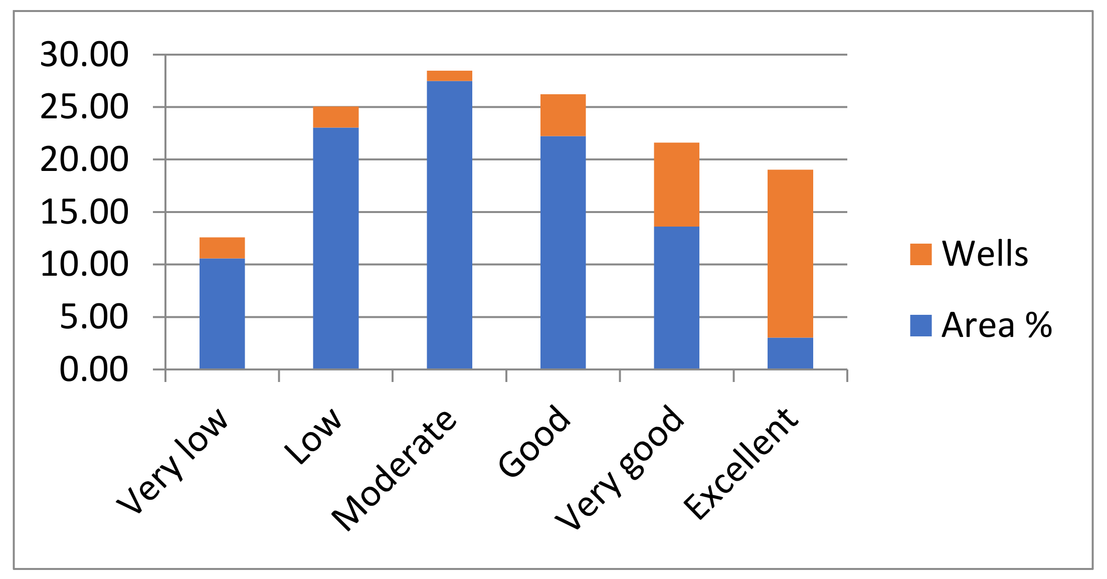
| S.No | Zone | GWPZ % | Wells |
|---|---|---|---|
| 1 | Very low | 10.59 | 2 |
| 2 | Low | 23.06 | 2 |
| 3 | Moderate | 27.47 | 1 |
| 4 | Good | 22.22 | 4 |
| 5 | Very good | 13.62 | 8 |
| 6 | Excellent | 3.03 | 16 |
Publisher’s Note: MDPI stays neutral with regard to jurisdictional claims in published maps and institutional affiliations. |
© 2022 by the authors. Licensee MDPI, Basel, Switzerland. This article is an open access article distributed under the terms and conditions of the Creative Commons Attribution (CC BY) license (https://creativecommons.org/licenses/by/4.0/).
Share and Cite
Sun, T.; Cheng, W.; Abdelkareem, M.; Al-Arifi, N. Mapping Prospective Areas of Water Resources and Monitoring Land Use/Land Cover Changes in an Arid Region Using Remote Sensing and GIS Techniques. Water 2022, 14, 2435. https://doi.org/10.3390/w14152435
Sun T, Cheng W, Abdelkareem M, Al-Arifi N. Mapping Prospective Areas of Water Resources and Monitoring Land Use/Land Cover Changes in an Arid Region Using Remote Sensing and GIS Techniques. Water. 2022; 14(15):2435. https://doi.org/10.3390/w14152435
Chicago/Turabian StyleSun, Tong, Wuqun Cheng, Mohamed Abdelkareem, and Nasir Al-Arifi. 2022. "Mapping Prospective Areas of Water Resources and Monitoring Land Use/Land Cover Changes in an Arid Region Using Remote Sensing and GIS Techniques" Water 14, no. 15: 2435. https://doi.org/10.3390/w14152435