
Flash Flood Susceptibility Mapping in Sinai, Egypt Using Hydromorphic Data, Principal Component Analysis and Logistic Regression


1
Civil Engineering Department, Faculty of Engineering, Minia University, Minia 61111, Egypt
2
Civil Engineering Department, College of Engineering, Shaqra University, Dawadmi 11911, Ar Riyadh, Saudi Arabia
3
Civil Engineering Department, Faculty of Engineering, South Valley University, Qena 83523, Egypt
4
Department of Hydrology and Hydraulic Engineering, Vrije Universiteit Brussel, Pleinlaan 2, 1050 Brussels, Belgium
*
Author to whom correspondence should be addressed.
Water 2022, 14(15), 2434; https://doi.org/10.3390/w14152434
Submission received: 11 June 2022
/
Revised: 24 July 2022
/
Accepted: 1 August 2022
/
Published: 6 August 2022
(This article belongs to the Special Issue Flash Floods: Forecasting, Monitoring and Mitigation Strategies)
Abstract
:Flash floods in the Sinai often cause significant damage to infrastructure and even loss of life. In this study, the susceptibility to flash flooding is determined using hydro-morphometric characteristics of the catchments. Basins and their hydro-morphometric features are derived from a digital elevation model from NASA Earthdata. Principal component analysis is used to identify principal components with a clear physical meaning that explains most of the variation in the data. The probability of flash flooding is estimated by logistic regression using the principal components as predictors and by fitting the model to flash flood observations. The model prediction results are cross validated. The logistic model is used to classify Sinai basins into four classes: low, moderate, high and very high susceptibility to flash flooding. The map indicating the susceptibility to flash flooding in Sinai shows that the large basins in the mountain ranges of the southern Sinai have a very high susceptibility for flash flooding, several basins in the southwest Sinai have a high or moderate susceptibility to flash flooding, some sub-basins of wadi El-Arish in the center have a high susceptibility to flash flooding, while smaller to medium-sized basins in flatter areas in the center and north usually have a moderate or low susceptibility to flash flooding. These results are consistent with observations of flash floods that occurred in different regions of the Sinai and with the findings or predictions of other studies.
1. Introduction
Flash floods are among the deadliest natural disasters in the world, responsible for 85% of inundations and a high death rate of more than 5000 people lost each year [1]. Egypt has experienced many flash floods with loss of life and serious damage to vital infrastructure and buildings, especially in the Sinai, the north coast and the Red Sea coast. Well-known examples are the 1979 flash flood in El-Quseir and Marsa Alam, which killed 19 and destroyed a coastal road along the Red Sea, the flash flood in Marsa Alam in 1991, the flash flood in Alexandria in 1993, which killed 21, and the flash flooding in Assiut in November 1994 resulting in loss of life and infrastructure [2]. Recently, in 26–27 October 2016, heavy rainfall in Ras Gharib on the Red Sea coast resulted in flash flooding that killed dozens and caused damage to infrastructure and property [3]. On 14 November 2019, heavy rains led to flooding in wadi El-Sukkari and further to the Idfu-Marsa Alam Road, fortunately without losses [4].
Sinai in particular is a flood-prone area where flash floods cause significant damage to infrastructure, displacement of populations and sometimes loss of life. An overview of major floods in the Sinai in the past is given by Abdel-Fattah et al. [5] and Omran [6]. Most devastating was the severe flooding in Wadi El-Arish on 17–18 January 2010, which resulted in six deaths and dozens of injuries and vital infrastructure and hundreds of houses destroyed [7]. Cools et al. [8] reported that out of 20 significant rainfall events over a 30-year period (1979–2010) in wadi Watir, located in Southeast Sinai, nine resulted in flash flooding, some of which caused severe damage to the coastal road between Nuweiba and Taba, which was completely washed away in some parts. More recently, a catastrophic flash flood in October 2016 caused many deaths and injuries and damage to roads and buildings in wadi Dahab in South Sinai [9]. El-Fakharany and Mansour [10] discussed dangerous flash flood locations in southern Sinai, including the wadis Werdan, Sedri, El-Aawag and Feiran.
Reliable and accurate data on flash flooding in arid environments are often lacking due to the remoteness and sparse habitation of such areas. Therefore, morphometric analyzes are often used instead to analyze the drainage behavior of such areas. Quantitative measurements of the geometrical features of drainage basins, such as basin size and shape, drainage network and relief form the basis of hydro-morphometric analysis as set forth in the classical works of Horton [11,12], Smith [13], Strahler [14,15] and Schumm [16]. Since the development of remote sensing (RS) and geographic information systems (GIS), hydro-morphological parameters can be easily obtained.
A comprehensive overview of past developments in the analysis of flood risk assessment has been provided by Diaconu et al. [17]. An overview of flash flood risk assessment based on morphometric analyses has been provided by Ali et al. [18], discussing flash flood hazard vulnerability and risk assessment approaches, uncertainties and challenges. Notable recent studies are as follows. Farhan et al. [19] presented a morphometric analysis and flash floods assessment for drainage basins of the Ras En Naqb Area, South Jordan. Mahmood and Rahman [20] studied the flash flood susceptibility modeling using geomorphometric and hydrological approaches in Panjkora Basin, Eastern Hindu Kush, Pakistan. Mahmood and Rahman [21] modeled the flash flood susceptibility using a geomorphometric ranking approach in the Ushairy Basin, in eastern Hindu Kush, Pakistan. Bhat et al. [22] presented a flood hazard assessment of the upper Jhelum basin using morphometric parameters. Obeidat et al. [23] performed a morphometric analysis and prioritized watersheds for flood risk management in the Wadi Easal Basin, Jordan. Pangali Sharma et al. [24] identified potential flash flood areas using a geomorphic approach in the East Rapti River Basin of Nepal.
Hydro-morphometric analyzes have been applied in studies for flood assessment in Egypt. Arnous et al. [25] reported that morphometric analysis strongly supported a high probability of flash flooding in the western part of the Gulf of Suez. Youssef et al. [26] used morphometric parameters to estimate the risk of flash flooding along the St. Katherine Road in southern Sinai. Abdel-Lattif and Sherief [27] used three morphometric parameters (bifurcation ratio, drainage density and stream frequency) to estimate flood hazard in wadi Sudr and wadi Wardan, Gulf of Suez. Elewa et al. [28] presented a hydro-morphometric analysis for the El-Arish Basin in northern and central Sinai to identify suitable sites for collecting runoff. Abdalla et al. [29] presented a geomorphometric classification of wadis along the southeastern Red Sea coast in Egypt, showing that most basins are highly susceptible to flash flooding. Abdel Ghaffar et al. [30] evaluated the flash flood hazard of wadi El-Arish by combining nine morphometric parameters using priority values and classification into high, medium and low hazard. Abuzied et al. [31] used morphometric parameters to evaluate flood sensitive basins and to map the flash flood susceptibility in the Nuweiba area, Sinai. Abdelkareem [32] derived a flash flood hazard map for the wadi Asyuti basin in the eastern desert of Egypt by ranking and combining morphometric parameters that favor higher flood peaks and runoff. Elsadek et al. [33] presented a morphometric analysis to estimate flood hazard in the wadi Qena basin. Abuzied and Mansour [34] combined normalized values of morphometric parameters to obtain hazard indices for sub-basins of wadi Dahab, Sinai. Elsadek et al. [35] investigated flood hazard in wadi Qena based on a combination of morphometric parameter ranking. Kamel and Arfa [4] used a ranking method of 13 morphometric parameters to derive the degree of flash flood hazard of basins between Marsa Alam and Abu Ghuson along the Red Sea coast. Prama et al. [9] derived a flood hazard map for the Dahab region in southern Sinai, by an unweighted combination of normalized morphometric parameters. El-Fakharany and Mansour [10] evaluated morphometric parameters and the occurrence of flash floods in wadi El-Aawag in southwestern Sinai.
The main aim of this research is to quantify the risk of flash flooding in the Sinai Peninsula, Egypt. Various methods are used for this: (1) hydro-morphometric features are derived that are relevant for estimating the sensitivity to flash flooding using satellite images and spatial analysis tools; (2) principal component analysis is applied to reveal relationships between the different catchment properties and to identify the most significant hydro-morphometric parameters; (3) the probability of flash flooding is estimated by logistic regression using observed events of flash floods as dependent variable and the significant principal components of the hydro-morphometric parameters as explanatory variables; (4) prediction results are cross-validated to assess and prove the robustness of the modeling approach; (5) the logistic model is used to generate a map of flash flood probability for the Sinai Peninsula. The novelty of the approach consists primary in generating a flood susceptibility map for the entire Sinai Peninsula, which has not been presented before; previous studies [9,10,26,27,28,30,31,34] only considered only some local sub-basins. A complete flash flood susceptibility map for the Sinai Peninsula can be useful to authorities and decision makers for an overall impact assessment and can contribute to flash flood management and to the planning and implementation of mitigation measures. This study also aims to demonstrate how hydro-morphometric parameters can be used for flood risk assessment in Egypt through a combination of principle component analysis and logistic regression that is robust, reliable and validated. To date, most flood susceptibility studies conducted in Egypt have used a ranking method proposed by Davis [36] to derive flash flood hazard from hydro-morphometric data, by standardizing morphometric parameters, usually in the range of 1 to 5, and then combining and classifying them into groups ranging from lowest to highest risk level [25,26,27,28,29,30,31,32,33,34,35]. However, the number of parameters can vary, all parameters are treated with the same weight as if they have an equal impact on flooding, and the classification into hazard classes is done without rules or standards. In addition, the results are usually not validated.
2. Materials and Methods
2.1. Study Area
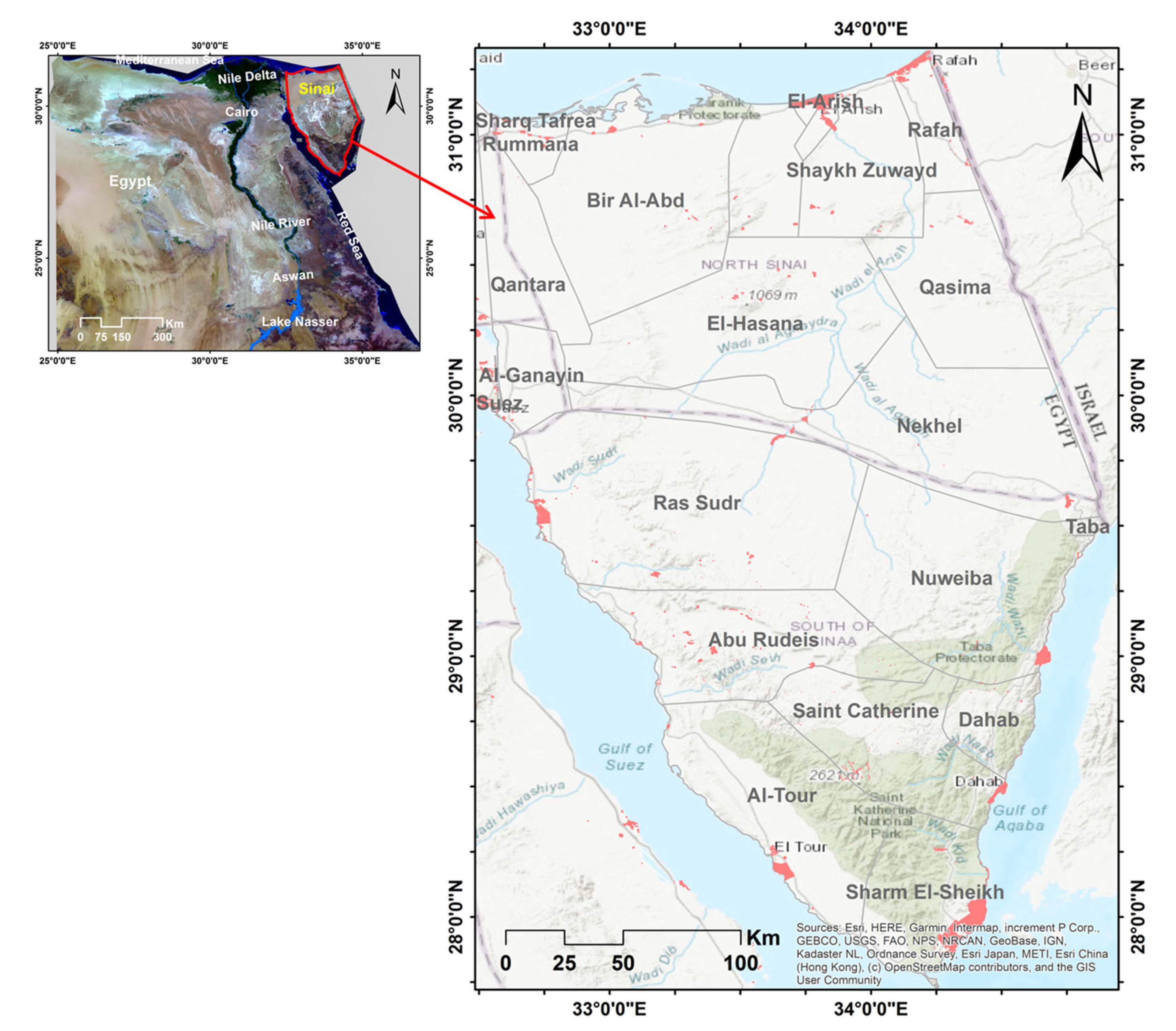
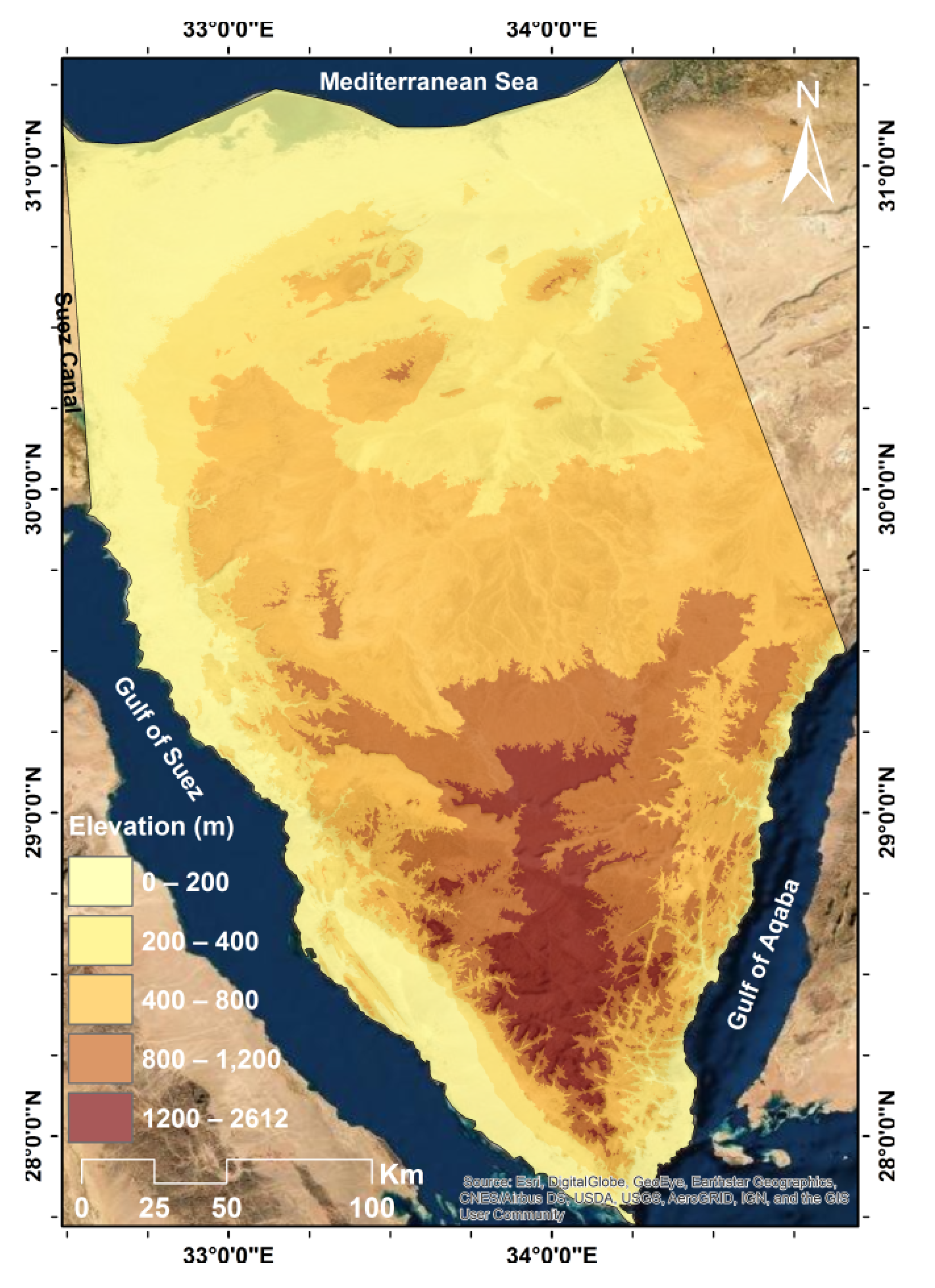
The Sinai Peninsula is located in the northeastern part of Egypt between 32.5–34.8° E and 27.8–31.3° N (Figure 1). It is about 61,000 km2 in size and its largest dimensions are about 385 km from north to south and 210 km from west to east. Geographically, Sinai can be divided into three parts. The northern part consists of broad coastal plains with fossil beaches and extensive sand dunes, some of which are more than 100 m high. The main part is the wadi El-Arish basin which descends from an altitude of more than 900 m to the Mediterranean Sea and forms the largest valley of the Sinai Peninsula. The center is highland mainly composed of two limestone plateaus, El-Tih in the south and El-Egma in the north, where the sources of the wadi Al-Arish arise. The southern part consists of high and rugged mountain ranges of igneous rock, reaching more than 2400 m, with Mount Catherine at 2642 m above sea level being the highest point in Egypt.
Sinai is characterized by a Mediterranean climate in the north and an arid to semi-arid climate in the center and south. In general, summer is very hot and dry, while most rain falls in winter with occasional heavy rainfall combined with thunderstorms. The amount of precipitation decreases from north to south. Most rain falls in a narrow strip along the Mediterranean Sea with values of more than 200 mm/year; further inland the rainfall varies from 100 to 200 mm per year in the north, while in the center and south this usually less than 100 mm per year. Since the potential evaporation demand far exceeds rainfall, there are no real streams or rivers but only ephemeral riverbeds, referred to as wadis, which are generally dry but discharge drainage water after heavy rainfall usually in winter. Wadi El-Arish is the main drainage system to the Mediterranean in the north and center of Sinai. There are several smaller wadis in the south, some of which are known for flash floods, such as Watir, Dahab and Kid in the east which flow into the Gulf of Aqaba and Ras Sudr, Werdan, Feiran, Sedr, Gharandal and Meiar in the west which flow into the Gulf of Suez [6].
2.2. Hydro-Morphometric Parameters
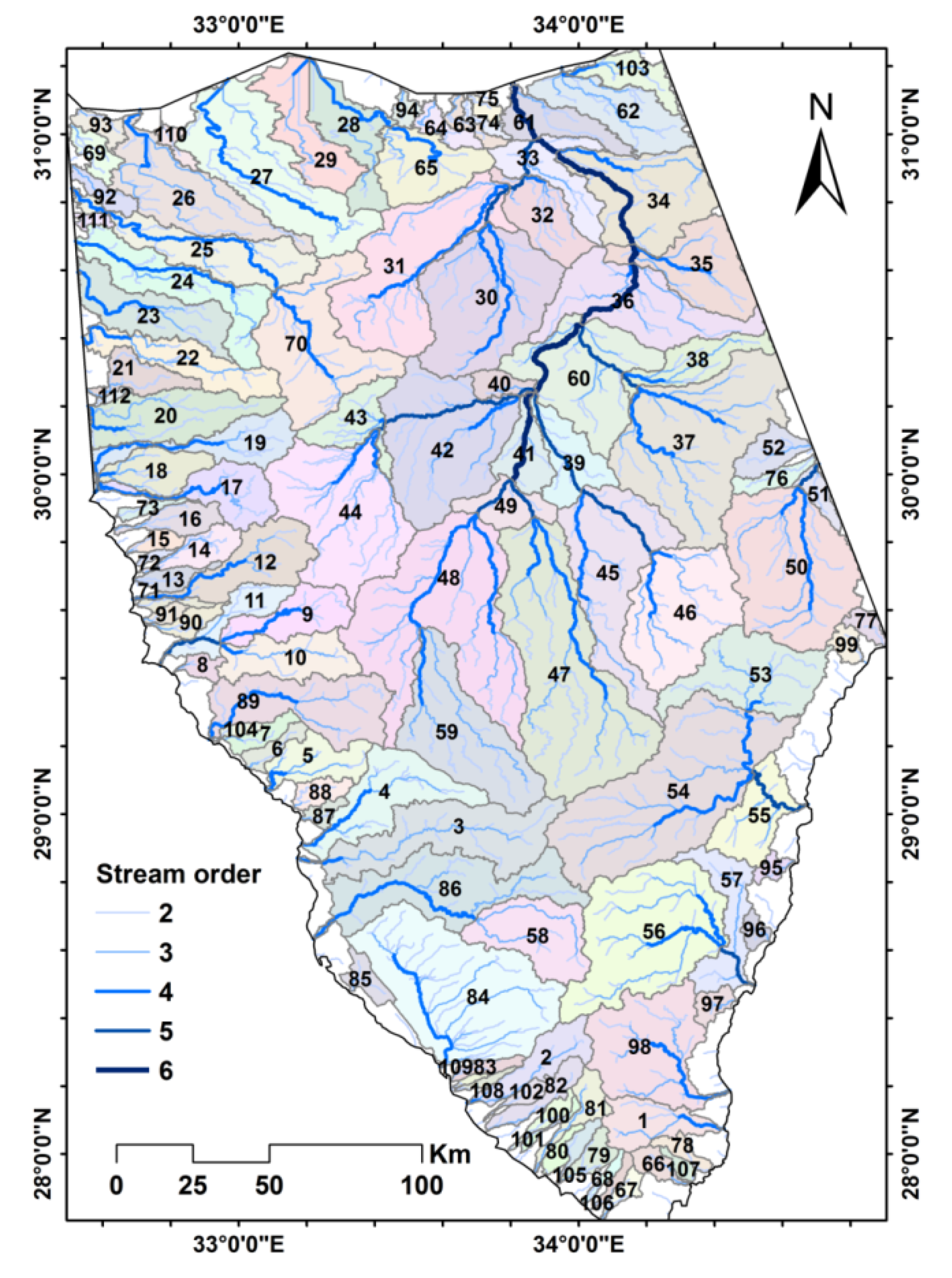
An ASTER Global Digital Elevation Model (DEM) version 3 was downloaded from the NASA Earthdata website (Available online: https://search.earthdata.nasa.gov; accessed on 15 September 2021). The DEM has a latitude and longitude resolution of 1 arc-second (~30 m), and the elevation data have a resolution of 1 m and an accuracy of approximately 10 m [37]. Topographic elevations in the Sinai range from zero to 2612 m above mean sea level as shown in Figure 2. ArcGIS spatial analysis tools are utilized to delineate watersheds and determine their hydro-morphometric parameters. The drainage network is extracted from the DEM using the stream order method of Strahler [31] with a threshold of 4.5 km2 for the upslope drainage area as the starting point of first order streams, which corresponds 5000 grid cells, a standard recommended by ArcGIS spatial analysis tools (Available online: https://pro.arcgis.com; accessed on 22 January 2022). Sub-basins are delineated based on stream orders and hydro-morphometric parameters are derived for each sub-basin using standard spatial analyses methods and equations as listed in Table 1.
Three groups of parameters are considered. The basin geometry group includes six parameters:
- Area (A): surface of a drainage basin, which is a prime determinant of the total discharge [31]; large catchments receive more precipitation and have a higher peak discharge compared to smaller catchments.
- Perimeter (P): circumference of a drainage basin; there are no clear indications of direct significance for the hydrological regime, but it is used in the determination of other parameters.
- Basin length (Lb): maximum distance from the catchment boundary to the outlet; a good indicator of the concentration time of a flood wave [11].
- Form factor (Ff): ratio of the width to the length of a catchment and indicative of the flood regime [11]; large form factors lead to shorter lag times and a higher peak discharge.
- Elongation ratio (Re): ratio of the diameter of a circle with the same area as the catchment area to the maximum catchment length [16]; low values mean less circular shape and longer flood concentration time.
The basin drainage network group includes eight parameters:
- Stream order (Su): highest stream order in a basin according to the method designed by [14]; it is an indicative parameter of the basin dimensions, channel size and stream discharge.
- Stream number (Nu): total number of stream segments of all orders [15]; a high stream number is expected to imply faster peak flow.
- Bifurcation ratio (Rb): average ratio between the number of streams of one order and those of the next higher order [12]; indicative of the complexity of a catchment, but according to [14] less so for the flow regime, although [12] considers flooding more likely in catchments with a higher bifurcation ratio.
- Drainage density (Dd): length of streams per unit area; an indicator of infiltration and permeability of a drainage [11].
- Length of overland flow (Lo): the average length of overland flow is equal to the reciprocal of twice the drainage density [16]; low values indicate shorter flow paths, making the basin more prone to flash flooding.
- Texture ratio (Rt): total number of first order streams per basin circumference; indicates coarse, medium, or fine textured topography [40].
The basin relief group includes four parameters:
- Basin relief (Rf): height difference of the lowest and highest points of a basin and an essential indicator of surface runoff [16].
- Relief ratio (Rr): ratio of the basin relief to the basin length and a key element for understanding erosion and drainage [16].
- Ruggedness number (Rn): product of drainage density and basin relief; regions prone to flash flooding have higher ruggedness numbers, indicating high drainage density combined with steep slopes [38].
- Mean basin slope (S): major factor controlling infiltration and surface runoff and the resulting runoff rate and concentration time.
2.3. Principal Component Analysis
Before creating a predictive model, principal component analysis (PCA) [41] is used as an exploratory data analysis to identify the relevant information in the hydro-morphometric data set. PCA linearly transforms the data into orthogonal uncorrelated variables known as principal components (PCs), which preserve the total variance in the original data
where are the principal components, are the scores of the linear transformation, are the standardized hydro-morphometric parameters, and is the number of parameters. Note that the hydro-morphometric parameters are standardized to remove any effect of scale and units of the observations by subtracting the sample mean and dividing by the sample standard deviation. It can be shown that the principal components are the eigenvectors of the correlation matrix of the data and that the associated eigenvalues give the variance explained by each eigenvector [41]. The eigenvectors are ordered in descending order of the eigenvalues and PCs with eigenvalues smaller than one are ignored because they contain less information than the original variables, which reduces the dimensionality of the data. The scores that relate the remaining PCs to the original parameters provide information about the impact and relevance of the original parameters on the overall information in the data set. In practice, correlation coefficients between the PCs and the original parameters are used to explain and interpret the strength of the relationships. Large (either positive or negative) correlation coefficients indicate that a parameter has a strong effect on that principal component. The interpretation is enhanced by Varimax rotation, which aligns the PCs in directions highlighting the relationships between the PCs and the observed data [41].
2.4. Logistic Regression
A logistic model is used to predict the probability of a flash flood
where logit is the logistic function (natural logarithm of the odds), is the probability, is the model intercept, are the model coefficients, are the predictors (explanatory parameters), and is the number of predictors. The logistic model is used to predict the occurrence of a flash flood in a basin using observed characteristics of the basin as predictors. Since there are too many hydro-morphometric parameters to use as predictors, we will instead consider the significant PCs of the basin hydro-morphometric data as predictors. The logistic model predicts the flood probability which can be used to assess the susceptibility of a basin to flash flooding.
The model coefficients are estimated by logistic regression. For this, we use observations of flash floods reported in the literature [5,6,8,9,10]; basins where flooding has been observed are shown in Table 2. The observed probability of flooding is set to one for these basins, while for the other basins the probability is zero. Flash floods in Wadi El-Arish were excluded in the analysis because Wadi El-Arish consists of many sub-basins, while the exact location of the floods was usually not clearly observed or reported because Wadi El-Arish is so vast and sparsely populated.
The model coefficients are estimated by fitting the model to these observations using maximum likelihood, for which we use the glm generalized maximum likelihood fitting procedure of the R Stats package for statistical computing [42]. The goodness of fit is assessed by the deviance, a measure of the likelihood, and the quality of the model by the Akaike information criterion (AIC) [43], a trade-off between the goodness of fit and the complexity of the model. The significance of each predictor is verified by removing each predictor one at the time, re-estimating the model coefficients with the remaining predictors and comparing the resulting deviance and AIC with the original model. The reliability of the model is also verified by cross-validation where observed flood events are removed one by one, model coefficients are re-estimated by logistic regression with the remaining data and the flood probability is predicted for the removed event and compared to what was obtained with the original model.
3. Results
3.1. Drainage Catchments and Hydro-Morphometric Data
The drainage network obtained from the DEM is shown in Figure 2 and consists of 112 sub-basins of different sizes and shapes, as shown in Figure 3. Large basins such as wadis El-Arish, Feiran, Dahab and Watir are subdivided to obtain a more or less uniform spatial distribution of the sub-basins over the area. Values of the hydro-morphometric parameters for each basin are given in Table S1 in the Supplementary Materials. An overview of the range of the hydro-morphometric parameters is given in Table 3, with minimum and maximum values and the mean and standard deviation necessary for standardization of the parameters in the PCA.
3.2. Principal Component Analysis
The results of the PCA are presented in Table 4 and Table 5. Table 4 lists the first eight eigenvalues, and the variance explained by each component, and cumulative variance, both expressed as a percentage of the total variance contained in the data. Significant values are indicated in bold. Only the first four PCs have eigenvalues greater than one, while the fifth eigenvalue is lower but very close to one, and together these account for 90% of the variation in the data. Therefore, the other PCs can be ignored. Table 5 lists the correlation coefficients between the first five PCs and the hydro-morphometric parameters after Varimax rotation; the corresponding scores are given in Table S2 in the Supplementary Materials. Significant values in Table 5 are shown in bold. The first component is highly correlated with several hydro-morphometric parameters: area (A), perimeter (P) and basin length (Lb) which are directly related to the size of a watershed, and with stream order (Su), stream number (Nu), stream length (Lu) and texture ratio (Rt) which are also indirectly related to size. Thus, the first and most important principal component represents the effect of basin size and accounts for 37% of the variation in the data. The second component is strongly correlated with all relief parameters: basin relief (Rf), relief ratio (Rr), ruggedness number (Rn) and mean basin slope (S); this component accounts for 19% of the variation in the data. The third component, which accounts for 15% of the total variance, is strongly correlated with drainage density (Dd) and length of overland flow (Lo). This component thus represents the drainage capacity of a river basin. The fourth component accounts for 14% of the total variance and is strongly correlated with the form factor (Ff), compactness coefficient (Cc) and elongation ratio (Re), so this component expresses the influence of the basin shape. The fifth component accounts for only 5% of the variance but is rather special in that it is only significantly correlated with the bifurcation ratio (Rb). Thus, this component represents the effect of stream bifurcation, which is apparently a unique basin property unrelated to any other hydro-morphometric parameter. Note that the stream frequency (Fs) is not significantly correlated with any of the PCs and thus contributes little to the information contained in the data. Principal component values for all basins are given Table S3 in the Supplementary Materials.
3.3. Logistic Regression
Results of the logistic regression with the PCs as predictors are given in Table 6. The table shows the estimated model coefficients, the standard error, z-value (coefficient divided by standard error) and the probability that the predictor is statistically significant, for which it is common practice to prescribe a value less than 0.05 for a normal distribution. Note that this is only the case for PC1 and PC4 and not for PC3 and PC5, while PC2 is very close to the threshold. However, the assumption of a normal distribution is not reliable if the sample size is small, as in this case. The next two columns in the table provide the deviation and AIC values, which indicate how well the model with the selected predictors fits the observations. The values corresponding to the intercept are for the null model, which is a logistic model with only an intercept and no predictors that is used as a reference to compare with other models. The values corresponding to the predictors are for excluding that predictor from the full model and the values on the last line are for the total full model. Both the deviance and AIC should be as small as possible. Comparison of the deviance and AIC obtained for the total model and for the null model shows a large difference, indicating that the predictors allow significant improvement in goodness of fit. Comparison of the deviance and AIC when one of the predictors is removed from the full model shows that all predictors are relevant and should not be removed from the model. The increase in deviance when one of the predictors is removed compared to the full model also indicates the importance of that predictor in the model. It follows that the order of importance of the predictors is: PC1, PC4, PC2, PC5 and PC3, as given in the last column of Table 6.
Results of the cross-validation where observed flood events are removed one by one, and the recalibrated model is used to predict the flood probability for the removed event are given in Table 7. This shows that after removing one of the observed flood basins, the model proves to be robust because the estimates of flood probability remain in the same range as predicted with the original model.
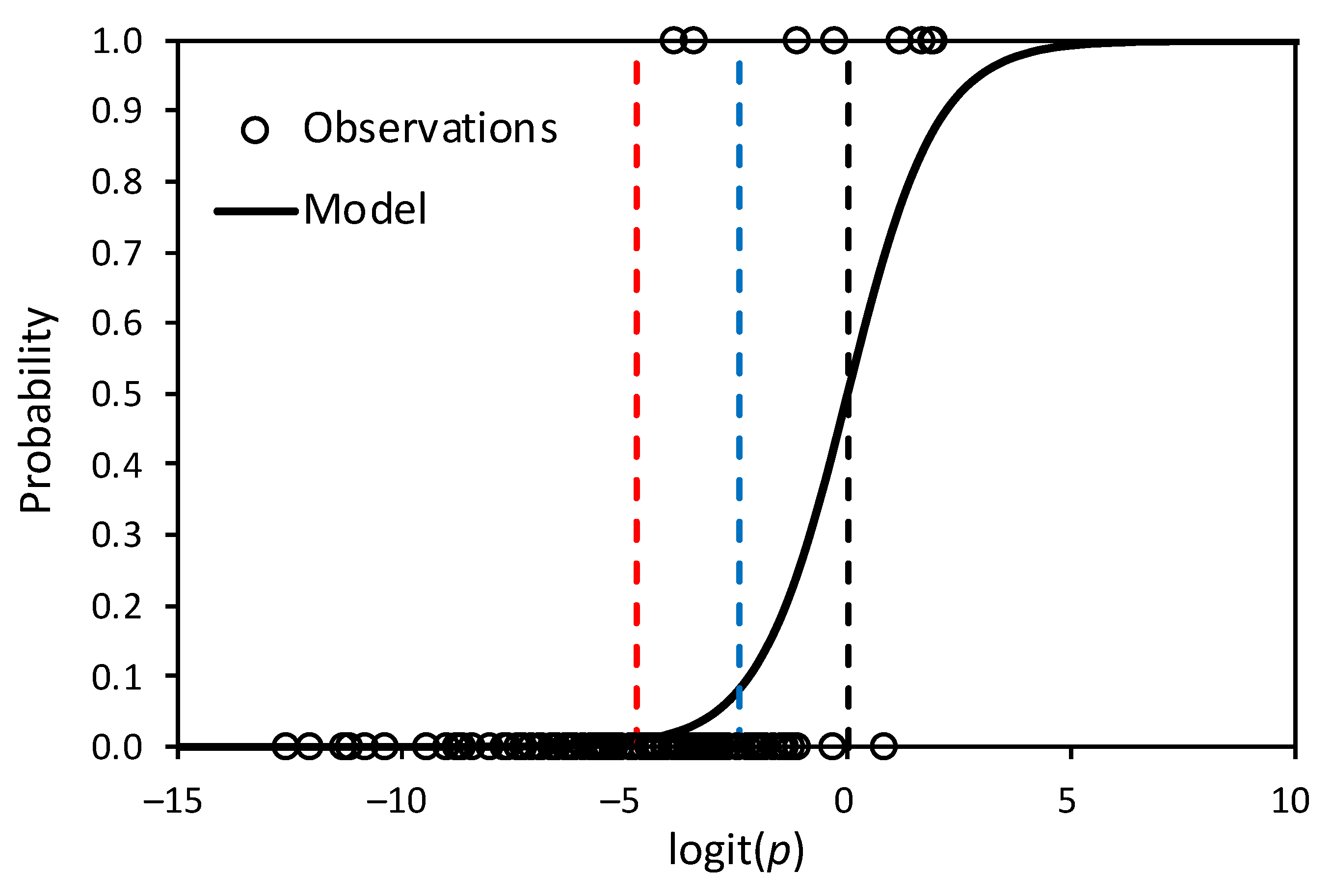
The flood probability predicted by the logistic model for all basins is shown in Table S4 in the Supplementary Materials. A comparison between the flood probability predicted by the logistic model and the observations is shown in Figure 4.
The nine basins where flash floods were observed are shown in the upper part of the graph (p = 1) and the 103 basins where no floods were observed in the lower part (p = 0). The solid line represents the logistic model that fits the observations as closely as possible but has to compromise in the middle part of the graph where basins with observed flooding overlap with basins where no flooding has been observed. Since there are many more basins where no flooding has been observed, the logistic model is strongly conditioned by the non-flooding events, as can be clearly seen in the graph. This should be taken into account when evaluating the model results and selecting threshold values to identify the flood prone basins. The red dotted line in the graph represents the mean outcome predicted by the model given by the intercept, logit(p) = c0 = −4.74 (Table 6). Note that all basin where floods have been observed are on the right side of this line, while all basins predicted by the model on the left of this line have a near zero predicted flooding probability. Basins predicted to the right of the red line are thus prone to flooding with a probability that increases the further they are from this line. The blue dotted line in the graph shows the average outcome of the observations, logit(p) = ln(9/103) = −2.44. All basins plotted to the right of this line have a higher probability of flooding than is observed on average, and vice versa. Seven of the basins where flash floods have been observed are to the right of this line. Additionally, to the right of this line are 15 basins where no flooding has been observed, so these basins have features that indicate a higher probability of flash flooding than observed. The black dotted line represents logit(p) equal to zero (p = 0.5). There are only six basins with a predicted logit(p) greater than zero (p > 0.5) and thus very sensitive to flash flooding; five of these, wadis Kid, El-Aawag, Feiran upstream, Dahab and Watir, are basins where flooding has been observed and one, wadi Feiran downstream, where no flooding has been assumed but has similar characteristics to the other five.
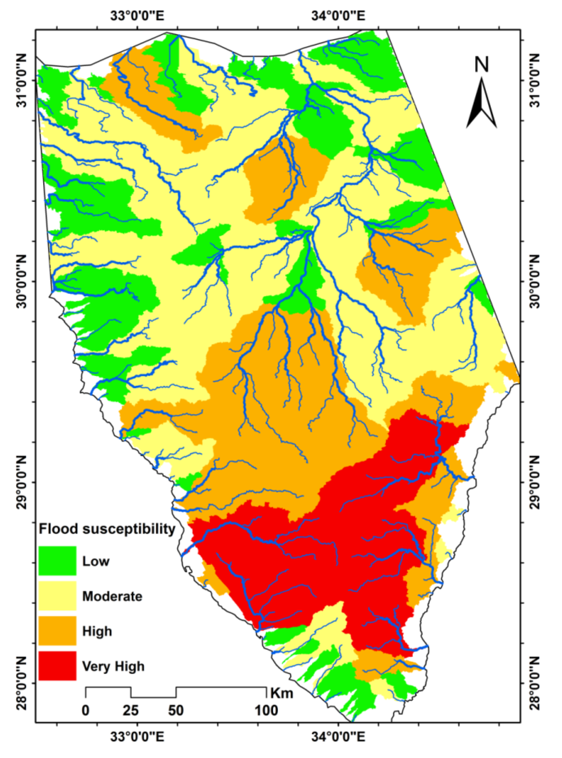
The above considerations are used to classify the flash flood susceptibility of all basins. Flood sensitivity classes are defined as follows: logit(p) < −4.74 is low sensitivity to flooding, −4.74 < logit(p) < −2.44 is moderate sensitivity, −2.44 < logit(p) < 0 is high sensitivity and logit(p) > 0 is very high sensitivity. The resulting map with the sensitivity of all basins is shown in Figure 5.
4. Discussion
Results of the PCA (Table 5) indicate that the hydro-morphometric characteristics of the Sinai drainage basins can be combined into five groups that account for 90% of the variation of the data and have clear physical meaning. Ordered in decreasing importance in explaining the total variance, the first group includes all hydro-morphometric parameters related to size, the second group consists of parameters related to relief, the third group of parameters relates to basin shape, the fourth group of parameters relates to drainage capacity and the fifth group consists only of the bifurcation ratio. However, the importance of the basin characteristics on flash flood occurrence is not in order of explained variance in the data, but in a different order based on flash flood prediction, as shown by the logistic regression (Table 6). Most important in predicting flash flooding is the basin size, followed by drainage density, relief, bifurcation ratio and basin shape. The latter two are not statistically significant in the model regression, but nevertheless appear to be relevant in terms of likelihood combined with model complexity (AIC, Table 5), and therefore should not be removed from the model. The importance of a predictor is given by the regression coefficients (Table 5). It follows that basin size and drainage density are about two times more important than relief, stream bifurcation or basin shape.
Not surprisingly, the size of a basin is the most important factor in predicting flash flooding. In the case where local thunderstorms are more or less spatially random, the probability of an extreme thunderstorm in a large basin will be greater than in a small basin, increasing the risk of flash flooding in large basins. Equally important is the converse that less or no flash flooding is observed in small basins. The PC representing the drainage density is the second most important predictor of flash flooding, but surprisingly the regression coefficient is negative, so that the flood probability decreases with increasing drainage density, which is contradictory to what is commonly believed. The reason is that flash flooding and drainage density are examined here on a regional scale. Locally, higher drainage density may result in faster drainage, but this is not necessarily the case when comparing drainage densities of basins of different sizes and characteristics. The drainage density of basins expresses how channels and surrounding floodplains are spatially arranged, which is strongly determined by the shape, size and relief of the basin. A low drainage density can indicate large, compact basins with a strong relief, and on the other hand, a high drainage density can indicate small basins with flat elongated or dispersed floodplains. In the present case, the values of the drainage densities for all basins where flash flooding have been observed vary between 0.38 and 0.47, which is below average (Table 3); these basins are also large with a strong relief and compact shapes.
Relief is only the third most important factor after basin shape and drainage density, which is somewhat unexpected, as relief is usually considered one of the most important factors for flooding [18]. The fourth predictor relates to the bifurcation ratio, which appears to be a unique but minor factor in flash flood prediction that, however, is often ignored in other studies presented in the literature. The last and least important predictor relates to the shape of basins, where, as expected, compact basins are more prone to flooding than elongated bases.
Comparison of these results with results of similar studies in other countries or in Egypt [19,20,21,22,23,24,25,26,27,28,29,30,31,32,33] is fruitless, as all these studies were performed on a much smaller scale than the current study, usually only one basin, and no analysis of variance such as principal components was applied to establish relationships between hydro-morphometric parameters and to identify key parameters related to the total variance, and importantly, no observations of occurring flash floods were used to reveal the predictive power of the parameters to flooding. Therefore, this study shows that a large set of hydro-morphometric parameters can be reduced to a much smaller set without loss of information, indicating redundancy in the data. So, hydro-morphometric parameters are not independent and do not add more information by their number. Therefore, in flood sensitivity analyses, it makes no sense to combine correlated factors that express similar characteristics, as is done in traditional ranking methods where all parameters are combined with the same weight.
The flash flood susceptibility map (Figure 5) shows the spatial distribution into four categories: very high, high, moderate and low susceptibility. The very high sensitivity zone is located in the mountain ranges of the southern Sinai and consists of six major basins known for their flash flooding, such as wadis El-Aawag, Feiran and Kid and the upstream sub-basins of wadis Dahab and Watir, which in total represent an area of approximately 8000 km2, or 15% of the total area of Sinai. The high sensitivity zone is mainly in the center of the Sinai Peninsula and some scattered areas further north. It encompasses 16 river basins, covering a total area of approximately 15,000 km2 or 28% of the Sinai area, including some upstream sub-basins of wadi El-Arish, sub-basins of wadi Dahab and Watir, and the basins of wadis Sedri, Garf and Werdan which drain into the Gulf of Suez. The basins in the north are wadi El-Beada in Bir Al-Abd, which drains to the Mediterranean, and two sub-basins of wadi El-Harish in El-Hasana and Quasisma, respectively, which may be the source of the flash floods that have been observed in this wadi. The moderate sensitivity zone is mainly located in the north of the Sinai Peninsula and includes 36 watersheds with a total area of about 21,000 km2 or 39% of the Sinai area. These are usually smaller to medium sized basins located in flatter areas. The low-sensitive zone comprises 45 catchments with a total area of approximately 10,000 km2, or 18% of the Sinai area. These are usually very small basins on flat terrains with short drainage paths and few branches. Most are located in the north and center along the periphery of the Sinai Peninsula; some are also found in the southern part of Sinai. The resulting flash flood sensitivity map is largely consistent with flash flood observations that occurred in different regions of the Sinai and with the findings or predictions of other studies [6,9,10,31,34].
In particular, the map indicates the high probability of flash flooding in the mountainous basins of southern Sinai, as observed and reported in several publications, such as wadi Feiran [26], wadi Watir [8,31], wadi Dahab [9] and wadi El-Aawag [10]. The map also indicates the high or moderate sensitivity of some basins in southwestern Sinai draining to the Gulf of Suez as described in the literature, such as wadi Sedri [10], wadi Sudr and wadi Wardan [27]. By indicating the high sensitivity to flooding of some sub-basins in El-Hasana and Quasisma of wadi El-Arish, the map also sheds light on the possible origin of flash floods observed in El-Aris, as discussed by Moawad [7], Elewa et al. [28] and Abdel Ghaffar et al. [30]. Nevertheless, it is clear that these results can be improved as more accurate and detailed information on the characteristics of river basins and the occurrence of flash floods in the Sinai becomes available.
Flood susceptibility mapping presented by other studies conducted in Egypt or other countries [19,20,21,22,23,24,25,26,27,28,29,30,31,32,33] mainly used a classification method consisting of standardization of the morphometric parameters, usually in the range of 1 to 5, and combining the resulting scores without any ranking or weighting as if all parameters have an equal effect on flooding. In addition, there is no validation of the results with field data regarding the occurrence of flash floods, which makes it impossible to verify such simplifying assumptions and approach. In contrast, the method presented in the present study, combining principal component analysis and logistic regression, proves to be robust, reliable and validated and therefore superior to what has been presented before.
The drainage network extracted from satellite data and the sub-division of large basins introduces some bias regarding the range and magnitude of the derived hydro-morphometric parameters. Subdivision is, of course, necessary to get a map of the spatial distribution of flash flood susceptibility in the Sinai. A more detailed subdivision could improve the resolution and accuracy of such a map, but the uncertainty about the exact location of flash flood observations needed to optimize the logistic regression model could potentially cause more bias and uncertainty. In this regard, the current study is only a first attempt, and more research is needed to assess accuracy and improve results.
5. Conclusions
Thunderstorms in the Sinai Peninsula often lead to flash floods that can cause significant damage to infrastructure and sometimes even loss of life. Therefore, this study shows how to derive the susceptibility to flash flooding using hydro-morphometric characteristics of the watersheds. Subbasins of various sizes and shapes and their hydro-morphometric features are derived from a digital elevation model from NASA Earthdata. Principal component analysis reveals the relationships between the most important hydro-morphometric parameters and allows us to derive five significant principal components that explain 90% of the variation in the data and have clear physical significance: basin size, drainage density, relief, stream bifurcation and basin shape. This shows that hydro-morphometric parameters are not independent which makes traditional ranking methods to estimate flood sensitivity questionable.
The flash flood probability can be estimated by logistic regression using the significant principal components as predictors and the model coefficients estimated by fitting the model to flash flood observations using maximum likelihood. Cross-validation proves that the model is robust because the estimates of flood probability remain similar to those predicted with the original model. The model shows that the size of a basin is the most important factor in predicting flash flooding, followed by drainage density, relief, bifurcation ratio and basin shape. The logistic model can be used to classify all basins in Sinai into four classes: low, moderate, high and very high susceptibility to flash flooding. The resulting map indicates that the large basins in the mountain ranges of the southern Sinai have a very high susceptibility to flash flooding, several basins in the southwestern Sinai have a high or moderate susceptibility to flash flooding, some sub-basins of wadi El-Arish in the center have a high susceptibility to flash flooding, while smaller to medium-sized basins in flatter areas in the center and north usually have a moderate or low susceptibility to flash flooding. These results are consistent with observations of flash floods that occurred in different regions of the Sinai and with the findings or predictions of other studies.
Supplementary Materials
The following supporting information can be downloaded at: https://www.mdpi.com/article/10.3390/w14152434/s1, Table S1: Values of the hydro-morphometric parameters for each basin; Table S2: PCA scores after Varimax rotation; Table S3: Values of the principal components; Table S4: Predicted probability for flash flooding.
Author Contributions
Conceptualization, M.E.-R. and W.M.E.; methodology, M.E.-R. and F.D.S.; validation, M.E.-R. and F.D.S.; data curation, M.E.-R. and W.M.E.; writing—review and editing, M.E.-R. and F.D.S.; visualization, M.E.-R.; supervision, M.E.-R. All authors have read and agreed to the published version of the manuscript.
Funding
This research received no external funding.
Institutional Review Board Statement
Not applicable.
Informed Consent Statement
Not applicable.
Data Availability Statement
Not applicable.
Conflicts of Interest
The authors declare no conflict of interest.
References
- WMO. World Meteorological Organization: Flash Flood Guidance System (FFGS) with Global Coverage. 2016. Available online: https://community.wmo.int/hydrology-and-water-resources/flash-flood-guidance-system-ffgs-global-coverage (accessed on 1 May 2022).
- El Gohary, R. Environmental Flash Flood Management in Egypt. In Flash Floods in Egypt; Negm, E.E., Ed.; Advances in Science, Technology & Innovation; Springer: New York, NY, USA, 2020; pp. 85–105. [Google Scholar]
- Elnazer, A.A.; Salman, S.A.; Asmoay, A.S. Flash flood hazard affected Ras Gharib city, Red Sea, Egypt: A proposed flash flood channel. Nat. Haz. 2017, 89, 1389–1400. [Google Scholar] [CrossRef]
- Kamel, M.; Arfa, M. Integration of remotely sensed and seismicity data for geo-natural hazard assessment along the Red Sea Coast, Egypt. Arab. J. Geosci. 2020, 13, 1195. [Google Scholar] [CrossRef]
- Abdel-Fattah, M.; Kantoush, S.; Sumi, T. Integrated Management of Flash Flood in Wadi System of Egypt: Disaster Preventing and Water Harvesting. Annu. Disas. Prev. Res. Inst. Kyoto Univ. 2015, 58, 485–496. [Google Scholar]
- Omran, E.-S.E. Egypt’s Sinai Desert Cries: Flash Flood Hazard, Vulnerability, and Mitigation. In Flash Floods in Egypt; Negm, E.E., Ed.; Advances in Science, Technology & Innovation; Springer: New York, NY, USA, 2020; pp. 215–236. [Google Scholar]
- Moawad, M.B. Analysis of the flash flood occurred on 18 January 2010 in wadi El Arish, Egypt (a case study). Geomat. Nat. Haz. Risk. 2013, 4, 254–274. [Google Scholar] [CrossRef] [Green Version]
- Cools, J.; Vanderkimpen, P.; El-Afandi, G.; Abdelkhalek, A.; Fockedey, S.; El-Sammany, M.; Abdallah, G.; El-Bihery, M.; Bauwens, W.; Huygens, M. An early warning system for flash floods in hyper-arid Egypt. Nat. Haz. Earth Syst. Sci. 2012, 12, 443–457. [Google Scholar] [CrossRef]
- Prama, M.; Omran, A.; Schröder, D.; Abouelmagd, A. Vulnerability assessment of flash floods in Wadi Dahab Basin, Egypt. Environ. Earth Sci. 2020, 79, 114. [Google Scholar] [CrossRef] [Green Version]
- El-Fakharany, M.A.; Mansour, N.M. Morphometric analysis and flash floods hazards assessment for Wadi Al Aawag drainage Basins, southwest Sinai, Egypt. Environ. Earth Sci. 2021, 80, 168. [Google Scholar] [CrossRef]
- Horton, R.E. Drainage-basin characteristics. Eos Trans. Am. Geophys. Union 1932, 13, 350–361. [Google Scholar] [CrossRef]
- Horton, R.E. Erosional development of streams and their drainage basins; hydrophysical approach to quantitative morphology. Geol. Soc. Am. Bull. 1945, 56, 275–370. [Google Scholar] [CrossRef] [Green Version]
- Smith, K.G. Standards for grading texture of erosional topography. Am. J. Sci. 1950, 248, 655–668. [Google Scholar] [CrossRef]
- Strahler, A.N. Quantitative analysis of watershed geomorphology. Trans. Am. Geoph. Union 1957, 38, 913–920. [Google Scholar] [CrossRef] [Green Version]
- Strahler, A.N. Quantitative Geomorphology of Drainage Basins and Channel Networks. In Handbook of Applied Hydrology; McGraw Hill Book Company: New York, NY, USA, 1964; p. 411. [Google Scholar]
- Schumm, S.A. Evolution of drainage systems and slopes in badlands at Perth Amboy, New Jersey. Bull. Geol. Soc. Am. 1956, 67, 597–646. [Google Scholar] [CrossRef]
- Diaconu, D.C.; Costache, R.; Popa, M.C. An overview of flood risk analysis methods. Water 2021, 13, 474. [Google Scholar] [CrossRef]
- Ali, K.; Bajracharyar, R.M.; Raut, N. Advances and challenges in flash flood risk assessment: A review. J. Geogr. Nat. Disast. 2017, 7, 195. [Google Scholar] [CrossRef] [Green Version]
- Farhan, Y.; Anaba, O.; Salim, A. Morphometric analysis and flash floods assessment for drainage basins of the Ras En Naqb area, south Jordan using GIS. J. Geosci. Environ. Protect. 2016, 4, 9–33. [Google Scholar] [CrossRef] [Green Version]
- Mahmood, S.; Rahman, A. Flash flood susceptibility modeling using geo-morphometric and hydrological approaches in Panjkora Basin, Eastern Hindu Kush, Pakistan. Environ. Earth Sci. 2019, 78, 43. [Google Scholar] [CrossRef]
- Mahmood, S.; Rahman, A. Flash flood susceptibility modelling using geomorphometric approach in the Ushairy Basin, eastern Hindu Kush. J. Earth Syst. Sci. 2019, 128, 97. [Google Scholar] [CrossRef] [Green Version]
- Bhat, M.S.; Alam, A.; Ahmad, S.; Farooq, H.; Ahmad, B. Flood hazard assessment of upper Jhelum basin using morphometric parameters. Environ. Earth Sci. 2019, 78, 54. [Google Scholar] [CrossRef]
- Obeidat, M.; Awawdeh, M.; Al-Hatouli, F. Morphometric analysis and prioritisation of watersheds for flood risk management in Wadi Easal Basin (WEB), Jordan, using geospatial technologies. Flood Risk Manag. 2021, 14, e12711. [Google Scholar] [CrossRef]
- Pangali Sharma, T.P.; Zhang, J.; Khanal, N.R.; Prodhan, F.A.; Nanzad, L.; Zhang, D.; Nepal, P. A geomorphic approach for identifying flash flood potential areas in the East Rapti River Basin of Nepal. ISPRS Int. J. Geo-Inf. 2021, 10, 247. [Google Scholar] [CrossRef]
- Arnous, M.O.; Aboulela, H.; Green, D. Geo-environmental hazards assessment of the north western Gulf of Suez, Egypt. J. Coast. Conserv. 2011, 15, 37–50. [Google Scholar] [CrossRef]
- Youssef, A.M.; Pradhan, B.; Hassan, A.M. Flash flood risk estimation along the St. Katherine road, southern Sinai, Egypt using GIS based morphometry and satellite imagery. Environ. Earth Sci. 2011, 62, 611–623. [Google Scholar] [CrossRef]
- Abdel-Lattif, A.; Sherief, Y. Morphometric analysis and flash floods of Wadi Sudr and Wadi Wardan, Gulf of Suez, Egypt: Using digital elevation model. Arab. J. Geosci. 2012, 5, 181–195. [Google Scholar] [CrossRef]
- Elewa, H.H.; Ramadan, E.M.; El-Feel, A.A.; Abu El-Ella, E.A.; Nosair, A.M. Runoff water harvesting optimization by using RS, GIS and watershed modelling in Wadi El-Arish, Sinai. Int. J. Eng. Res. Technol. 2013, 2, 1635–1648. [Google Scholar]
- Abdalla, F.; El-Shamy, I.; Bamousa, A.; Mansour, A.; Mohamed, A.; Tahoon, M. Flash floods and groundwater recharge potentials in arid land alluvial basins, southern Red Sea coast, Egypt. Inter. J. Geosci. 2014, 5, 971–982. [Google Scholar] [CrossRef] [Green Version]
- Abdel Ghaffar, M.K.; Abdellatif, A.D.; Azzam, M.A.; Riad, M.H. Watershed characteristic and potentiality of wadi El-Arish, Sinai, Egypt. Int. J. Adv. Remote Sens. GIS 2015, 4, 1070–1091. [Google Scholar]
- Abuzied, S.; Yuan, M.; Ibrahim, S.; Kaiser, M.; Saleem, T. Geospatial risk assessment of flash floods in Nuweiba area, Egypt. J. Arid Environ. 2016, 133, 54–72. [Google Scholar] [CrossRef]
- Abdelkareem, M. Targeting flash flood potential areas using remotely sensed data and GIS techniques. Nat. Haz. 2017, 85, 19–37. [Google Scholar] [CrossRef]
- Elsadek, W.M.; Ibrahim, M.G.; Mahmod, W.E. Flash flood risk estimation of Wadi Qena Watershed, Egypt using GIS based morphometric analysis. Appl. Environ. Res. 2018, 40, 36–45. [Google Scholar] [CrossRef] [Green Version]
- Abuzied, S.M.; Mansour, B.M.H. Geospatial hazard modeling for the delineation of flash flood-prone zones in Wadi Dahab basin, Egypt. J. Hydroinform. 2019, 21, 180–206. [Google Scholar] [CrossRef] [Green Version]
- Elsadek, W.M.; Ibrahim, M.G.; Mahmod, W.E.; Kanae, S. Developing an overall assessment map for flood hazard on large area watershed using multi-method approach: Case study of Wadi Qena watershed, Egypt. Nat. Haz. 2019, 95, 739–767. [Google Scholar] [CrossRef]
- Davis, J. Statics and Data Analysis in Geology; Wiley: New York. NY, USA, 1975. [Google Scholar]
- Abrams, M.; Crippen, R.; Fujisada, H. ASTER Global Digital Elevation Model (GDEM) and ASTER Global Water Body Dataset (ASTWBD). Remote Sens. 2020, 12, 1156. [Google Scholar] [CrossRef] [Green Version]
- Melton, M. An Analysis of the Relations among Elements of Climate, Surface Properties and Geomorphology; Department of Geology, Columbia University, Technical Report, 11, Project NR 389-042; Office of Navy Research: New York, NY, USA, 1957. [Google Scholar] [CrossRef]
- Strahler, A.N. Hypsometric (area-altitude) analysis of erosional topography. Geol. Soc. Am. Bull. 1952, 63, 1117–1142. [Google Scholar] [CrossRef]
- Smith, K.G. Erosional processes and landforms in badlands national monument, South Dakota. Bull. Geol. Soc. Am. 1958, 69, 975–1008. [Google Scholar] [CrossRef]
- Jolliffe, I.T. Principal Component Analysis, 2nd ed.; Springer: New York, NY, USA, 2002. [Google Scholar]
- R Core Team. R: A Language and Environment for Statistical Computing; R Foundation for Statistical Computing: Vienna, Austria, 2017; Available online: http://www.R-project.org/ (accessed on 15 November 2021).
- Akaike, H. A new look at the statistical model identification. IEEE Trans. Autom. Control. 1974, 19, 716–723. [Google Scholar] [CrossRef]
Figure 1.
Location of the study area.

Figure 2.
Topography of the Sinai derived from a digital elevation model from NASA Earthdata.

Figure 3.
Sub-basins with ID number and drainage channels with stream order, excluding first order, derived from the digital elevation model.
Figure 3.
Sub-basins with ID number and drainage channels with stream order, excluding first order, derived from the digital elevation model.

Figure 4.
Predicted and observed flash flood probability against logit(p): dots are observed flash flood probabilities, the solid black line represents the probability predicted by the logistic model, the red dotted line corresponds to the mean of the model predictions, logit(p) = −4.74, the blue dotted line to the mean of the observations, logit(p) = −2.44, and the black dotted line with logit (p = 0.5) = 0.

Figure 5.
Susceptibility to flash flooding in the Sinai predicted with the probabilistic model (Equation (2)) using the principal components of the hydro-morphometric parameters as predictors.
Figure 5.
Susceptibility to flash flooding in the Sinai predicted with the probabilistic model (Equation (2)) using the principal components of the hydro-morphometric parameters as predictors.


Table 1.
Hydro-morphometric parameters used in this study.
| Parameter | Description | Determination | Reference |
|---|---|---|---|
| Basin geometry | |||
| A [L2] | Area | Spatial analysis | - |
| P [L] | Perimeter | Spatial analysis | - |
| Lb [L] | Basin length | Spatial analysis | [11] |
| Ff [-] | Form factor | [11] | |
| Cc [-] | Compactness coefficient | [11,12] | |
| Re [-] | Elongation ratio | [16] | |
| Drainage network | |||
| Su [-] | Stream order | Spatial analysis | [12] |
| Nu [-] | Stream number | [15] | |
| Rb [-] | Bifurcation ratio | [14] | |
| Lu [L] | Stream length | [14] | |
| Dd [L−1] | Drainage density | [11] | |
| Fs [L−2] | Stream frequency | [11,12] | |
| Lo [L] | Length of overland flow | [11] | |
| Rt [L−1] | Texture ratio | [13] | |
| Relief | |||
| Rf [L] | Basin relief | Spatial analysis | [16] |
| Rr [-] | Relief ratio | [16] | |
| Rn [-] | Ruggedness number | [38] | |
| S [°] | Mean slope | Spatial analysis | - |
Where n is the number of stream orders in a basin, Ni is the number of stream segments of order i, and Li is the length of stream segments of order i.
Table 2.
Basins where flash floods have been reported in the literature, used for calibration of the logistic model.
Table 2.
Basins where flash floods have been reported in the literature, used for calibration of the logistic model.
| Wadi | Basin No. |
|---|---|
| Sedri | 3 |
| Werdan | 9 |
| Ras Sudr | 12 |
| Watir | 54 |
| Dahab | 56 |
| Feiran | 58 |
| El-Aawag | 84 |
| Gharandal | 89 |
| Kid | 98 |
Table 3.
Range of the hydro-morphometric parameter, showing minimum, maximum, mean and standard deviation (SD).
Table 3.
Range of the hydro-morphometric parameter, showing minimum, maximum, mean and standard deviation (SD).
| Parameter | Minimum | Maximum | Mean | SD |
|---|---|---|---|---|
| A (km2) | 19 | 2254 | 492 | 542 |
| P (km) | 31 | 386 | 139 | 82 |
| Lb (km) | 10.9 | 94.5 | 38.0 | 20.2 |
| Ff | 0.07 | 0.52 | 0.26 | 0.10 |
| Cc | 1.50 | 2.88 | 2.07 | 0.34 |
| Re | 0.30 | 0.81 | 0.56 | 0.11 |
| Su | 2 | 6 | 3.7 | 1.2 |
| Nu | 3 | 194 | 42.1 | 45.1 |
| Rb | 1.75 | 6 | 3.4 | 0.9 |
| Lu (km) | 11 | 1122 | 229 | 250 |
| Dd (km−1) | 0.31 | 0.86 | 0.49 | 0.10 |
| Fs (km−1) | 0.04 | 0.16 | 0.09 | 0.02 |
| Lo (km) | 0.58 | 1.60 | 1.06 | 0.19 |
| Rt (km−1) | 0.02 | 0.65 | 0.18 | 0.12 |
| Rf (m) | 65 | 2595 | 806 | 585 |
| Rr | 0.004 | 0.082 | 0.025 | 0.020 |
| Rn | 0.03 | 1.31 | 0.39 | 0.29 |
| S (°) | 1.50 | 21.40 | 6.20 | 4.69 |
Table 4.
Eigenvalue, variance (%) accounted for and cumulative variance (%) from a principal component analysis (significant values are indicated in bold).
Table 4.
Eigenvalue, variance (%) accounted for and cumulative variance (%) from a principal component analysis (significant values are indicated in bold).
| PC Number | 1 | 2 | 3 | 4 | 5 | 6 | 7 | 8 |
|---|---|---|---|---|---|---|---|---|
| Eigenvalue | 7.13 | 3.36 | 3.04 | 1.76 | 0.96 | 0.66 | 0.39 | 0.30 |
| Variance (%) | 0.40 | 0.19 | 0.17 | 0.10 | 0.05 | 0.04 | 0.02 | 0.02 |
| Cumulative (%) | 0.40 | 0.58 | 0.75 | 0.85 | 0.90 | 0.94 | 0.96 | 0.98 |
Table 5.
Correlation coefficients between the first five principal components and the hydro-morphometric parameters after Varimax rotation (significant values are indicated in bold).
Table 5.
Correlation coefficients between the first five principal components and the hydro-morphometric parameters after Varimax rotation (significant values are indicated in bold).
| Parameter | Principal Component | ||||
|---|---|---|---|---|---|
| PC1 | PC2 | PC3 | PC4 | PC5 | |
| A | 0.94 | 0.04 | 0.21 | −0.05 | 0.15 |
| P | 0.95 | −0.01 | −0.12 | −0.16 | 0.11 |
| Lb | 0.95 | 0.06 | −0.18 | −0.11 | 0.12 |
| Ff | 0.29 | −0.04 | 0.87 | −0.26 | 0.00 |
| Cc | 0.04 | −0.16 | −0.88 | 0.02 | 0.07 |
| Re | 0.29 | −0.07 | 0.86 | −0.30 | −0.03 |
| Su | 0.80 | −0.11 | 0.13 | −0.12 | −0.31 |
| Nu | 0.93 | 0.05 | 0.26 | −0.01 | 0.15 |
| Rb | 0.22 | 0.08 | −0.04 | −0.02 | 0.93 |
| Lu | 0.94 | 0.01 | 0.21 | 0.03 | 0.15 |
| Dd | −0.11 | 0.03 | −0.23 | 0.94 | −0.01 |
| Fs | −0.39 | −0.03 | 0.28 | 0.41 | −0.33 |
| Lo | 0.03 | 0.07 | 0.24 | −0.94 | −0.01 |
| Rt | 0.83 | 0.08 | 0.47 | 0.00 | 0.17 |
| Rf | 0.26 | 0.94 | −0.02 | −0.05 | 0.10 |
| Rr | −0.37 | 0.87 | 0.13 | 0.05 | −0.03 |
| Rn | 0.18 | 0.91 | −0.10 | 0.27 | 0.12 |
| S | −0.06 | 0.88 | 0.11 | −0.35 | −0.05 |
Table 6.
Regression results of the logistic model: estimated model coefficients, standard error, z-value and probability, deviance (Dev.), Akaike information criterion (AIC) and rank.
Table 6.
Regression results of the logistic model: estimated model coefficients, standard error, z-value and probability, deviance (Dev.), Akaike information criterion (AIC) and rank.
| Predictor | Estimate | Std. Err. | z-Value | Pr (>|z|) | Dev. | AIC | Rank |
|---|---|---|---|---|---|---|---|
| Intercept | −4.74 | 1.09 | −4.36 | 1.33 × 10⁻⁵ | 62.6 | 64.6 | |
| PC1 | 1.56 | 0.58 | 2.68 | 0.01 | 43.1 | 53.1 | 1 |
| PC2 | 0.94 | 0.54 | 1.75 | 0.08 | 34.8 | 44.8 | 3 |
| PC3 | 0.71 | 0.50 | 1.43 | 0.15 | 33.8 | 43.8 | 5 |
| PC4 | −1.99 | 0.90 | −2.22 | 0.03 | 40.6 | 50.6 | 2 |
| PC5 | 0.90 | 0.60 | 1.51 | 0.13 | 33.9 | 43.9 | 4 |
| Total | 31.5 | 43.5 |
Table 7.
Probability for flooding estimated with the logistic model and after cross-validation of the model.
Table 7.
Probability for flooding estimated with the logistic model and after cross-validation of the model.
| Basin | Probability | |
|---|---|---|
| No. | Model | Cross Val. |
| 3 | 0.422 | 0.248 |
| 9 | 0.030 | 0.014 |
| 12 | 0.019 | 0.005 |
| 54 | 0.759 | 0.673 |
| 56 | 0.761 | 0.695 |
| 58 | 0.835 | 0.786 |
| 84 | 0.866 | 0.729 |
| 89 | 0.238 | 0.196 |
| 98 | 0.872 | 0.848 |
Publisher’s Note: MDPI stays neutral with regard to jurisdictional claims in published maps and institutional affiliations. |
© 2022 by the authors. Licensee MDPI, Basel, Switzerland. This article is an open access article distributed under the terms and conditions of the Creative Commons Attribution (CC BY) license (https://creativecommons.org/licenses/by/4.0/).
Share and Cite
MDPI and ACS Style
El-Rawy, M.; Elsadek, W.M.; De Smedt, F. Flash Flood Susceptibility Mapping in Sinai, Egypt Using Hydromorphic Data, Principal Component Analysis and Logistic Regression. Water 2022, 14, 2434. https://doi.org/10.3390/w14152434
AMA Style
El-Rawy M, Elsadek WM, De Smedt F. Flash Flood Susceptibility Mapping in Sinai, Egypt Using Hydromorphic Data, Principal Component Analysis and Logistic Regression. Water. 2022; 14(15):2434. https://doi.org/10.3390/w14152434
Chicago/Turabian StyleEl-Rawy, Mustafa, Wael M. Elsadek, and Florimond De Smedt. 2022. "Flash Flood Susceptibility Mapping in Sinai, Egypt Using Hydromorphic Data, Principal Component Analysis and Logistic Regression" Water 14, no. 15: 2434. https://doi.org/10.3390/w14152434
Note that from the first issue of 2016, this journal uses article numbers instead of page numbers. See further details here.