
What Is the Suitable Sampling Frequency for Water Quality Monitoring in Full-Scale Constructed Wetlands Treating Tail Water?

1
PowerChina Huadong Engineering Corporation Limited, Hangzhou 311122, China
2
School of Life Science, Nanjing University, Nanjing 210046, China
3
Huadong Eco-Environmental Engineering Research Institute of Zhejiang Province, Hangzhou 311122, China
*
Author to whom correspondence should be addressed.
Water 2022, 14(15), 2431; https://doi.org/10.3390/w14152431
Submission received: 30 May 2022
/
Revised: 28 July 2022
/
Accepted: 3 August 2022
/
Published: 5 August 2022
(This article belongs to the Special Issue Nutrient Biogeochemical Cycles in Eutrophic Inland Waters and Eutrophication Control)
Abstract
:Three years of hourly COD and NH4+-N measurements for two full-scale integrated constructed wetlands (CWs) treating secondary effluents from sewage treatment plants (STPs) were used to quantify the proper sampling frequency (SF). The modified coefficient of variation (CVm) and average variation rate (VRa) were calculated to monitor the dynamics and annual average performance, respectively. It was found that (1) under CVm 5%, VRa 5%, and VRm 5%, the sampling intervals (SI) of COD can be set as 1.19 h, 526.5 h, and 110.1 h, respectively, and the SI of NH4+-N should be 4.51 h, 66.3 h, and 26.8 h, respectively; (2) under CVm 10%, VRa 10%, and VRm 10%, the monitoring intervals of COD can be set as 11.92 h, 1401.7 h, and 233.5 h, respectively, and the monitoring intervals of NH4+-N should be 30.73 h, 139.3 h, and 50.5 h, respectively. Therefore, to meet the need of monitoring the dynamic changes in data, hourly and 4 h SIs were recommended for COD and NH4+-N evaluation, respectively, when it is necessary to consider the operation and maintenance costs at the same time, 11 h and 30 h SIs were proper for COD and NH4+-N evaluation, respectively. The methods proposed in this study could provide reference to improve the management and evaluation level of full-scale CWs.
1. Introduction
As an economic and environmentally friendly type of technology for wastewater treatment, constructed wetlands (CWs) have developed rapidly worldwide in recent decades, especially in China, with increasing requirements for surface water environmental quality. CWs have been widely used in many fields for the improvement of water quality [1], such as the deep purification of secondary effluent from sewage treatment plants (STPs), the centralized treatment of rural decentralized wastewater, and the pretreatment of polluted river water before flowing into lakes [2,3,4,5,6]. The evaluation of treatment efficiency is an important component of CW development, and it requires the dynamic monitoring of water quality for the influent and effluent. Due to the effect of numerous factors, such as investment, operating cost, and scale, different monitoring strategies were used, including the high sampling frequency (SF) of automatic monitoring by the establishment of stations, the low SF of manual sampling and laboratory measurement, and irregular sampling and measurement. Furthermore, the sampling interval (SI i.e., the reciprocal of SF) ranged from 15 min to one month [6,7].
Currently, although some studies have shown the importance of high-frequency and continuous monitoring as well as the problems of sporadic sampling for CWs [7,8,9], only a few studies have evaluated the effect of the SF on the estimation accuracy of water quality or removal efficiency (RE) and the proper SF for full-scale CWs. In related fields, numerous studies have been carried out on the proper spatial or temporal SF as well as its influencing factors in relation to the monitoring of water quality of rivers [10,11]. These results could provide a valuable reference for the determination of a proper SF for full-scale CWs. However, in contrast to most natural rivers, in which water quality variation is dominantly influenced by rains and human-induced change [10], CWs are relatively closed systems, in which the rains have relatively lower effects on water quality due to the decreased catchment function of CWs relative to that of rivers regarding water volume control. In addition, different objectives drive the monitoring strategies of rivers and CWs, with the main purposes of load calculation and RE evaluation for rivers and CWs, respectively. As a result, the sampling strategies developed for rivers cannot be directly applied to CWs.
Similar to rivers, the use of an arbitrary SF for CW monitoring likely introduces redundancy or underrepresentation [12,13], which demonstrates the importance of research on the proper sampling strategies for CWs. During the stable operation period, a relatively low SF was applied to monitor CWs, and the SI typically ranged from one week to one month [14,15]. The occurrence of storm events can cause large fluctuations in water quality in both the influent and the effluent, and thus, a higher SF was applied after the storm [15]. The variability of effluent water quality in CWs was also influenced by the variability of the purification function of CWs, which is related to microbial activities, plant growth rate, and residue decomposition [7]. To the best of our knowledge, no studies have quantified the proper SF for CW treating secondary effluent from STPs, which has rapidly developed in recent years in China. Meanwhile, both the influent and the effluent water quality of the secondary CW are directly influenced by artificial operations, and thus, a different SF should probably be applied for different types of CW.
Therefore, the objective of this study was to quantify the proper SF for influent and effluent water quality and provide references for the management and evaluation of full-scale CWs, although it is not possible to define a proper SF for different CW and variables [16]. This study used two full-scale CWs for the deep purification of the secondary effluent from STPs that respectively treat industrial and municipal wastewater as examples. The water quality parameters were focused on chemical oxygen demand (COD) and NH4+-N, which are two commonly used monitoring parameters for water quality in most CWs and surface water monitoring stations. To identify the suitable respective SF values for the dynamic monitoring and average performance evaluation in a period with the influent and effluent COD and NH4+-N, there were three sub-objectives: (1) develop the parameters for identifying the suitable SF; (2) quantify the relationship between SF and monitoring accuracy; and (3) identify the suitable SF at the acceptable accuracies of 5%, 10%, and 15%.
2. Materials and Methods
2.1. Study Area
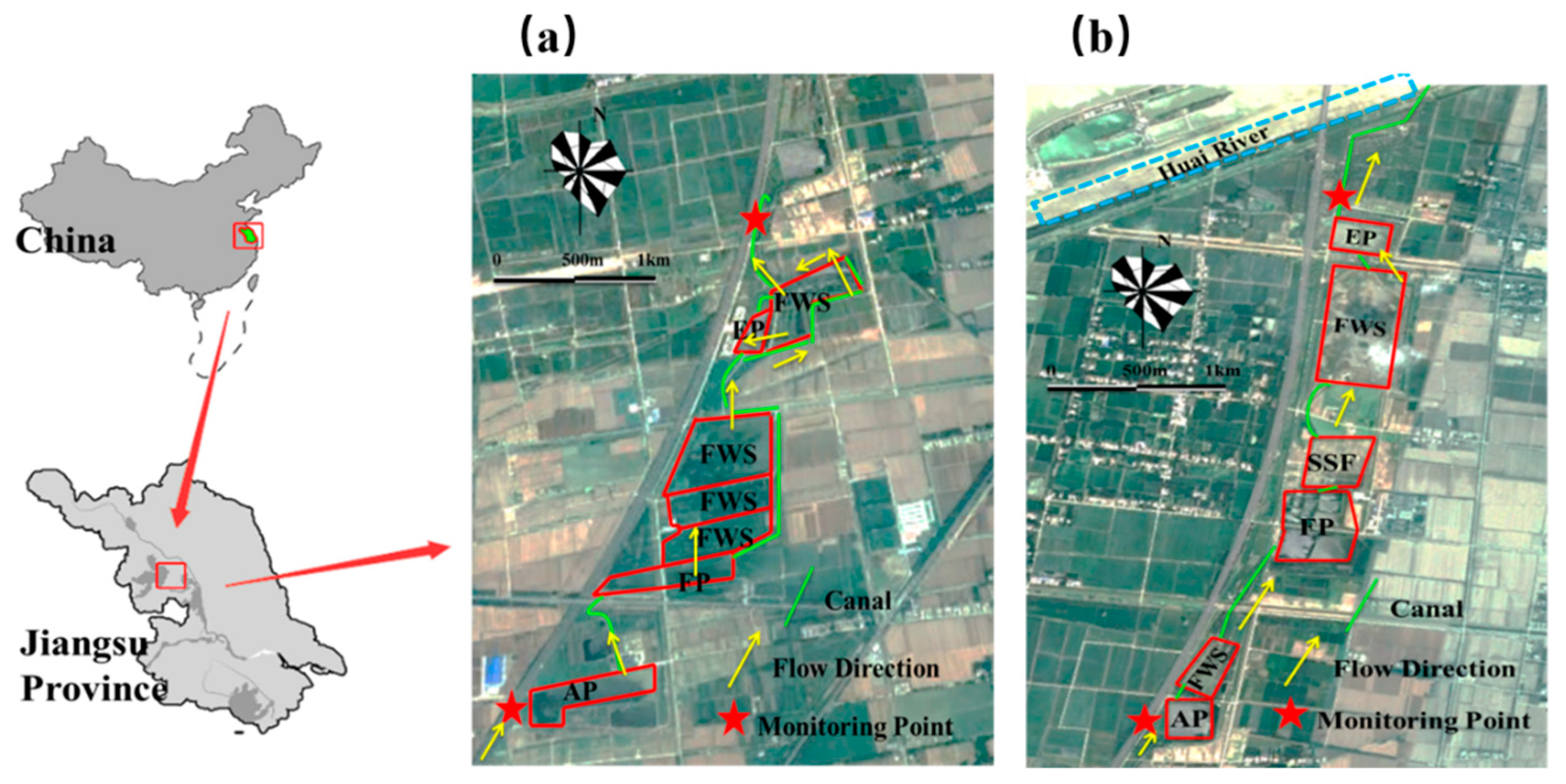
Both of the full-scale integrated CWs were situated in Hongze District, Jiangsu Province, East China (118°55′27″ E, 33°20′13″ N) (Figure 1), where the climate is subtropical with an annual average temperature of 14.9 °C and presents a clear distinction between the four seasons. The annual average precipitation is 913.3 mm [17,18].
The first CW system (named CW1 in the following text) possessed a designed wastewater treatment capacity of 40,000 m3·day−1, which is composed of an aeration pond (AP), a facultative pond (FP), a free water surface flow CW (FWS), an ecological pond (EP), and an ecological canal (ECs) with hydraulic retention times (HRTs) of 6.7, 4.1, 3.4, 2.5, and 0.22 days, respectively. The influent of CW1 was mainly the secondary effluent from a municipal STP. The other system (named CW2 in the following text) had a designed wastewater treatment capacity of 60,000 m3·day−1, which is composed of an AP, an FWS, a facultative pond (FP), a subsurface-flow CW (SSF), an EP, and ECs. The whole HRT of CW2 was 17.4 days. The influent of CW2 was mainly the secondary effluent from an industrial STP. More than 15 species of aquatic macrophytes were planted in CW1 and CW2, with Phragmites australis and Typha orientalis Presl as the dominant ones.
2.2. Online Water Quality Monitoring
The influent and effluent water quality parameters were measured using online water quality monitoring systems, termed Inf-CW1 and Inf-CW2 for the influents of CW1 and CW2, and Eff-CW1 and Eff-CW2 for the effluents of CW1 and CW2, respectively. The wastewater was pumped into auto-measurement systems for measurement of COD and NH4+-N, set up indoors with stable temperature, humidity, and lighting conditions. COD and NH4+-N were detected using the potassium dichromate method and Nessler reagent spectrophotometry method, respectively. The hourly sample interval was set for the influent and the effluent of CW1 and CW2. Due to the absence of data in December 2018, the data from December 2015 to November 2016, December 2016 to November 2017, and December 2017 to November 2018 were regarded as the data in 2016, 2017, and 2018, respectively.
2.3. Data Evaluation Method
It is known that the coefficient of variation is the ratio of the standard deviation of a set of data to the mean value, which can reflect the dispersion of these data. The calculation formula is as follows.
To evaluate the short-term temporal variability of COD and NH4+-N, one of the important factors influencing the SF, the modified coefficient of variation (CVm) was developed. Because the sample number (n) is two in each calculation, the equation can be simplified as follows:
where xt1 and xt2 are the measured COD or NH4+-N at times t1 and t2, respectively. The difference between t1 and t2 is the SI. To decrease the drastic fluctuation of the CV under conditions with very low COD or NH4+-N, a constant c was added. The constant c was calculated using 5% of the potential maximum COD or NH4+-N values. In this study, the constant c values were set to 5 mg/L and 2 mg/L for COD and NH4+-N, respectively.
To obtain the average or overall performance in a certain period, the variation rate (VR) was calculated to quantify the variation of the average COD or NH4+-N using a certain SI in a certain period from the average COD or NH4+-N using the hourly SI data. In this study, two types of VR were developed to evaluate the effect of SI on the estimation accuracy, i.e., the average variation rate at a certain SI (VRa) and the maximum variation rate at a certain SI (VRm), which were obtained from the calculated VR:
where is the average COD or NH4+-N of all the measured values in this study, i.e., the hourly SI data. The was the average COD or NH4+-N of a certain SI with the measured COD or NH4+-N at time t as the first value, i.e., one duplicate of a certain SI. For example, for the calculation of the average COD in 2018 at an SI of 10 h, there would be ten duplicates, i.e., the first measurements were at 0:00, 1:00, 2:00, 3:00, 4:00, 5:00, 6:00, 7:00, 8:00, and 9:00 on 1 January 2018, respectively. The VRa and VRm were the average values of the ten duplicates and the maximum VR in the ten duplicates, respectively.
3. Results and Discussion
3.1. The Average Value and Coefficient of Variation of COD and NH4+-N
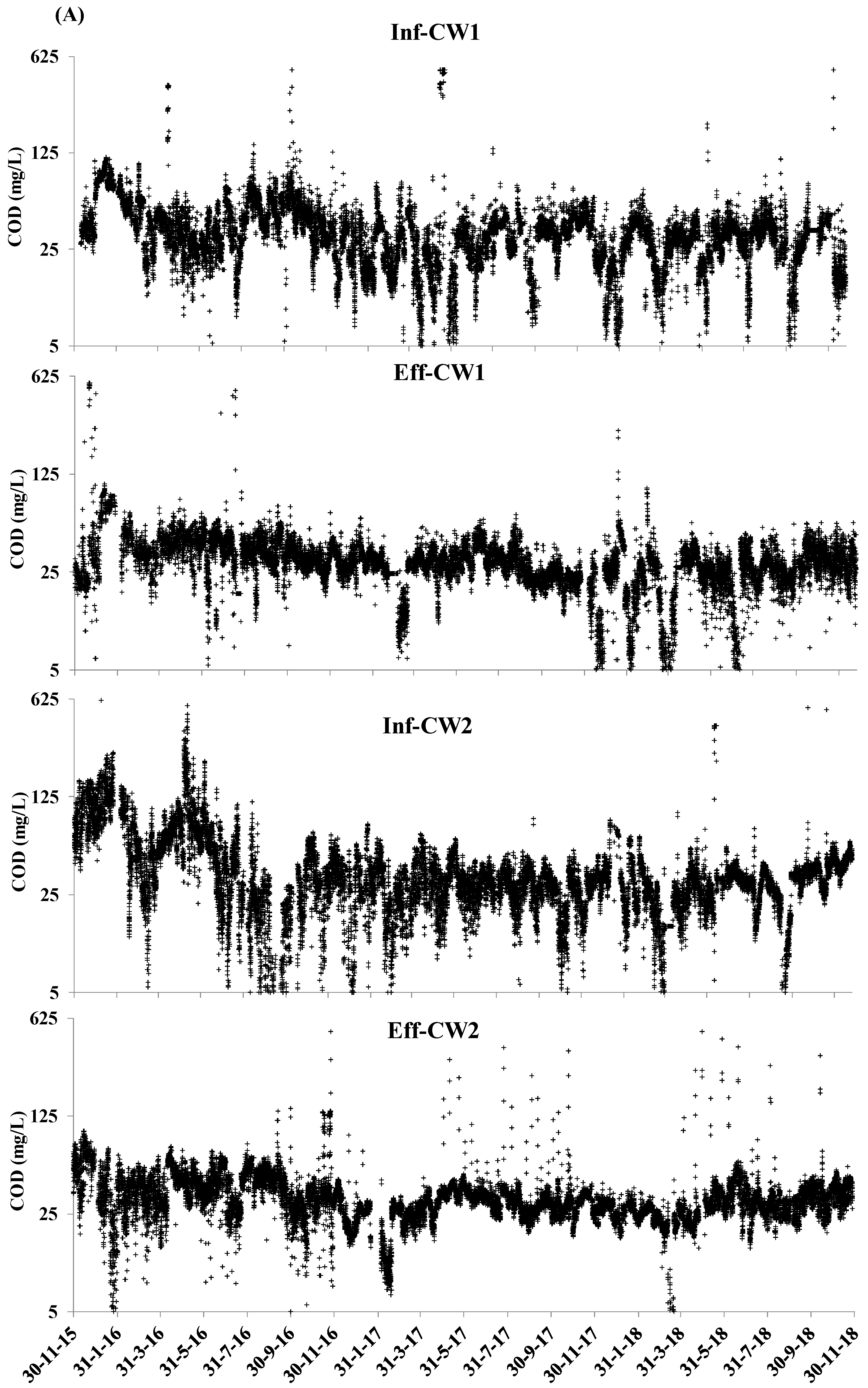
The statistics suggested that between 2016 and 2018, the average influent COD was 34.7 mg L−1 and 40.4 mg L−1, while the average effluent COD was 31.3 mg L−1 and 33.1 mg L−1 for CW1 and CW2, with REs of 10.0% and 18.1%, respectively (Table 1), which suggested that both CW1 and CW2 performed a slight removal of COD, probably related to the relatively low amount of readily biodegradable COD in the effluent wastewater from the STPs [19,20]. For CW1 and CW2, the NH4+-N RE was 61.8% and 71.5%, respectively, suggesting that both of the CWs showed a high removal of NH4+-N. The high NH4+-N RE is probably related to the relatively high dissolved oxygen concentration and long HRTs [17].
In the past three years, both COD and NH4+-N fluctuated in relatively large ranges in both the influent and the effluent of the two CWs (Figure 2), with an average CV value of 82.3% and 246.3% for COD and NH4+-N (Table 1), respectively. The fluctuation range was much larger than most of the published results of full-scale CWs from the literature [21,22,23]. The large fluctuation of COD and NH4+-N, on one hand, further proved the importance of SF in water quality monitoring for full-scale CWs; different SIs should be applied in both seasons and sampling sites for the monitoring of COD and NH4+-N in CWs. On the other hand, the measured water quality by automatic monitoring systems in both the influents and the effluents of full-scale CWs treating the wastewater from STPs probably fluctuated much more than expected. For large CWs, the seasonal average COD and NH4+-N, as well as their variation in the effluent, is probably determined by numerous factors, such as the temperature dependence of the purification function of the CW [23,24], the influent water quality, and the rainfall events, while the water quality of the influent from STPs was most was likely influenced by numerous factors, such as rainfall events, human activities related to wastewater discharge, and process choice selected by the STP.
3.2. The Suitable Sampling Frequency in Modified Coefficient of Variation
As expected, the CVm of NH4+-N and COD between two samplings significantly increased with the SI for all four sampling sites, which could be well modeled using either exponential or power functions, with R2 values of 0.998, 0.989, 0.991, 0.994, 0.990, 0.989, 0.985, and 0.991, respectively (Figure 3). For COD, when the SI increased from 2 h to 168 h, the average CVm gradually increased from 6.7% to 23.6%, from 5.6% to 16.9%, from 7.9% to 27.1%, and from 5.5% to 17.4% for Inf-CW1, Inf-CW2, Eff-CW1, and Eff-CW2, respectively. Therefore, in CVm, the COD for the four sites was relatively stable. However, the standard deviation (SD) values ranged from 11.6% to 23.1%, from 8.6% to 16.3%, from 10.6% to 25.1% and from 10.6% to 21.2%, with averages of 20.2%, 14.6%, 22.3%, and 18.3% for Inf-CW1, Inf-CW2, Eff-CW1, and Eff-CW2, respectively. For NH4+-N, similar results were observed, i.e., the average CVm ranged from 5.0% to 27.2%, from 3.7% to 13.8%, from 3.5% to 21.0%, and from 6.2% to 18.4% for Inf-CW1, Inf-CW2, Eff-CW1, and Eff-CW2, respectively. However, the average SD of NH4+-N ranged from 20.2% to 28.8% for the four sampling sites. For the widely used daily and weekly SF, the variation rates in CVm were 13.0% and 19.8% for COD and 14.0% and 20.7% for NH4+-N, respectively. In addition, the relatively large SD values showed large temporal fluctuation in both COD and NH4+-N, which suggested that there were large uncertainties in studying the temporal dynamics of COD or NH4+-N without high SF data. The current widely used SF is not sufficient for studying the dynamics of water quality for secondary CW.
At 5%, 10%, and 15% CVm, the SIs were statistically analyzed (Table 2). For the overall data of the three years, the SIs ranged from 0.2 to 1.7 h, 3.4 to 17.8 h, and 16.0 to 92.3 h for COD at 5%, 10%, and 15% CVm, respectively; additionally, for NH4+-N, the SIs ranged from 1.7 to 5.3 h, from 6.6 to 35.1 h, and from 16.3 to 291.6 h at 5%, 10%, and 15% CVm, respectively. At 10%, the average SIs were 9.8, 16.6, 12.9, and 9.9 h for COD in spring, summer, autumn, and winter, respectively; for NH4+-N, the values were 18.2, 44.8, 64.2, and 10.1 h in spring, summer, autumn, and winter, respectively. Therefore, between seasons, both COD and NH4+-N were generally stable and thus allowed relatively larger SIs in summer and autumn; in contrast, COD and NH4+-N varied more drastically and thus allowed relatively smaller SIs in winter. Between sampling sites, the effluent COD and NH4+-N had larger SIs than that in the influent for both CW1 and CW2 in the same CVm standard, with the exceptions of NH4+-N in CW2 at 5% and 10% CVm. The results suggested that, at 5%, 10%, and 15% acceptable variation in CVm, the average SIs were 1.19, 11.92, and 80.53 h for COD and 4.51, 30.73, and 192.24 h for NH4+-N, respectively. Generally, there requires a higher SF in winter than that in summer or autumn and a higher SF in the influent than that in the effluent.
Temporal variability is one of the dominant factors influencing the SF [16]. The parameter CVm is probably not suitable for evaluating the overall performance of a CW in a certain period [9,25]. However, if the main purpose of monitoring is focused on the detailed process as well as the driving factors of the CW purification function, CVm is probably a robust parameter that can quantify the temporal variation rate of water quality. Considering the inevitable error in the process of chemical analysis (or measurement instrument) and sampling, the 10–15% CVm is probably more acceptable than the 5% standard for most cases in determining the proper SF, at which the suitable SI for the secondary CW ranged from the half-days to the weekly. However, the relatively large SD values suggested that, at such SIs, some detailed process information will be inevitably lost for secondary CWs, which is consistent with the results of previous studies [9].
The water quality variation in the influent from the STP is influenced by the factors related to the STP operation performance, the artificial adjustment, and the wastewater discharged to the STP, which differs from polluted rivers and lakes [16,26]; thus, the variation characteristics of the influent water quality are different between the CW treating the secondary effluent from the STP and the CW treating other polluted water. Compared with the influent from polluted rivers or lakes, our results suggested that the influent from the STP varied more rapidly [10,16,23]. In this study, the influents of CW1 and CW2 were from the secondary STPs treating industrial and municipal wastewater, respectively. The difference in the source of the wastewater could also result in the difference in the water quality variation between CW1 and CW2. Our results suggested that the influent water quality variation rate of CW1 was more rapid than that of CW2.
The water quality variation rate of the effluent was mainly determined by the influent characteristic and the purification function of the CW. A linear relationship generally exists between the influent and effluent water quality of CWs [6,27], which can be weakened by the buffering function of CWs, especially for full-scale CWs [28]. The short-term fluctuation of the CW purification function is determined by the microbial activity, plant growth rate, and residue decomposition, which are related to environmental factors such as temperature. The diurnal and irregular fluctuation of temperature influences the effluent water quality fluctuation [29,30], which can also be weakened by the buffering function of the CW. Our result, i.e., the generally larger variation rate of the effluent water quality than that of the influent, can be explained by the buffering function of the CW [28], which is different from the CW treating the polluted river water [7].
3.3. The Proper Sampling Interval in Average Variation Rate and the Maximum Variation Rate
3.3.1. Average Variation Rate (VRa)
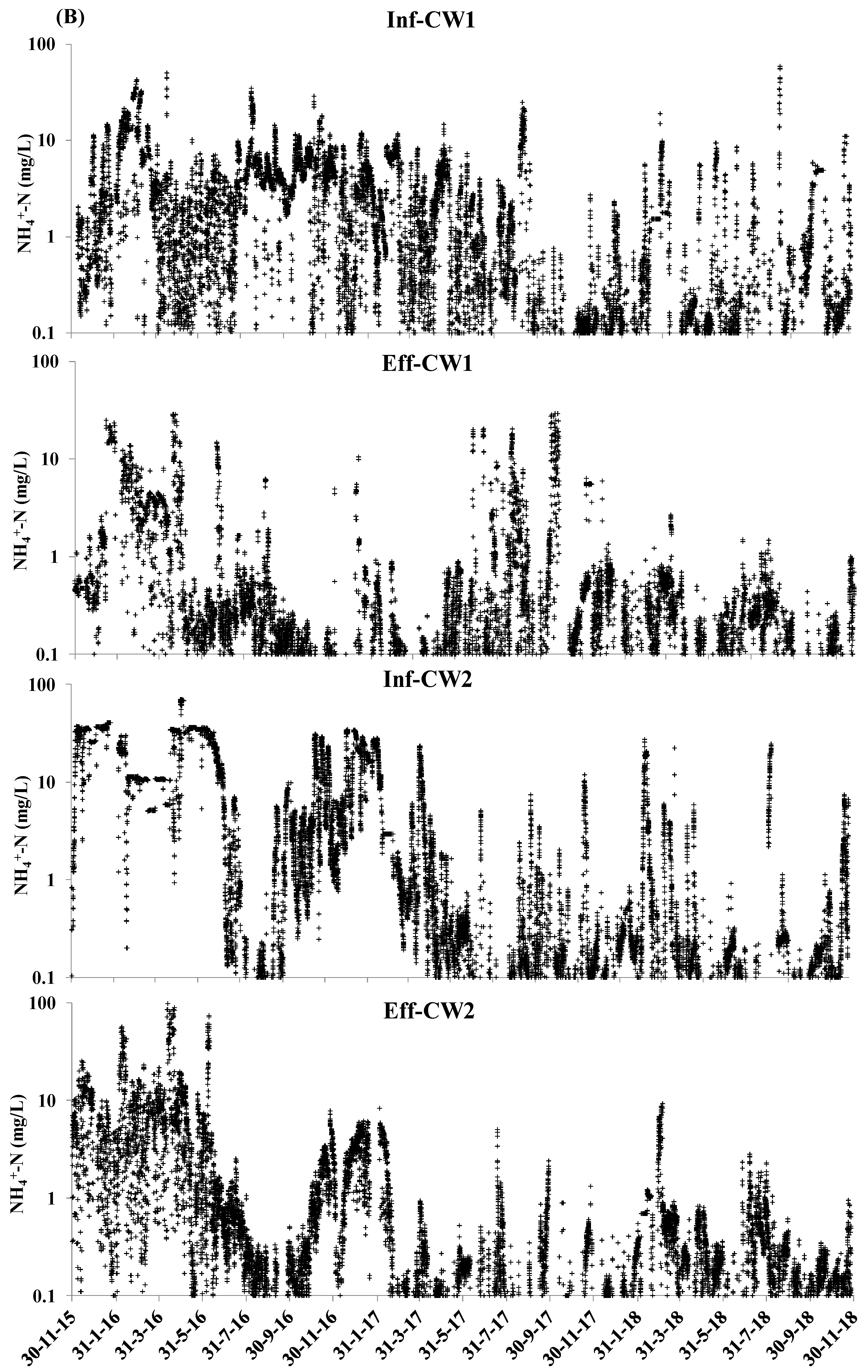
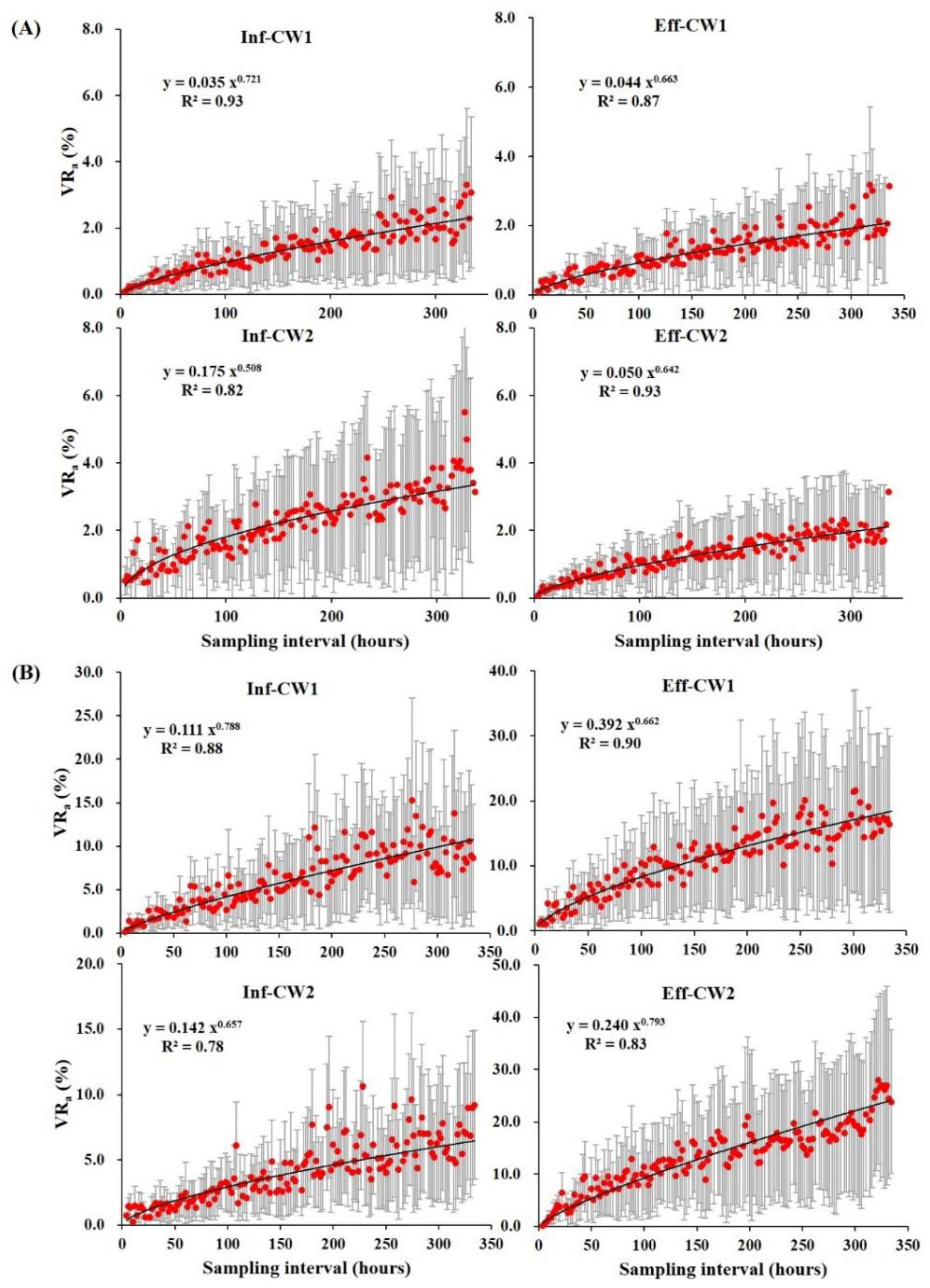
As expected, significant relationships were observed between the VRa values and the SIs for both COD and NH4+-N, which could be well modeled using power functions, with R2 values ranging from 0.82 to 0.93 and 0.79 to 0.90, respectively (Figure 4). When the SIs fluctuated between 2 h and 334 h, 1.37%, 1.29%, 2.30%, and 1.31% average VRa values in COD and 6.18%, 11.2%, 4.12%, and 13.39% in NH4+-N were observed for Inf-CW1, Inf-CW2, Eff-CW1, and Eff-CW2, respectively. According to the power models, the VRa value at a certain SI could be quantified. For example, at SIs of 1, 7, and 14 days, an average VRa of 0.49%, 1.61%, and 2.46% in COD and an average VRa of 2.18%, 9.01%, and 15.00% in NH4+-N was observed at the four sites, respectively. The results suggested that, for COD, increasing the SI from 2 h to 2 weeks only slightly decreased the monitoring accuracy in VRa, while for NH4+-N, the monitoring accuracy substantially decreased. For NH4+-N, the estimation accuracy had only a slight decrease when the SI increased from 1 h to 1 day. Therefore, in VRa, the daily SI was suitable for monitoring the average performance of COD and NH4+-N.
At the 5%, and 10% variation rates in VRa, the SIs were statistically analyzed (Table 3). For COD, an average of 526.5, and 1401.7 h of SI were obtained for the four sites at the VRa of 5% and 10%, respectively. For NH4+-N, at VRa values of 5% and 10%, ranges from 10.8 to 200.9 h and from 28.4 to 421.8 h were obtained, respectively, with an average of 66.3 and 139.3 h of SI. The results suggested that, at a 5% acceptable error in VRa, the average SI was 526.5 and 66.3 h for COD and NH4+-N, respectively. Therefore, in VRa, the weekly and daily SI were suitable for monitoring the annual average COD and NH4+-N, respectively.
3.3.2. The Maximum Average Variation Rate (VRm)
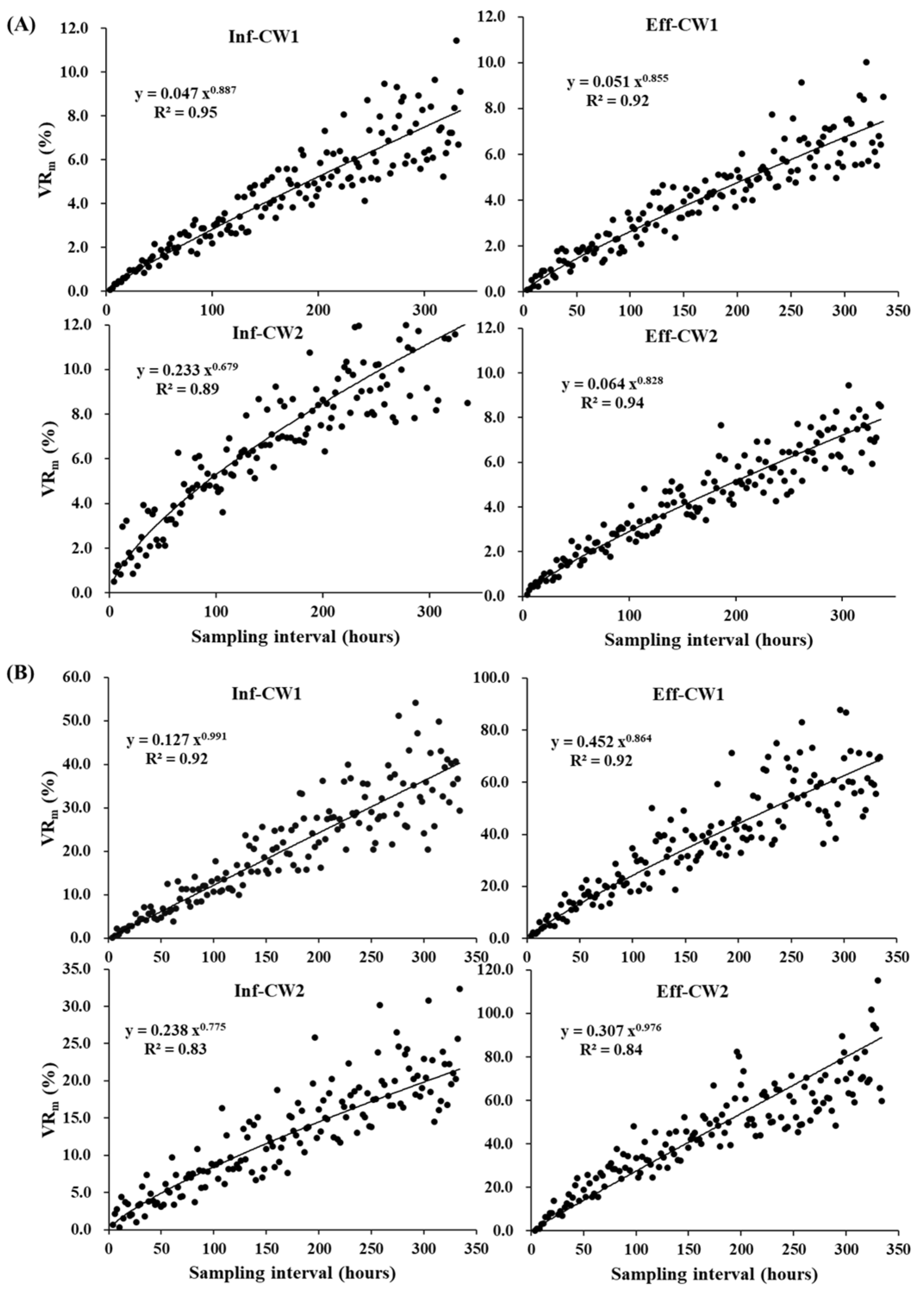
In Figure 4, the SD values were relatively large, i.e., the average SD values were 1.14% and 6.31% for COD and NH4+-N, respectively. Therefore, to be safe, we also analyzed the proper SI using the stricter parameter of the VRm value (Figure 5). Significant relationships were observed between the SI and VRm values for both COD and NH4+-N at the four sites, with R2 values of 0.95, 0.92, 0.89, 0.94, 0.92, 0.92, 0.83, and 0.84, respectively. Compared with VRa, the VRm value greatly increased at the same SI. With the SI fluctuating between 2 and 334 h, the average VRm values for the four sites were 5.09% and 29.00% for COD and NH4+-N, respectively. In the VRm value, weekly and daily were the suitable SIs for the calculation of the annual average values for COD and NH4+-N, respectively, which could obtain an average estimation accuracy of 5.13% and 4.91% for COD and NH4+-N, respectively.
For COD, at the acceptable errors of 5% and 10% in VRm, the SI ranges of 53.8–163.9 and 123.6–361.6 h were obtained, respectively, with an average SI of 110.1 and 233.5 h, respectively (Table 4). For NH4+-N, SI ranges of 6.1–70.0 and 12.4–134.4 h were obtained for the acceptable errors of 5%, and 10% in VRm, respectively, with an average of 26.8 and 50.5 h, respectively. Generally, NH4+-N required a lower SI than did COD. At the acceptable error of 5% in VRm, the average SF was 110.1 and 26.8 h, respectively. Therefore, four-day and one-day SIs were suitable for the evaluation of the annual performance of the COD and NH4+-N, respectively.
In contrast to CVm, the parameter VRm (or VRa) at the annual scale generally experiences a relatively lower influence by the periodic variation in water quality, such as the variation related to the diurnal and seasonal variation in temperature. However, the SF should be high enough to obtain information on the short-term and strong fluctuation of water quality related to events such as storms and snow melting [9,10]. To decrease the direct effect of the toxic secondary effluent from STPs on human health, secondary CWs are generally built in areas isolated from residential communities; thus, water quality is seldom directly influenced by irregular human activity, such as the discharge of untreated polluted water. The catchment function of the secondary CW also decreases by building isolated rivers along with the secondary CW that prevent the outflow of the toxic secondary water, which can greatly decrease the effect of short-term and strong events, such as storms and snow melting [9,26,31]. These characteristics of the secondary CW can greatly decrease the short-term fluctuation of water quality in CWs and thus potentially decrease the SF requirement.
However, there are some factors that can increase the fluctuation of water quality and thus the SF demand. In CW, the relatively large biomass of aquatic macrophytes can induce the short-term strong fluctuation of water quality, especially at the early decomposition stage of the dead residue [18]. In addition, compared with polluted rivers or lakes, the water quality of the influent directly from the STP fluctuates more than that of the polluted rivers or lakes due to the buffering of rivers or lakes [10,16,23]. Therefore, the SF of the secondary CW must be high enough to obtain information about the short-term and probably strong fluctuations in water quality caused by these factors. As an alternative, instead of a constant SF, real-time adaptive sampling controlled by trigger variables may be more efficient because it balances the obtainment of the hot moments of nutrient dynamics and reduces data redundancy [26]. In future work, the suitability of the adaptive sampling strategy needs to be identified in secondary CWs.
4. Conclusions
The suitable sampling frequency was quantified at the acceptable errors of 5% and 10%. At 5% of CVm, the average SIs were 1.1 h and 4 h for COD and NH4+-N. At 10% of CVm, the average SIs were 11.92 and 30.73 h for COD and NH4+-N, respectively. At 5% of VRa, the average SIs were 526.5 and 66.3 h for COD and NH4+-N, respectively. At 5% VRm, the average SIs were 110.1 and 26.8 h for COD and NH4+-N, respectively. Therefore, to meet the needs of monitoring the dynamic change of data and annual effect evaluation at the same time, hourly and 4 h SI were recommended for COD and NH4+-N evaluation, respectively, when strict requirements are required; when it is necessary to consider the operation and maintenance costs at the same time, 11 h and 30 h SIs were proper for COD and NH4+-N evaluation, respectively. This research developed the methods for quantifying the suitable sampling frequency in the dynamic monitoring and average performance evaluation and also identified the relationship between sampling frequency and monitoring error for the dynamic analysis and average performance evaluation in specific periods, which could be promoted to other full-scale CWs.
Author Contributions
Conceptualization, S.S. (Sheng Sheng) and D.Z.; data curation, S.S. (Siyuan Song) and J.X.; formal analysis, S.S. (Siyuan Song); writing—original draft, S.S. (Siyuan Song); writing—review and editing, S.S. (Siyuan Song), S.S. (Sheng Sheng) and D.Z. All authors have read and agreed to the published version of the manuscript.
Funding
This research was funded by Zhejiang Province Postdoctoral Research Funding Project (No. ZJ2021047).
Institutional Review Board Statement
Not applicable.
Informed Consent Statement
Not applicable.
Data Availability Statement
Not applicable.
Acknowledgments
The authors declare no conflict of interest.
Conflicts of Interest
The authors declare no conflict of interest. The funders had no role in the design of the study; in the collection, analyses, or interpretation of data; in the writing of the manuscript, or in the decision to publish the results.
References
- Ji, M.; Hu, Z.; Hou, C.; Liu, H.; Ngo, H.H.; Guo, W.; Lu, S.; Zhang, J. New insights for enhancing the performance of constructed wetlands at low temperatures. Bioresour. Technol. 2020, 301, 122722. [Google Scholar] [CrossRef] [PubMed]
- Ali, M.; Rousseau, D.P.L.; Ahmed, S. A full-scale comparison of two hybrid constructed wetlands treating domestic wastewater in Pakistan. J. Environ. Manag. 2018, 210, 349–358. [Google Scholar] [CrossRef] [PubMed]
- Liu, Y.; Engel, B.A.; Flanagan, D.C.; Gitau, M.W.; McMillan, S.K.; Chaubey, I. A review on effectiveness of best management practices in improving hydrology and water quality: Needs and opportunities. Sci. Total Environ. 2017, 601–602, 580–593. [Google Scholar] [CrossRef] [PubMed]
- Matamoros, V.; Rodriguez, Y.; Bayona, J.M. Mitigation of emerging contaminants by full-scale horizontal flow constructed wetlands fed with secondary treated wastewater. Ecol. Eng. 2017, 99, 222–227. [Google Scholar] [CrossRef]
- Pelissari, C.; Ávila, C.; Trein, C.M.; García, J.; de Armas, R.D.; Sezerino, P.H. Nitrogen transforming bacteria within a full-scale partially saturated vertical subsurface flow constructed wetland treating urban wastewater. Sci. Total Environ. 2017, 574, 390–399. [Google Scholar] [CrossRef] [Green Version]
- Wu, H.; Fan, J.; Zhang, J.; Ngo, H.H.; Guo, W. Large-scale multi-stage constructed wetlands for secondary effluents treatment in northern China: Carbon dynamics. Environ. Pollut. 2018, 233, 933–942. [Google Scholar] [CrossRef] [Green Version]
- Drake, C.; Jones, C.; Schilling, K.; Amado, A.A.; Weber, L. Estimating nitrate-nitrogen retention in a large constructed wetland using high-frequency, continuous monitoring and hydrologic modeling. Ecol. Eng. 2018, 117, 69–83. [Google Scholar] [CrossRef]
- Rode, M.; Wade, A.J.; Cohen, M.J.; Hensley, R.; Bowes, M.; Kirchner, J.W.; Arhonditsis, G.; Jordan, P.; Kronvang, B.; Halliday, S.; et al. Sensors in the Stream: The High-Frequency Wave of the Present. Environ. Sci. Technol. 2016, 50, 10297–10307. [Google Scholar] [CrossRef] [Green Version]
- Valkama, P.; Mäkinen, E.; Ojala, A.; Vahtera, H.; Lahti, K.; Rantakokko, K.; Vasander, H.; Nikinmaa, E.; Wahlroos, O. Seasonal variation in nutrient removal efficiency of a boreal wetland detected by high-frequency on-line monitoring. Ecol. Eng. 2017, 98, 307–317. [Google Scholar] [CrossRef]
- Chappell, N.A.; Jones, T.D.; Tych, W. Sampling frequency for water quality variables in streams: Systems analysis to quantify minimum monitoring rates. Water Res. 2017, 123, 49–57. [Google Scholar] [CrossRef]
- Zhao, D.; Cai, Y.; Jiang, H.; Xu, D.; Zhang, W.; An, S. Estimation of water clarity in Taihu Lake and surrounding rivers using Landsat imagery. Adv. Water Resour. 2011, 34, 165–173. [Google Scholar] [CrossRef]
- Brauer, N.; O’Geen, A.T.; Dahlgren, R.A. Temporal variability in water quality of agricultural tailwaters: Implications for water quality monitoring. Agric. Water Manag. 2009, 96, 1001–1009. [Google Scholar] [CrossRef]
- Jones, A.S.; Horsburgh, J.S.; Mesner, N.O.; Ryel, R.J.; Stevens, D.K. Influence of sampling frequency on estimation of annual total phosphorus and total suspended solids loads. J. Am. Water Resour. Assoc. 2012, 48, 1258–1275. [Google Scholar] [CrossRef]
- Andreo-Martínez, P.; García-Martínez, N.; Quesada-Medina, J.; Almela, L. Domestic wastewaters reuse reclaimed by an improved horizontal subsurface-flow constructed wetland: A case study in the southeast of Spain. Bioresour. Technol. 2017, 233, 236–246. [Google Scholar] [CrossRef]
- Ávila, C.; Salas, J.J.; Martín, I.; Aragón, C.; García, J. Integrated treatment of combined sewer wastewater and stormwater in a hybrid constructed wetland system in southern Spain and its further reuse. Ecol. Eng. 2013, 50, 13–20. [Google Scholar] [CrossRef]
- Vilmin, L.; Flipo, N.; Escoffier, N.; Groleau, A. Estimation of the water quality of a large urbanized river as defined by the European WFD: What is the optimal sampling frequency? Environ. Sci. Pollut. Res. 2018, 25, 23485–23501. [Google Scholar] [CrossRef] [Green Version]
- Song, S.; Liu, B.; Zhang, W.; Wang, P.; Qiao, Y.; Zhao, D.; Yang, T.; An, S.; Leng, X. Performance of a large-scale wetland treatment system in treating tailwater from a sewage treatment plant. Mar. Freshw. Res. 2018, 69, 833–841. [Google Scholar] [CrossRef]
- Zhao, D.; Zhang, M.; Liu, Z.; Sheng, J.; An, S. Can cold-season macrophytes at the senescence stage improve nitrogen removal in integrated constructed wetland systems treating low carbon/nitrogen effluent? Bioresour. Technol. 2018, 265, 380–386. [Google Scholar] [CrossRef]
- Chen, Y.; Wen, Y.; Zhou, Q.; Vymazal, J. Effects of plant biomass on nitrogen transformation in subsurface-batch constructed wetlands: A stable isotope and mass balance assessment. Water Res. 2014, 63, 158–167. [Google Scholar] [CrossRef]
- Zhang, C.; Yin, Q.; Wen, Y.; Guo, W.; Liu, C.; Zhou, Q. Enhanced nitrate removal in self-supplying carbon source constructed wetlands treating secondary effluent: The roles of plants and plant fermentation broth. Ecol. Eng. 2016, 91, 310–316. [Google Scholar] [CrossRef] [Green Version]
- Dunne, E.J.; Coveney, M.F.; Marzolf, E.R.; Hoge, V.R.; Conrow, R.; Naleway, R.; Lowe, E.F.; Battoe, L.E.; Inglett, P.W. Nitrogen dynamics of a large-scale constructed wetland used to remove excess nitrogen from eutrophic lake water. Ecol. Eng. 2013, 61, 224–234. [Google Scholar] [CrossRef]
- Tilley, D.R.; Badrinarayanan, H.; Rosati, R.; Son, J. Constructed wetlands as recirculation filters in large-scale shrimp aquaculture. Aquac. Eng. 2002, 26, 81–109. [Google Scholar] [CrossRef]
- Wu, H.; Zhang, J.; Guo, W.; Liang, S.; Fan, J. Secondary effluent purification by a large-scale multi-stage surface-flow constructed wetland: A case study in northern China. Bioresour. Technol. 2018, 249, 1092–1096. [Google Scholar] [CrossRef] [PubMed]
- Jóźwiakowski, K.; Bugajski, P.; Kurek, K.; Cáceres, R.; Siwiec, T.; Jucherski, A.; Czekała, W.; Kozłowski, K. Technological reliability of pollutant removal in different seasons in one-stage constructed wetland system with horizontal flow operating in the moderate climate. Sep. Purif. Technol. 2020, 238, 116439. [Google Scholar] [CrossRef]
- Wu, S.; Wallace, S.; Brix, H.; Kuschk, P.; Kirui, W.K.; Masi, F.; Dong, R. Treatment of industrial effluents in constructed wetlands: Challenges, operational strategies and overall performance. Environ. Pollut. 2015, 201, 107–120. [Google Scholar] [CrossRef]
- Blaen, P.J.; Khamis, K.; Lloyd, C.E.; Bradley, C.; Hannah, D.; Krause, S. Real-time monitoring of nutrients and dissolved organic matter in rivers: Capturing event dynamics, technological opportunities and future directions. Sci. Total Environ. 2016, 569–570, 647–660. [Google Scholar] [CrossRef] [Green Version]
- Rizzo, A.; Langergraber, G. Novel insights on the response of horizontal flow constructed wetlands to sudden changes of influent organic load: A modeling study. Ecol. Eng. 2016, 93, 242–249. [Google Scholar] [CrossRef]
- Galvao, A.; Matos, J. Response of horizontal sub-surface flow constructed wetlands to sudden organic load changes. Ecol. Eng. 2012, 49, 123–129. [Google Scholar] [CrossRef]
- García, J.; Green, B.; Lundquist, T.; Mujeriego, R.; Hernández-Mariné, M.; Oswald, W. Long term diurnal variations in contaminant removal in high rate ponds treating urban wastewater. Bioresour. Technol. 2006, 97, 1709–1715. [Google Scholar] [CrossRef]
- Kahl, S.; Nivala, J.; van Afferden, M.; Müller, R.A.; Reemtsma, T. Effect of design and operational conditions on the performance of subsurface flow treatment wetlands: Emerging organic contaminants as indicators. Water Res. 2017, 125, 490–500. [Google Scholar] [CrossRef]
- Fauvel, B.; Cauchie, H.-M.; Gantzer, C.; Ogorzaly, L. Contribution of hydrological data to the understanding of the spatio-temporal dynamics of F-specific RNA bacteriophages in river water during rainfall-runoff events. Water Res. 2016, 94, 328–340. [Google Scholar] [CrossRef] [PubMed]
Figure 1.
Geographic location and layout of (a) CW1 and (b) CW2 (AP, aerated pond; FP, facultative pond; FWS, free water surface flow constructed wetland; EP, ecological pond; SSF, subsurface flow constructed wetland).
Figure 1.
Geographic location and layout of (a) CW1 and (b) CW2 (AP, aerated pond; FP, facultative pond; FWS, free water surface flow constructed wetland; EP, ecological pond; SSF, subsurface flow constructed wetland).

Figure 2.
The temporal dynamics of the measured COD (A) and NH4+-N (B) from 10 November 2015 to 28 November 2018 (n = 26,038). A logarithmic scale was used for the y-axis to improve the discrimination between samplings with values concentrated over relatively narrow regions (relatively low regions). The symbol “+” represents a data.


Figure 3.
The relationships between the sampling interval (SI) and the variation between the two sampling times in the modified coefficient of variation (CVm) for monitoring the temporal dynamics of COD (A) and NH4+-N (B) (n = 26,038). R2 values represent the coefficient of determination of the exponential or power model between the SI and CVm for monitoring the temporal dynamics of COD and NH4+-N.

Figure 4.
The relationships between the sampling intervals (SIs) and the average variation rates (VRa) for the evaluation of the three-year average performance of COD (A) and NH4+-N (B) between 10 November 2015 and 28 November 2018. R2 values represent the coefficient of determination of the power model between the SIs and VRa for the evaluation of the three-year average performance of COD and NH4+-N.

Figure 5.
The relationships between the SF and the maximum variation rate (VRm) in COD (A) and NH4+-N (B) using all the data from 2016 to 2018 with the hourly SF data.
Figure 5.
The relationships between the SF and the maximum variation rate (VRm) in COD (A) and NH4+-N (B) using all the data from 2016 to 2018 with the hourly SF data.


Table 1.
The average value and the coefficient of variation of COD and NH4+-N in the influent and effluent water.
Table 1.
The average value and the coefficient of variation of COD and NH4+-N in the influent and effluent water.
| Site | COD | NH4+-N | ||
|---|---|---|---|---|
| Mean (mg L−1) | CV (%) | Mean (mg L−1) | CV (%) | |
| Inf-CW1 | 34.7 | 82.3 | 2.41 | 182.9 |
| Eff-CW1 | 31.3 | 100.6 | 0.92 | 302.2 |
| Inf-CW2 | 40.4 | 100.0 | 6.21 | 183.9 |
| Eff-CW2 | 33.1 | 46.1 | 1.83 | 316.0 |
Table 2.
The average SI (h) for the acceptable CVm values of 5%, 10%, and 15%.
| Site | Season | COD | NH4+-N | ||||
|---|---|---|---|---|---|---|---|
| 5% | 10% | 15% | 5% | 10% | 15% | ||
| Inf-CW1 | Spring | 0.3 | 4.0 | 17.8 | 1.3 | 3.3 | 8.2 |
| Summer | 1.4 | 13.6 | 51.9 | 3.0 | 8.0 | 21.5 | |
| Autumn | 1.1 | 12.7 | 53.7 | 4.3 | 12.8 | 38.2 | |
| Winter | 0.9 | 8.3 | 29.8 | 3.6 | 6.9 | 13.5 | |
| Overall | 0.8 | 8.4 | 33.9 | 2.7 | 6.6 | 16.3 | |
| Eff-CW1 | Spring | 1.1 | 8.9 | 72.6 | 4.2 | 50.6 | 611.4 |
| Summer | 1.0 | 11.2 | 121.3 | 2.9 | 17.1 | 100.4 | |
| Autumn | 1.4 | 24.4 | 413.5 | 22.1 | 204.0 | 748.0 | |
| Winter | 1.3 | 12.4 | 47.3 | 2.9 | 15.9 | 86.0 | |
| Overall | 1.7 | 12.2 | 89.0 | 4.2 | 35.1 | 291.6 | |
| Inf-CW2 | Spring | 1.4 | 4.7 | 15.9 | 4.6 | 12.7 | 35.4 |
| Summer | 1.1 | 12.7 | 53.7 | 10.5 | 88.4 | 744.8 | |
| Autumn | 0.4 | 4.9 | 21.2 | 4.0 | 9.2 | 21.0 | |
| Winter | 1.8 | 4.1 | 9.5 | 3.6 | 15.0 | 34.2 | |
| Overall | 0.2 | 3.4 | 16.0 | 5.3 | 14.7 | 40.7 | |
| Eff-CW2 | Spring | 2.2 | 21.6 | 81.7 | 1.5 | 6.2 | 26.5 |
| Summer | 3.4 | 28.8 | 247.4 | 5.5 | 65.5 | 775.6 | |
| Autumn | 0.3 | 9.6 | 66.6 | 1.6 | 30.6 | 170.6 | |
| Winter | 0.9 | 14.6 | 75.5 | 0.7 | 2.5 | 8.1 | |
| Overall | 1.1 | 17.8 | 92.3 | 1.7 | 9.4 | 52.8 | |
Table 3.
The average SF (h) for the average variation rate (VRa) values of 5% and 10%.
| Site | COD | NH4+-N | |||
|---|---|---|---|---|---|
| 5% | 10% | 5% | 10% | ||
| Inf-CW1 | 2018 | 450.0 | 1124.3 | 21.6 | 51.1 |
| 2017 | 342.7 | 811.4 | 94.7 | 179.8 | |
| 2016 | 427.4 | 1019.9 | 102.8 | 193.9 | |
| Eff-CW1 | 2018 | 379.5 | 1083.7 | 44.4 | 88.5 |
| 2017 | 817.6 | 2234.8 | 10.8 | 28.4 | |
| 2016 | 451.4 | 1020.3 | 53.9 | 129.4 | |
| Inf-CW2 | 2018 | 459.9 | 1131.7 | 30.5 | 63.1 |
| 2017 | 261.6 | 530.1 | 96.2 | 177.3 | |
| 2016 | 232.1 | 665.8 | 200.9 | 421.8 | |
| Eff-CW2 | 2018 | 822.1 | 2175.4 | 34.7 | 84.7 |
| 2017 | 1255.6 | 3753.9 | 62.9 | 160.7 | |
| 2016 | 417.9 | 1269.3 | 41.8 | 92.3 | |
Table 4.
The average SF (h) for the maximum variation rate (VRm) values of 5% and 10%.
| Site | COD | NH4+-N | |||
|---|---|---|---|---|---|
| 5% | 10% | 5% | 10% | ||
| Inf-CW1 | 2018 | 107.0 | 215.2 | 11.6 | 20.8 |
| 2017 | 88.4 | 179.2 | 40.8 | 72.4 | |
| 2016 | 108.9 | 221.3 | 44.3 | 76.0 | |
| Eff-CW1 | 2018 | 79.7 | 181.3 | 20.7 | 39.3 |
| 2017 | 161.6 | 357.0 | 6.1 | 12.4 | |
| 2016 | 125.0 | 248.8 | 19.3 | 40.2 | |
| Inf-CW2 | 2018 | 109.7 | 228.8 | 12.0 | 23.0 |
| 2017 | 91.6 | 171.4 | 42.7 | 77.2 | |
| 2016 | 53.8 | 123.6 | 70.0 | 134.4 | |
| Eff-CW2 | 2018 | 156.1 | 338.1 | 14.8 | 30.6 |
| 2017 | 163.9 | 361.6 | 21.5 | 45.5 | |
| 2016 | 75.3 | 175.3 | 18.2 | 34.5 | |
Publisher’s Note: MDPI stays neutral with regard to jurisdictional claims in published maps and institutional affiliations. |
© 2022 by the authors. Licensee MDPI, Basel, Switzerland. This article is an open access article distributed under the terms and conditions of the Creative Commons Attribution (CC BY) license (https://creativecommons.org/licenses/by/4.0/).
Share and Cite
MDPI and ACS Style
Song, S.; Sheng, S.; Xu, J.; Zhao, D. What Is the Suitable Sampling Frequency for Water Quality Monitoring in Full-Scale Constructed Wetlands Treating Tail Water? Water 2022, 14, 2431. https://doi.org/10.3390/w14152431
AMA Style
Song S, Sheng S, Xu J, Zhao D. What Is the Suitable Sampling Frequency for Water Quality Monitoring in Full-Scale Constructed Wetlands Treating Tail Water? Water. 2022; 14(15):2431. https://doi.org/10.3390/w14152431
Chicago/Turabian StyleSong, Siyuan, Sheng Sheng, Jianqiang Xu, and Dehua Zhao. 2022. "What Is the Suitable Sampling Frequency for Water Quality Monitoring in Full-Scale Constructed Wetlands Treating Tail Water?" Water 14, no. 15: 2431. https://doi.org/10.3390/w14152431
Note that from the first issue of 2016, this journal uses article numbers instead of page numbers. See further details here.