
The Setpoint Curve as a Tool for the Energy and Cost Optimization of Pumping Systems in Water Networks
by
 , , and
Christian F. León-Celi
1 ,
,
Pedro L. Iglesias-Rey
2,
Francisco Javier Martínez-Solano
2 and
and
Daniel Mora-Melia
3,* 1
Departamento de Ingeniería Ambiental, Facultad de Agropecuaria y Recursos Naturales, Universidad Nacional de Loja, Avenida Pio Jaramillo Alvarado, Loja 110103, Ecuador
2
Department of Hydraulic Engineering and Environment, Universitat Politècnica de València (Valencia Tech), 46022 Valencia, Spain
3
Departamento de Ingeniería y Gestión de la Construcción, Facultad de Ingeniería, Universidad de Talca, Camino Los Niches km.1, Curicó 3340000, Chile
*
Author to whom correspondence should be addressed.
Water 2022, 14(15), 2426; https://doi.org/10.3390/w14152426
Submission received: 13 June 2022
/
Revised: 28 July 2022
/
Accepted: 29 July 2022
/
Published: 5 August 2022
(This article belongs to the Section Urban Water Management)
Abstract
:In water distribution networks, the adjustment of the driving curves of pumping systems to the setpoint curves allows for determining the minimum energy cost that can be achieved in terms of pumping. This paper presents the methodology for calculating the optimal setpoint curves in water networks with multiple pumping systems, pressure dependent and independent consumption, with and without storage capacity. In addition, the energy and cost implications of the setpoint curve are analyzed. Three objective functions have been formulated depending on the case study, one of minimum energy and two of costs that depend on whether or not the presence of storage tanks is considered. For the optimization process, two algorithms have been used, Hooke and Jeeves and differential evolution. There are two study networks: TF and Richmond. The results show savings of close to 10% in the case of the Richmond network.
1. Introduction
The USEPA (United States Environmental Protection Agency) estimates that between 3% and 4% of energy consumption in the United States is due to drinking water and wastewater treatment services, which is equivalent to 56 billion kilowatts and an annual cost of USD 4 trillion. In the case of municipal governments, these services account for between 30% and 40% of the total energy consumed. Regarding the operational costs corresponding to drinking water networks, the cost for energy consumption can reach up to 40%, of which a large part is due to pumping systems [1]. Therefore, the search for and study of analysis and optimization tools that allow for reducing both energy consumption and operating costs of pumping systems continues to be crucial [2,3,4,5]. This is the intent of the application of the so-called setpoint curve (SC) or minimum energy curve [6,7], whose study and application continue to be ephemeral, with the goal of giving it a global vision.
In general, the direct operating costs of the pumping systems are determined by three elements: (1) the power supplied by the pumps, (2) the operating time of each of them and (3) the existing electricity rates. Although the electricity rates are fixed and do not depend on the management of the pumping system, their correct application, as well as the optimization of the power and operating time of the pumps, are of great importance for the minimization of operating costs.
Usually, pumping power optimization relies on the determination of three curves: (a) the head curve of the pumping system, (b) the performance curve of the pump and (c) the system curve or resistant curve of the network. The first two represent the functioning of the pumping system, and the last one refers to the network operation. In that sense, the resistant curve is actually a band of curves whose intersection with the curve of the pumping system serves to define the operating points of the pumps (in other words, the flow rate and the pumping head supplied). Depending on how the water circulates through the network, the resistance (in other words, losses produced by the elements of the network) varies. Therefore, when the demand or consumption in the network is minimal, the resistant curve that occurs in the network is the one of maximum resistance. In the opposite case, when the demand is maximum, the resistance presented is minimum in order to satisfy the consumption. Thus, a greater pumping head at minimum flow rates is provided from the intersection of the resistance curves with the head curve of the pumping system (e.g., a fixed speed pumping system) than when the flow demanded is the maximum, which goes against the real pressure head requirements of a network. The optimization methods developed so far seek to meet the needs of the network (for example, minimum pressure, storage volumes) and find the optimal operating points (in other words, flow and pumping head) within the operating range that results from the intersection between the curve of the pumping system or driving curve with the resistant curves of minimum and maximum demand [8,9,10,11,12,13,14,15,16,17]. However, the use of the resistant curve for the optimization process is in contrast to the fact that the lower the demand flow, the lower the losses in the network and, therefore, the lower the pumping head required. For that reason, this research does not address the use of resistant curves and head curves for pumping optimization. Instead, a single curve that represents the minimum resistance of the network regardless the flow demand is computed. This methodology has been carried out before in scenarios with networks within storage capacity and from a static approach [7,18]. However, this work consisted of an extended period analysis with reservoir tanks added. This completely changes the methodology with respect to previous works.
Briefly, it is possible to reduce the power used by the pumps (in other words, pumping energy), as well as operating costs, as long as it is possible to determine the real power required by the network. Therefore, an important question arises: What is the minimum pumping head that must be provided by each of the pumping stations to satisfy the demand and requirements of the network? To answer this question, the determination of the setpoint curve (SC) is required. The SC is a theoretical curve that allows determining for a given flow the minimum pumping head necessary in the pumping station to maintain the minimum pressure required at the critical node of the network (in other words, representative node of the network with the lowest pressure) assuming that the resistance generated in the valves controlled by consumers is the minimum at all times. It should be considered that depending on the discharge assigned to each pumping station, as many SCs and flow distribution combinations as possible will be obtained to meet the demand of the network, although there is only one optimal SC. It is worth mentioning that within the concept of SC, talking about pumping stations does not imply the use or selection of pumps as they are normally known but rather refers to nodes that inject flow into the network to satisfy demand and that represent pumping stations conceptually. In other words, a hydraulic machine is not represented with its Q-H curve, performance curve and power curve but rather is represented as a point of injection of water into the network. In fact, the specific selection of the required pumping curves is beyond the scope of this study.
In this sense, the problem lies in obtaining the optimal Q-H or SC curves that allow for reducing energy consumption while maintaining the minimum pressure at the critical node and minimizing pumping costs. Therefore, since the Q-H (SC) curve at the beginning of the problem is unknown, it is not possible to assign it a performance curve as such; instead, it becomes a fixed value that estimates the minimum expected yield in the pumping station considered. In this way, this work presents a new approach that is intended to perform the energy and cost optimization of the pumping systems showing the maximum possible savings through the use of SC as a guiding curve for the subsequent selection and programming of pumps.
The following section addresses the methodology for calculating the SC taking into consideration different cases: a single pumping station, several pumping stations, the representation of consumptions as pressure dependent or independent, the existence of flow limitations in pumping stations, the presence of pumping stations, and finally the consideration or not of reservoir tanks in the network. Subsequently, three types of objective functions to minimize are analyzed based on the SC application: the first from an entirely energy perspective in systems that do not have reservoir tanks, the second in which the calculation of costs will be included, but still without considering the storage capacity, and the third with storage capacity in the network.
The search for the optimal ones will be carried out through the use of two direct search algorithms: Hooke and Jeeves [19] and differential evolution [20], which respond to a non-linear multidimensional problem with constraints. The application of one or the other depends on the type of objective function under analysis. The optimization model has been developed through the Visual Studio 2010 platform and the EPANET Toolkit [21].
Finally, two study networks are presented, the TF network [7] and the Richmond network [22], where it is possible to observe the optimal operating points obtained for the pumping stations of the network based on the proposed methodology and the conclusions regarding the savings that can be achieved.
2. Methods
2.1. Setpoint Curve
The SC is a theoretical exponential increasing curve that for a range of flows shows the height that the pumping station must supply so that the pressure at the critical node of the network (the one with the lowest pressure) remains at the minimum required value to meet demand. Each pumping station has a single setpoint curve, so the operating curve of the pumping system must adapt to this curve to meet the requirements of the network. On the other hand, it should be noted that the setpoint curve is calculated for each pumping station regardless of the number of pumps that may be in them.
In general, SC calculation depends on the number of pumping stations, whether the consumptions are pressure dependent or independent, the flow limitations of the different pumping stations and whether or not there is storage capacity in the network. A simple way to obtain the SC is through the use of hydraulic calculation models such as EPANET, so the description of the methodology for the calculation is made referring to the mentioned software environment. To do this, the following must be assumed: (a) pumping stations behave like nodes, (b) each supply source has an associated pumping station and (c) not all pumping stations have associated supply sources.
The simplest case refers to a network without storage capacity, with non-pressure-dependent consumptions and with a single pumping station. As there is no storage capacity, the analysis of the hydraulic model will be static; that is, the network will be resolved each time the total network demand changes. Usually, the change in demand is associated with a period of time; therefore, for descriptive purposes, whenever reference is made to the demand of the network, it will be indicated as the analysis period (i). For each analysis period (i), a SC point will be obtained. The first step is to represent the pumping station of the analysis network as a reservoir. This assumes that the decision variable will be the pressure head of the reservoir
in each analysis period (i). To find the value of the pressure head, it will be necessary to carry out (n) iterations. The first value of the pressure head will be arbitrary. Subsequently, the critical node is identified, as well as its pressure head . A comparison is then made between and the minimum pressure required by the network at the consumption nodes . If is greater than , there is excess pressure in the network, and therefore, must decrease. If, on the other hand, is less than , then there will be a pressure deficit, which means that must increase. The process ends when the two values match. It can be noted that the function of the critical node is to serve as a reference for obtaining the minimum height required in the pumping station. The last step consists of registering two values that will be used for the subsequent representation of the SC. The first is the pumping head of the station represented by the reservoir , which is obtained by subtracting from the height at which the station is located. The second value is the flow supplied by the reservoir . The process is repeated for each analysis period (i) until the total number of scenarios considered (Ne) is completed. When consumptions are pressure-dependent, each time changes, so will , and therefore, the number of iterations for the correction of will be greater.
In the case where there is more than one pumping station, with non-pressure-dependent consumptions and without storage capacity, the previous process undergoes some variations. The first is that only one of the pumping stations is represented as a reservoir, and the others that exist will be represented as injection nodes that supply a specific flow to the network (in terms of EPANET, this assumes that the value of the demand is negative). Therefore, in addition to the flow to be supplied by each pumping station (s) during the analysis period (i) will be added as decision variables. The values of are not arbitrary but respond to the demand needs of the network, in such a way that the sum of the flows supplied by each of the pumping stations must coincide with the value of the demand for the moment of analysis (i). For simplicity, can be expressed as:
where is a proportion of the flow demanded during the simulation period (i) to be supplied by the station (s). The ratio can be kept constant throughout the simulation period, or it can be variable based on the operating conditions imposed on each pumping station. In the event that there are flow limitations in the pumping station in both minimum flow and maximum flow , Equation (2) is applied. It is important to note that will be between 0 and 1.
It should be mentioned that whether the flow is assigned based on Equation (1) or Equation (2), the condition of Equation (3) must be met, which is applied to the total number of pumping stations (Ns) in each simulation period (i):
Once the flow rates have been assigned, the process continues in the same way as in the previous case. The critical node pressure is contrasted, and the correction of is made until the required value is obtained. In this case, in addition to the flow and pumping head values of the reservoir node, the information on the remaining pumping stations will have to be recorded, that is, and the pumping head of each station (s) for the simulation period (i) until reaching the total number of simulation periods (Np). When the consumptions are pressure-dependent, it must be taken into account that each time is adjusted, the value of the flow demanded will change and therefore must be recalculated so that the condition of Equation (3) can be fulfilled, after which the process is the same as previously explained. So far, the process for calculating the SC is relatively simple and can be manual or automatic considering the number of pumping stations in the network.
When there is storage capacity (in other words, reservoir tanks), the analysis of the hydraulic model will be over an extended period, and it will no longer be possible to represent a pumping station as a reservoir to adjust the pressure of the critical node. This is because will inevitably exceed when it is necessary to fill the tanks, and at other times, the pressure will depend exclusively on the tank levels. Therefore, for this case, all pumping stations will be represented exclusively as injection nodes. The allocation of flows will be made through:
where is a multiplicative factor for the average daily flow demanded . This change is made because, unlike Equation (1), the consumption in the network is affected by the flow inputs and outputs of the tanks, and therefore, it is easier to assume a fixed value. Thus, it is no longer necessary to satisfy Equation (3). The value of FM must be sufficient so that the flow available to the pumping stations can satisfy the consumption in the network, although Equation (2) can also be used. A big difference with the other methodologies described is that the flows are allocated not only for the simulation period under analysis but for the entire simulation period, which is the result of the extended period analysis. This means that a total of Ne flows must be assigned to each pumping station (s) to later solve the network model. Once resolved, two conditions must be verified: (1) that rfor each period (i) and (2) that the initial level of the tank (ta) is less than or equal to the final level of the same tank, a condition that must be verified for the total number of tanks in the network (Nta). As may be evident, when the distribution network has storage capacity, the allocation of flows requires the formulation of an objective function as well as the use of an optimization algorithm.
In the event that there are re-pumping stations, these are still represented as nodes, with the addition that at the re-pumping points, two nodes will be needed to represent the pumping stations instead of one. One will correspond to the pumping station (in other words, it is the injection node) and the other will be a consumption node demanded by the same flow injected by the pump. This has the simple objective of giving continuity to the network and is a simple adaptation of the model for the application of the methodology already explained.
2.2. Objective Functions
From a purely energy point of view, it is important to know the optimal discharge of the pumping stations since, depending on the pressure zone in which they are located, it will be convenient for them to pump more or less flow to the network. Otherwise, if more water is pumped than necessary and even if the operating points are optimal, the use of additional energy will be necessary since the losses in the pipes are increased by the flow squared. Therefore, using the procedure for calculating SC in networks with more than one supply source, with pressure-dependent or independent consumptions, with or without flow limitations, and without storage capacity, the function to obtain the minimum energy consumption is
where the decision variable is given only by , while the rest of the variables are obtained from the resolution of the hydraulic model.
It can be said that energy optimization per se leads to economic savings due to the estimation of the excess energy associated with the pumping curves, which always require more energy to deliver lower flows. However, this is insufficient from the perspective of operating costs, since due to the complexity of electricity rates, energy savings do not always coincide with cost reductions. Therefore, pumping costs have been considered through the inclusion of electricity rates. It may also happen that in the event that the pumping station (s) is associated with a water source, the pumped flow rate is influenced by the treatment costs, which translates into the pumping of expensive water in addition to network operating costs, for which a treatment rate is assigned to each station (s) during the period (i). Additionally, the treatment rate can vary over time or can be considered constant depending on the costs included in its calculation (energy in treatment, cost of chemicals, among others); however, it is not the objective of this study to delve into the calculation of these costs. For notation purposes, there will not be distinction between the pumping station represented as a reservoir and those that are represented as injection nodes as in Equation (5). Ultimately, the objective function is stated as
where is the specific gravity of water; is the performance of the station (s) during the period (i); is the pumping time that corresponds to the duration of the simulation period (i); and is the electricity rate assigned to the station (s) for the period (i). It should be noted that in the case of wanting to know the SC to which existing pumping stations in the network must be adjusted, representative performance values of the pumping systems will be assumed.
On the other hand, it is important to note that the two objective functions formulated so far are subject to the two constraints inherent to the process of calculating the setpoint curve. The first is that the sum of the discharge flows from the pumping stations is equal to the flow demanded by the network at each moment of analysis. The second is that the pressure at the critical node is equal to the minimum required. However, as already mentioned in the preceding section, this does not happen when network storage capacity is included. In the case of considering storage, the pressure and storage volume constraints become part of the objective function as penalty costs added to pumping costs and water treatment costs (Equation (7)):
In the above equation, is a cost conversion factor that can stiffen or soften the non-compliance of the pressure by the critical node; is a cost inclusion factor with only two possible values, one or zero (one when the pressure constraint is violated and zero otheise); is the cost conversion factor for the constraint regarding tank levels; and is the cost inclusion factor that will take the value of one whenever the final level of the tank is lower than the initial level and zero otherwise.
2.3. Optimization Algorithms
For the resolution of the three formulated optimization functions, two algorithms were used: Hooke and Jeeves [20] and differential evolution [19]. A more detailed description of the algorithms can be found in the corresponding references. Both algorithms are designed to address nonlinear, multidimensional, non-differentiable problems with the presence of constraints. However, their uses are based on the number of dimensions that enable it to treat one or the other.
Hooke and Jeeves [19] was used in the case of Equations (5) and (6) since the dimensions of the problem (in other words, number of pumping stations) is often small and the search space is limited (in other words, restricted by pressure and flow conditions). This algorithm searches for the optimum through two steps known as exploratory movement and pattern movement. The exploratory movement consists of conducting a search through all the dimensions of the problem using a predefined starting point. This requires the parameter known as step length, a value that is added or subtracted to each dimension in order to find better values of the objective function. Once you have finished exploring all the dimensions, there are two alternatives. The first occurs in the case of not finding a better value for the objective function and, therefore, either the stopping criterion of the algorithm is met or the step length is reduced and a new exploratory movement is carried out. The second occurs if a better value is found, in which case the pattern movement is carried out, after which, if a positive result is not obtained, the last favorable search point is used, and the exploratory movement begins again. It should be noted that the algorithm, despite having problems with local optimum, is efficient enough for the study problem at hand. However, it is advisable to carry out several searches in order to guarantee a good solution.
Regarding Equation (7) where the network storage capacity is included, the differential evolution [20] algorithm has been used. This is due to the need to handle a much larger number of variables (in other words, product between Ne and Ns). In addition, the objective function is not subject to the same constraints as the two previous cases; therefore, the search space is much wider and the ability to solve problems with local minima is vitally important.
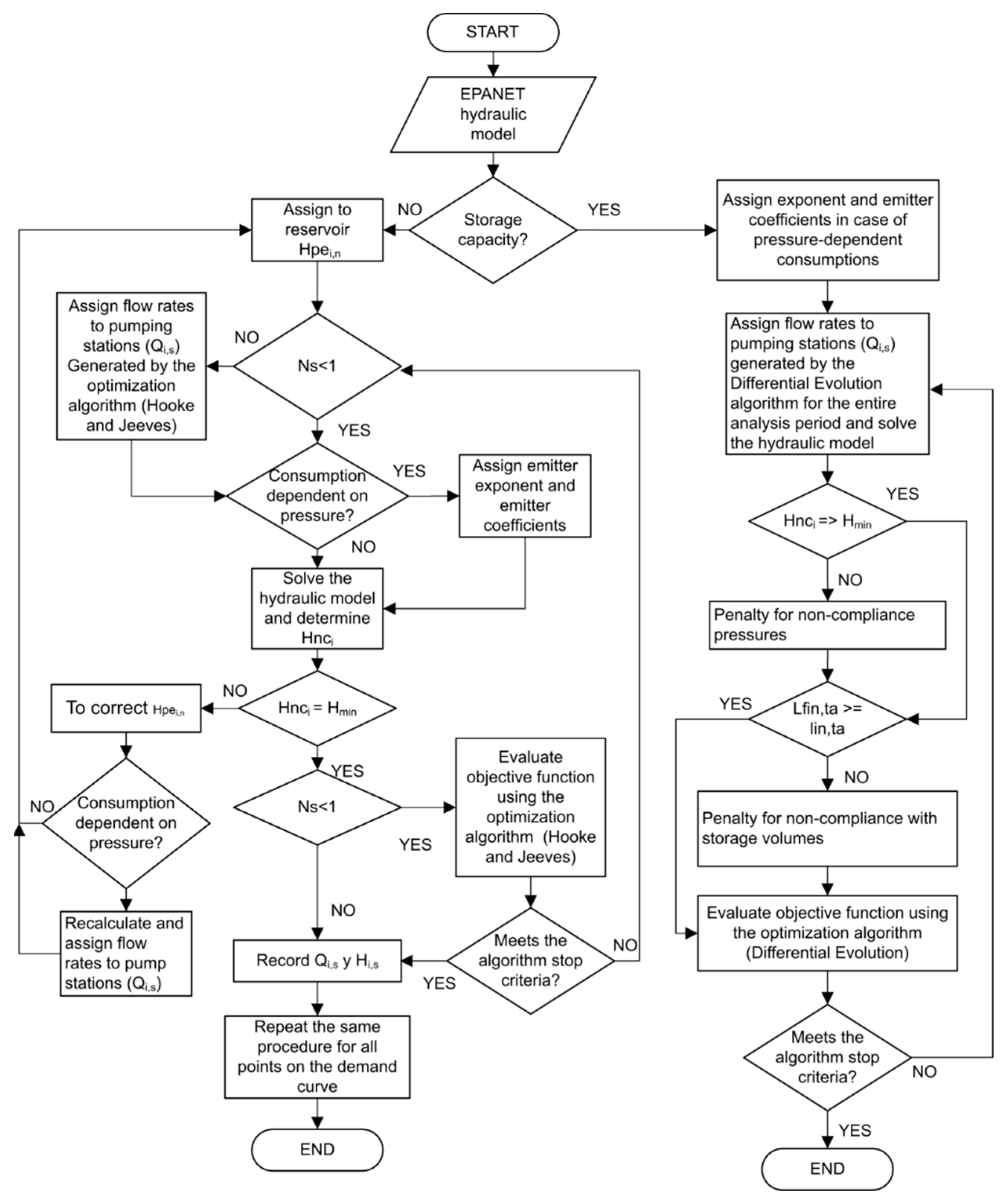
The differential evolution algorithm initially requires a population of Np solution vectors, and each solution vector will have dimensions for which the objective function will be evaluated. The algorithm follows three steps: mutation, crossing and selection. Mutation is the main sub-process of the methodology and consists of mutating the entire population through random selection and mathematical operations that occur between the solution vectors using an augmentation factor that controls the degree of the mutation. Crossing is nothing more than the combination of the elements that make up the mutated vectors with the elements of the vectors of the starting population to form new solution vectors; this process is also random. Selection refers to the choice of solution vectors that will make up a new population. If the new vectors obtained after the crossing produce better values of the objective function, they become part of the new generation. On the contrary, if the new solution vectors produce worse results, the vectors of the starting population will be preserved as members of the new generation. In this way, a new population is created that will be used to carry out a new search until the stopping criterion that has been defined is met. Figure 1 shows a scheme in which the process of the optimization of the setpoint curve is reflected as well as the implementation of the different algorithms.
3. Case Studies and Results
3.1. TF Network
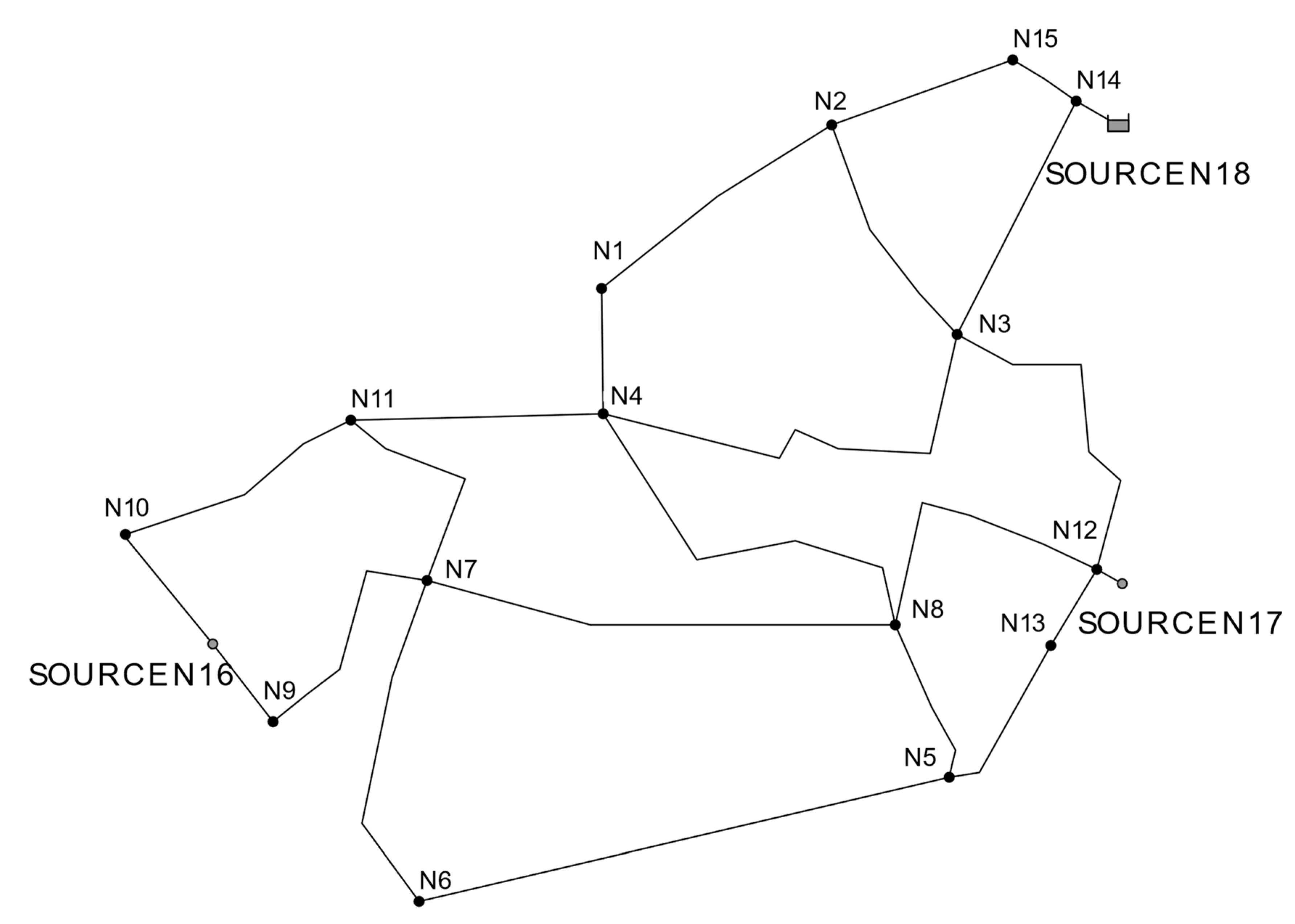
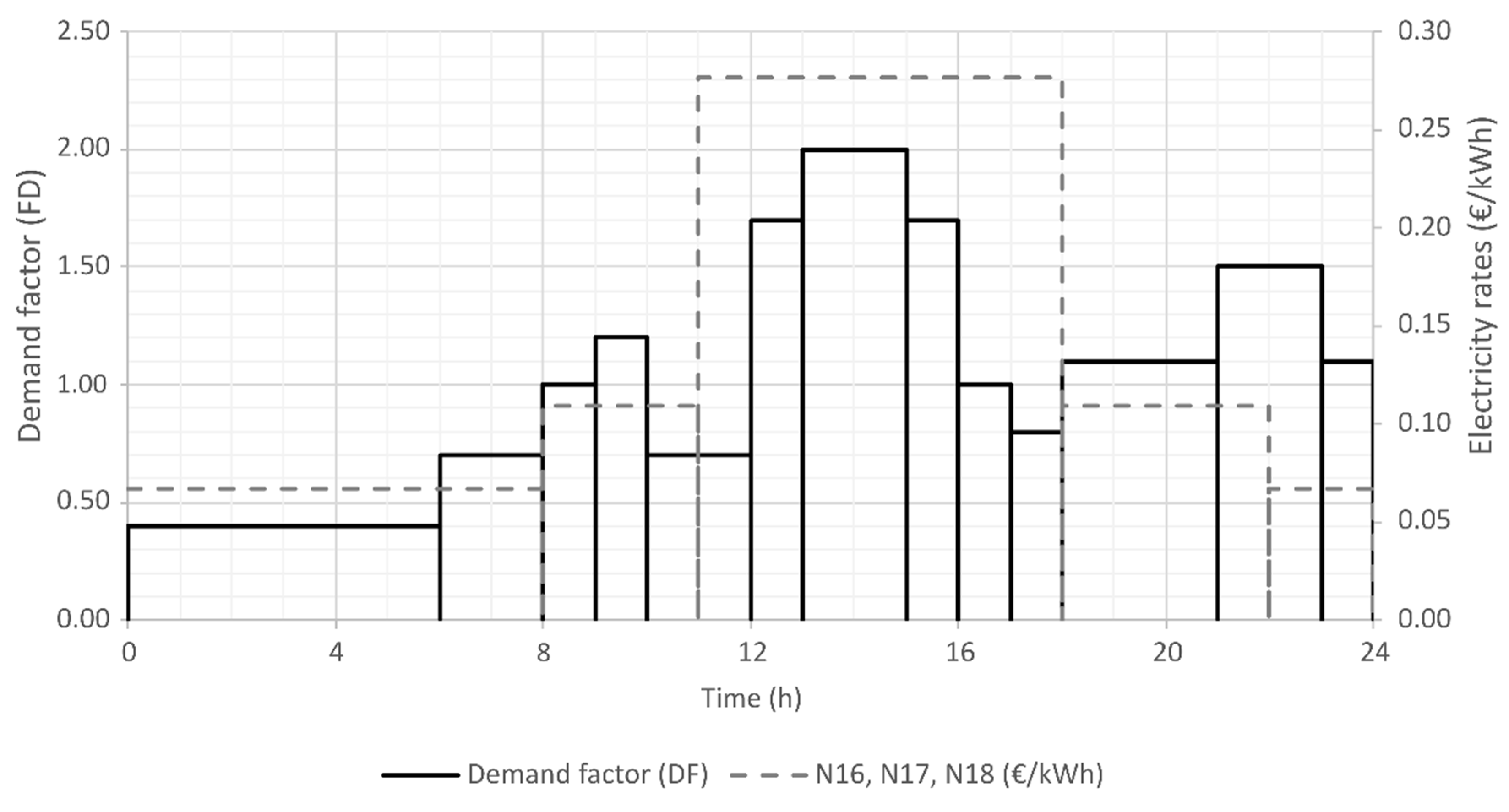
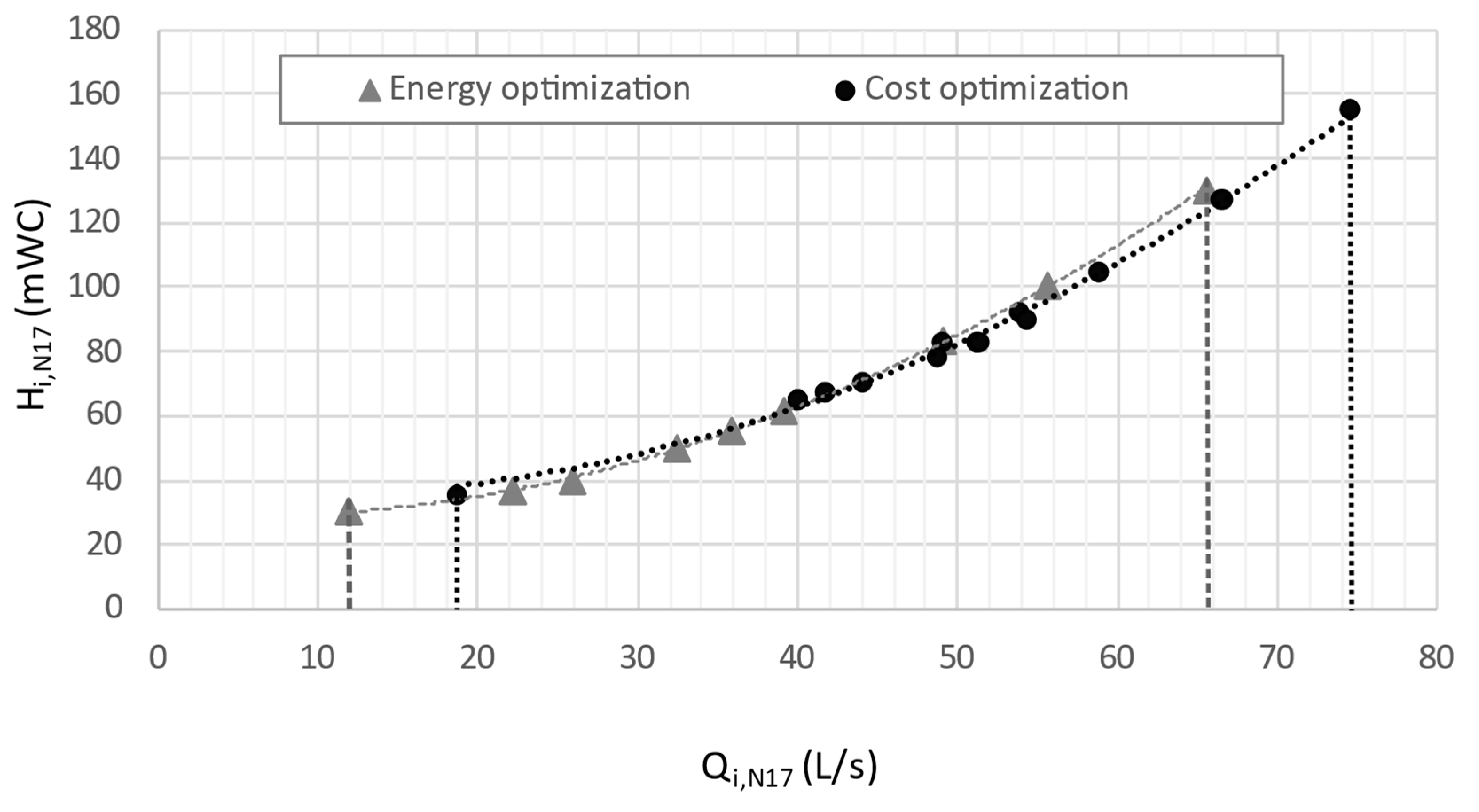
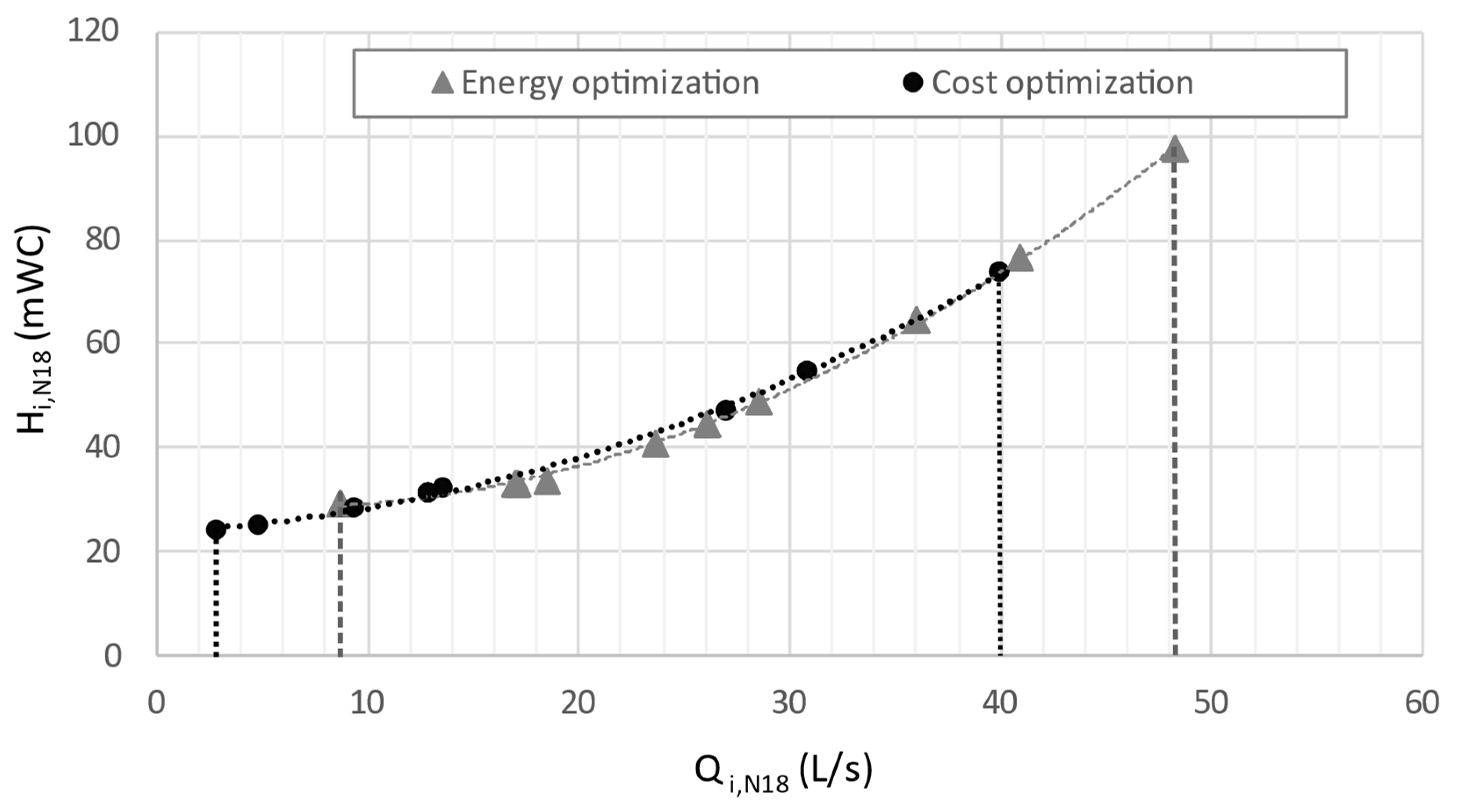
The first study case corresponds to the distribution network called TF in Figure 2 [7], which has three supply sources or pumping stations (N16, N17 and N18). Each pumping station is assigned an efficiency and a treatment rate that have been assumed constant regardless of time ( = 75%, = 0.25 €/m3; = 65%, = 0.20 €/m3; y = 60%, = 0.30 €/m3). The network has 17 nodes and a total of 24 pipes. The average daily flow is 100 L/s. The information on all the nodes as well as of the pipes is presented in Table 1 and Table 2. The roughness of all the pipes is 0.1 mm. The minimum pressure required in the network is = 20 mWC. The demand curve of the network, as well as the electricity rates, are presented in Table 3 and Figure 3.
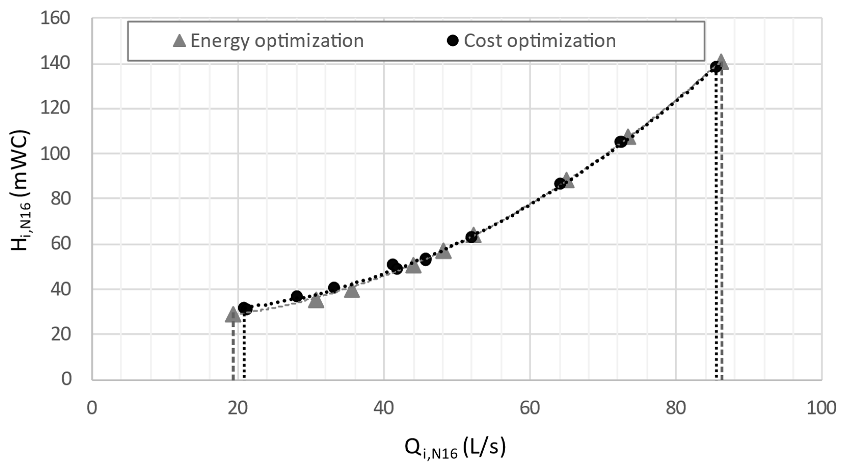
The network has been optimized first from a purely energy perspective, that is, without considering any cost, and then with adding the costs of both electricity rates and treatment rates, for which only the Hooke and Jeeves algorithm has been used. Figure 4, Figure 5 and Figure 6 show the setpoint curves obtained for each pumping station after having carried out the two types of optimization (energy and cost), which will undoubtedly be very useful when designing, selecting and regulating the pumps for each pumping station in the network.
It can be seen that within the same pumping station, the SC curves are very similar in terms of the pumping head, considering that the minimum pressure required is maintained at the critical node at all times. Therefore, in this case, it is evident that there is a single optimal setpoint curve in terms of minimum energy for each pumping station. The variations between curves presented when costs are included in the optimization are given for the range of flows that each station must supply, which is exposed in Figure 5 and Figure 6. In this sense, although the pressure heads are the same, the optimal flow distribution is different depending on whether they are considered costs or not.
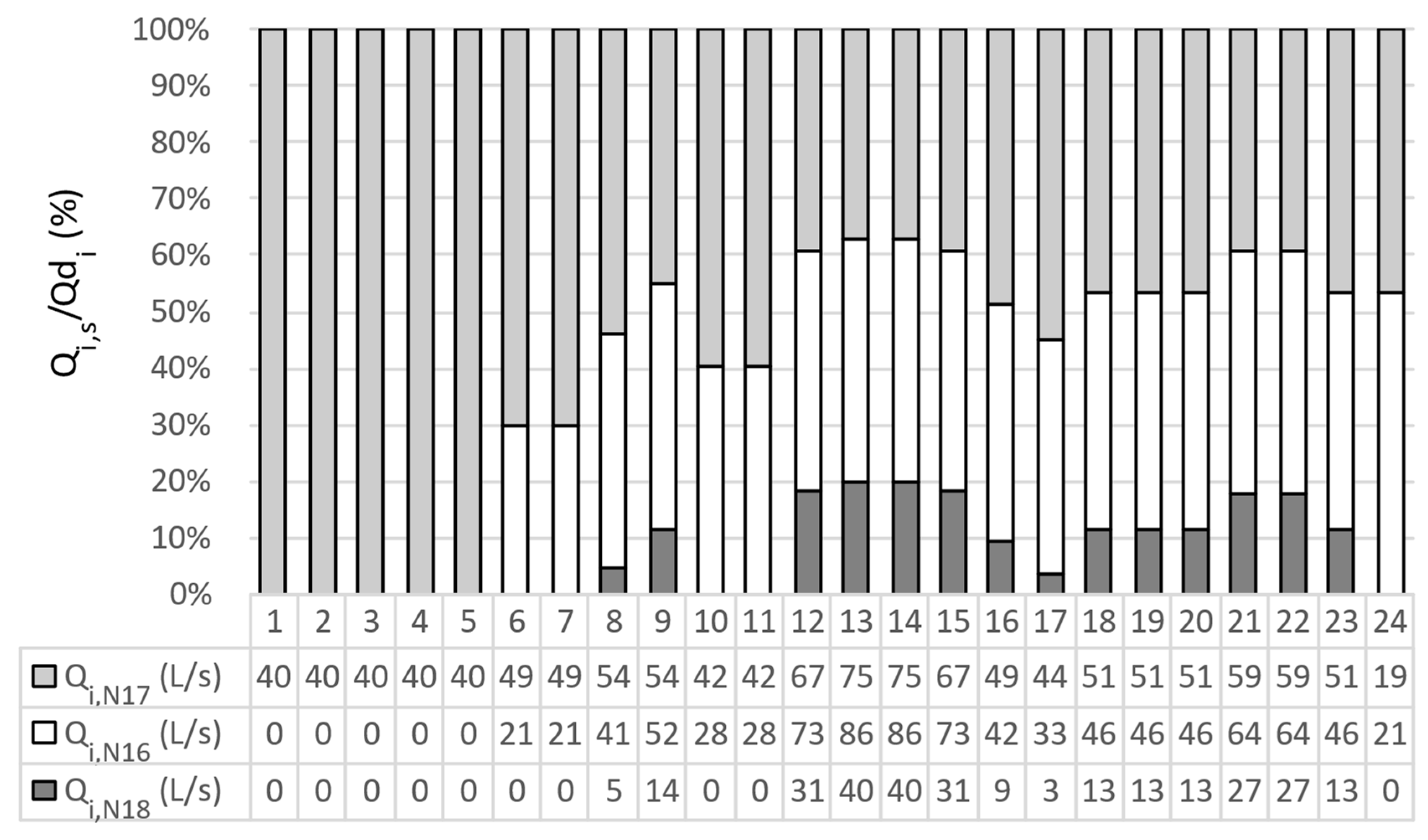
Figure 7 and Figure 8 show the optimal flow distribution between the pumping stations depending on the type of optimization.
In the case of energy optimization (Figure 7), the distribution remains almost constant. That is, for each point of the demand curve, the pumping stations supply practically the same flow percentage (N16 = 45%, N17 = 32%, and N18 = 23%). Furthermore, the pumping station N16 is the most important water source in the network in terms of energy, which is possibly due to its elevation of 4 m in relation to the other sources. On the contrary, as far as cost optimization is concerned, Figure 8 shows quite a different flow distribution where it is indicated which stations supply the network with more or less flow at different times of the day. In this case, the pumping station that involves the lowest costs is the N17 since it assumes the highest distribution flow, which is possibly due to the fact that it is the station that has the lowest treatment rate. On the other hand, station N18 works only 14 h a day, so there could be some additional study on the convenience of keeping said pumping station in operation.
The two types of optimization show the usefulness of the proposed methodology for obtaining the SC of each pumping station, as well as the optimal flow distribution between the different pumping stations when meeting two objectives, the reduction of energy consumption and cost minimization.
3.2. Richmond Network
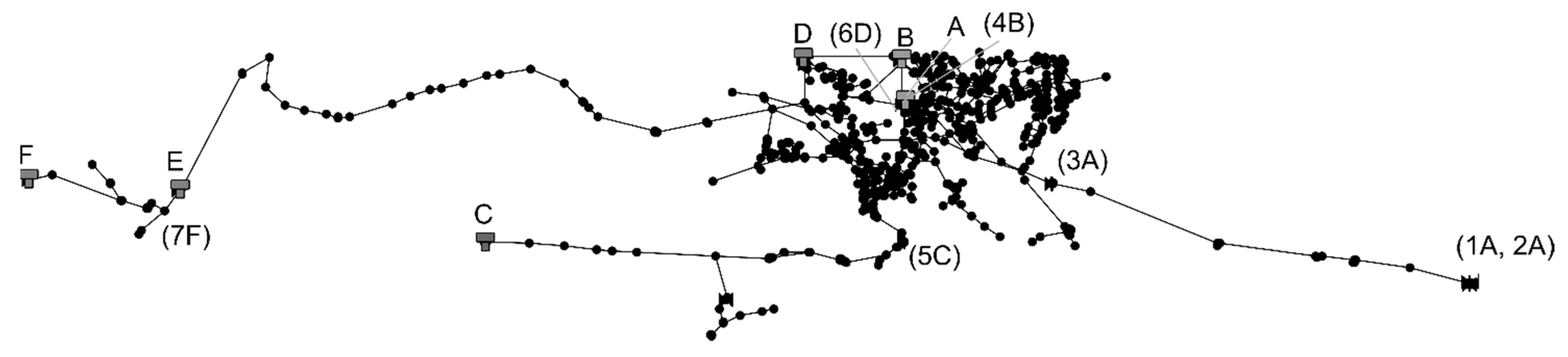
The Richmond water network distribution model is owned by Yorkshire Water in the United Kingdom and has been used for research on some methods of optimizing its operation [23,24]. This network (Figure 9) has a supply source with a variable suction level that has an associated pumping system (1A, 2A); it is also made up of five re-pumping stations (3A, 4B, 5C, 6D and 7F). There are six tanks (A, B, C, D, E and F). The nomenclature of the pumps indicates which tank they are associated with through the corresponding letter. Network details can be found on the Exeter University website [22].
The analysis of the network is based on the assumption that the operating pressures of the consumption nodes are met as long as the operating levels of the tanks are within the pre-established ranges (in other words, minimum and maximum levels). The objective is to find the optimal operating levels of the tanks, as well as the setpoint curves of the pumping stations that entail the minimum energy cost for a period of 24 h. Consequently, the objective function is the one given by Equation (7), where the network storage capacity is included. The differential evolution algorithm is applied in this case because the number of decision variables increases considerably. The data on the pumping stations are presented in Table 4, which contains the values of the minimum performance expected in each of the stations as well as a flow limitation, which is given by the capacity of the installed system.
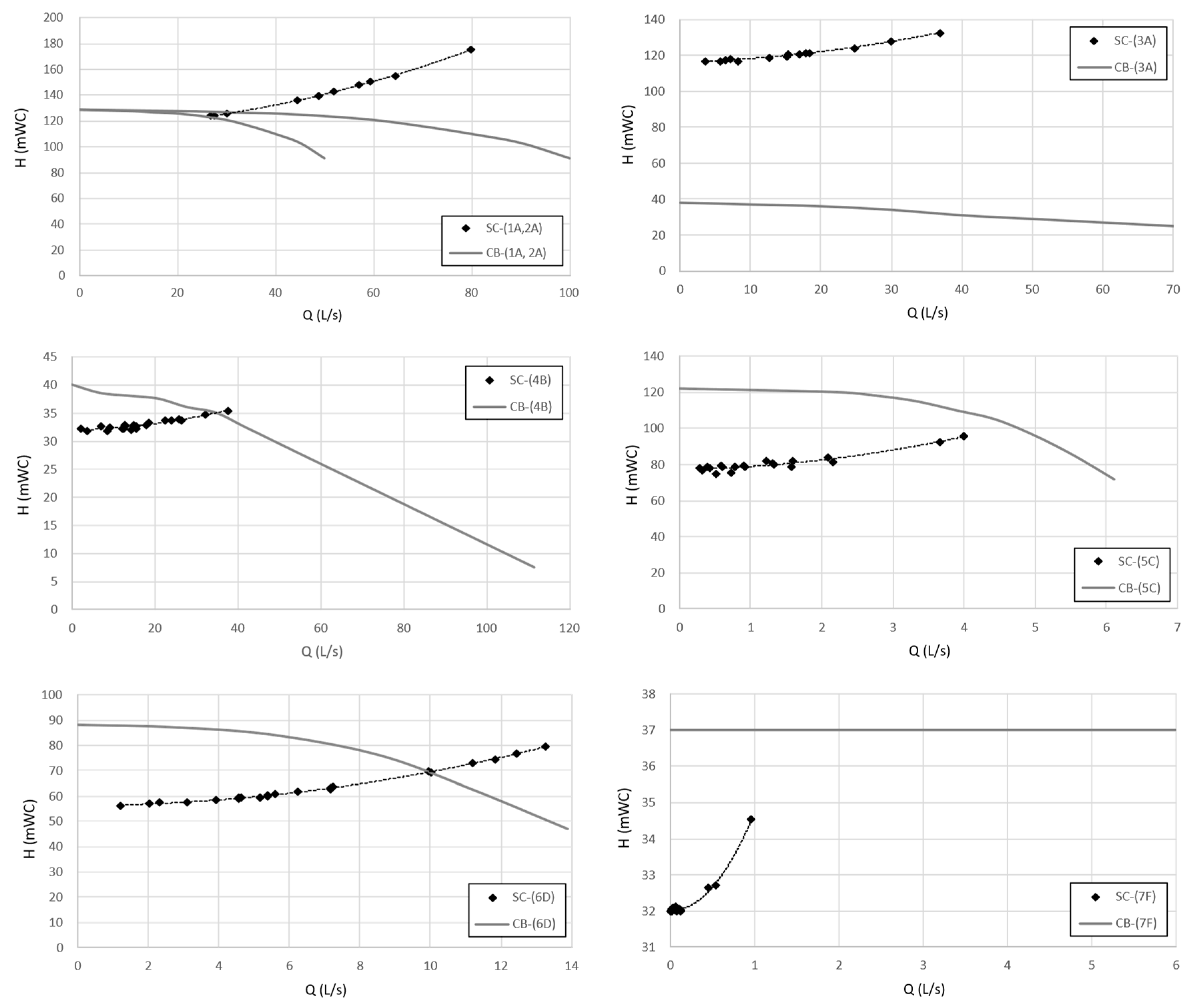
The information on the tanks is presented in Table 5, which includes the initial levels of the tanks at zero hours (0:00 h) that were obtained after carrying out the optimization process. At the Centre for Water Systems of Exeter University [22] a minimum operating cost of GBP 33,982, is stated, a value that is taken as a reference when analyzing the results obtained through the methodology proposed in the present study. The cost derived from the object method of this study is GBP 29,705.96 with a saving of 12.58%. Although the different optimization methodologies cannot be compared given the conceptual use of pumping stations, this value indicates the maximum savings that can be achieved once the driving curve of the installed pumping systems has been adjusted to the corresponding setpoint curve (Figure 10).
Figure 10 shows the setpoint curves (SC) obtained after optimization, as well as the curves of the installed pumps. It can be seen that in no case do the setpoint SCs exceed the range of flow rates that each pumping system is capable of providing. However, with regard to pumping heads, some of the pumping stations are undersized (1A–2A, 3A, 4B, 6D), so that in order to minimize the operating cost, it is necessary to install pumps that allow compliance with the pumping heads indicated by the setpoint curves. Additionally, the results reflect that the systems (1A–2A) and (3A) installed in series have similar pumping heads and therefore that station 3A does not fulfill the expected re-pumping functions, such that it may be feasible to eliminate said station or eliminate the bypass that makes pumping station 3A work in the same conditions as 1A–2A. In the case of the remaining pumping stations (5C and 7F), although the stations have sufficient capacity to satisfy the SC, they are oversized. It is important to note that since the current system is made up of fixed speed pumps, it is necessary to implement flow and pumping head regulation systems that allow for adjusting the driving curves of the pumps with the corresponding setpoint curves. In this way, the proposed methodology allows for knowing the maximum savings in operating costs that a pumping system is capable of achieving as long as it is possible to adjust to the corresponding setpoint curve.
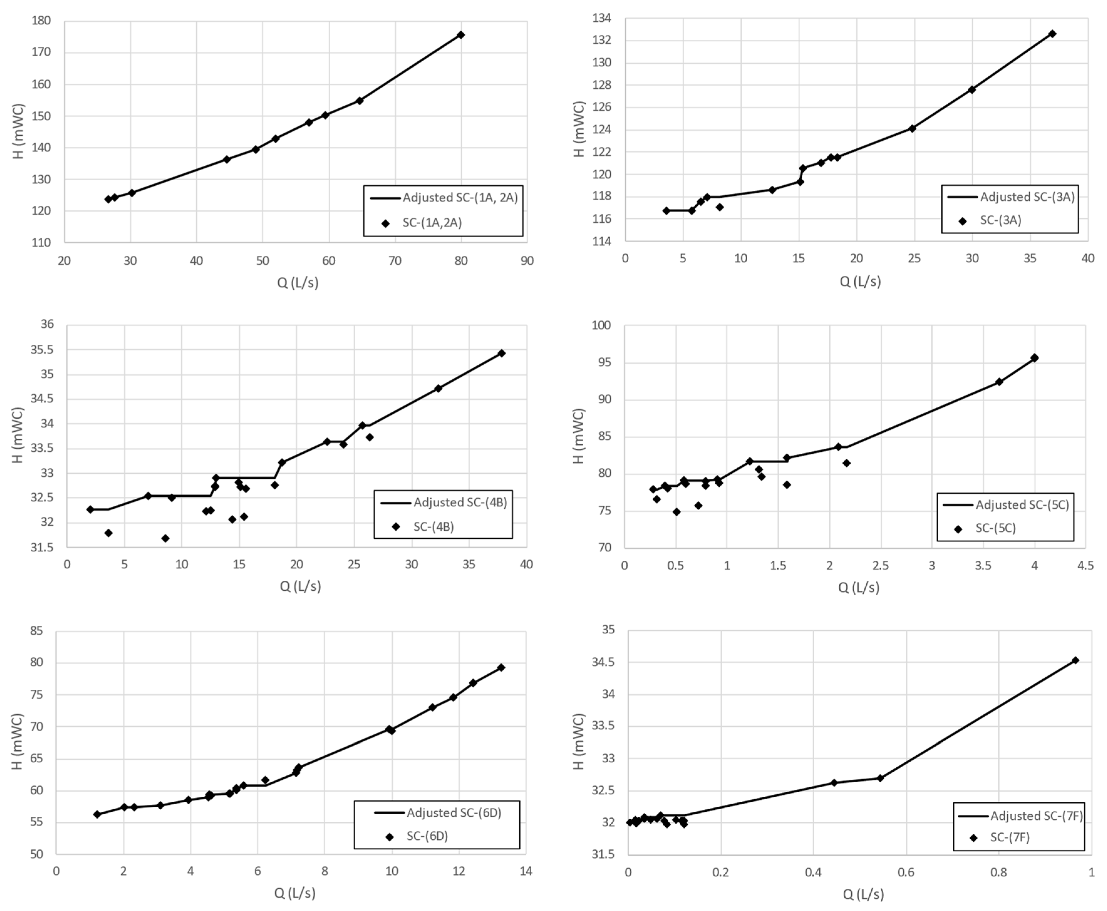
For energy and cost optimization in which storage capacity is not included, the shape of the SC is quite well defined. This does not happen in the case of networks with tanks, mainly because it is not possible to maintain the minimum pressure at the critical node during the entire analysis period, but the pressure at said node will be equal to or greater than the minimum for the cases in which a higher pressure is needed when filling the tanks of the network, so the curve presents oscillations subject to variations in the tank levels. When this happens, it is necessary to readjust the SC so that it is possible to establish regulation setpoints in the pumping systems in the simplest way possible, as shown in Figure 11. This readjustment will undoubtedly have an impact on the minimum operating cost; in this case, the new minimum will be GBP 29,740.68 so the saving is reduced to 12.48%, a value that is still of considerable magnitude.
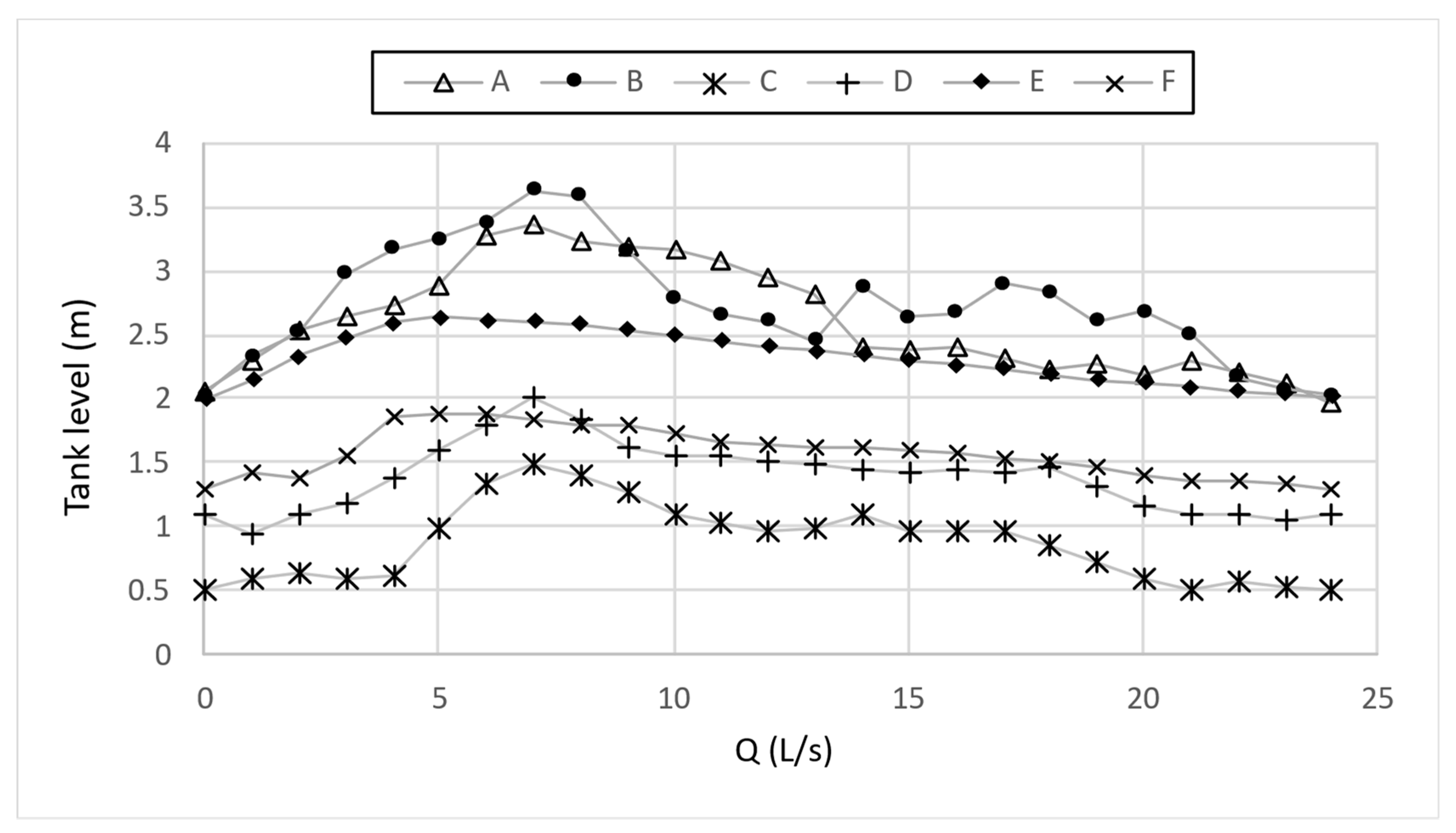
It has already been mentioned before that the concept of the setpoint curve implies maintaining the minimum possible pressure in the critical node of the network while maintaining the minimum energy costs through the optimal distribution of flows between the supply sources. The use of tanks (leaving aside the reliability of the network) implies an increase in pumping energy, as well as the pressure head at the nodes, which could lead to a considerable increase in operating costs depending on the management of electricity rates. Figure 12 shows the evolution of the levels of the tanks, some of which do not reach their maximum capacity; therefore, a part of the storage volume is underused (specifically tank C = 36.83% and F = 11.63%). In this way, it is not enough to manage storage solely from the perspective of managing electricity rates; it is also necessary to know the lifting height of each tank that is more favorable for cost savings. In this sense, SC has proven to be a useful tool for determining said elevation that can also be applied to the sizing of reserve tanks.
4. Discussion
Water and energy management are directly related and depend on water distribution networks operation (WDNs), involving scheduling pumps, regulating water levels of storage and providing satisfactory water quality to customers at required flow and pressure. Specifically, pump operating costs constitute the largest expenditure for water organizations worldwide. Traditionally, the pumps are selected based on a operation point, and subsequently, their operation is optimized once the equipment has been selected. In contrast, this work proposes an approximation of the operation mode of the pump in the planning phase, optimizing energy and cost in the WDN. This new approach can help to better select the pumping equipment.
The new methodology considers the following characteristics of the WDN: (a) with and without storage capacity, (b) with pressure-dependent and independent consumptions and (c) with multiple pumping stations whether they are water sources or pumping stations. All this is based on the concept of the setpoint curve (SC) and complies with the flow, pressure and storage volume constraints. This new approach is based on two fundamental pillars: (1) represent the pumping stations as flow injection nodes and (2) maintain the minimum possible pressure at the critical node of the network. The final objective is to determine the optimal Q-H (SC) curve for each pumping station that allows for meeting the demand of the network while keeping energy consumption to a minimum, as well as the minimum pumping cost.
Depending on whether the process for calculating the SC includes costs or not and whether there is storage capacity in the network, three objective functions have been formulated that will be used separately depending on the case of the study network. The first objective function consists of an optimization only of the energy type, where the values of Q and H for each pumping station that minimize the energy in the network become part of the corresponding SC. The second objective function considers the pumping costs by including the electricity rates with an hourly variation structure, as well as the the treatment costs, by adding a treatment rate associated with the source of water production from where pumping takes place. In this second function, there is no performance curve assigned to each pumping station because the SC curve is not that of a pump but rather a value of the minimum estimated performance expected in each of the pumping stations of the network.
The third objective function arises from the change in the procedure for calculating the SC when including the storage capacity of the network. This is mainly due to the fact that in the case of the first two functions, the calculation process implies keeping the pressure at the critical node equal to the minimum pressure required. However, when the use of tanks is included, there are times when the pressure in said node is higher since it is necessary to increase the pressure energy so that the tanks can be filled. Therefore, the pressure at the critical node is variable and unknown, which is why it is included as a penalty cost within the objective function as long as it is below the established value. Another added cost, also a penalty, is that of the volume of the reservoir tanks for the case in which the levels at the end of the simulation period are below the initial levels. In this way, a function with four costs is obtained: pumping cost, treatment cost, penalty cost for noncompliance in the pressure and penalty cost for noncompliance in the storage levels of the tanks.
The proposed methodology has been applied to two study networks, the TF network and the Richmond network, whose main difference lies in the presence of tanks. For the TF network, both energy and cost optimization have been carried out through the inclusion of electricity rates. As a result, the optimal setpoint curves for the three pumping stations have been obtained.
In relation to optimization algorithms, two have been used: Hooke and Jeeves and differential evolution. Both algorithms respond to a multidimensional, nonlinear problem without an analytical solution subject to constraints. Hooke and Jeeves has been applied only in the case of calculating the SC without storage capacity, that is, for the first two optimization functions, which is mainly due to the fact that the number of dimensions is low and is equivalent to the number of sources or network pumping stations. Although this algorithm has problems with local optimum, it is efficient enough when obtaining the optimal SC for each pumping station since the search space is mostly limited by the constraints of the SC calculation process. Additionally, since there is no storage capacity, the optimization is for static hydraulic models and can be executed separately for each demand of the network, which considerably speeds up the process.
On the other hand, the differential evolution algorithm has only been applied in the case of distribution networks with tanks, that is, the third of the objective functions. The use of another algorithm is because the number of dimensions of the problem increases considerably, which is due to the fact that including the tanks, the analysis of the hydraulic model is dynamic insomuch that the number of decision variables is given by the product between the number of pumping stations and the number of hours or number of scenarios that make up the analysis period. However, unlike Hooke and Jeeves, the differential evolution algorithm is designed to handle a large number of variables and does not present problems with local optimum.
5. Conclusions
A new mathematical model to minimize energy and cost optimization in a WDN based in the concept of the setpoint curve (SC) is proposed. This new approach is based on representing the pumping stations as flow injection nodes and maintaining the minimum possible pressure at the critical node of the network. Some network topologies were considered: (a) with and without storage capacity, (b) with pressure-dependent and independent consumptions and (c) with multiple pumping stations whether they are water sources or pumping stations.
Two case studies were presented, the TF network and the Richmond network. The main difference between the two case studies is the presence of tanks. This represents significant differences in the calculation of the SC and in the subsequent optimization process, since it greatly increases the number of decision variables. According to the results, it is possible to state the following:
- If the WDN have tanks, the critical node pressure is dependent on the tank level. Consequently, the setpoint curves present oscillations with respect to the required pumping heads because it is not possible to maintain a constant pressure at the critical node of the network. However, it is possible to know the maximum savings that can be obtained as long as it is possible to adjust the curve of each pumping system to the corresponding setpoint curve, hence the usefulness when determining if a system is over- or under-dimensioned.
- The use of the setpoint curve allows for evaluating whether raising the storage tanks represents a significant economic saving, although this aspect requires a deeper analysis.
- Given that the setpoint curve depends to a large extent on the pressure at the critical node, it is possible to combine the methodology with sectorization processes with the intention of better managing the pressure of the network and leading to greater savings in energy costs.
- The studied concept can also serve as a methodology for sizing tanks that correspond to pumping stations capable of adapting to optimal setpoint curves and that further minimize operating costs.
To summarize, the proposed methodology allows for obtaining the optimal flow distribution as well as the range of flows and the minimum pumping heads that lead to the minimum energy consumption and costs in the network. Consequently, the presented methodology is useful for the selection and implementation of pumping regulation systems.
Finally, by always maintaining the minimum pressure in the network, leaks are reduced; therefore, it may be convenient to analyze how significant the savings derived from there are.
Author Contributions
Conceptualization, C.F.L.-C., P.L.I.-R. and F.J.M.-S.; data curation, C.F.L.-C. and D.M.-M.; formal analysis, C.F.L.-C., P.L.I.-R., F.J.M.-S. and D.M.-M.; funding acquisition D.M.-M.; investigation, C.F.L.-C., P.L.I.-R., F.J.M.-S. and D.M.-M.; methodology C.F.L.-C., P.L.I.-R. F.J.M.-S. and D.M.-M.; project administration P.L.I.-R. and F.J.M.-S.; resources, C.F.L.-C., P.L.I.-R., F.J.M.-S. and D.M.-M.; software, C.F.L.-C., P.L.I.-R., F.J.M.-S. and D.M.-M.; supervision, P.L.I.-R., F.J.M.-S. and D.M.-M.; validation, C.F.L.-C., P.L.I.-R., F.J.M.-S. and D.M.-M.; visualization, C.F.L.-C., P.L.I.-R., F.J.M.-S. and D.M.-M.; writing—original draft, C.F.L.-C., P.L.I.-R., F.J.M.-S. and D.M.-M.; writing—review & editing, C.F.L.-C., P.L.I.-R., F.J.M.-S. and D.M.-M. All authors have read and agreed to the published version of the manuscript.
Funding
This research was funded by the Program Fondecyt Regular, grant number 1210410.
Data Availability Statement
Not applicable.
Acknowledgments
This work was supported by the Program Fondecyt Regular (Project 1210410) of the Agencia Nacional de Investigación y Desarrollo (ANID), Chile.
Conflicts of Interest
The authors declare no conflict of interest.
Nomenclature
| Symbols | |
| Q | Demand flow |
| H | Head pressure |
| Hpei,n | Pressure head of the reservoir |
| Hnci,n | Pressure head of the critical node |
| Hei | Pumping head of the station represented by the reservoir |
| Hi,s | Pumping head of each station (s) for the simulation period (i) |
| Qe,i | Flow supplied by the reservoir |
| Qi,s | Flow to be supplied by each pumping station (s) during the analysis period (i) |
| Qdi | Flow demanded during a simulation period (i) |
| Qmaxi,s | Maximum flow supplied by each pumping station (s) during the analysis period (i) |
| Qmini,s | Minimum flow supplied by each pumping station (s) during the analysis period (i) |
| Qmd | Average daily demand flow |
| Hmin | Minimum required pressure |
| lin,ta | Initial level of the tank |
| lfin,ta | Final level of the tank |
| Nta | Total numbers of tanks |
| η(i,s) | Performance of the station (s) during the period (i) |
| ti | Pumping time that corresponds to the duration of the simulation period (i) |
| Tfi,s | Electricity rate assigned to the station (s) for the period (i) |
| Abbreviations | |
| SC | Setpoint Curve |
| TT | Treatment rate |
| FD | Demand factor |
| WDN | Water Distribution Network |
References
- Dadar, S.; Đurin, B.; Alamatian, E.; Plantak, L. Impact of the pumping regime on electricity cost savings in urban water supply system. Water 2021, 13, 1141. [Google Scholar] [CrossRef]
- Goulter, I.C. Systems Analysis in Water-Distribution Network Design: From Theory to Practice. J. Water Resour. Plan. Manag. 1992, 118, 238–248. [Google Scholar] [CrossRef]
- Martin-Candilejo, A.; Santillán, D.; Iglesias, A.; Garrote, L. Optimization of the design of water distribution systems for variable pumping flow rates. Water 2020, 12, 359. [Google Scholar] [CrossRef] [Green Version]
- Casasso, A.; Tosco, T.; Bianco, C.; Bucci, A.; Sethi, R. How can we make pump and treat systems more energetically sustainable? Water 2019, 12, 67. [Google Scholar] [CrossRef] [Green Version]
- Filipe, J.; Bessa, R.J.; Reis, M.; Alves, R.; Póvoa, P. Data-driven predictive energy optimization in a wastewater pumping station. Appl. Energy 2019, 252, 113423. [Google Scholar] [CrossRef] [Green Version]
- Martínez-Solano, F.; Iglesias-Rey, P.; Mora-Meliá, D.; Fuertes-Miquel, V. Using the Set Point Concept to Allow Water Distribution System Skeletonization Preserving Water Quality Constraints. Procedia Eng. 2014, 89, 213–219. [Google Scholar] [CrossRef] [Green Version]
- León-Celi, C.; Iglesias-Rey, P.L.; Martinez-Solano, F.J.; Mora-Melia, D. A Methodology for the Optimization of Flow Rate Injection to Looped Water Distribution Networks through Multiple Pumping Stations. Water 2016, 8, 575. [Google Scholar] [CrossRef] [Green Version]
- Pasha, M.F.K.; Lansey, K. Optimal Pump Scheduling by Linear Programming. In Proceedings of the World Environmental and Water Resources Congress 2009—World Environmental and Water Resources Congress 2009: Great Rivers, Kansas, MO, USA, 17–21 May 2009; pp. 395–404. [Google Scholar] [CrossRef]
- McCormick, G.; Powell, R.S. Derivation of near-optimal pump schedules for water distribution by simulated annealing. J. Oper. Res. Soc. 2004, 55, 728–736. [Google Scholar] [CrossRef] [Green Version]
- Candelieri, A.; Perego, R.; Archetti, F. Bayesian optimization of pump operations in water distribution systems. J. Glob. Optim. 2018, 71, 213–235. [Google Scholar] [CrossRef] [Green Version]
- Wu, P.; Lai, Z.; Wu, D.; Wang, L. Optimization Research of Parallel Pump System for Improving Energy Efficiency. J. Water Resour. Plan. Manag. 2015, 141, 04014094. [Google Scholar] [CrossRef]
- Wu, Z.Y.; Zhu, Q. Scalable parallel computing framework for pump scheduling optimization. In Proceedings of the World Environmental and Water Resources Congress 2009—World Environmental and Water Resources Congress 2009: Great Rivers, Kansas, MO, USA, 17–21 May 2009; Volume 342, pp. 430–440. [Google Scholar] [CrossRef]
- Hashemi, S.S.; Tabesh, M.; Ataeekia, B. Ant-colony optimization of pumping schedule to minimize the energy cost using variable-speed pumps in water distribution networks. Urban Water J. 2014, 11, 335–347. [Google Scholar] [CrossRef]
- Wegley, C.; Eusuff, M.; Lansey, K. Determining pump operations using particle swarm optimization. In Proceedings of the Joint Conference on Water Resource Engineering and Water Resources Planning and Management 2000: Building Partnerships, Minneapolis, MN, USA, 30 July–2 August 2000; Volume 104. [Google Scholar] [CrossRef]
- López-Ibáñez, M. Operational Optimisation of Water Distribution Networks. Ph.D. thesis, Edinburgh Napier University, Edinburgh, Scotland, UK, 2009. [Google Scholar]
- Ormsbee, L.E.; Lansey, K.E. Optimal Control of Water Supply Pumping Systems. J. Water Resour. Plan. Manag. 1994, 120, 237–252. [Google Scholar] [CrossRef] [Green Version]
- Mala-Jetmarova, H.; Sultanova, N.; Savic, D. Lost in Optimisation of water distribution systems? A literature review of system design. Water 2018, 10, 307. [Google Scholar] [CrossRef] [Green Version]
- León-Celi, C.F.; Iglesias-Rey, P.L.; Martínez-Solano, F.J.; Savic, D. Operation of Multiple Pumped-Water Sources with No Storage. J. Water Resour. Plan. Manag. 2018, 144, 04018050. [Google Scholar] [CrossRef]
- Hooke, R.; Jeeves, T.A. Direct search solution of numerical and statical problems. J. ACM 1961, 8, 212–229. [Google Scholar] [CrossRef]
- Storn, R.; Price, K. Differential evolution—A Simple and Efficient Heuristic for Global Optimization over Continuous Spaces. J. Glob. Optim. 1997, 11, 341–359. [Google Scholar] [CrossRef]
- Rossman, L.; Woo, H.; Tryby, M.; Shang, F.; Janke, R.; Haxton, T. EPANET 2.2 User Manual; EPA/600/R-20/133; U.S. Environmental Protection Agency: Washington, DC, USA, 2020. [Google Scholar]
- Centre for Water Systems, “University of Exeter”. 2022. Available online: http://emps.exeter.ac.uk/engineering/research/cws/resources/benchmarks/#a7 (accessed on 1 July 2022).
- van Zyl, J.E.; Savic, D.A.; Walters, G.A. Operational Optimization of Water Distribution Systems Using a Hybrid Genetic Algorithm. J. Water Resour. Plan. Manag. 2004, 130, 160–170. [Google Scholar] [CrossRef]
- Giacomello, C.; Kapelan, Z.; Nicolini, M. Fast Hybrid Optimization Method for Effective Pump Scheduling. J. Water Resour. Plan. Manag. 2013, 139, 175–183. [Google Scholar] [CrossRef]
Figure 1.
General flow chart of the cost minimization process.

Figure 2.
The TF distribution network.

Figure 3.
Demand pattern and electricity rates.

Figure 4.
Setpoint curve for pumping station N16.

Figure 5.
Setpoint curve for pumping station N17.

Figure 6.
Setpoint curve for pumping station N18.

Figure 7.
Flow distribution in the case of energy optimization.

Figure 8.
Flow distribution in the case of cost optimization.

Figure 9.
Richmond distribution network.

Figure 10.
Setpoint curves (SC) and characteristic curves of the pumps (CB) for the pumping stations of the Richmond network.
Figure 10.
Setpoint curves (SC) and characteristic curves of the pumps (CB) for the pumping stations of the Richmond network.

Figure 11.
Readjusted setpoint curves for pumping stations on the Richmond network.

Figure 12.
Evolution of tank levels in the Richmond network.


Table 1.
Nodes of the TF network.
| ID | Elev (m) | Demand (L/s) | ID | Elev (m) | Demand (L/s) |
|---|---|---|---|---|---|
| N1 | 8 | 5 | N10 | 7 | 5 |
| N2 | 8 | 4 | N11 | 7 | 10 |
| N3 | 5 | 3 | N12 | 5 | 5 |
| N4 | 8 | 4 | N13 | 4 | 2 |
| N5 | 4 | 3 | N14 | 3 | 10 |
| N6 | 2 | 8 | N15 | 3 | 15 |
| N7 | 5 | 7 | N16 | 4 | 0 |
| N8 | 6 | 10 | N17 | 0 | 0 |
| N9 | 2 | 9 | N18 | 0 | 0 |
Table 2.
Pipes of the TF network.
| Node 1 | Node 2 | Lenght (m) | Diam. (mm) | Node 1 | Node 2 | Lenght (m) | Diam. (mm) |
|---|---|---|---|---|---|---|---|
| N1 | N2 | 200 | 150 | N11 | N7 | 300 | 80 |
| N2 | N3 | 150 | 100 | N11 | N4 | 250 | 150 |
| N3 | N4 | 150 | 100 | N8 | N12 | 250 | 80 |
| N4 | N1 | 200 | 200 | N5 | N13 | 100 | 60 |
| N5 | N6 | 200 | 60 | N3 | N12 | 98 | 60 |
| N7 | N8 | 400 | 80 | N3 | N14 | 300 | 80 |
| N6 | N7 | 300 | 60 | N14 | N15 | 500 | 80 |
| N8 | N5 | 300 | 80 | N2 | N15 | 400 | 100 |
| N8 | N4 | 250 | 150 | N16 | N10 | 125 | 100 |
| N7 | N9 | 300 | 100 | N12 | N13 | 52 | 60 |
| N10 | N11 | 300 | 100 | N17 | N12 | 1 | 2000 |
| N9 | N16 | 125 | 100 | N14 | N18 | 1 | 1000 |
Table 3.
Demand curve and electricity rates.
| Time (h) | 1–5 | 6–7 | 8 | 9 | 10 | 11 | 12 | 13–14 | 15 | 16 | 17 | 18–20 | 21 | 22 | 23 | 24 |
|---|---|---|---|---|---|---|---|---|---|---|---|---|---|---|---|---|
| Demand factor (DF) | 0.4 | 0.7 | 1.0 | 1.2 | 0.7 | 0.7 | 1.7 | 2.0 | 1.7 | 1.0 | 0.8 | 1.1 | 1.5 | 1.5 | 1.1 | 0.4 |
| N16, N17, N18 (Є/kWh) | 0.0672 | 0.1094 | 0.2768 | 0.1094 | 0.0672 | |||||||||||
Table 4.
Maximum flow and expected performance of the pumping stations of the Richmond network.
| ID Source | Maximum Flow (L/s) | Performance (%) |
|---|---|---|
| (1A, 2A) | 100.00 | 75 |
| (3A) | 70.00 | 77 |
| (4B) | 111.50 | 72 |
| (5C) | 6.11 | 71 |
| (6D) | 13.89 | 58 |
| (7F) | 6.00 | 54 |
Table 5.
Richmond network tank information.
| ID Tanks | Diameter (mm) | Initial Level (m) | Min Level (m) | Max Level (m) |
|---|---|---|---|---|
| A | 23.5 | 2.050 | 1.02 | 3.37 |
| B | 15.4 | 2.030 | 2.03 | 3.65 |
| C | 6.6 | 0.500 | 0.50 | 2.00 |
| D | 11.8 | 1.100 | 1.10 | 2.11 |
| E | 8.0 | 1.992 | 0.20 | 2.69 |
| F | 3.6 | 1.293 | 0.19 | 2.19 |
Publisher’s Note: MDPI stays neutral with regard to jurisdictional claims in published maps and institutional affiliations. |
© 2022 by the authors. Licensee MDPI, Basel, Switzerland. This article is an open access article distributed under the terms and conditions of the Creative Commons Attribution (CC BY) license (https://creativecommons.org/licenses/by/4.0/).
Share and Cite
MDPI and ACS Style
León-Celi, C.F.; Iglesias-Rey, P.L.; Martínez-Solano, F.J.; Mora-Melia, D. The Setpoint Curve as a Tool for the Energy and Cost Optimization of Pumping Systems in Water Networks. Water 2022, 14, 2426. https://doi.org/10.3390/w14152426
AMA Style
León-Celi CF, Iglesias-Rey PL, Martínez-Solano FJ, Mora-Melia D. The Setpoint Curve as a Tool for the Energy and Cost Optimization of Pumping Systems in Water Networks. Water. 2022; 14(15):2426. https://doi.org/10.3390/w14152426
Chicago/Turabian StyleLeón-Celi, Christian F., Pedro L. Iglesias-Rey, Francisco Javier Martínez-Solano, and Daniel Mora-Melia. 2022. "The Setpoint Curve as a Tool for the Energy and Cost Optimization of Pumping Systems in Water Networks" Water 14, no. 15: 2426. https://doi.org/10.3390/w14152426
Note that from the first issue of 2016, this journal uses article numbers instead of page numbers. See further details here.