
Prediction and Interpretation of Water Quality Recovery after a Disturbance in a Water Treatment System Using Artificial Intelligence


1
Department of Civil and Environmental Engineering, Hanbat National University, 125, Dongseo-daero, Yuseong-gu, Daejeon 34158, Korea
2
GNC Environmental Solution, 201, 24, Umuk-gil 52beon-gil, Chuncheon-si 24368, Korea
3
Waterworks Research Institute, Waterworks Headquarters Incheon Metropolitan City, 332, Bupyeong-daero, Bupyeong-gu, Incheon 22101, Korea
4
Department of Environmental Research, Korea Institute of Civil Engineering and Building Technology, 283, Goyang-daero, Ilsanseo-gu, Goyang-si 10223, Korea
*
Author to whom correspondence should be addressed.
Water 2022, 14(15), 2423; https://doi.org/10.3390/w14152423
Submission received: 7 July 2022
/
Revised: 2 August 2022
/
Accepted: 3 August 2022
/
Published: 5 August 2022
(This article belongs to the Section Water Quality and Contamination)
Abstract
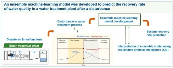
:In this study, an ensemble machine learning model was developed to predict the recovery rate of water quality in a water treatment plant after a disturbance. XGBoost, one of the most popular ensemble machine learning models, was used as the main framework of the model. Water quality and operational data observed in a pilot plant were used to train and test the model. Disturbance was determined when the observed turbidity was higher than the given turbidity criteria. Therefore, the recovery rate of water quality at a time t was defined during the falling limb of the turbidity recovery period. It was considered as a relative ratio of the differences between the peak and observed turbidities at time t to the difference between the peak turbidity and turbidity criteria. The root mean square error–observation standard deviation ratio of the XGBoost model improved from 0.730 to 0.373 by pretreatment, removing the observation for the rising limb of the disturbance from the training data. Moreover, Shapley value analysis, a novel explainable artificial intelligence method, was used to provide a reasonable interpretation of the model’s performance.
1. Introduction
Safety management in water resources and drinking water systems is an important issue that requires global efforts to improve public health. Various contaminants in streams and reservoirs used for drinking water supply threaten public health, and water treatment plants are crucial public facilities for providing safe water to the public. Thus, the optimization of water treatment plant operations is essential for the stable supply of safe drinking water.
The quality of drinking water produced in a water treatment plant is affected by various factors, including the quality of raw water, the composition of water treatment facilities, and the operational conditions of the treatment processes. Natural disasters, such as typhoons, heavy rains, and earthquakes, are also important factors that should be considered for the proper management of water treatment plants [1,2,3]. The effect of a disaster on a water supply system is often observed based on various conditions, including damage to pipelines, destruction of pumping systems, and malfunctioning of electrical operational systems [4,5]. The damage to water treatment plants caused by natural disasters cause consequent malfunctions in the water treatment system. This results in abnormal water quality in the water treatment process, such as increased turbidity, contamination, and leakage of drinking water. One common accident in water treatment plant operations is the suspension of coagulants (e.g., poly aluminum chloride) owing to the malfunction of the agent supply system. This malfunction results in an increase in the turbidity of the subsequent processes, which represents the status of disturbance in the water treatment process. Turbidity is the most widely used index that quantitatively represents the status of water quality in a drinking water treatment plant. An increase in turbidity represents an increase in the degree of contamination, including organic materials, nutrients, and heavy metals [6,7].
Considering the proper management of water supply systems, the prediction of water quality caused by various malfunctions, including disasters, is essential. Recent studies have provided a methodological approach using statistical methods or advanced machine learning to predict or quantify the damage to social infrastructure caused by various disasters [4,8,9]. Inoue et al. [10] used deep learning and support vector machines for anomaly detection in water treatment plants [11]. Recently, Chen and Guestrin [12] developed an ensemble risk assessment model to determine the risk grade of rainstorm disasters in target areas using random forest (RF) and deep neural networks. The application of machine learning for the management of water treatment systems is still being studied. Furthermore, water quality in drinking water supply systems is difficult to predict because various physical, chemical, and biological factors affect the quality of drinking water produced in water treatment plants [6,11,13].
Practically, post-disaster management is crucial for the proper management of water treatment systems. Recovery or post-disaster management is an emerging issue in the management of public infrastructure [14,15]. Moreover, studies on the application of advanced machine learning models to predict water quality in water resources and water treatment systems have increased [16,17,18,19]. However, studies on the quantification and prediction of recovery stages in water treatment plants after disasters and related disturbances are still at an early stage.
Artificial neural networks (ANNs) were some of the first machine learning algorithms to be developed, and various advanced algorithms (e.g., ensemble machine and deep learning algorithms) have been continuously developed to overcome the limitations of previous models. For example, deep learning has been developed to overcome the limitations of conventional ANNs, such as vanishing gradients and overfitting [20,21,22]. Tree-based ensemble machine learning models, such as RFs and gradient boosting decision trees (GBDTs), are some of the most popular and widely used machine learning models. Ensemble machine learning models have been increasingly applied in water quality management studies recently [23,24]. The ensemble model is composed of multiple independent tree-based models known as weak learners, and model performance can be improved by determining the final model prediction obtained by combining the results of each weak learner [25,26,27].
This study provides a methodological approach to quantify the recovery rates of water quality after the occurrence of malfunctions in water treatment plants. Considering the first part of the study, an ensemble machine learning model was developed to predict recovery rate by the following steps: (i) the recovery rate was defined as the change in turbidity after disturbance in the water treatment process; and (ii) a machine learning model was developed from pilot-scale field operational data, with XGBoost (XGB), the most popular GBDT algorithm, being used as the main structure of the model framework. Regarding the second part of the study, explainable artificial intelligence (XAI) was used to provide an understandable interpretation of the model’s performance. A machine learning model is often referred to as a black box model. A limitation on the practical application of a machine learning model for managing water treatment plants is that the results from the machine learning model are hardly interpretable. Recently, Dunnington et al. [28] compared the performance of a physically based model with that of three machine learning models in predicting organic carbon removal in a water treatment system. Their study emphasized the importance of model result interpretability in the practical application of machine learning models. The XAI is a novel method that provides an interpretation of the performance of a machine learning model based on characteristics and relationships. Therefore, it overcomes an important limitation of black box-based machine learning models and improves the practicability of advanced machine learning models [29,30,31]. In this study, a novel XAI method, the Shapley value (SHAP), was used to analyze the model’s performance and provide an understandable interpretation of the model’s predictions [32].
2. Materials and Methods
2.1. Pilot Plant Operation
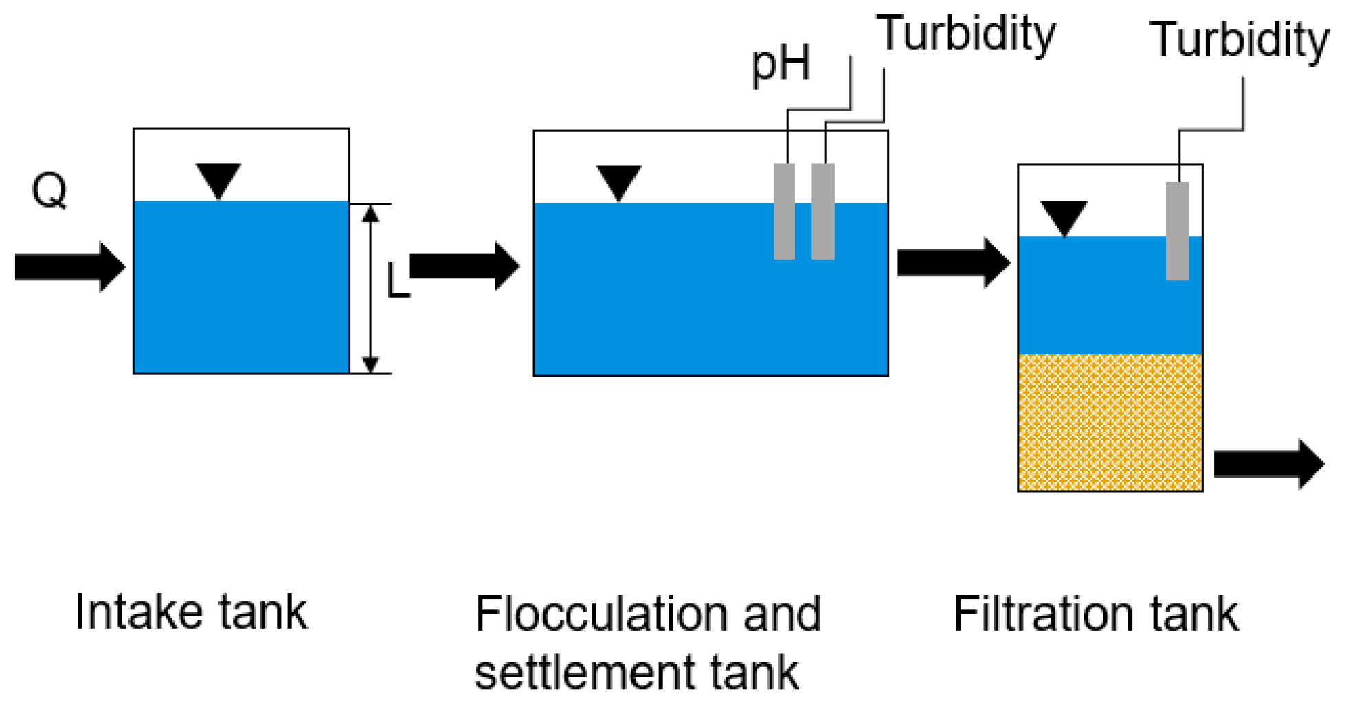
Operational data for water treatment processes were measured in a pilot-scale water treatment plant (pilot plant) (Figure 1) located at the Bupyung Water Treatment Plant Office in Incheon City, South Korea. The processes applied at the pilot plant involved an intake tank, a flash-mix tank, a flocculation and settlement tank, and a filtration tank. The hourly water quality observational data from the pilot plant were used for the model development in this study, as shown in Table 1. Hourly turbidity and pH were measured using electronic sensors, the water level was measured using an ultrasonic level sensor, and the flow rate was measured using an electromagnetic sensor.
2.2. Model Development
2.2.1. Definition of the Recovery Rate
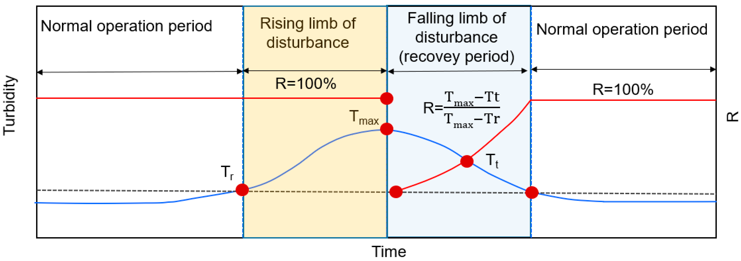
The turbidity of water after filtration is one of the most representative indices of water quality status. First, the criteria for abnormal turbidity (Tr) were determined, and the disturbance period was defined as the period when the observed turbidity was higher than Tr, as shown in Figure 2. Thus, the disturbance period started after the observed turbidity became higher than the criterion Tr. Moreover, the turbidity increased continuously until it reached the maximum turbidity during the disturbance (Tmax). Thereafter, the turbidity decreased until it became lower than Tr. The recovery rate (R) of turbidity at time t during the falling limb of the disturbance was determined from the relative ratio of the differences between Tmax and Tt to the differences between Tmax and Tr (1). R was calculated from the instance immediately after the turbidity reached Tmax to the instance the turbidity decreased below Tr. Defining the recovery rate in this study, R is considered as 100% during the rising limb of the turbidity after the disturbance.
R (%): recovery rate of turbidity during the falling limb disturbance at time t;
(NTU): maximum turbidity during a disturbance event;
: criteria for abnormal water quality;
: turbidity observed at time t.
2.2.2. Operation Scenario
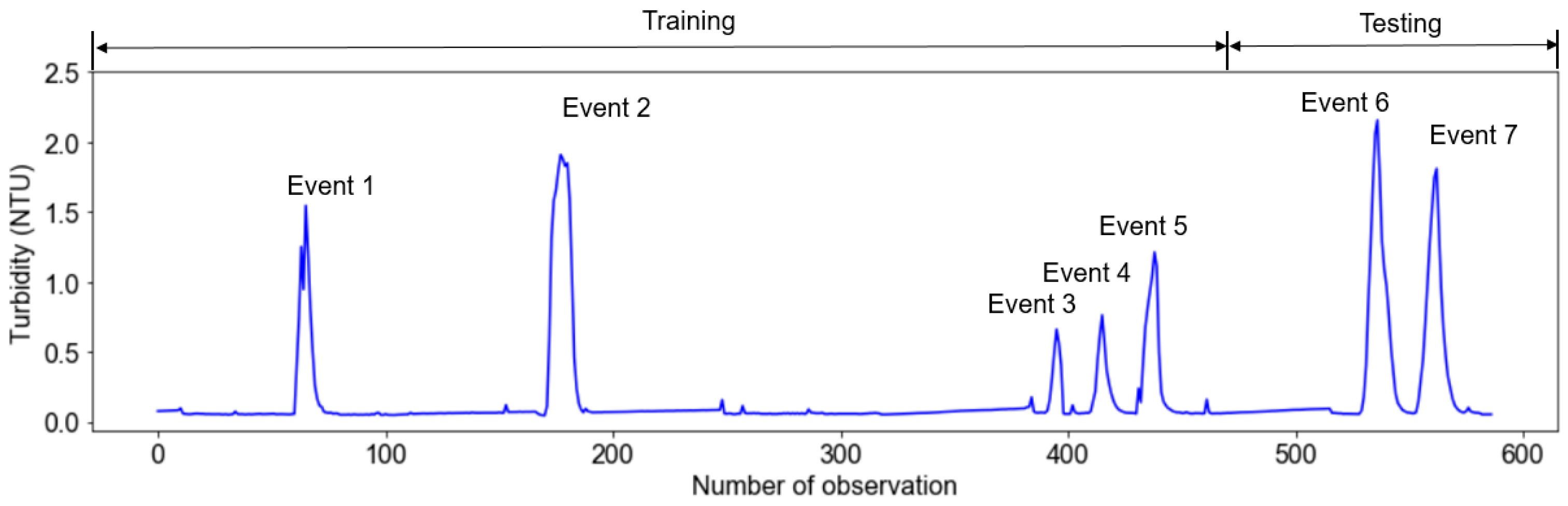
Disturbance with respect to water quality caused by an accident was simulated in the pilot plant. The fine particles in the water were aggregated into larger-sized particles by adding a coagulant so that the particles were removed in the succeeding filtration process. The suspension of the coagulant thus caused increased turbidity in the water treatment process, including in the filtration tank. In this study, there were seven events of disturbance imitated by the suspension of coagulant (poly aluminum chloride 12%) inputted during the entire operation period (Table 2). The observed data during the observation period (Table 2), including the simulated disturbance period, were used for the training and testing of a machine learning model to predict R during the falling limb disturbance in the water treatment process.
2.2.3. Data Split for the Training and Testing of the Model
The observed data for the four observation periods (Periods 1–4 in Table 2) were used for model development. A total of 469 observations from 21 September 2020 to 26 February 2021 and 118 observations from 27 February 2021 to 5 March 2021 were used for the training and testing of the machine learning model, respectively (Figure 3). The ratio of the data used for training and testing of the machine learning model was 80:20.
2.2.4. Input Variables
Five observed input variables (Table 1) were used as independent variables for model development, and the recovery rate, R, calculated using (1), was used as the dependent variable predicted by the model. The turbidity of the effluent in the filtration tank, TB_R3, is approximately 0.05 NTU in normal conditions, and peak TB_R3 ranged from 0.50 NTU to 2.16 NTU in the imitated abnormal condition. The criterion for the abnormal condition T was determined as 0.1 NTU. Furthermore, R was calculated from the turbidity value in the filtration tank (TB_R3) during the falling limb of TB_R3.
2.2.5. Pretreatment of the Input Variable
The proposed model predicted the recovery rate R during the falling limb of the disturbance period. During the rising limb of the disturbance, recovery was not calculated because the peak point of the disturbance cannot be estimated until it reaches the peak value. Thus, R was considered to be 100% (normal status) in both the normal operation period and the rising limb of the disturbance period (Figure 2). The model considered this status by training it using a dataset that excluded the rising part of the data. The rising part was determined using a logical (2). The data that fulfilled the logical condition in (2) at time t were excluded from the training dataset. This pretreatment was not applied to the test data. The model performances with pretreatment using (2) (Model 1) and without pretreatment (Model 2) were compared by training the model for each case.
If Tout > Tr and Tt+1 > Tt
: observed turbidity at time t;
: observed turbidity at time t+1.
2.2.6. Post-Treatment of Machine Learning Results
R was only defined during the falling limb of the disturbance period, and R during the rising limb was determined as R = 100%. The logical (3) was used for the model prediction result during the rising limb of disturbance as a post-treatment to consider this status in the machine learning developed in this study. Regarding (3), R at time t+1 was considered as 100%; therefore, R at the peak of the rising limb in the model prediction was determined as 100%. Considering the definition of the recovery rate, the predicted R was also determined as 100% when it was larger than 100%.
If Tout > Tr and Tt+1 > Tt, then Rt+1 = 100%
2.3. Machine Learning Model Selection
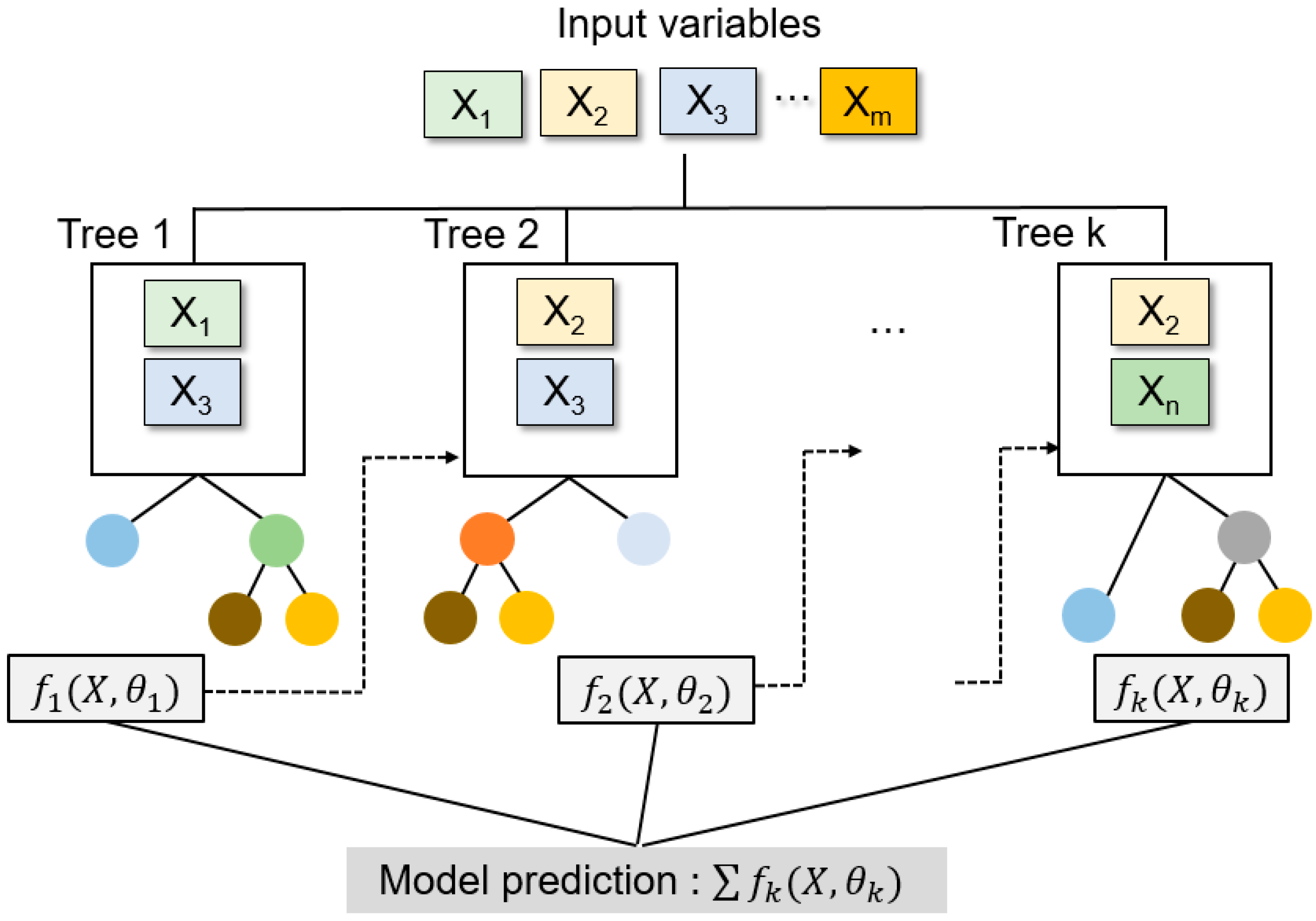
The recovery rate, R, is determined based on the change in turbidity, which is affected by the condition of the water quality in previous processes in water treatment plants. In this study, the GBDT, a tree-based ensemble learning algorithm, was used to predict the recovery rate after disturbance in a water treatment plant. The GBDT and the RF are popular ensemble learning models [33,34,35]. The RF is composed of multiple individual decision tree models, where the average of the individual decision tree models is determined as the final result of the model prediction. In contrast, the GBDT is composed of a sequence of decision tree models known as weak learners (Figure 4). The results of the previous decision tree model affect the results of the subsequent decision tree model by assigning a higher weight to data with higher residual errors in the previous decision tree model. Through this process, model performance is improved in the subsequent step [25,26].
The GBDT is optimized by minimizing the objective function, which is composed of two parts: the loss function (l) and the regularization function (), where X is an input variable and is an independent and identically distributed random vector ((4), (5) and Figure 4) [36]. The loss function (l) represents the total sum of the differences between the observation () and the model prediction () in each decision tree model for all the input data samples (n). The regularization function reduces complexity and prevents overfitting of the machine learning model (5). In (4), corresponds to an individual k-decision tree with weight , TL is the number of leaves on the tree, represents the complexity of each leaf, and is a parameter that scales the penalty [12,36].
In this study, XGB, one of the most popular GBDT models, was used to develop an ensemble machine learning model to predict recovery rates in water treatment processes after disturbance. The model was developed using the Python XGB library [12,36,37,38], where the hyperparameters of the model were optimized by a grid search method using the scikit-learn grid search library [37].
2.4. Model Evaluation
Three evaluation indices were used to evaluate the prediction performance of the XGB model: the Nash–Sutcliffe efficiency (NSE), root mean square error (RMSE), and RMSE–observation standard deviation ratio (RSR) (6)–(8). The value of NSE ranges from −∞ to 1, where NSE approaches 1 when the model prediction shows a better fit with the observations. The RMSE values ranged from 0 to ∞. The RMSE is calculated from the root-squared mean of the squared differences between the observation and prediction. A smaller RMSE represents a better model prediction performance. The value of the RSR ranges from 0 to 1, where the RSR approaches 0 when the model prediction shows a better fit with the observation. The model prediction is considered satisfactory when RSR < 0.70 [39,40].
: model prediction;
: observation;
: mean of the observed values.
2.5. XAI for Model Interpretation
A machine learning model is often known as a black box model because of limitations on the understandable interpretations of model performance results. The XAI is a novel method for providing an understandable interpretation of how a model prediction is determined from the input variables used in the model’s development. Moreover, SHAP analysis is one of the most representative XAI algorithms that provides an interpretation of model performance by comparing model prediction results with different combinations of input variables [32]. The SHAP value was calculated for each input variable from the weighted mean of the marginal contribution of the input variable (9) [32]. Through this analysis, SHAP provides quantified values for the contribution of the target input variables with respect to model performance. In this study, SHAP analysis was used to provide an understandable interpretation of the contribution of the input variables to the model’s performance.
: SHAP of the ith input variable;
: set of all input variables;
: all subsets of input variables without the ith input variable;
: values of the input variables in S without the ith input variable;
: the data set that includes the ith input variable;
: prediction based on input .
3. Results and Discussion
3.1. Water Quality of the Pilot Plant
The characteristics of all input variables used for the model development are summarized in Table 3. The five variables observed in the pilot plant were used as independent variables, and the recovery rate, R, calculated using (2), was used as the dependent variable for the XGB model development.
3.2. Model Prediction of Recovery Rate
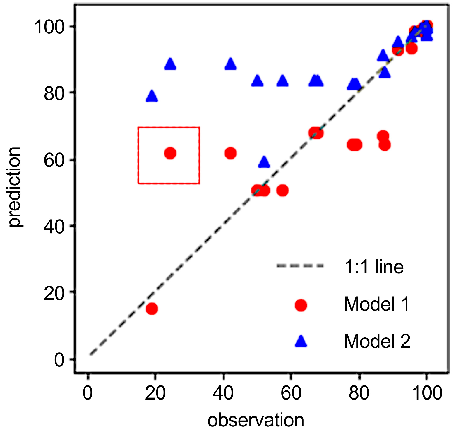
The performances of the two XGB models (Model 1 with pretreatment and Model 2 without pretreatment) were compared, and the two models were optimized with three hyperparameters (n estimator, max depth, and learning rate) using a grid search method. The optimal hyperparameters for each model are summarized in Table 4. The XGB model quantitatively predicted water quality recovery during the falling limb of the disturbance until the water quality recovered to a defined normal status. The observation and the prediction results of the two XGB models using the testing data are compared in Figure 5. The evaluation results show that the model’s performance is improved by the pretreatment of the input variables used for training the XGB model, where the prediction of Model 1 shows a better fit with a one-to-one line. The evaluation results of the two XGB models using these three indices are compared in Table 5. The values of NSE, RMSE, and RSR improved from 0.467 to 0.860, 10.310 to 5.280, and 0.730 to 0.374, respectively, when the rising limb of the turbidity in the filtration tank was excluded from the pretreatment process of the training data. Pretreatment was not applied to the test data. This result indicates that the XGB model is appropriately trained using the pretreatment process.
The model predictions of R in the two models were compared for two disturbance events (Events 6 and 7). The improvement of the XGB model using the pretreatment process is shown in Figure 6. Model 1 predicted the start and end periods of the disturbance for both events. The scale of recovery was also well predicted for Event 6, whereas the model underestimated the observations for Event 7.
3.3. Explainable Artificial Intelligence for Model Interpretation
3.3.1. SHAP
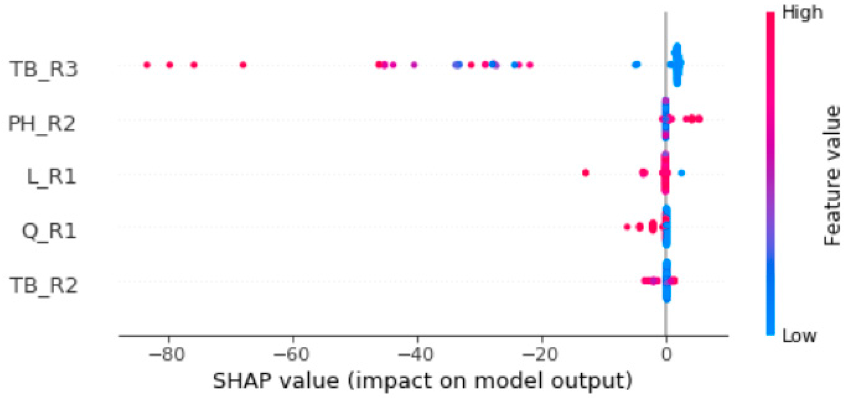
The prediction of a machine learning model is determined by the internal computation of the input variables. Thus, the result is affected by the complicated relationships between the input variables. SHAP analysis provided an understandable explanation of how the model simulation results were determined. The SHAP values represent the relative importance of the input variables in the XGB model. The colored dots in Figure 7 represent the distribution of SHAP for each observation. Considering Figure 7, the variables in the y-axis are sorted by the SHAP values for each variable in descending order. The color hue in Figure 7 represents the actual value of the observation. The red and blue colors indicate high and low observation values, respectively. The SHAP analysis suggests that the TB_R3 (the turbidity at the filtration process) is a factor that has the largest effect on the model simulation result. A larger negative SHAP value is observed when the observed TB_R3 is larger, as represented in red. Moreover, the SHAP value becomes close to zero and is slightly higher than zero when the observation becomes smaller, as represented in blue. This distribution of SHAP values indicates that the model prediction of R becomes larger when the observed turbidity in the filtration tank, TB_R3, becomes smaller. This corresponds to the actual relationship between TB_R3 and R, which indicates that the recovery rate increases to 100% as turbidity reduces until less than 0.1 NTU. The SHAP values for PH_R2 show that PH_R2 does not significantly affect R, whereas R tends to increase slightly when PH_R2 increases.
3.3.2. Exploratory Data Analysis with SHAP
The SHAP analysis also provides an explanation for the individual observations. Recent studies have used SHAP analysis to improve the interpretability of machine learning model results [31,41]. The SHAP force plot shows how model prediction is affected by individual observations. Figure 8a shows a SHAP force plot of an observation at 23:00 on 4 March 2021. Regarding this datum, the observed R was 24.29%, whereas the model prediction of R was 61.89%. This is an example of the considerable over-prediction of R, as indicated by the red dotted box in Figure 5.
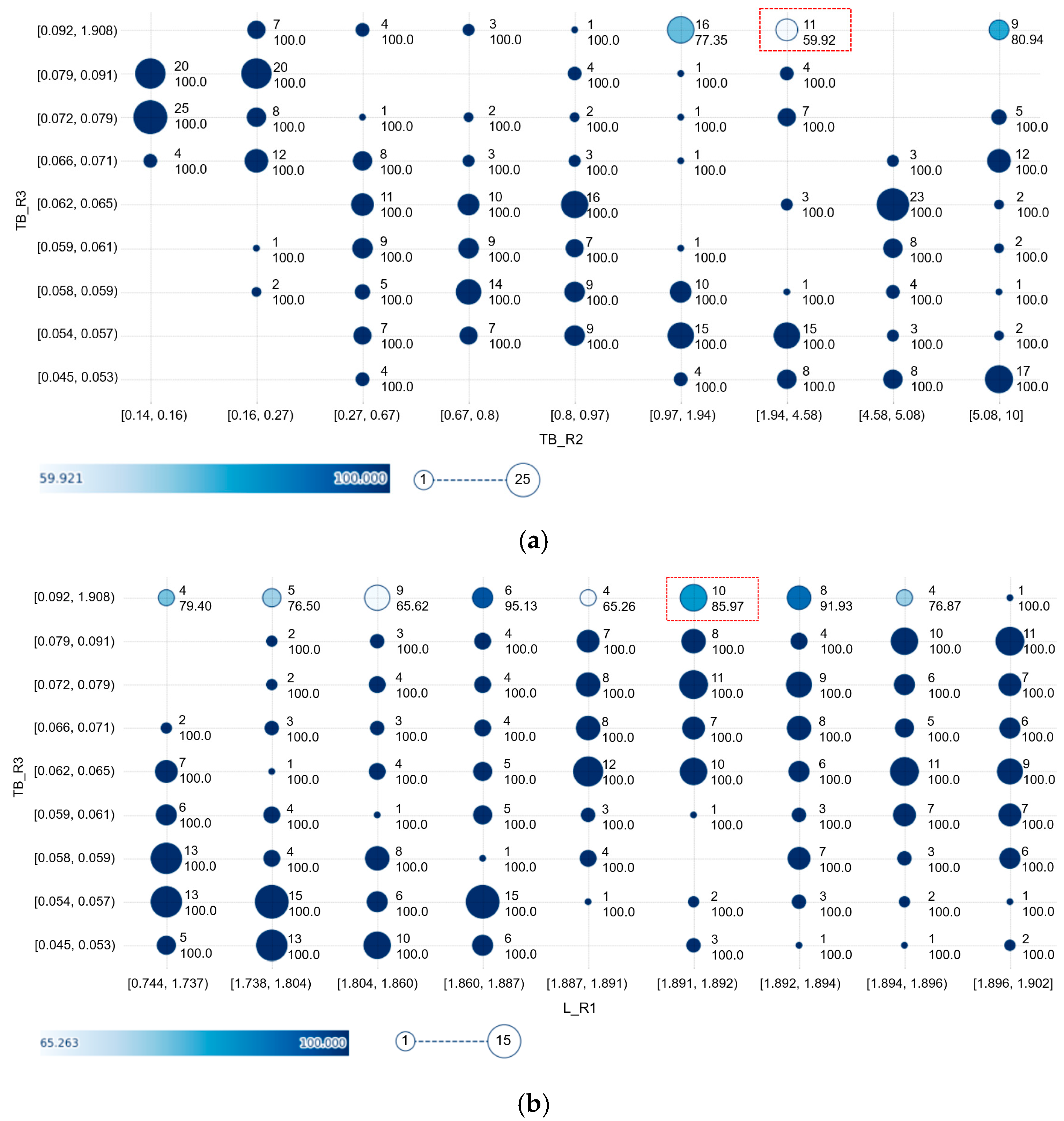
The SHAP force plot in Figure 8a shows that the model’s predicted R was 61.89%, when the observed TB_R3 was 1.394 NTU, and this observation of TB_R3 had the greatest effect in reducing the value of the predicted R. The effect of the other input variables on the model prediction was larger in the order of L_R1 and TB_R2. Although the observed input variables reduced the predicted R, the prediction was larger than the observed R. A possible interpretation for this over-prediction can be provided using SHAP analysis and exploratory data analysis (EDA). EDA is a method that analyzes data from various perspectives. The SHAP analysis showed that the model performance was affected by the input variables in the order TB_R3 > L_R1 > TB_R2. The relationship between the distribution of these input variables and R was explored using a target plot. Figure 9 is a target plot often used for EDA, where pdpbox, an open-source library, was used for plotting. Figure 9a shows the distribution of the observed R in the training data within a given range of the two input variables TB_R3 and TB_R2. For example, for the data in the TB_R2 range between 1.94 NTU and 4.58 NTU and in the TB_R3 range between 0.092 NTU and 1.908 NTU, the number of observed Rs within this range is 11, and the average of these 11 observed Rs is 59.92%, as marked in the red dotted box in Figure 9a. Thus, it can be inferred that the model is trained to predict a relatively higher R when the input variable is within this range. As a result of this training process, the model predicted an R of 61.89%. The observed R of 24.3% at 23:00 on 4 March 2021 is quite an exceptional case based on the distribution of other input variables and causes noticeable over-prediction by the XGB model. Another target plot for the input variables L_R1 and TB_R3 provides a similar interpretation. The observed L_R1 and TB_R3 were 1.891 m and 1.394 NTU at 23:00 on 4 March 2021, respectively. This observation falls in the range of L_R1 between 1.891 and 1.892 m and of TB_R3 between 0.092 to 1.908 NTU, as shown by the red dotted box in Figure 9b. There are ten observations with an average R of 85.97%. Since the model was trained from this relationship, the model over-predicted this case with an exceptionally low value for the observed R.
Considering the observation of the subsequent time step, at 00:00 on 5 March 2021, the observed and model predicted Rs were 49.93% and 50.44%, respectively. The observed TB_R3 and TB_R2 values still belong to the range marked by the red dotted box in Figure 9a. The force plot of data observed at 00:00 on 5 March 2021 in Figure 8b shows that the observed values of TB_R3 = 0.9556 NTU and TB_R2 = 3.054 NTU had the highest effect on model performance. It was estimated that the model exhibited good performance at this observation because the observation at 00:00 on 5 March 2021 was within the range of the distribution for the previous observation used for the training.
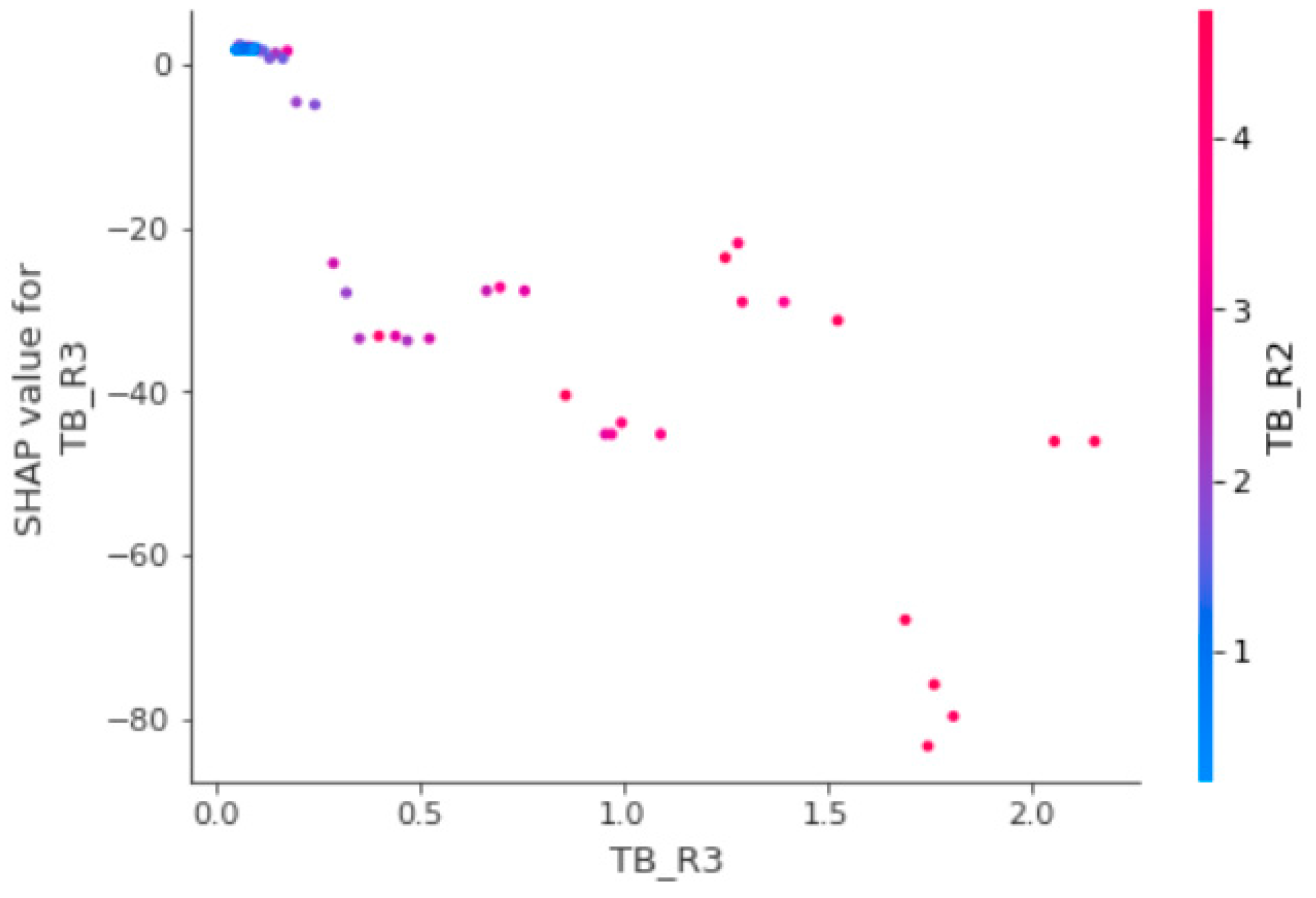
The influence of an input variable on the model’s performance is also explained using the SHAP dependence analysis (Figure 10). Regarding the SHAP dependency plot, the x-axis and the first y-axis represent the observed value of an input variable and the corresponding SHAP value of the input variable, respectively. The second y-axis represents the observed value of the interaction variable. Figure 10 shows that the SHAP value of TB_R3 decreased as TB_R3 increased. This relationship demonstrates that an increase in the observed TB_R3 value had a negative effect on the model prediction value, where the corresponding observed value of TB_R2 also increased.
4. Conclusions
In this study, the recovery rate of water quality in a water treatment plant after disturbance to the water treatment process was defined and an XGB model was developed to predict the recovery rate. Based on the definition of the recovery rate, a pretreatment process for the input data was used to improve the model’s performance. Considering the pretreatment process, the rising limb of turbidity was selectively removed from the training data used for the model’s development. Nevertheless, no pretreatment was applied to the data used to test the model’s performance. A considerable improvement in the model’s performance was observed with pretreatment of the input variables compared to the model’s performance without pretreatment. NSE, RMSE, and RSR improved from 0.467 to 0.860, 10.310 to 5.280, and 0.730 to 0.374, respectively, in the model with pretreatment.
Moreover, a novel XAI method was used to interpret the model’s performance. The analysis of model performance using the SHAP values for and the target plots of the training input variables provided a reasonable interpretation of the model’s prediction results.
The results obtained in this study demonstrate the applicability of a machine learning model for recovery prediction in water treatment processes after malfunctions. The importance of pretreatment of the data used in the model’s development, considering the characteristics of the input variables, has also been emphasized. The methodological approach presented in this study provides a useful approach for more stable and efficient management of water treatment systems.
Author Contributions
Conceptualization, J.P. (Jungsu Park), Y.Y. and J.P. (Jaehyeoung Park); methodology, J.P. (Jungsu Park), Y.Y. and J.P. (Jaehyeoung Park); software, J.P. (Jungsu Park); investigation, J.P. (Jungsu Park), J.A., J.K., Y.Y. and J.P. (Jaehyeoung Park); data curation, J.P. (Jungsu Park), J.A. and J.K.; writing—original draft preparation, J.P. (Jungsu Park); writing—review and editing, J.P. (Jungsu Park), Y.Y. and J.P. (Jaehyeoung Park); supervision, J.P. (Jaehyeoung Park); project administration, J.P. (Jaehyeoung Park); funding acquisition, J.P. (Jaehyeoung Park). All authors have read and agreed to the published version of the manuscript.
Funding
(1). This work was supported by Korea Environment Industry & Technology Institute(KEITI) through Environmental R&D Project on the Disaster Prevention of Environmental Facilities Program(or Project), funded by Korea Ministry of Environment(MOE)(2022002870001)(60%); (2). This work was supported by Korea Environment Industry & Technology Institute(KEITI) through Environmental R&D Project on the Disaster Prevention of Environmental Facilities Project, funded by Korea Ministry of Environment(MOE)(2019002870001) (30%); (3). This work was supported by the National Research Foundation of Korea (NRF) grant funded by the Korea government (MSIT) (No. 2020R1G1A1008377) (10%).
Conflicts of Interest
The authors declare no conflict of interest.
References
- Davis, C.A. Water system service categories, post-earthquake interaction, and restoration strategies. Earthq. Spectra 2014, 30, 1487–1509. [Google Scholar] [CrossRef]
- Matthews, J.C. Disaster resilience of critical water infrastructure systems. J. Struct. Eng. 2016, 142, C6015001. [Google Scholar] [CrossRef]
- WHO. Emergencies and Disasters in Drinking Water Supply and Sewage Systems: Guidelines for Effective Response; Pan American Health Organization: Washington, DC, USA, 2002; pp. 5–12. [Google Scholar]
- Park, J.; Park, J.-H.; Choi, J.-S.; Joo, J.C.; Park, K.; Yoon, H.C.; Park, C.Y.; Lee, W.H.; Heo, T.-Y. Ensemble model development for the prediction of a disaster index in water treatment systems. Water 2020, 12, 3195. [Google Scholar] [CrossRef]
- Shamsuzzoha, M.; Kormoker, T.; Ghosh, R.C. Implementation of water safety plan considering climatic disaster risk reduction in Bangladesh: A study on Patuakhali Pourashava water supply system. Procedia Eng. 2018, 212, 583–590. [Google Scholar] [CrossRef]
- Gaya, M.S.; Zango, M.U.; Yusuf, L.A.; Mustapha, M.; Muhammad, B.; Sani, A.; Tijjani, A.; Wahab, N.A.; Khairi, M.T.M. Estimation of turbidity in water treatment plant using Hammerstein-Wiener and neural network technique. Indones. J. Electr. Eng. Comput. Sci. 2017, 5, 666–672. [Google Scholar] [CrossRef]
- Iglesias, C.; Martínez Torres, J.; García Nieto, P.J.; Alonso Fernández, J.R.; Díaz Muñiz, C.; Piñeiro, J.I.; Taboada, J. Turbidity prediction in a river basin by using artificial neural networks: A case study in northern Spain. Water Resour. Manag. 2014, 28, 319–331. [Google Scholar] [CrossRef]
- Chen, J.; Liu, L.; Pei, J.; Deng, M. An ensemble risk assessment model for urban rainstorm disasters based on random forest and deep belief nets: A case study of Nanjing, China. Nat. Hazards 2021, 107, 2671–2692. [Google Scholar] [CrossRef]
- Santos, L.B.L.; Londe, L.R.; de Carvalho, T.J.; Menasché, D.S.; Vega-Oliveros, D.A. Towards Mathematics, Computers and Environment: A Disasters Perspective; Springer: Berlin/Heidelberg, Germany, 2019; pp. 185–215. [Google Scholar]
- Inoue, J.; Yamagata, Y.; Chen, Y.; Poskitt, C.M.; Sun, J. Anomaly detection for a water treatment system using unsupervised machine learning. In Proceedings of the 2017 IEEE International Conference on Data Mining Workshops (ICDMW), New Orleans, LA, USA, 18–21 November 2017; pp. 1058–1065. [Google Scholar]
- Abba, S.I.; Pham, Q.B.; Usman, A.G.; Linh, N.T.T.; Aliyu, D.S.; Nguyen, Q.; Bach, Q.-V. Emerging evolutionary algorithm integrated with kernel principal component analysis for modeling the performance of a water treatment plant. J. Water Process Eng. 2020, 33, 101081. [Google Scholar] [CrossRef]
- Chen, T.; Guestrin, C. Xgboost: A scalable tree boosting system. In Proceedings of the 22nd ACM SIGKDD International Conference on Knowledge Discovery and Data Mining, San Francisco, CA, USA, 13–17 August 2016; pp. 785–794. [Google Scholar]
- Gitis, V.; Hankins, N. Water treatment chemicals: Trends and challenges. J. Water Process Eng. 2018, 25, 34–38. [Google Scholar] [CrossRef]
- Ghaffarian, S.; Emtehani, S. Monitoring urban deprived areas with remote sensing and machine learning in case of disaster recovery. Climate 2021, 9, 58. [Google Scholar] [CrossRef]
- Sheykhmousa, M.; Kerle, N.; Kuffer, M.; Ghaffarian, S. Post-disaster recovery assessment with machine learning-derived land cover and land use information. Remote Sens. 2019, 11, 1174. [Google Scholar] [CrossRef] [Green Version]
- Ghandehari, S.; Montazer-Rahmati, M.M.; Asghari, M. A comparison between semi-theoretical and empirical modeling of cross-flow microfiltration using ANN. Desalination 2011, 277, 348–355. [Google Scholar] [CrossRef]
- Li, L.; Rong, S.; Wang, R.; Yu, S. Recent advances in artificial intelligence and machine learning for nonlinear relationship analysis and process control in drinking water treatment: A review. Chem. Eng. J. 2021, 405, 126673. [Google Scholar] [CrossRef]
- O’Reilly, G.; Bezuidenhout, C.C.; Bezuidenhout, J.J. Artificial neural networks: Applications in the drinking water sector. Water Supply 2018, 18, 1869–1887. [Google Scholar] [CrossRef]
- Zhang, K.; Achari, G.; Li, H.; Zargar, A.; Sadiq, R. Machine learning approaches to predict coagulant dosage in water treatment plants. Int. J. Syst. Assur. Eng. Manag. 2013, 4, 205–214. [Google Scholar] [CrossRef]
- Hinton, G.E.; Osindero, S.; Teh, Y.W. A fast learning algorithm for deep belief nets. Neural Comput. 2006, 18, 1527–1554. [Google Scholar] [CrossRef] [PubMed]
- McCulloch, W.S.; Pitts, W. A logical calculus of the ideas immanent in nervous activity. Bull. Math. Biophys. 1943, 5, 115–133. [Google Scholar] [CrossRef]
- Nair, V.; Hinton, G.E. Rectified Linear Units Improve Restricted Boltzmann Machines. In Proceedings of the 27th International Conference on Machine Learning, Haifa, Israel, 21–24 June 2010. [Google Scholar]
- Lu, H.; Ma, X. Hybrid decision tree-based machine learning models for short-term water quality prediction. Chemosphere 2020, 249, 126169. [Google Scholar] [CrossRef]
- Wang, L.; Zhu, Z.; Sassoubre, L.; Yu, G.; Liao, C.; Hu, Q.; Wang, Y. Improving the robustness of beach water quality modeling using an ensemble machine learning approach. Sci. Total Environ. 2021, 765, 142760. [Google Scholar] [CrossRef]
- Friedman, J.H. Greedy function approximation: A gradient boosting machine. Ann. Stat. 2001, 29, 1189–1232. [Google Scholar] [CrossRef]
- Ke, G.; Meng, Q.; Finley, T.; Wang, T.; Chen, W.; Ma, W.; Ye, Q.; Liu, T.-Y. Lightgbm: A highly efficient gradient boosting decision tree. Adv. Neural Inf. Process. Syst. 2017, 30, 3146–3154. [Google Scholar]
- Sutton, C.D. Classification and regression trees, bagging, and boosting. Handb. Stat. 2005, 24, 303–329. [Google Scholar]
- Dunnington, D.W.; Trueman, B.F.; Raseman, W.J.; Anderson, L.E.; Gagnon, G.A. Comparing the Predictive performance, interpretability, and accessibility of machine learning and physically based models for water treatment. ACS ES&T Eng. 2020, 1, 348–356. [Google Scholar]
- Adadi, A.; Berrada, M. Peeking inside the black-box: A survey on explainable artificial intelligence (XAI). IEEE Access 2018, 6, 52138–52160. [Google Scholar] [CrossRef]
- Arrieta, A.B.; Díaz-Rodríguez, N.; Del Ser, J.; Bennetot, A.; Tabik, S.; Barbado, A.; García, S.; Gil-López, S.; Molina, D.; Benjamins, R.; et al. Explainable Artificial Intelligence (XAI): Concepts, taxonomies, opportunities and challenges toward responsible AI. Inf. Fusion 2020, 58, 82–115. [Google Scholar] [CrossRef] [Green Version]
- Park, J.; Lee, W.H.; Kim, K.T.; Park, C.Y.; Lee, S.; Heo, T.-Y. Interpretation of ensemble learning to predict water quality using explainable artificial intelligence. Sci. Total Environ. 2022, 832, 15507. [Google Scholar] [CrossRef]
- Lundberg, S.M.; Lee, S.-I. A Unified Approach to Interpreting Model Predictions. In Proceedings of the 31st Conference on Neural Information Processing Systems, Long Beach, CA, USA, 4–9 December 2017; pp. 4768–4777. [Google Scholar]
- Shin, Y.; Kim, T.; Hong, S.; Lee, S.; Lee, E.; Hong, S.; Lee, C.; Kim, T.; Park, M.S.; Park, J.; et al. Prediction of chlorophyll-a concentrations in the Nakdong River using machine learning methods. Water 2020, 12, 1822. [Google Scholar] [CrossRef]
- Uddameri, V.; Silva, A.L.B.; Singaraju, S.; Mohammadi, G.; Hernandez, E.A. Tree-based modeling methods to predict nitrate exceedances in the Ogallala aquifer in Texas. Water 2020, 12, 1023. [Google Scholar] [CrossRef] [Green Version]
- Wang, F.; Wang, Y.; Zhang, K.; Hu, M.; Weng, Q.; Zhang, H. Spatial heterogeneity modeling of water quality based on random forest regression and model interpretation. Environ. Res. 2021, 202, 111660. [Google Scholar] [CrossRef]
- Zhang, D.; Qian, L.; Mao, B.; Huang, C.; Huang, B.; Si, Y. A data-driven design for fault detection of wind turbines using random forests and XGboost. IEEE Access 2018, 6, 21020–21031. [Google Scholar] [CrossRef]
- Pedregosa, F.; Varoquaux, G.; Gramfort, A.; Michel, V.; Thirion, B.; Grisel, O.; Blondel, M.; Prettenhofer, P.; Weiss, R.; Dubourg, V. Scikit-learn: Machine learning in Python. J. Mach. Learn. Res. 2011, 12, 2825–2830. [Google Scholar]
- XGBoost. Available online: https://pypi.org/project/xgboost/ (accessed on 1 July 2021).
- Bennett, N.D.; Croke, B.F.W.; Guariso, G.; Guillaume, J.H.A.; Hamilton, S.H.; Jakeman, A.J.; Marsili-Libelli, S.; Newham, L.T.H.; Norton, J.P.; Perrin, C.; et al. Characterising performance of environmental models. Environ. Model. Softw. 2013, 40, 1–20. [Google Scholar] [CrossRef]
- Moriasi, D.N.; Arnold, J.G.; Van Liew, M.W.; Bingner, R.L.; Harmel, R.D.; Veith, T.L. Model evaluation guidelines for systematic quantification of accuracy in watershed simulations. Trans. ASABE 2007, 50, 885–900. [Google Scholar] [CrossRef]
- Hellen, N.; Marvin, G. Explainable AI for safe water evaluation for public health in urban settings. In Proceedings of the International Conference on Innovations in Science, Engineering and Technology (ICISET), Chittagong, Bangladesh, 26–27 February 2022; pp. 1–6. [Google Scholar]
Figure 1.
Schematic of a pilot-scale water treatment plant.

Figure 2.
Schematic of the recovery rate in a water treatment process.

Figure 3.
Turbidity observation for training and testing.

Figure 4.
Schematic of the GBDT data processing.

Figure 5.
Comparison of the model predictions with the observations.

Figure 6.
Model prediction of the two disturbance events between 3 March 2021 and 5 March 2021.

Figure 7.
SHAP summary plot.

Figure 8.
SHAP force plot. (a) Datum observed at 23:00 on 4 March 2021. (b) Datum observed at 00:00 on 5 March 2021.
Figure 8.
SHAP force plot. (a) Datum observed at 23:00 on 4 March 2021. (b) Datum observed at 00:00 on 5 March 2021.

Figure 9.
Target plot of R in the training data. (a) TB_R2 and TB_R3. (b) L_R1 and TB_R3.

Figure 10.
SHAP dependence plot of the input variables.


Table 1.
Observed water quality at each reactor in the pilot-scale water treatment plant.
| Reactor | Observed Input Variable |
|---|---|
| Intake tank (17.96 m3) | Flow rate (Q_R1, m3/d), Water level (L_R1, m) |
| Flocculation and settlement tank (25.15 m3) | Turbidity (TB_R2, NTU), pH (PH_R2) |
| Filtration tank (1.44 m3) | Turbidity (TB_R3, NTU) |
Table 2.
Operation scenario of water treatment plant disturbance.
| Event No. | Period of Coagulant Suspension | Observation Period |
|---|---|---|
| 1 | 10:30–16:30, 23 September 2020 | Period 1: 01:00 21 September 2020–23:00 27 September 2020 |
| 2 | 06:30–16:30, 29 September 2020 | Period 2: 01:00 29 September 2020–22:00 5 January 2021 |
| 3 | 14:37–19:37, 22 February 2021 | Period 3: 01:00 13 February 2021–22:00 28 February 2021 |
| 4 | 09:21–15:21, 24 February 2021 | |
| 5 | 08:24–15:24, 25 February 2021 | |
| 6 | 09:34–17:35, 3 March 2021 | Period 4: 00:00 3 March 2021–22:00 5 March 2021 |
| 7 | 10:29–19:29, 4 March 2021 |
Table 3.
Characteristics of the input variables.
| Variables | Min | Max | Average | Standard Deviation | |
|---|---|---|---|---|---|
| Independent variables | Q_R1(m3/d) | 0 | 15.345 | 7.188 | 5.135 |
| L_R1(m) | 0.744 | 1.902 | 1.832 | 0.159 | |
| TB_R2(NTU) | 0.144 | 10.000 | 1.852 | 1.912 | |
| pH _R2 | 5.531 | 8.712 | 7.151 | 0.998 | |
| TB_R3(NTU) | 0.045 | 2.156 | 0.175 | 0.342 | |
| Dependent variable | R | 1.659 | 100.00 | 97.312 | 12.813 |
Table 4.
Hyperparameters of the model’s optimization.
| Hyperparameter | Optimal Value | |
|---|---|---|
| Model 1 | Model 2 | |
| n estimator | 50 | 50 |
| Max depth | 2 | 2 |
| Learning rate | 0.2 | 0.1 |
n estimator: number of trees to fit; max depth: maximum tree depth for base learners; learning rate: Boosting learning rate.
Table 5.
Summary of the model evaluation results.
| Model | NSE | RMSE | RSR |
|---|---|---|---|
| Model 1 (with pretreatment) | 0.861 | 5.266 | 0.373 |
| Model 2 (without pretreatment) | 0.467 | 10.308 | 0.730 |
Publisher’s Note: MDPI stays neutral with regard to jurisdictional claims in published maps and institutional affiliations. |
© 2022 by the authors. Licensee MDPI, Basel, Switzerland. This article is an open access article distributed under the terms and conditions of the Creative Commons Attribution (CC BY) license (https://creativecommons.org/licenses/by/4.0/).
Share and Cite
MDPI and ACS Style
Park, J.; Ahn, J.; Kim, J.; Yoon, Y.; Park, J. Prediction and Interpretation of Water Quality Recovery after a Disturbance in a Water Treatment System Using Artificial Intelligence. Water 2022, 14, 2423. https://doi.org/10.3390/w14152423
AMA Style
Park J, Ahn J, Kim J, Yoon Y, Park J. Prediction and Interpretation of Water Quality Recovery after a Disturbance in a Water Treatment System Using Artificial Intelligence. Water. 2022; 14(15):2423. https://doi.org/10.3390/w14152423
Chicago/Turabian StylePark, Jungsu, Juahn Ahn, Junhyun Kim, Younghan Yoon, and Jaehyeoung Park. 2022. "Prediction and Interpretation of Water Quality Recovery after a Disturbance in a Water Treatment System Using Artificial Intelligence" Water 14, no. 15: 2423. https://doi.org/10.3390/w14152423
Note that from the first issue of 2016, this journal uses article numbers instead of page numbers. See further details here.