Order Out of Chaos in Soil–Water Retention Curves

Abstract

Water flow in porous media is one of many phenomena in nature that can demonstrate both simple and complex behaviors. A soil–water retention curve (SWRC) is needed to characterize this flow properly. This curve relates the soil water content and the matric potential (or porepressure), being fundamental for simulating unsaturated soil behaviors. This article proposes a new model based on simple assumptions regarding the saturated and unsaturated branches of soil–water retention curves. Despite its simplicity, the modeling capability of the proposed SWRC is shown for two types of soil. This new SWRC is obtained as a logistic function after solving an ordinary differential equation (ODE). This ODE can also be solved numerically using the Finite Difference Method (FDM), which indicates that the discrete version of the SWRC can be represented as the logistic map for specific parameters. On the other hand, this discrete representation is known to encompass chaotic and fractal behaviors. This link is used to investigate the stability and convergence of the FDM scheme, indicating that for values pre-bifurcation, both the FDM and the analytical solution of the ODE represent the new SWRC. This way, the present paper is the first step to better understating how a chaotic framework could be related to SWRCs and geotechnics in general.

1. Introduction

The soil–water retention curve (SWRC) mathematically describes the relationship between porepressure (hereby understood as pore-water pressure) and the water content in the soil [1]. Along with the continuity equation and the unsaturated hydraulic conductivity, this curve is necessary to describe the unsaturated flow behavior inside soils. Therefore, this curve can be thought of as the geometric representation of a constitutive model that characterizes the quantitative nature of the soil–water interaction.

Usually, the SWRC is crucial for modeling the unsaturated flow, as indicated by van Genuchten [2], Fredlund and Rahrdjo [1], Fredlund and Xing [3] and Cavalcante and Zornberg [4,5]. Such importance is justified by the fact that soils usually only have small changes of porepressure within their saturated domain. However, if one tries to describe the SWRC only for the unsaturated branch, it is not possible to properly evaluate the change of porepressure within the saturated domain, as well as to provide a general framework that transitions between these two regimes.

It is clear that the unsaturated and the saturated flow do have smooth transitions in nature. Therefore, in order to describe a flow that can be saturated and unsaturated within the same geometric domain, it is necessary to have a smooth description of the SWRC for both the saturated and unsaturated conditions of the soil. Thus, the first goal of the present paper is to present a novel formulation for the SWRC that continuously describes the variation from the unsaturated to the saturated condition. This mathematical description aims to be simple and physically consistent with the phenomenon.

In the literature, there are a number of other propositions of this type. For example, some authors proposed a simple model for predicting the water-retention characteristics of sandy soils from routinely available textural and structural soil properties [6]. This same approach was also used for sand, silt, and clay soils [3]. Other authors explored better ways of experimentally quantifying the SWRC, such as combining mercury intrusion porosimetry and centrifuge methods for extended-range retention curves of soil and porous rock samples [7]. Despite proposing a new SWRC in the present paper, its modeling capabilities will be only briefly discussed. The main focus of the present paper is to study how the mathematical structure of this new SWRC can be correlated to chaotic systems, specifically, the logistic map. For a full discussion on the suitability of different SWRCs to a wide range of soil types, one may refer to [8].

Although physical phenomena are usually described by smooth patterns, it is argued that the very nature of the physical world is discrete, as stated, for instance, by Klein [9], Hooft [10], Ali et al. [11] and Riek [12]. Stephen Wolfram [13] gave a comprehensive demonstration that the discrete representations can lead from smooth to chaotic patterns. Wolfram [14] focused on cellular automata as a method for understanding and generating chaotic patterns. Further, Ozelim et al. [15,16] proved that the finite difference method is a specific case of cellular automata.

Therefore, the last goal of the present paper is to numerically describe the SWRC by means of the finite difference method (FDM) and iterate it. A discussion will be carried out to describe how parameters can be chosen to provide a stable and convergent FDM scheme. In order to do so, a comparison between the discrete representation of the new SWRC and the logistic map is considered.

2. Physical Description

Before any mathematical description of how the volumetric water content relates to porepressure, it is necessary to understand the physics of the studied phenomenon. The comprehension of the interaction between the water and solid particles allows one to formulate the differential equation that rules the model behind it. Overall, some general assumptions need to be clarified:

• The SWRC is not necessarily a bijective function relating porepressure to water content. It often presents a hysteresis loop, and it is coupled to the deformation of the solid skeleton. On the other hand, for simplicity, these complex issues are not considered in the present work and will be addressed in future works.
• It is assumed that air pressure inside the pores of the soil matrix is constant and equal to atmospheric pressure.
• Only unimodal soils are considered (unimodal poresize distributions). The literature indicates that some soils may present a multimodal behavior, but this type of behavior will not be considered in this paper [17,18,19]. One may refer to Turturro et al. [7] to assess enhanced experimental methods to properly quantify multimodality (bi- and trimodal poresize distributions).

Then, the following statements are sufficient to define a simple description of the nature of the volumetric water content:

Statement 1.

The literature indicates that the volumetric water content (θ) [nondimensional] may have a lower limiting value, called residual value (${\theta }_r$) [nondimensional], which corresponds to the condition of an excessively dry soil [2]. It is also common to define that ${\theta }_r$ is the water content at which the gradient $d\theta /d{u}_w$ is zero on the dry end of the SWRC [2], where $u_w$ is the porepressure [$M{L}^{-1}{T}^{-2}$]. Therefore, it is possible to suppose that this gradient is proportional to the difference between the current water content and its residual value.

Remark 1.

When soil is approaching its dry state, it becomes increasingly difficult to extract more water from the porous matrix. Mathematically, this indicates that there exists an asymptote on the dry end of the SWRC, which justifies the zero gradient at the residual value. It is known that the existence of a residual value for the volumetric water content is controversial [8,20]. On the other hand, one of the most used models, the Van Genuchten model, has this as a central premise. In the present paper, therefore, this concept is adopted.

Regarding the proportionality assumed, the linear model is the simplest mathematical model to describe the relation between two variables (except for the constant model, which is discarded here as the gradient is not fixed). Thus, the proportionality is justified.

Mathematical description: the corresponding description of the first statement can be expressed as:

$$\frac{d\theta }{d{u}_w}\propto (\theta -{\theta }_r)$$

(1)

Statement 2.

The literature also indicates that the volumetric water content has an upper limiting value, called saturated value (${\theta }_s$) [nondimensional], which corresponds to the condition of a soil whose voids are completely filled with water. The value of ${\theta }_s$ can be defined as the water content at which the gradient $d\theta /d{u}_w$ is zero on the wet end of the SWRC [2]. Therefore, it is possible to suppose that this gradient is proportional to the difference between the saturated water content and its current value.

Remark 2.

Even if the wetting of the soil sample is performed slowly, when the soil pores are almost fully filled with water, there exist occluded bubbles that occupy the minimum available empty space. From this point on, as wetting continues, the occluded bubbles have their sizes decreased, and the porepressure is increased. In general, each increase in the volumetric water content necessarily implies a porepressure increase, as the bubbles need to be compressed. Mathematically, this continuous increase occurs until full saturation is reached, at which all the occluded bubbles have their volumes decreased to an infinitesimal size, which demands a porepressure that tends to infinity. This indicates, mathematically, the presence of another asymptote on SWRC, this time at the wet end. Again, the asymptote translates into a null gradient and the linear proportionality model is chosen as it is the simplest possible form to relate the gradient and the volumetric water content on the wet end of the SWRC. Furthermore, the beginning of the soil saturation occurs when the voids are filled with water at null porepressure, and there exist occluded bubbles at atmospheric pressure. At this point, we can define the volumetric water content at the saturation starting point ${\theta }_{s0}$ as $\theta (u_w=0)={\theta }_{s0}$.

Mathematical description: the gradient condition for the wet end of the SWRC becomes:

$$\frac{d\theta }{d{u}_w}\propto \left({\theta }_s-\theta \right)$$

(2)

From a practical point of view, both the residual and the saturated volumetric water contents can be defined as the water content at some large negative and positive value of porepressure, respectively. On the other hand, the theoretical development above is not impacted by this practical observation.

3. ODE Description and Solution

The two statements, which give a general physical and mathematical description of the wetting/drying process, define how the volumetric water content varies with porepressure and are sufficient to formulate the Ordinary Differential Equation (ODE) of the phenomenon.

Combining Equations (1) and (2), it is possible to formulate the volumetric water content variation in terms of the porepressure as:

$$\frac{d\theta }{d{u}_w}={\delta }_1\left({\theta }_s-\theta \right)\left(\theta -{\theta }_r\right)$$

(3)

where ${\delta }_1$ is a hydraulic parameter.

Finally, considering Equation (3) as the differential equation that rules the phenomenon and that $\theta (u_w=0)={\theta }_{s0}$ is the necessary condition to solve it, the solution comes easily as:

$$\theta ={\theta }_r+\frac{\left({\theta }_s-{\theta }_r\right)}{1+exp\left[-\left({\theta }_s-{\theta }_r\right){\delta }_1{u}_w-{\delta }_2\right]}$$

(4)

where

$${\delta }_2=ln\left(\frac{{\theta }_{s0}-{\theta }_r}{{\theta }_s-{\theta }_{s0}}\right)$$

(5)

It is worth noticing that ${\delta }_1$ is a fitting parameter, obtained for each type of soil analyzed. On the other hand, ${\delta }_2$ may be obtained experimentally, as all the quantities involved in its definition could be measured. If these quantities are not available, ${\delta }_2$ could also be fitted, but this is not ideal as pure numerical fitting may compromise the interpretability of ${\theta }_{s0}$,${\theta }_s$ and ${\theta }_r$.

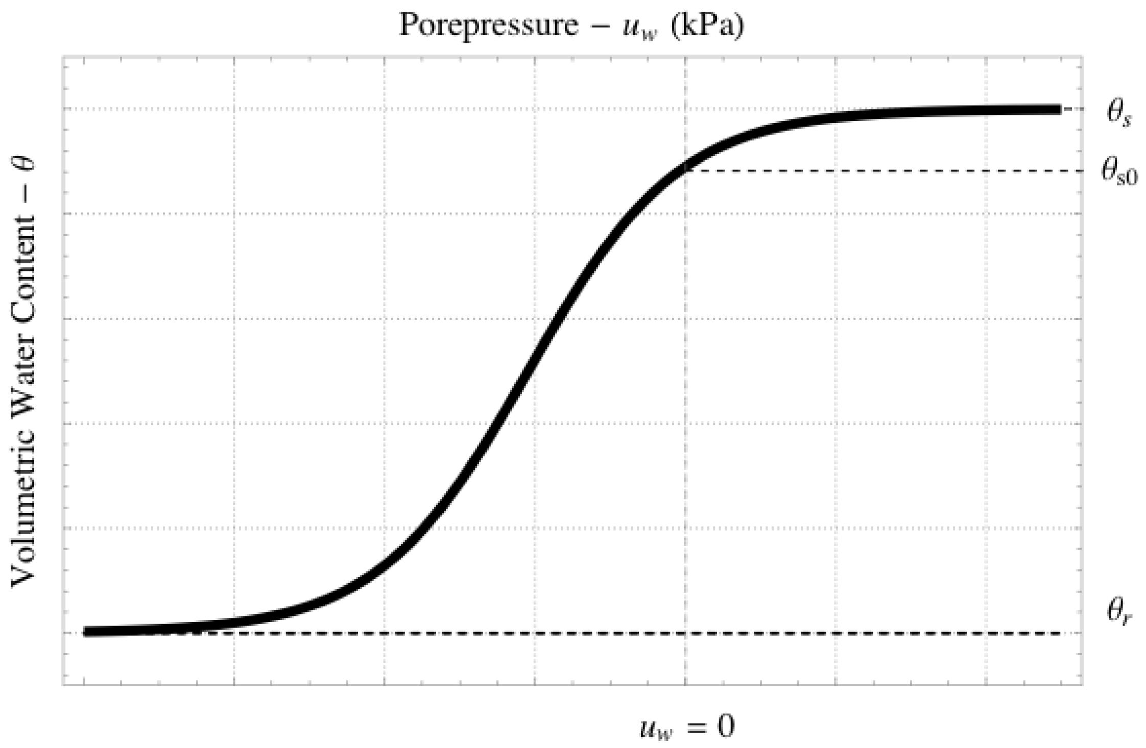
The SWRC expressed in Equation (4) is represented in Figure 1. It is important to discern that the saturation starting point ${\theta }_{s0}$ is different from the full saturation point ${\theta }_s$. As described in the second statement, the former is reached when the water occupies all the voids but the occluded bubbles, which are at atmospheric pressure. On the other hand, the latter can only be reached when the porepressure is so increased that the occluded bubbles are under a pressure that resizes them to a despicable volume. Furthermore, theoretically, the maximum volumetric water content (${\theta }_s$) can only be truly reached if one applies a porepressure that tends to infinity.

Equation (4) represents a unimodal soil, which means that there are only two asymptotes—the residual and the saturated volumetric water content. This may not be the case for all the soils, but it suffices for the theoretical explorations hereby carried out.

4. Normalized Water Content Solution

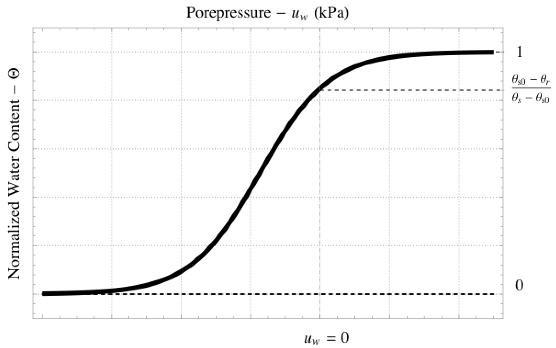
Equation (4) is a solution in terms of the volumetric water content; on the other hand, it is easy to rewrite such equation in terms of the normalized water content ($\Theta$), which can be expressed as:

$$\Theta =\frac{\theta -{\theta }_r}{{\theta }_s-{\theta }_r}$$

(6)

Hence, the derivative of Equation (6), in terms of porepressure, can be written as:

$$\frac{d\Theta }{d{u}_w}=\frac{1}{\left({\theta }_s-{\theta }_r\right)}\frac{d\theta }{d{u}_w}$$

(7)

or as:

$$\left({\theta }_s-{\theta }_r\right)\frac{d\Theta }{d{u}_w}=\frac{d\theta }{d{u}_w}$$

(8)

By combining Equations (3) and (8), one can find the following expression:

$$\left({\theta }_s-{\theta }_r\right)\frac{d\Theta }{d{u}_{{}_w}}={\delta }_1\left({\theta }_s-\theta \right)\left(\theta -{\theta }_r\right)$$

(9)

When dividing both sides of Equation (9) by $({\theta }_s-{\theta }_r)$, such equation can be written as follows:

$$\frac{d\Theta }{d{u}_w}={\delta }_1\left({\theta }_s-\theta \right)\Theta$$

(10)

Once more, dividing Equation (10) by $({\theta }_s-{\theta }_r)$, this equation can be rewritten as:

$$\frac{1}{\left({\theta }_s-{\theta }_r\right)}\frac{d\Theta }{d{u}_w}={\delta }_1\left(\frac{{\theta }_s-\theta }{{\theta }_s-{\theta }_r}\right)\Theta$$

(11)

or as,

$$\frac{1}{\left({\theta }_s-{\theta }_r\right)}\frac{d\Theta }{d{u}_w}={\delta }_1\left[\frac{\left({\theta }_s-{\theta }_r\right)-\left(\theta -{\theta }_r\right)}{\left({\theta }_s-{\theta }_r\right)}\right]\Theta$$

(12)

Thus, Equation (12) can be written as

$$\frac{d\Theta }{d{u}_w}={\delta }_1^{{}^{\prime }}\left[1-\Theta \right]\Theta$$

(13)

where ${\delta }_1^{\prime }$ is

$${\delta }_1^{{}^{\prime }}={\delta }_1\left({\theta }_s-{\theta }_r\right)$$

(14)

With the formulation presented in Equation (13), it is clear to notice that the differential equation that rules the relation between the normalized water content and porepressure is the same ODE that generates the logistic function. Therefore, by solving Equation (13) using the condition $\theta (u_w=0)={\theta }_{s0}$, one can find the following expression:

$$\Theta =\frac{1}{1+exp\left[-{\delta }_1^{{}^{\prime }}{u}_w-{\delta }_2\right]}$$

(15)

Similarly to Figure 1, it is possible to plot a qualitative analysis of the logistic function that represents the SWRC behavior. Therefore, Figure 2 shows the SWRC as predicted by Equation (15).

5. Experimental Exploratory Validation Analysis

The simple, intuitive description of the SWRC, hereby proposed through the two initial statements, is capable of generating ODEs and their respective solutions. However, to validate the suitability of the statements, one needs to check if the analytical solution is capable of modeling real experimental data.

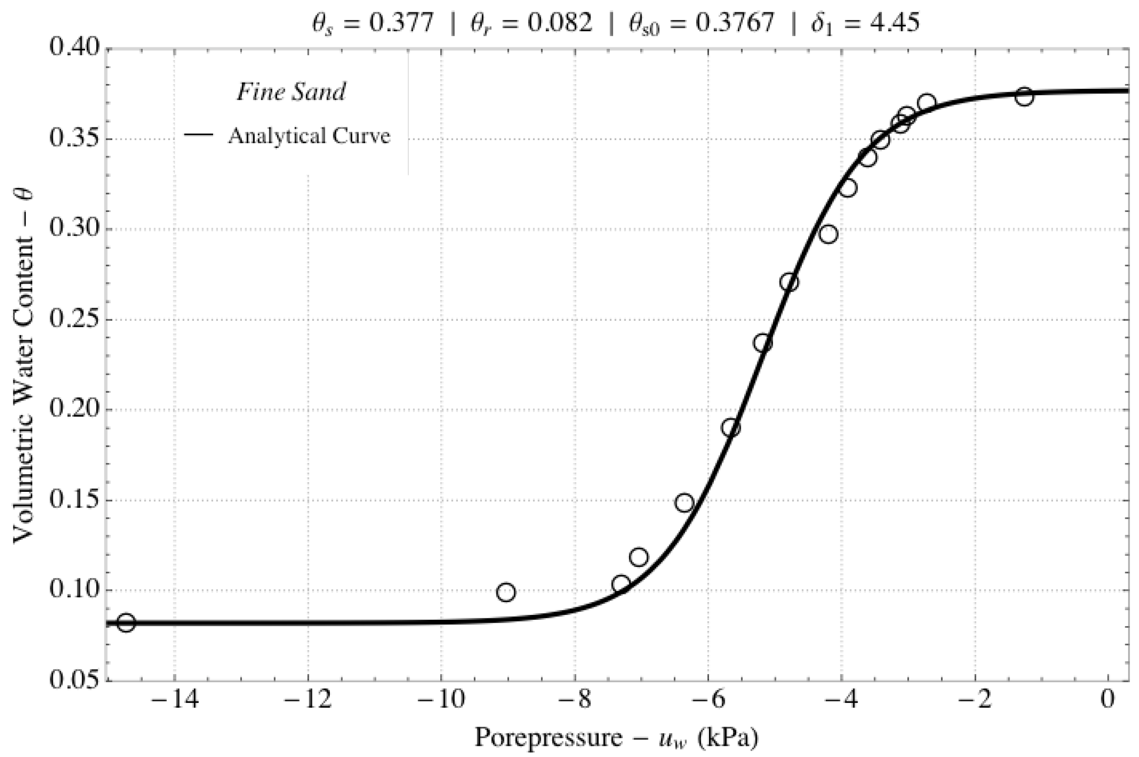
The purpose of Equation (4) is to model the behavior of both fine and coarse-grained unimodal soils. To check if the analytical expression can be used to model a coarse-grained soil, the dataset for the Fine Sand G.E.# 13 from Brooks and Corey [21] was chosen. Figure 3 shows the fitting of the analytical curve to the experimental data, highlighting the fitting parameters obtained. An extra point has been added to the dataset presented in [21] to indicate the porepressure close to saturation, i.e., the approximate intersection of the curve presented in the Brooks and Corey [21] article with their saturation line. This value was obtained graphically and corresponds to the point at −1.8 kPa of the porepressure in Figure 3.

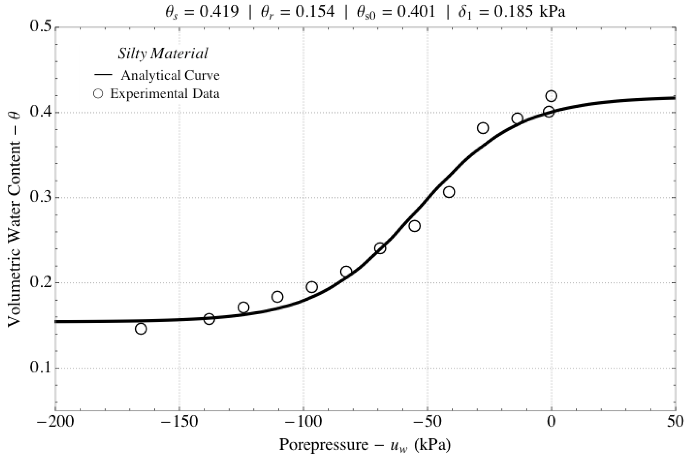
Moreover, the Silty Material from Aubertin et al. [22] was chosen to represent a fine soil. Similarly, Figure 4 shows the experimental data and the analytical curve with its fitting parameters.

As seen in Figure 3 and Figure 4, both analytical curves precisely fit the experimental data. Hence, for our exploratory analysis, the initial statements are plausible for describing the relation of porepressure and volumetric water content. It should be highlighted that further studies must be carried out to provide a robust validation of the modeling capabilities of this new SWRC. These studies, however, are not within the scope of the present study.

6. Numerical Approach

As demonstrated, the SWRC can be analytically formulated as a logistic function. Nevertheless, one could also numerically solve Equation (13) to find a discrete representation of the same logistic function.

6.1. Finite Difference Alternative

The Finite Difference Method (FDM) is capable of giving a precise solution to Equation (13). Thus, the discretization of Equation (13), in terms of forward differences, can be expressed as [23]:

$$\frac{{\Theta }_{n+1}-{\Theta }_n}{\Delta u_w}={\delta }_1^{{}^{\prime }}\left(1-{\Theta }_n\right){\Theta }_n$$

(16)

or as,

$${\Theta }_{n+1}=\Delta u_w\left[{\delta }_1^{{}^{\prime }}\left(1-{\Theta }_n\right){\Theta }_n\right]+{\Theta }_n$$

(17)

In order to use Equation (17), the numerical parameters that need to be chosen are the initial porepressure ($u_{w0}$), the porepressure step ($\Delta u_w$) and the hydraulic parameter (${\delta }_1^{{}^{\prime }}$). One may notice that the soil type (either fine or coarse-grained) does not interfere with the numerical suitability of the FDM solution. If one defines a small enough porepressure step, the numerical solution can be as precise as desired. One lacks, on the other hand, a precise definition of the stability and convergence of the FDM scheme used. This will be explored in the next section.

6.2. Beyond the Numerical Approach: Logistic Map Attractor

The discrete counterpart of Equation (15) given in Equation (17) brings interesting properties that may not be directly linked to the new SWRC. Even though it has not been fully explored how the new formulation can be used to model multiple soil types, it has been shown that at least some types will be satisfactorily modeled. This implies that Equation (17), within ranges where the solution is stable and convergent, may be considered a true model of a SWRC.

On the other hand, one may notice that the discrete equation represented in Equation (17) is a form of the logistic equation. Logistic equations are nonlinear recurrence relations that describe sigmoid patterns. In order to make this correlation clearer, Equation (17) can be rearranged to resemble the usual logistic map recurrence equation as:

$${\Omega }_{n+1}=(1+\Delta u_w{\delta }_1^{{}^{\prime }})\left(1-{\Omega }_n\right){\Omega }_n$$

(18)

where ${\Omega }_n={\Theta }_n\Delta u_w{\delta }_1^{{}^{\prime }}/\phantom{{\Theta }_n\Delta u_w{\delta }_1^{{}^{\prime }}(1+\Delta u_w{\delta }_1^{{}^{\prime }})}(1+\Delta u_w{\delta }_1^{{}^{\prime }})$. It can be seen that $0\le {\Omega }_n\le 1$ and that the parameter of the logistic map is $(1+\Delta u_w{\delta }_1^{{}^{\prime }})$. If one plots the normalized water content ($\Theta$) versus the product of ${\delta }_1^{{}^{\prime }}$ and the porepressure step ($\Delta u_w$), it is possible to find an interesting pattern, as seen in Figure 5.

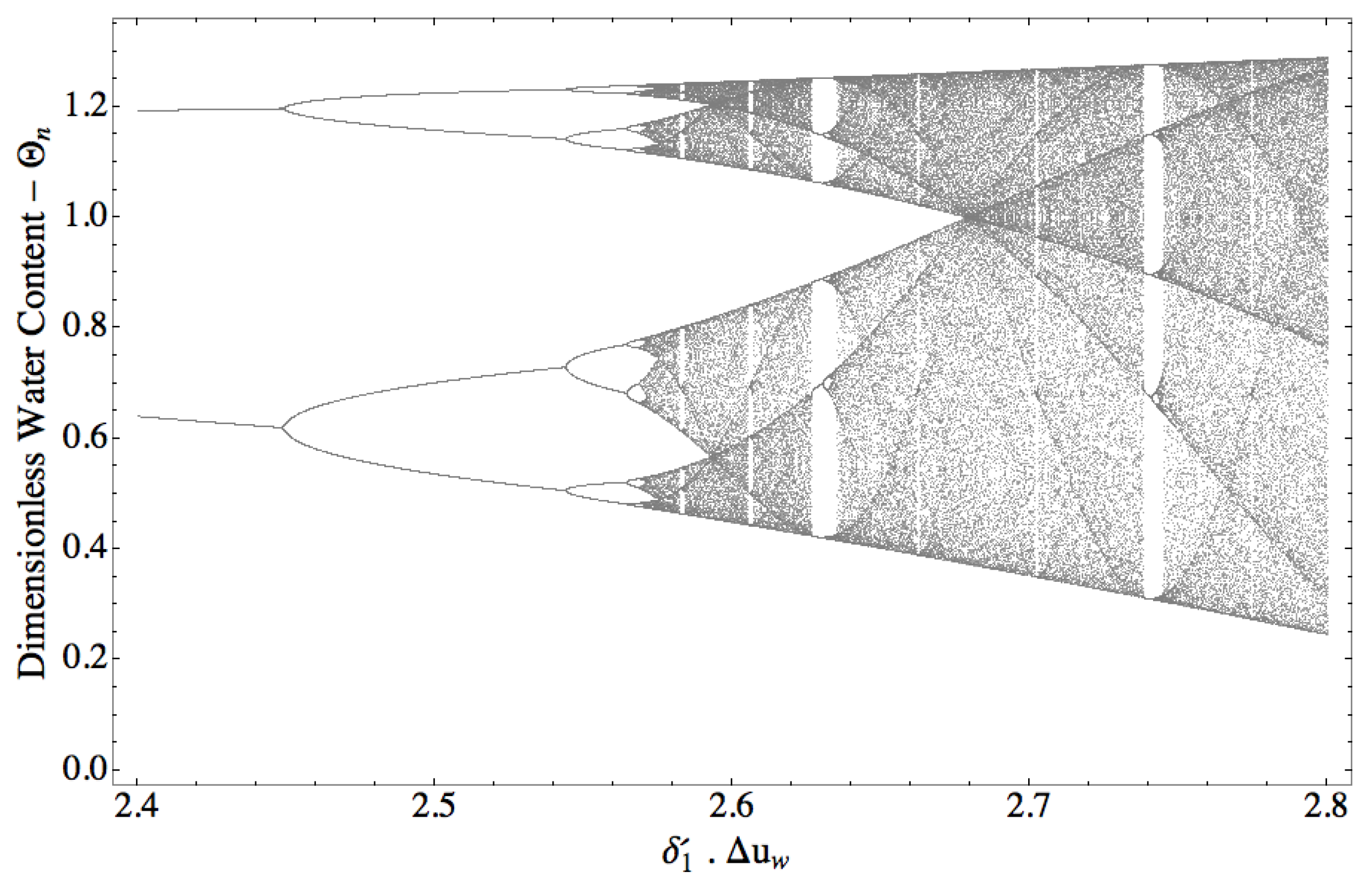
Figure 5 is called the bifurcation diagram for the logistic map. When the value of ${\delta }_1^{{}^{\prime }}\Delta u_w$ is close to 2, the bifurcation occurs. In the bifurcation, the logistic map presents a wave pattern with a single oscillation range. Just a little after 2.4, there is another bifurcation. This new bifurcation now allows the curve to present two ranges of oscillation. After that, many other bifurcations occur, leading the curve to a chaotic pattern. However, if one takes a closer look at the bifurcation diagram, as presented in Figure 6, it is possible to see that the bifurcation pattern is self-similar. Actually, it behaves as a fractal and has its boundaries well determined, even though the scattering may be difficult to define.

It must be highlighted that the logistic map parameter is $(1+\Delta u_w{\delta }_1^{{}^{\prime }})$. If $\Delta u_w{\delta }_1^{{}^{\prime }}$ is sufficiently small, the numerical solution obtained by the FDM converges to the analytical solution. However, if one considers greater values for $\Delta u_w{\delta }_1^{{}^{\prime }}$, the change in the logistic map parameter indicates that the link to the FDM solution may be lost, leading to divergent (apparently chaotic) results.

This parameter range can be used as a proxy for the adequacy of the FDM representation of the new SWRC. If the parameters’ product falls outside the pre-bifurcation interval, this indicates that the link between the continuous SWRC and its discrete approximation may not be present anymore. By now, it is important to highlight that the logistic map can be used, upon restrictions, to model the new SWRC. The possibility of extending the validity of the logistic map modeling after bifurcation to the new SWRC will be studied in subsequent papers in detail. Previous results [15,16], however, indicated that there exists a relation between discrete and continuous phenomena in geotechnical engineering.

7. Conclusions

First, based on simple assertions, mathematical statements were postulated and then combined into an ODE. In addition, the ODE was solved, and a simple model for the SWRC expression was found to follow a logistic function. By using real experimental results from both fine and coarse-grained soils, it was shown that, in a first exploratory analysis, the proposed SWRC may be suitable for modeling specific fine and coarse-grained soils. Further studies analyzing the modeling capabilities of the new SWRC to other types of soils still need to be carried out and will be the focus of future works.

Usually, SWRCs are obtained more through a mathematical fitting point of view rather than an algebraic deduction from simple physical principles. Thus, a relevant contribution of the present paper is the overview of an interesting yet simple physical foundation for the nature of soil–water relations.

Moreover, the concepts of initial saturation and total saturation were introduced. These concepts allowed the authors to describe the SWRC for both unsaturated and saturated flow in a smooth and continuous approach. Thus, using this new curve made it possible, along with the continuity equation and the other necessary constitutive models, to simulate both unsaturated and saturated in the same mathematical domain. It is believed that this better represents the nature of the wetting/drying of samples, as both saturated and unsaturated flows share boundaries in many cases.

Furthermore, it was demonstrated that a discrete modeling of the SWRC as a logistic map brings important considerations about the convergence and stability of the FDM scheme used. Furthermore, one can conclude from the logistic map point of view that chaos is just a matter of scale. The complexity of a system, which may drastically vary according to its initial conditions, can also present order. It is true, indeed, that the oscillation ranges are hard to define on the discrete representation of the SWRC after it apparently diverges. However, the logistic map shows a fractal relation for the boundaries of the oscillation range of these curves.

The next studies on this topic may address other important issues. In addition to experimentally validating the new SWRC, the most relevant one seems to be understanding how the logistic map could be linked to the SWRC after bifurcation occurs.

References

- Fredlund, D.; Rahardjo, H. Soil Mechanics for Unsatured Soils; John Wiley & Sons: New York, NY, USA, 1993; Volume 24. [Google Scholar] [CrossRef]
- van Genuchten, M.T. A Closed-form Equation for Predicting the Hydraulic Conductivity of Unsaturated Soils. Soil Sci. Soc. Am. J. 1980, 44, 892–898. [Google Scholar] [CrossRef] [Green Version]
- Fredlund, D.G.; Xing, A. Equations for the soil-water characteristic curve. Can. Geotech. J. 1994, 31, 521–532. [Google Scholar] [CrossRef]
- Cavalcante, A.L.B.; Zornberg, J.G. Efficient Approach to Solving Transient Unsaturated Flow Problems. I: Analytical Solutions. Int. J. Geomech. 2017, 17, 04017013. [Google Scholar] [CrossRef] [Green Version]
- Cavalcante, A.L.B.; Zornberg, J.G. Efficient Approach to Solving Transient Unsaturated Flow Problems. II: Numerical Solutions. Int. J. Geomech. 2017, 17, 04017014. [Google Scholar] [CrossRef]
- Haverkamp, R.; Parlange, J.Y. Predicting the water-retention curve from particle-size distribution. Soil Sci. 1986, 142, 325–339. [Google Scholar] [CrossRef]
- Turturro, A.C.; Caputo, M.C.; Gerke, H.H. Mercury intrusion porosimetry and centrifuge methods for extended-range retention curves of soil and porous rock samples. Vadose Zone J. 2022, 21, e20176. [Google Scholar] [CrossRef]
- Du, C. Comparison of the performance of 22 models describing soil water retention curves from saturation to oven dryness. Vadose Zone J. 2020, 19, e20072. [Google Scholar] [CrossRef]
- Klein, M.J. Max Planck and the Beginnings of the Quantum Theory. Arch. Hist. Exact Sci. 1962, 1, 459–479. [Google Scholar] [CrossRef]
- Hooft, G. Quantization of point particles in (2 + 1)-dimensional gravity and spacetime discreteness. Class. Quantum Gravity 1996, 13, 1023–1039. [Google Scholar] [CrossRef] [Green Version]
- Ali, A.F.; Das, S.; Vagenas, E.C. Discreteness of space from the generalized uncertainty principle. Phys. Lett. B 2009, 678, 497–499. [Google Scholar] [CrossRef] [Green Version]
- Riek, R. A Derivation of a Microscopic Entropy and Time Irreversibility from the Discreteness of Time. Entropy 2014, 16, 3149–3172. [Google Scholar] [CrossRef] [Green Version]
- Wolfram, S. A New Kind of Science; Wolfram Media Inc.: Champaign, IL, USA, 2002. [Google Scholar]
- Wolfram, S. Theory and Applications of Cellular Automata; World Scientific: Singapore, 1986. [Google Scholar]
- Ozelim, L.C.S.M.; Cavalcante, A.L.B.; Borges, L.P.F. Continuum versus Discrete: A Physically Interpretable General Rule for Cellular Automata By Means of Modular Arithmetic. Complex Syst. 2013, 22, 75–99. [Google Scholar]
- Ozelim, L.C.S.M.; Cavalcante, A.L.B.; Baetens, J.M. On the iota-delta function: A link between cellular automata and partial differential equations for modeling advection–dispersion from a constant source. J. Supercomput. 2017, 73, 700–712. [Google Scholar] [CrossRef]
- Othmer, H.; Diekkruger, B.; Kutilek, M. Bimodal Porosity and Unsaturated Hydraulic Conductivity. Soil Sci. 1991, 152, 139–150. [Google Scholar] [CrossRef]
- Gitirana, G.d.F.N.; Fredlund, D.G. Soil-Water Characteristic Curve Equation with Independent Properties. J. Geotech. Geoenviron. Eng. 2004, 130, 209–212. [Google Scholar] [CrossRef]
- Costa, M.B.A.d.; Cavalcante, A.L.B. Bimodal Soil-Water Retention Curve and k-Function Model Using Linear Superposition. Int. J. Geomech. 2021, 21, 04021116. [Google Scholar] [CrossRef]
- Groenevelt, P.H.; Grant, C.D. A new model for the soil-water retention curve that solves the problem of residual water contents. Eur. J. Soil Sci. 2004, 55, 479–485. [Google Scholar] [CrossRef]
- Brooks, R.H.; Corey, A.T. Hydraulic Properties of Porous Media; Colorado State University Hydrology Paper; Colorado State University: Fort Collins, CO, USA, 1964. [Google Scholar]
- Aubertin, M.; Mbonimpa, M.; Bussière, B.; Chapuis, R.P. A model to predict the water retention curve from basic geotechnical properties. Can. Geotech. J. 2003, 40, 1104–1122. [Google Scholar] [CrossRef]
- Courant, R. Differential and Integral Calculus; Wiley Classics Library, Wiley: New York, NY, USA, 1988; Volume 1. [Google Scholar]
Figure 1.
Qualitative description of the volumetric water content curve.
Figure 2.
Qualitative description of the normalized water content.
Figure 3.
Analytical fitting for the fine Sand G.E. # 13 from Brooks and Corey [21].
Figure 4.
Analytical fitting for the silty material from Aubertin et al. [22].
Figure 5.
Logistic map of the SWRC discrete equation.
Figure 6.
Magnification of the logistic map of the SWRC.
Publisher’s Note: MDPI stays neutral with regard to jurisdictional claims in published maps and institutional affiliations. |
© 2022 by the authors. Licensee MDPI, Basel, Switzerland. This article is an open access article distributed under the terms and conditions of the Creative Commons Attribution (CC BY) license (https://creativecommons.org/licenses/by/4.0/).
Share and Cite
MDPI and ACS Style
Borges, L.P.d.F.; Cavalcante, A.L.B.; Ozelim, L.C.d.S.M. Order Out of Chaos in Soil–Water Retention Curves. Water 2022, 14, 2421. https://doi.org/10.3390/w14152421
AMA Style
Borges LPdF, Cavalcante ALB, Ozelim LCdSM. Order Out of Chaos in Soil–Water Retention Curves. Water. 2022; 14(15):2421. https://doi.org/10.3390/w14152421
Chicago/Turabian StyleBorges, Lucas Parreira de Faria, André Luís Brasil Cavalcante, and Luan Carlos de Sena Monteiro Ozelim. 2022. "Order Out of Chaos in Soil–Water Retention Curves" Water 14, no. 15: 2421. https://doi.org/10.3390/w14152421
Note that from the first issue of 2016, this journal uses article numbers instead of page numbers. See further details here.