
A Machine Learning-Based Surrogate Model for the Identification of Risk Zones Due to Off-Stream Reservoir Failure


1
International Centre for Numerical Methods in Engineering (CIMNE), 08034 Barcelona, Spain
2
Flumen Institute, Universitat Politècnica de Catalunya (UPC BarcelonaTech)—International Centre for Numerical Methods in Engineering (CIMNE), 08034 Barcelona, Spain
*
Author to whom correspondence should be addressed.
Water 2022, 14(15), 2416; https://doi.org/10.3390/w14152416
Submission received: 27 June 2022
/
Revised: 21 July 2022
/
Accepted: 27 July 2022
/
Published: 4 August 2022
(This article belongs to the Section Water Resources Management, Policy and Governance)
Abstract
:Approximately 70,000 Spanish off-stream reservoirs, many of them irrigation ponds, need to be evaluated in terms of their potential hazard to comply with the new national Regulation of the Hydraulic Public Domain. This requires a great engineering effort to evaluate different scenarios with two-dimensional hydraulic models, for which many owners lack the necessary resources. This work presents a simplified methodology based on machine learning to identify risk zones at any point in the vicinity of an off-stream reservoir without the need to elaborate and run full two-dimensional hydraulic models. A predictive model based on random forest was created from datasets including the results of synthetic cases computed with an automatic tool based on the two-dimensional numerical software Iber. Once fitted, the model provided an estimate on the potential hazard considering the physical characteristics of the structure, the surrounding terrain and the vulnerable locations. Two approaches were compared for balancing the dataset: the synthetic minority oversampling and the random undersampling. Results from the random forest model adjusted with the random undersampling technique showed to be useful for the estimation of risk zones. On a real application test the simplified method achieved 91% accuracy.
Keywords:
machine learning; Iber; off-stream reservoirs; dam breach; floods; random forest; surrogate model1. Introduction
Off-stream reservoirs are essential structures for the regulation and supply of water. In contrast to dams, they are not usually affected by surface runoff, which results in higher hydrological safety. Nonetheless, many of these structures are located in high elevations, near to urban areas and important infrastructure that can be affected in case of failure.
With the modification of the Spanish Regulation of the Hydraulic Public Domain derived from the Royal Decree 9/2008 [1], the potential hazard of off-stream reservoirs higher than 5 m or with volume storage above 100,000 m3 must be evaluated with the same procedure as for large dams (higher than 15 m or with more than 100,000 m3 of capacity). This means that around 70,000 off-stream reservoirs currently in operation in Spain [2] need to be assessed on the potential hazard due to failure.
The Spanish Technical Guide for dam classification based on potential hazard [3], hereinafter the “Technical Guide”, lists the recommended methods to analyse the dam breach formation and flood propagation. Three categories are described in the Technical Guide, namely A, B and C, from higher to lower potential hazard. The classification process involves two main steps: (a) identification of the relevant elements potentially affected (e.g., households, roads) and (b) generation of the flood maps. This is generally performed through the application of two-dimensional (2D) hydraulic models that consider the hydraulic characteristics of the flow propagation downstream of the dam breach and provide results in terms of maximum depths and velocities, allowing for the identification of the flooded area [4].
The complete method, which involves hydraulic 2D models, is recommended to reproduce the breach formation, the failure hydrograph and the flood propagation. Currently, different software tools meet the requirements of this method, such as the National Weather Service Dam-break Flood Forecasting Model (NWS DAMBRK) [5], the Simplified Dam-Break model (SMPDBK) [6], and Iber [7], among others [4]. The results of the hydraulic model are the basis for evaluating the affections to the zones of interest. Simplified methods are also accepted if the classification of the structure is obvious.
The necessary work to make a complete and accurate classification assessment of the potential hazard requires engineering knowledge and resources often unavailable for many owners. In addition, the administration responsible for the review and approval of the classification assessments and emergency plans requires relevant time and human resources.
Despite the increasing growth in the exploitation of off-stream reservoirs and the need for safety analyses, few studies have been published on their potential hazard. Soler et al. [8] analysed the effect of using 1D or 2D models for flood propagation in case of failure. Two-dimensional models were more accurate for the simulation of free surface flows, allowing for a better classification of the structure. Espejo [9] characterized the hydraulics of off-stream reservoir failures by defining the storage factor to facilitate the selection of the empirical formulas for computing breach parameters (width and formation time). Hence, the hydraulic operation regarding the breaching of the off-stream reservoir is projected based on the height and volume of the reservoir, in terms of the probability of occurrence of a specific flow discharge. Additionally, a cartographic representation of the areas most likely to be affected was created using 5000 simulations of synthetic scenarios and stochastic analysis (Monte Carlo approach). Hori et al. [10] developed a disaster prevention support system for irrigation ponds in Japan after the failure of many off-stream reservoirs due to an earthquake in 2011. The system allows for determining the risk in heavy rain scenarios and calculating inundation areas in case of failure. Sánchez-Romero et al. [11] explained in detail the process of generating flood maps due to the failure of off-stream reservoirs using FLDWAV and Iber for two piping and overtopping. The results showed smaller peak flows in overtopping failure, although the discharge volumes are larger than those produced by piping.
The development of simplified tools for analysing the consequences of dam breach has been a topic of increasing interest in the last years. Different methodologies have been proposed, most of which are based on Geographic Information System (GIS) tools. Cannata and Marzocchi [12] developed a GIS-embedded approach to derive maximum flooding maps based on elevation raster maps. The tool solves the 2D shallow-water equations using a finite volume method and achieved 75% accuracy as compared to the official flooding map of an existing dam. In addition, Albano et al. [13] implemented a GIS-based method to delineate flood-prone areas in case of dam break. A set of cross-sections are created over a digital elevation model (DEM) along the downstream river reach, and the maximum discharge, elevation and time are computed with a 1D unsteady flow solver. The tool achieved an accuracy of 86% with respect to maps generated with a 2D model.
In parallel, some authors applied machine learning (ML) techniques for simplifying dam breaching and dam safety analysis. Hooshyaripor et al. [14] proposed an artificial neural network model (ANN) to predict the peak discharge due to breaching of embankment dams using a dataset with 93 failures. The results showed that the method is not applicable for peak outflows lower than 100 m3/s due to the small size of the dataset. In another study, Hooshyaripor et al. [15] reported higher accuracy on a synthetic dataset generated by means of copulas based on the independent relationship between height and volume of water in the reservoirs. ML algorithms have also been applied to other dam safety problems, such as the prediction of dam behaviour [16,17], the detection of anomalies [18,19,20] based on monitoring data, or the prediction of flood maps [21,22].
The aim of this work is to present a methodology based on ML to estimate the potential affection in case of failure of an off-stream reservoir on any location in the surrounding area without the need of running a detailed 2D hydraulic model. The information required includes 10 parameters related to the geometry of the reservoir, the roughness and slope of the terrain and the relative location of the potentially affected elements. The required—large—dataset to fit the model is created with the results of synthetic cases generated using a tool based on Iber [7,23] and Latin Hypercube Sampling (LHS) [24].
The paper is organised as follows: first, the methods used are explained in Section 2, including the automated generation and parametrization of synthetic cases for construction of the database, the ML algorithms, and their calibration and validation; results are presented in Section 3; application to a real case is shown in Section 4. Section 5 includes the discussion, while conclusions are summarized in Section 6.
2. Methods
The ML models were fitted using synthetic data generated by means of complete 2D hydraulic models developed in Iber. The steps included in the overall workflow are:
- Parametrization of the physical variables of the structure and the surrounding terrain.
- Design and generation of synthetic cases.
- Automation of Iber for computing breach formation and flood propagation and for extracting the results of each synthetic case.
- Generation of the dataset and classification of the results based on the criteria established in the Spanish Regulation [1].
- Training, calibration and performance assessment of a ML classification model.
- Validation of the ML model and analysis of the results.
2.1. Data Generation
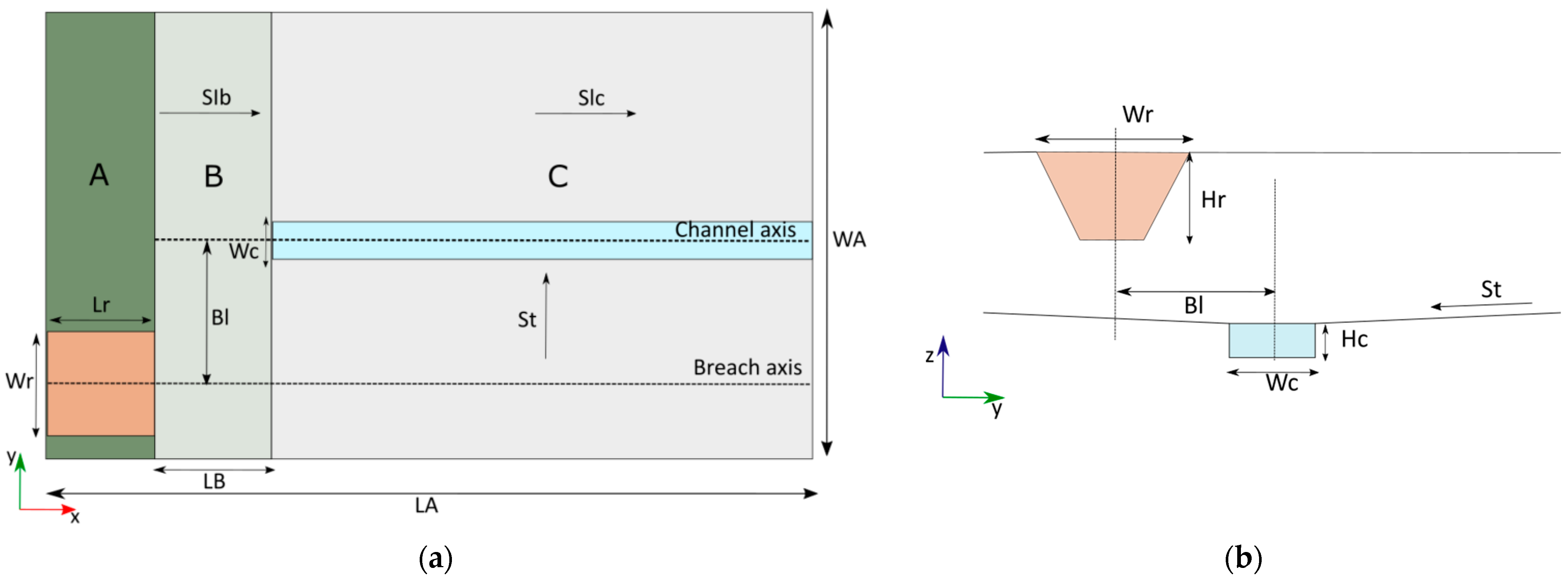
The synthetic cases were defined based on ten parameters shown in Figure 1. The length of the domain is 4000 m (LA), and the width is 1500 m (WA), with three sections: A, B and C (Figure 1a). The default maximum top elevation (Et) is 505 m for all cases. The off-stream reservoir is located in Section A (brown area) and has the highest elevation. The location of the off-stream reservoir can vary along the y-axis. Section B represents a transition zone between the off-stream reservoir and section C with a longitudinal slope (SlB) between 0% and 1% and no transversal slope. In section C, a main channel is assumed to exist at the origin of the y-axis (y = 0) with a rectangular shape (cyan area). The area outside the channel has a given constant transversal slope (St) leading the flow into the channel.
Table 1 shows the parameters with their symbols and ranges of variation. For cases without a defined channel (Wc = 0), the geometry was designed to convey the water flow towards the centre of the terrain based on the transversal slope in section C.
A design of experiment (DoE) technique based on Latin hypercube sampling (LHS) was applied for generating the combination of parameters for each synthetic case. LHS is a statistical method for sampling that ensures that the distribution of each input parameter is fully represented using all areas of the sample space. LHS allows fewer simulations to be performed while obtaining similar precision and lower variance than other methods such as random sampling, which does not take into account the previously generated sample points [24,25].
Two sets of samples were generated with LHS. In the first 50 samples, no main channel was defined, i.e., Hc = 0 and Wc = 0. This dataset accounts for cases in which no clear flow path exists in the vicinity of the off-stream reservoir. In the other 150 samples, all parameters were equally sampled along their range of variation, always using uniform distributions.
For each combination of parameters, the geometry was generated by means of a list of points with xyz coordinates. In section A, the separation between points is from 5 to 40 m in the x-axis, depending on the length of the off-stream reservoir, and 5 m in the y-axis. For sections B and C, the separation is 20 m for both axes, except on the main channel, where the separation is 0.5 m in the y-axis. For section A, the off-stream reservoir needed more detail for the estimation of the breach.
The breach is placed at half the width of the reservoir and starts at the crest. The storage volume in the reservoir is approximated using the volume equation of a trapezoidal prism with Hr, Wr and Lr dimensions.
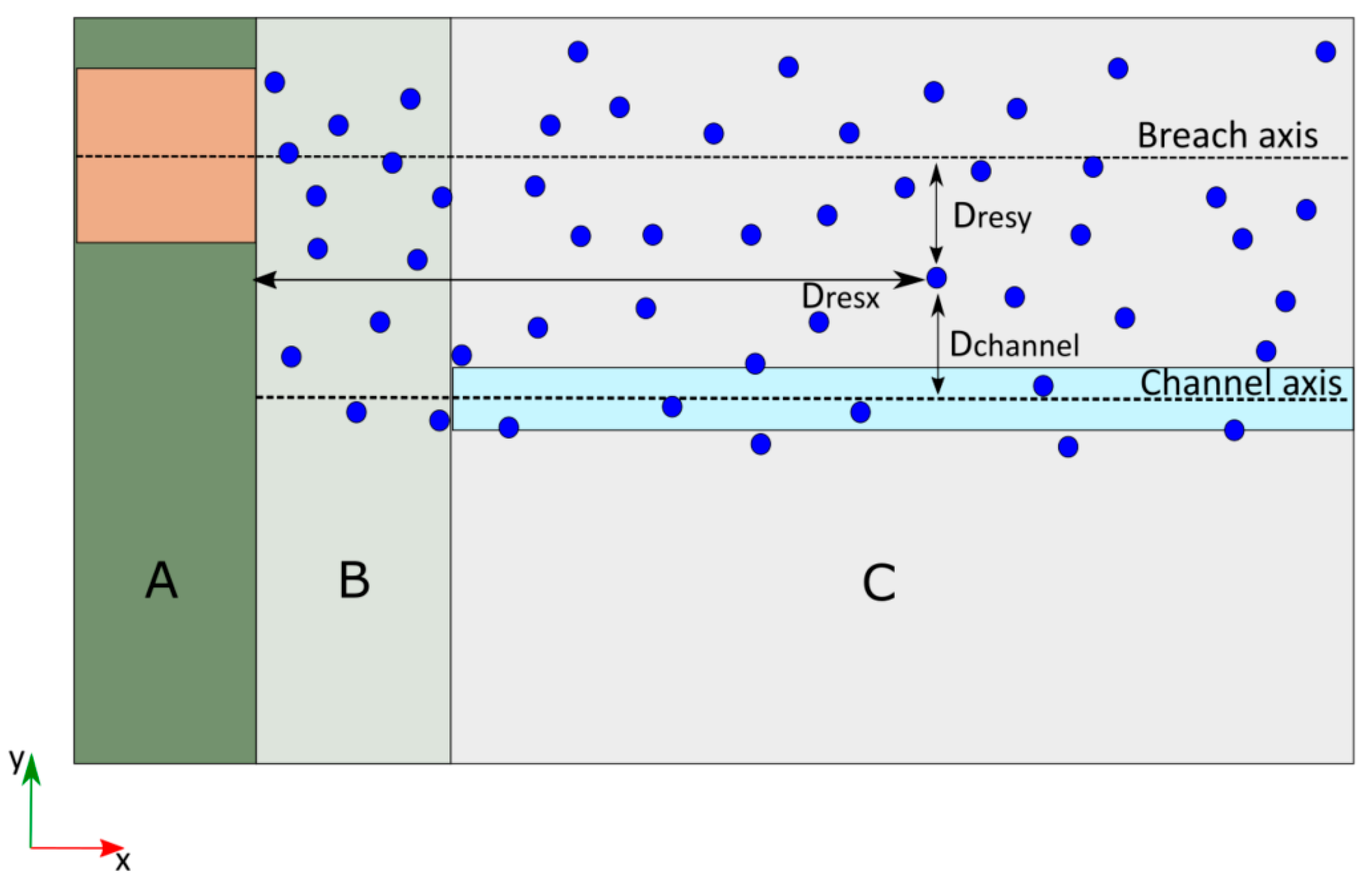
For the extraction of results, 200 points (or gauges) were considered for each case as vulnerable locations. They are situated at random in the area where the flood is expected to affect, i.e., close to the reservoir, the breach axis and the channel axis. More precisely, the location of the gauges was parametrized on the basis of three variables (Figure 2). Dresx is the distance to the off-stream reservoir embankment (location of the breach) along the x-axis, Dresy is the distance to the breach axis, and Dchannely is the distance to the main channel axis. The values for Dresy and Dchannely vary from −750 to 750 and for Dresx from 60 to 3950.
2.2. Automation in Iber
Iber is a 2D numerical tool for modelling hydrodynamic and sediment transport [7,23], which currently includes additional calculation modules for simulating hydrological processes [26,27], pollutant propagation [28], large-wood transport [29], physical habitat suitability assessment [30] and dam and off-stream reservoir breach formation [31,32,33]. Iber uses the finite volume method to solve the 2D depth average shallow water equations and is integrated in the pre- and post-processing interface of GiD, a software for definition, meshing and results visualization of numerical models [31,34]. Additionally, Iber calculations can be accelerated using graphical processing units (GPUs) [35].
A tool in Iber was developed to automate the process of model generation and results extraction. With this tool, the information regarding the geometry, breach parameters and gauges for each synthetic case is read, and the roughness of the model is assigned. Six land use types were considered: 0.020, 0.025, 0.032, 0.050, 0.080 and 0.120 s/m1/3. Each synthetic case is computed with six different Manning coefficients, resulting in 1200 models (200 × 6). Then, the mesh is generated, the models are run and the results exported in CSV format: depth (h), specific discharge in x (qx) and specific discharge in y (qy) every 300 s for each gauge.
The total calculation time was set at 16,000 s. It was obtained from an estimated average velocity of 0.25 m/s to ensure that the flood wave propagation over the entire area is computed.
2.3. Definition of Hazard
The Spanish Regulation 9/2008 in its article 9 (2) states that a hazard to human life is considered to exist when the depth of water is 1 m or more, the velocity is 1 m/s or more, or the product of depth and velocity is 0.5 m2/s or more [1]. Therefore, two classes were defined: class 0 when none of the three criteria are met and class 1 when one or more criteria are true.
2.4. Machine Learning
The main goal of ML models is to reproduce the response of a system for unseen scenarios based on patterns previously identified from a typically large database (training set). The accuracy of an ML model is typically evaluated on a dataset not used for model fitting (test set).
There are two types of ML supervised models according to the type of output. Numerical responses are predicted with regression, while categorical outcomes are estimated with classification models.
In this work, supervised classification models were used, because the output is categorical (class 0 or class 1 as described in Section 2.3). Among the available ML classification algorithms, random forests (RF) was chosen for this work because: (a) it showed to be useful and easy to implement in previous works [19,36]; (b) it outperformed other classification algorithms in a comprehensive comparative analysis [37,38]; (c) the application of RF models has increased in water engineering due to their high accuracy, flexibility and possibilities for interpretation [37,38,39].
2.4.1. Random Forest
An RF model is a combination of a large number of decision trees, each of which is bootstrapped to a random sample taken from the training set. The bootstrapping involves resampling the data with replacements, eliminating some of the samples and duplicating others. Then, each decision tree is fitted with a different sample. The RF method introduces additional randomness by taking a random subset of the input variables when computing each split for each tree in the model. The final prediction of the algorithm is calculated based on the average of the results of each of the trees used. A detailed description of the algorithm can be found in the seminal work of Breiman [40]. For more practical descriptions of the method, the reader can consult [41,42].
In this work, the scikit-learn package developed for Python was used, which includes the random forests classifier option [43]. The main parameters to build an RF model are the number of trees to be ensembled (n_estimators), the minimum number of samples required to split an internal node (min_sample_split) and the maximum number of features considered for each tree (max_features).
2.4.2. Balanced Dataset
Imbalance datasets are reported as a major problem to the development of accurate ML classifiers algorithms [44]. Our training set is imbalanced because one class (class 0) heavily outnumbers the samples from the other class (class 1). Among the available methods for alleviating this problem, we tried under- and oversampling methods: synthetic minority oversampling technique (SMOTE) [45] and random undersampling (RUS) [46].
SMOTE is a combination of oversampling of the minority class and undersampling of the majority class. New synthetic examples based on the characteristics of the existing data are created using interpolation with the k-nearest neighbour technique. With RUS, samples corresponding to the predominant class are eliminated, and no new information is introduced. Thus, the majority class is reduced to the same amount of samples corresponding to the minority class [44].
2.4.3. Calibration Procedure
The observations excluded from a bootstrap sample are called out-of-bag data (OOB). The OOB predictions are calculated only using the trees for which the observations are OOB [47]. The OOB error is calculated as the average of the OOB error rate for each observation. This procedure can be considered as implicit cross-validation, which can obtain a good estimate of the prediction error without the need to explicitly separate a subset of the available data [48].
A calibration process was performed based on the OOB error rate to find the best combination of parameters for the RF model. The OOB error rate was estimated for different possible combinations of the model parameters, and the best combination (lowest OOB error) was selected to fit the final RF model. All possible combinations of n_estimators (600, 800, 1000 and 1200), min_sample_split (2, 3 and 5) and max_features (3, 4, 5 and 6) were considered to fit the RF models.
2.4.4. Measures of Accuracy
Henceforth, the correct estimation of class 1 is considered as positive experiments (true positives, ), while the correct prediction of class 0 corresponds to negative experiments (true negatives, ). False positives () are cases where the model predicts a risk to human life in an unaffected area, and false negatives () are those for which the model predicts no risk in areas with true damage [49]. The measures of accuracy considered are:
The adjusted F-score can place higher importance on the precision or recall according to the nature of the study. Since false negatives are more relevant in our problem, recall is considered more important, and the F2 score is estimated with the generalized -score formula with = 2 [50].
The receiver operating characteristic (ROC) curve is a useful tool to visualize the performance of binary classifier algorithms. Plotting the against the false positive rate (FPR) generates the ROC curve [46]. The area under the ROC curve (AUC) is an additional measure for evaluating the predictive ability of classifiers [51]. Values of AUC close to one represent a good classifier, while the model is not able to distinguish between classes when AUC is equal to 0.5.
3. Results
3.1. Data Preparation
The training set includes 150 of the 200 available geometries (75%), taken at random. The remaining 50 (25%) are kept for the test set. Additionally, the results from 20 synthetic models not included in the training or testing set, each one with six different land uses, formed a validation dataset (120 models).
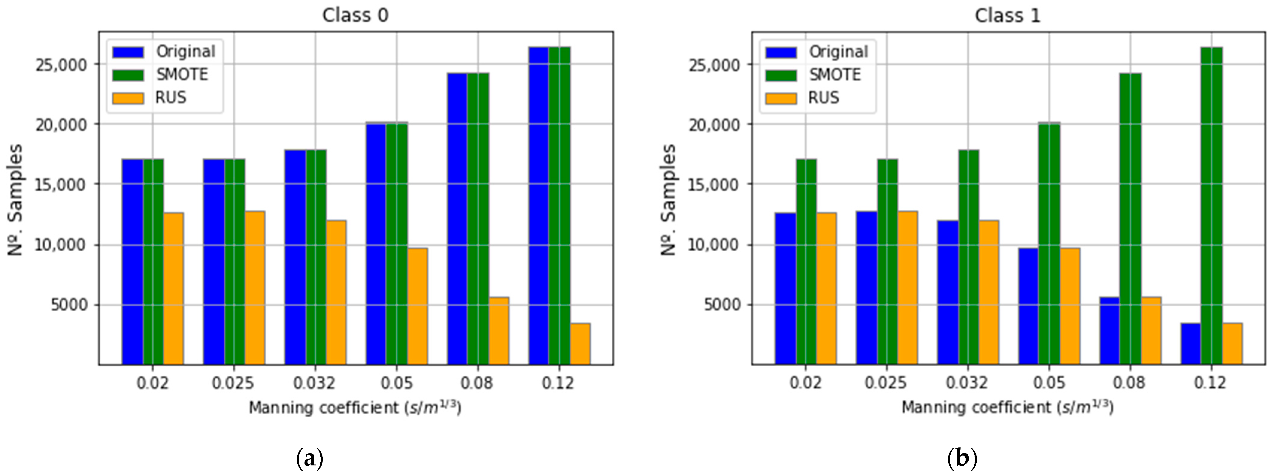
In the training set, 62% of the samples belong to class 0 and 38% for class 1. In addition, the ratio of class 1 samples decreases as the Manning coefficient increases (Table 2).
Therefore, each subset of the training data, segregated by the Manning coefficient, was balanced with two methods (SMOTE and RUS) to ensure that the RF model can predict with high accuracy both categories. Figure 3 presents the distribution of the classes before and after balancing the subsets with both methods. Hereafter, “RF-OS” stands for the RF model fitted with the dataset balanced with SMOTE and “RF-US” for the model fitted with the dataset balanced with RUS.
3.2. Calibration
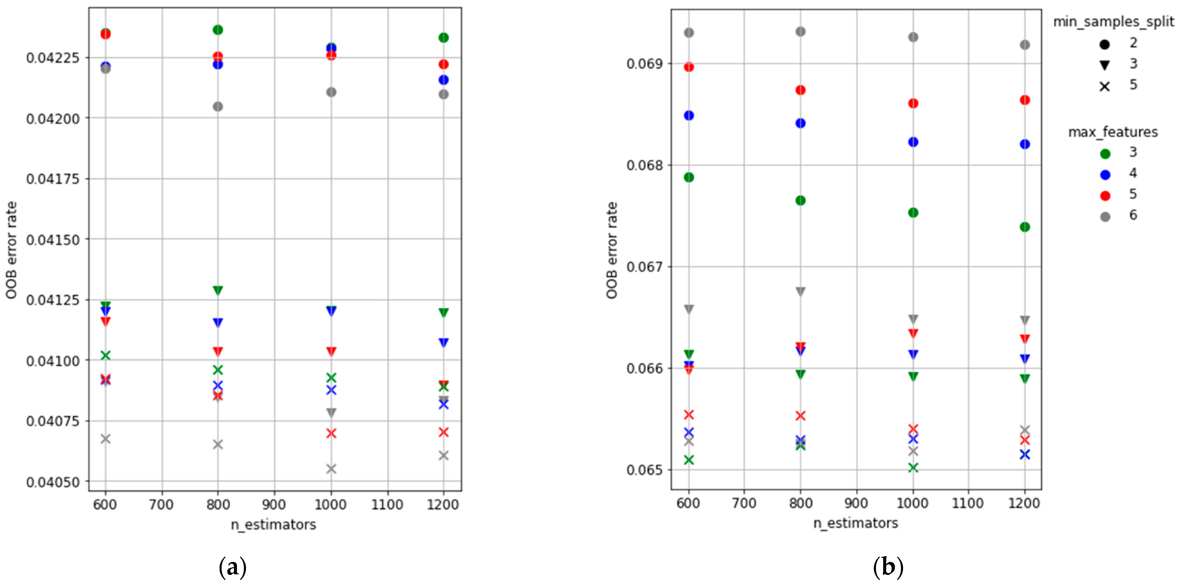
Figure 4 shows the OOB error score for all combinations of parameters tested for both the RF-OS and RF-US. Small variations of the OOB error are obtained among combinations, which confirm the previous findings regarding the robustness of the algorithm [52]. However, the combination corresponding to the lowest value was selected for both cases: n_estimators = 1000, min_sample_split = 5 and max_features = 6 for RF-OS and n_estimators = 1000, min_sample_split = 5 and max_features = 3 for RF-US.
Table 3 and Table 4 present the confusion matrix generated with the test set for each RF model, together with the accuracy metrics. RF-OS presented a larger recall score than RF-US, but the precision and accuracy scores are lower. Table 3 shows that the RF-OS model overestimated samples of Class 1 (many FP), affecting its overall performance. Conversely, the RF-US had good results for all scores, although recall is lower than RF-OS recall (more FN).
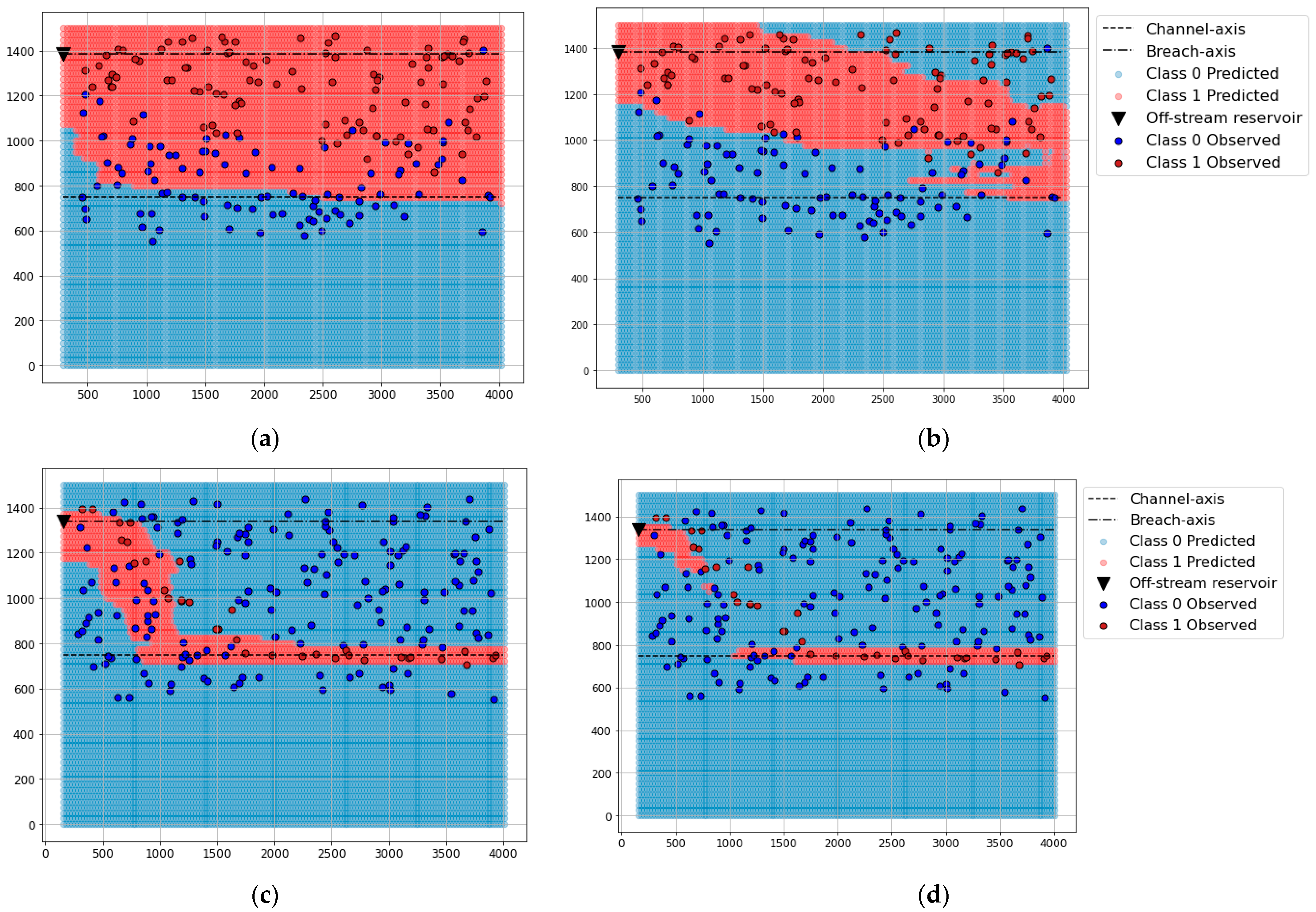
The differences in the performance between models were observed graphically for the cases in the test set (Supplementary material Section S1). As an example, Figure 5 presents maps of classification of potential hazard estimated with both models for two synthetic cases included in the test set corresponding to the larger (ID:084) and the smaller (ID:099) reservoir volume.
For high Manning coefficients, the maps generated with the RF-US model included most of the gauges of Class 1 estimated with Iber, although some class 0 gauges were incorrect. By contrast, the RF-OS estimated most of the area of the maps as Class 1, as observed in the confusion matrix. For lower Manning coefficients, RF-US provided better results.
These maps show only a few examples and might not represent the reality for all synthetic cases. Therefore, the analysis of the confusion matrix and precision metrics are more important than the graphic analysis. Consequently, the RF-US model was selected to carry out the study.
3.3. Analysis and Validation
3.3.1. Feature Importance
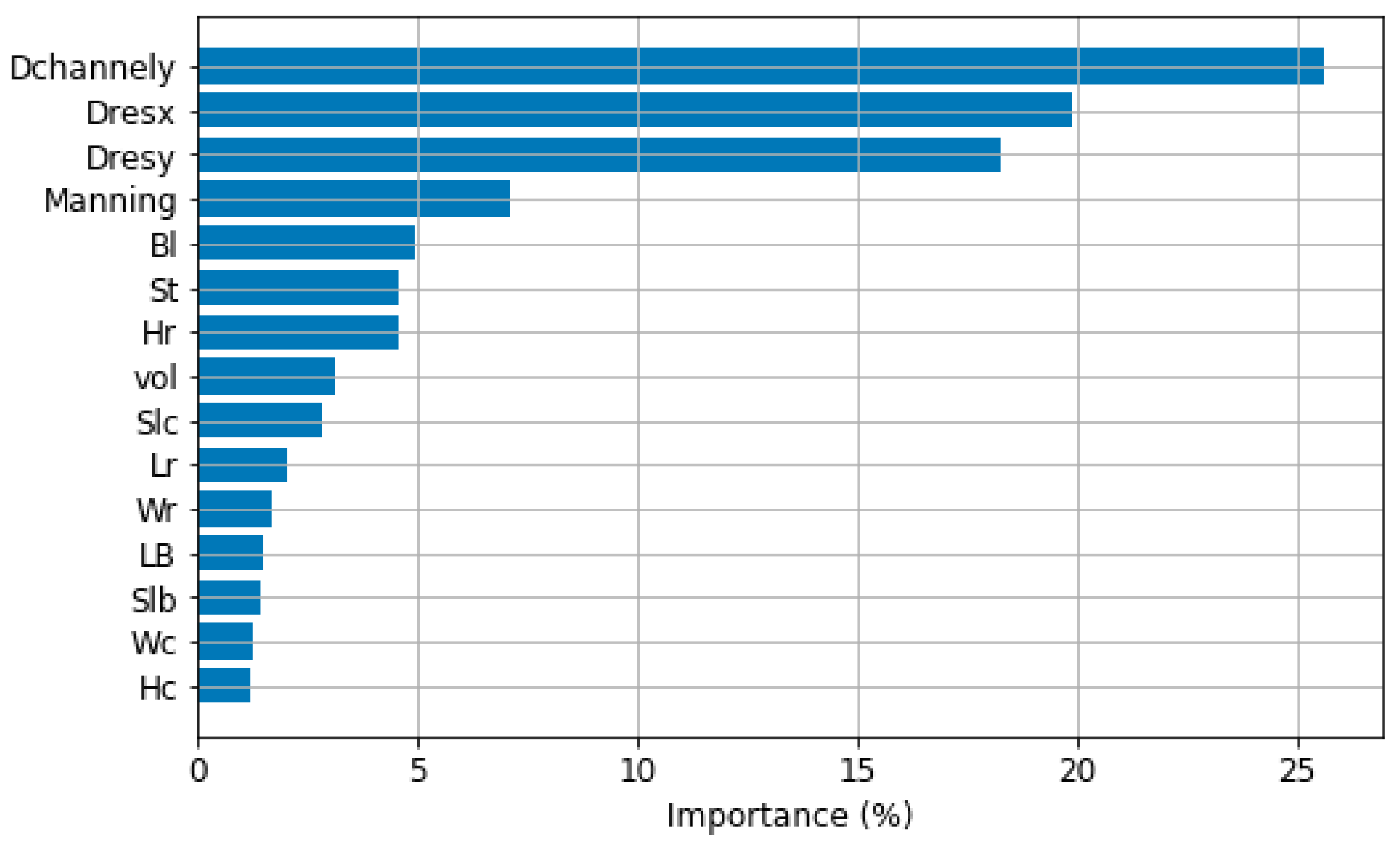
Feature importance provides an estimate of the influence of each input variable on the predictions of the RF model. Each feature is rated with a number between 0 and 1, computed by aggregating the feature importance over the trees in the model. The higher the number, the more important the variable [53].
Figure 6 presents the importance of each feature in the RF-US model. Those associated with the location of the gauges (Dchannely, Dresx and Dresy) have the highest importance, while the channel geometry (Wc and Hc) results have low relevance.
The performance of the chosen RF model (RF-US) was further analysed by means of the confusion matrix for the validation set (Table 5). The measures of accuracy were similar to those obtained for the test set.
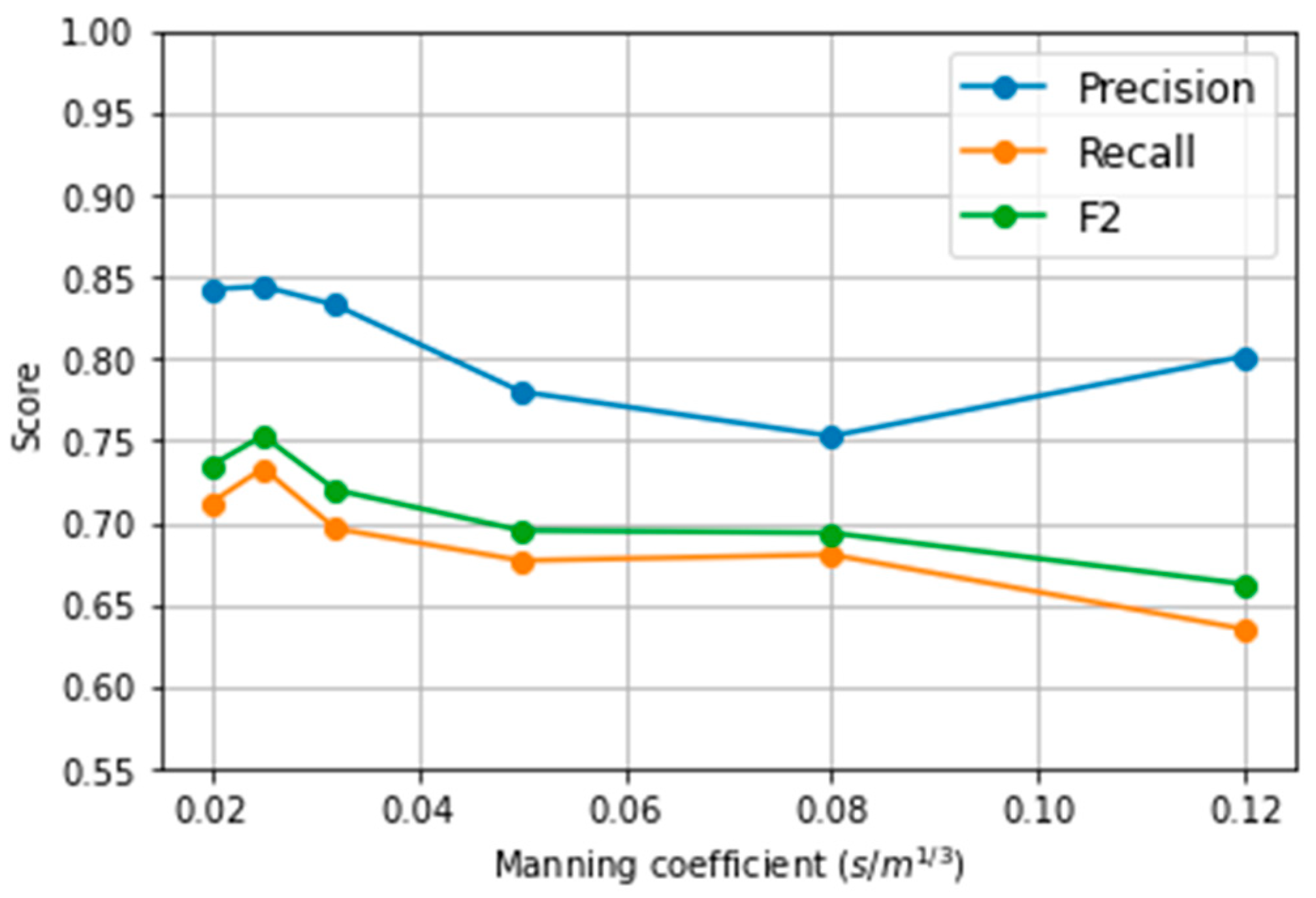
3.3.2. Effect of the Manning Coefficient
Since the Manning coefficient has the greatest influence on potential hazard after the gauge location (Figure 6), it was analysed in more detail. Figure 7 shows the results of precision, recall and F2 scores segregated by the Manning coefficient.
The F2 score tends to decrease as the Manning coefficient increases, probably because of the reduced size of the training set after undersampling for high Manning values (Figure 3).
3.3.3. Class Probability
RF models employ class probabilities to estimate the correct predicted class in each tree and in the overall prediction [54]. The classifier generates a positive or negative prediction based on a probability threshold, which equals 0.5 by default [46]. Predictions with high probabilities are expected to be more reliable than those close to 0.5. For example, two cases with probability of Class 1 equal to 0.51 and 0.99 will be taken as positives, but the prediction is more reliable for the latter. In this section, we analyse the probability threshold for the estimation of the classifier.
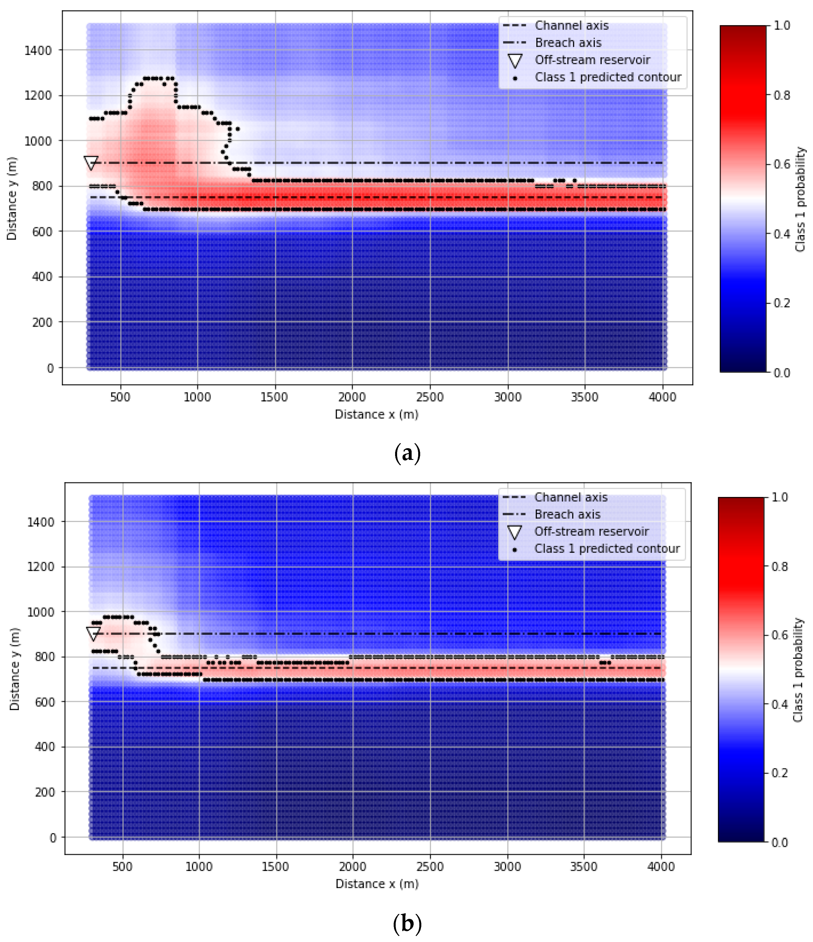
Probability maps of Class 1 were generated for each case of the validation set (Supplementary material Section S2). An example from the validation set with different Manning coefficients (0.02 m/s1/3 and 0.12 m/s1/3) is included in Figure 8, which corresponds to the larger reservoir volume (ID 001V). The maps show the probability for Class 1 estimated for the RF model, and the contour of the area identified as Class 1 (probability above 0.5).
The area classified as Class 1 in Figure 8b presents mainly probabilities near 0.5, while higher values are obtained for the smaller Manning (Figure 9a). This suggests that the model is less reliable for higher Manning coefficients.
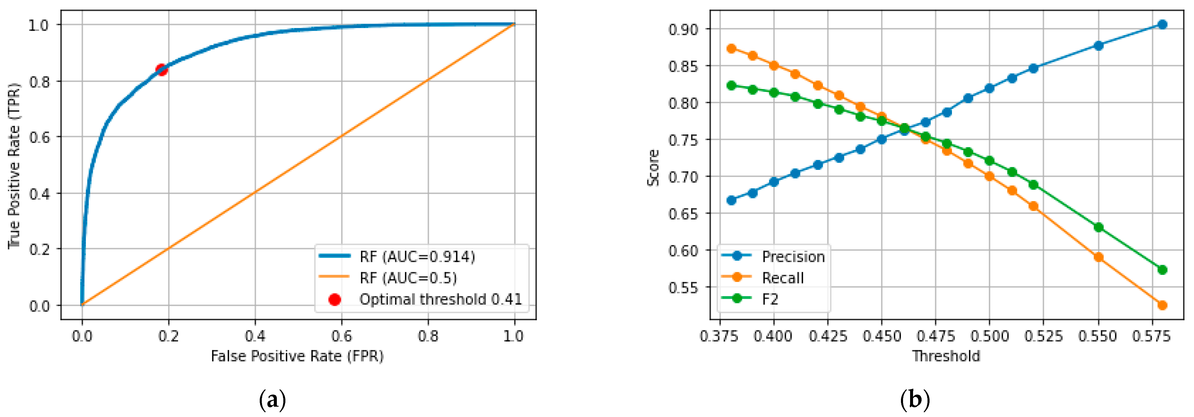
Figure 9a shows the ROC curve for the RF-US model estimated with the validation set and the corresponding AUC higher than 0.9. From the ROC curve, the optimal decision threshold was calculated (0.41), i.e., the value that ensures the best trade-off between the cost of failing to estimate TP against the cost of overestimating the positive class (FP).
The measures of accuracy were calculated for different decision thresholds, and they are plotted in Figure 9b. Decreasing the operating point ensures the estimation of more TP values; therefore, the recall and F2 scores increase. However, FP values increase as well, and the precision decreases.
Figure 10 shows the results for the optimal threshold as a function of Manning coefficient. Although the recall is higher than 0.8 for all coefficients, the precision is lower than for the default value (Class 1 overestimation).
4. Application to Real Case
4.1. Generation of Input Data
The application of the simplified model to a real case requires computing the input data for the ML model from the actual geometry of the reservoir (Wc, Wr, Lr, Hr, vol, Hc), the surrounding area (Bl, Slb, St, Slc, LB, Manning) and the location of vulnerable points (Dresx, Dresy and Dchannely), hereinafter the areas of interest (AoI). The geometrical parameters of the off-stream reservoir can be derived from the actual structure. By contrast, the remaining inputs must be converted from the real terrain to the parametrized geometry used for fitting the RF model.
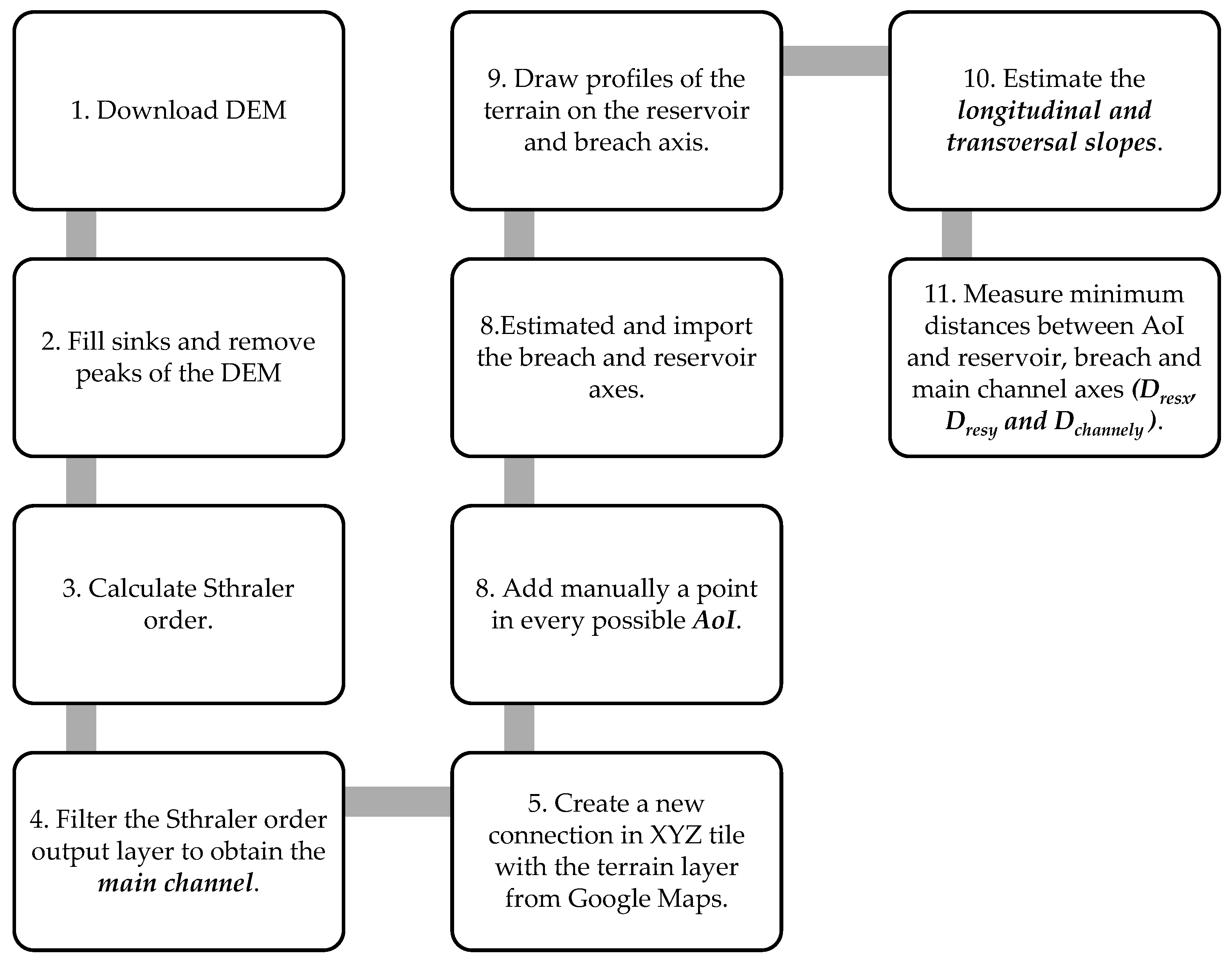
The Supplementary Material Section S3 includes a detailed guide for the parametrization of the real case using the open-access software QGIS [55]. Figure 11 shows an overview of the main tools for identification of the drainage network, selection of AoI and estimation of Dresx, Dresy and Dchannely for each AoI.
4.2. El Rubial Off-Stream Reservoir
The case of El Rubial off-stream reservoir, located in Alicante, Spain, was chosen to apply and validate the ML model. The reference solution was computed with the complete method (2D model on Iber) [56]. Three possible locations of the breach were considered: south dike (southeast corner), side dike (southwest corner) and north dike.
The DEM for the 2D model had a 5 m resolution, and the peak discharge and time of formation of the breach were calculated with the formulas and methods from Sanchez [57]. The physical characteristics of the off-stream reservoir and terrain are depicted in Table 6.
4.2.1. Main Channel and AoI
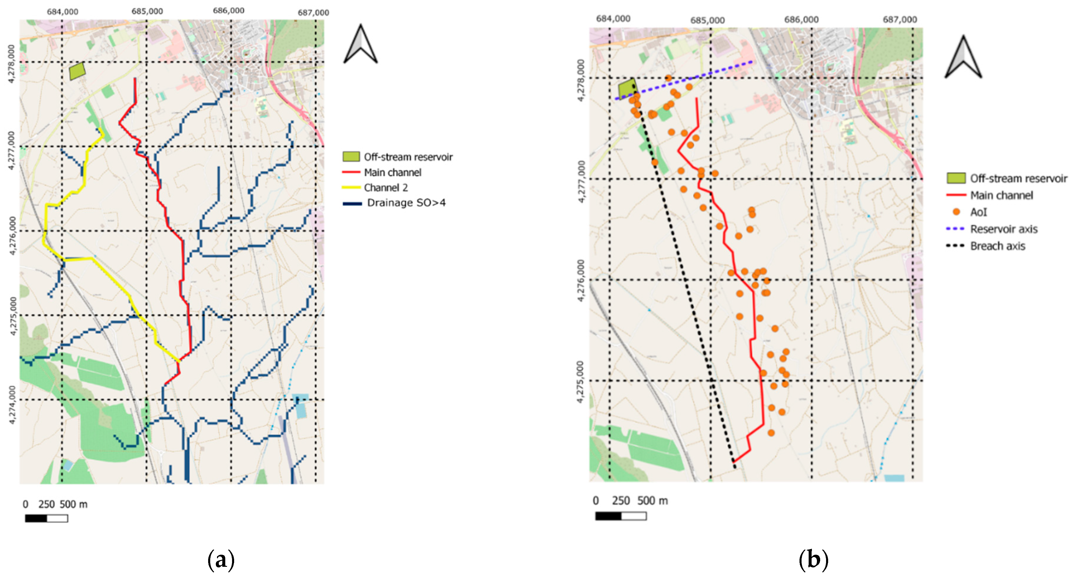
Figure 12a contains the drainage network of the area of study, obtained following the methodology explained in Supplementary Material Section S3. Pixels classified with a Strahler order higher than four were extracted. Although two paths can be identified downstream of the reservoir (red and yellow lines), only the main channel used in the reference document was considered. Nevertheless, the ML model can be applied for the two paths in real cases without information on the complete method.
The 56 AoI that may condition the category of the reservoir include houses, medium- and high-voltage poles and agricultural constructions. Their location is shown in Figure 12b together with the main channel and the reservoir and breach axes.
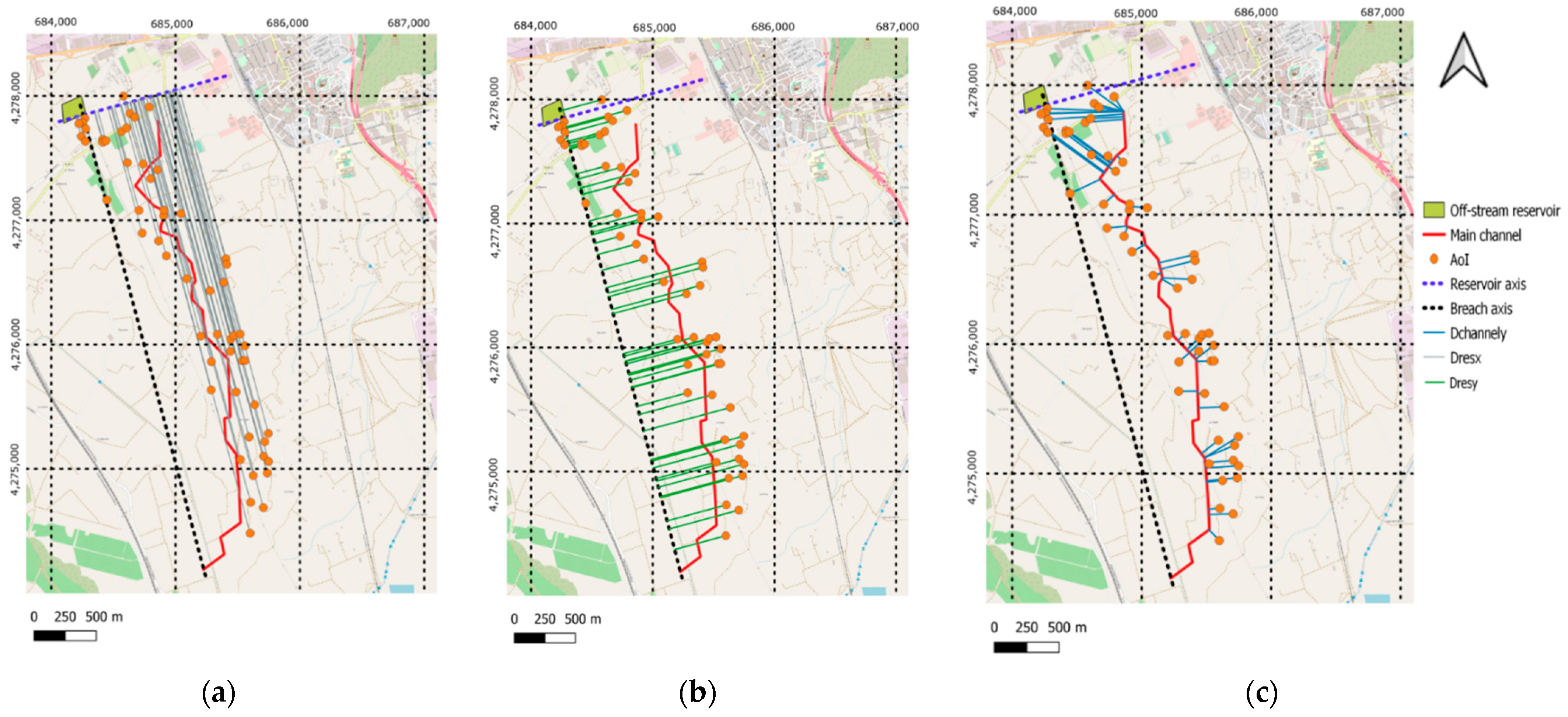
Following the procedure described in Supplementary Material Section S3, the breach and reservoir axes were estimated (rotation angle (θ) equal to 75°), and the minimum distances between the AoI and the three axes (Dresx, Dresy and Dchannely) were computed (Figure 13).
4.2.2. Terrain Parameters and Data Preparation
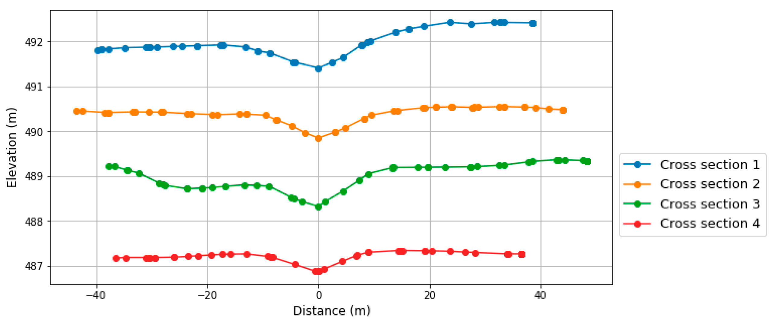
Figure 14 shows the cross sections at four locations extracted from the DEM used in Iber. Despite no main channel in the terrain, a “V” shape with around 10 m of width and 0.5 m of depth can be seen in the cross sections.
Additionally, the distance between the off-stream reservoir and the channel (Bl) was measured from the location of the main channel and the reservoir. Table 7 shows the estimated terrain parameters. A database with the 15 inputs for each AoI (Bl, Slb, Slc, St, LB, Wr, Lr, Hr, Hc, Wc, Manning, volume, Dchannel, Dresx and Dresy) was generated to apply the ML model.
4.3. Hazard Estimation Using the ML Model
4.3.1. Classification of Hazard with the Complete Method
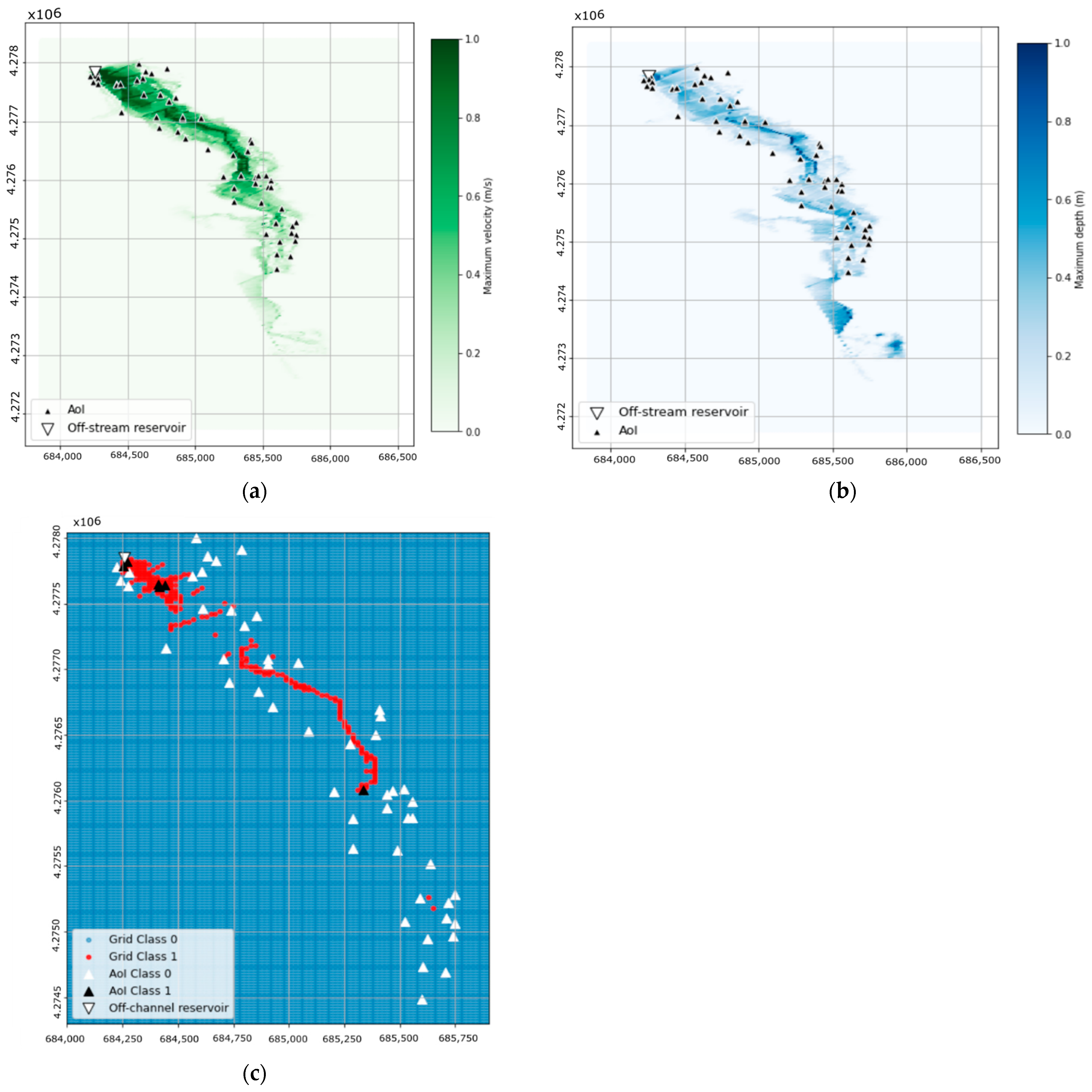
The maximum flow velocity and depth were extracted from the Iber model and were plotted over a 10 m × 10 m grid (Figure 15a,b). Figure 15c shows the potential hazard obtained from those results according to the Spanish regulation [1].
The same process was applied to the locations of the AoI, six of which resulted in Class 1 hazard (Figure 15c). This classification was taken as the reference to assess the ML model prediction.
4.3.2. Potential Hazard with the ML Model
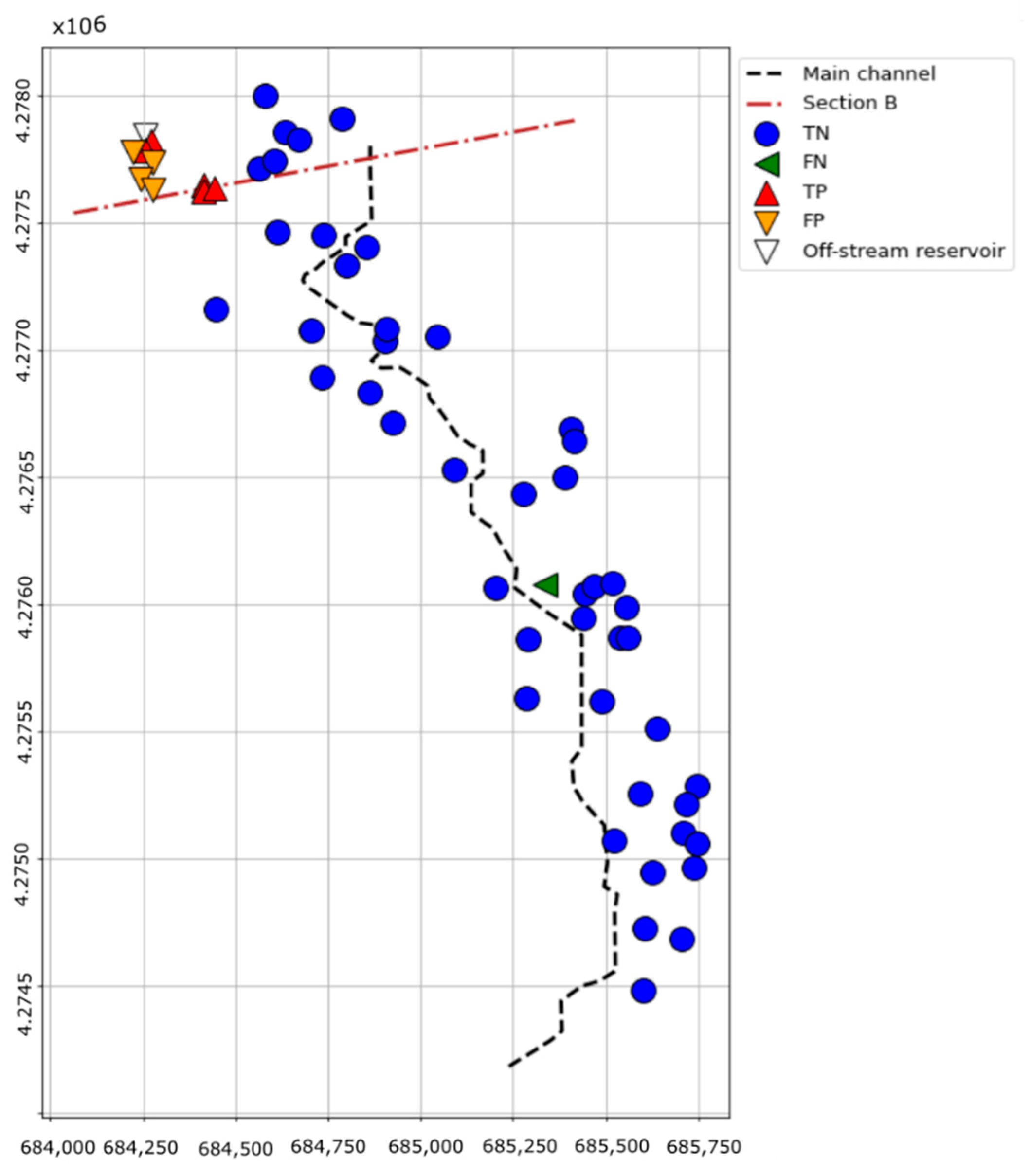
Table 8 shows the confusion matrix of the potential hazard for the 56 AoI. The results for all metrics considered are similar to those reported for the test set except for precision, i.e., the model overestimated the number of positives. The model correctly predicted 91% of the AoI.
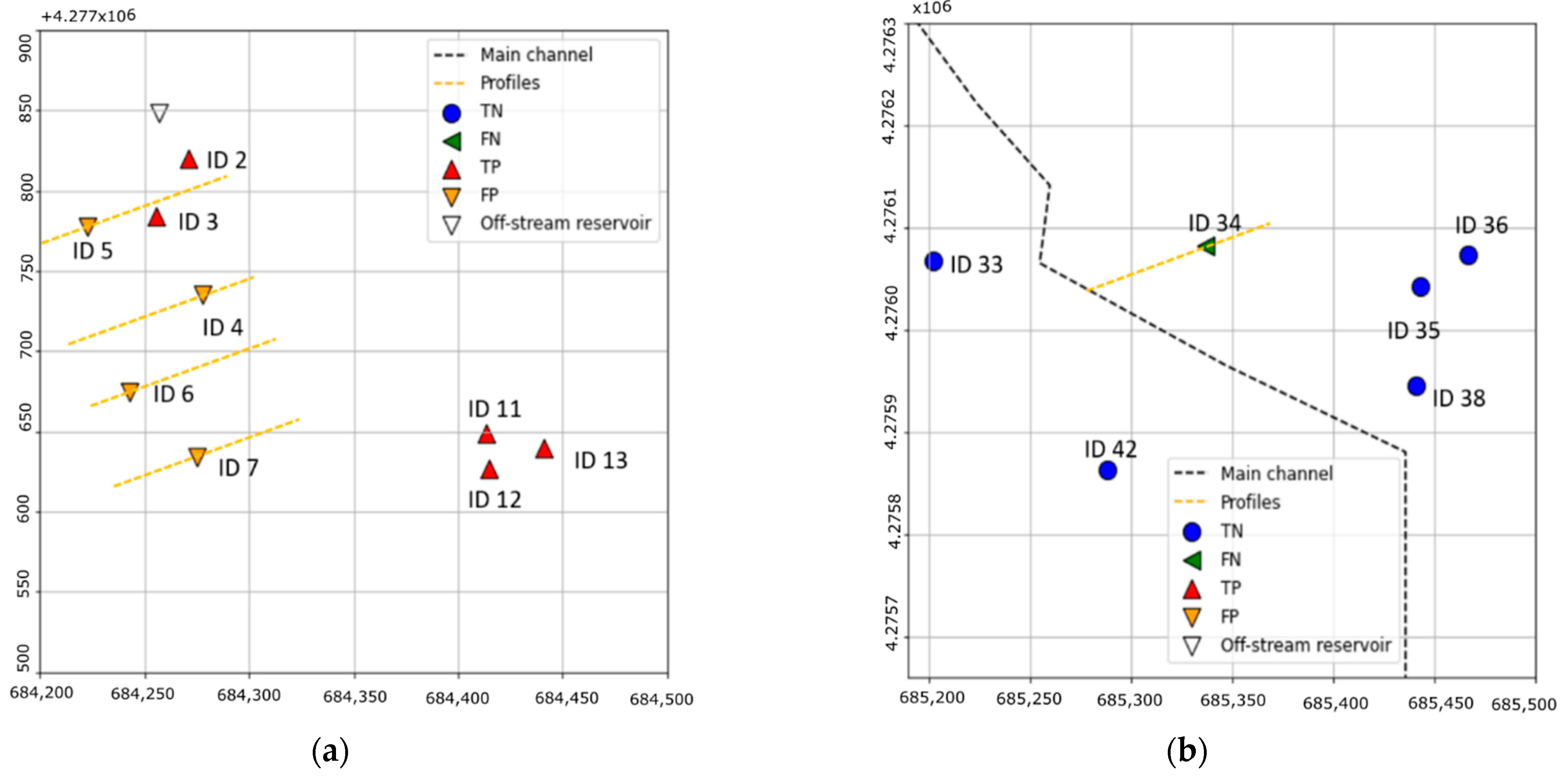
Figure 16 shows the predictions of the ML model. Five of the AoI near the off-stream reservoir are correctly identified (TP), and four AoI are misclassified (FP; Figure 17a). The observed AoI classified as Class 1 located most south was not correctly predicted by the ML model (FN; Figure 17b).
The misclassified AoI (FP and FN) were further examined. All FP are located in Section B in the simplified geometry, where the transversal slope is assumed to be null. However, the cross sections extracted from the DEM used in the Iber model (Figure 18) show that the AoI are located at higher elevations than the surrounding terrain, which means that the actual transversal slope is not zero. This could be the cause of the misclassification of the ML model.
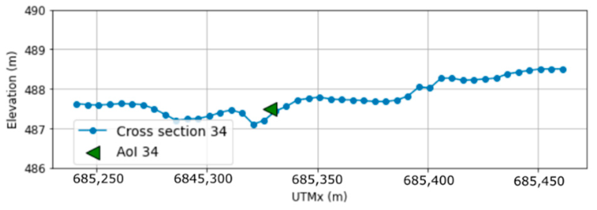
Figure 19 shows the terrain profile on the FN (ID 34). The AoI is located on the bank of the main channel, which means that the water depth is likely to be high. However, it is far from the main channel in the simplified geometry (Figure 17b), which is the probable source of the misclassification by the ML model.
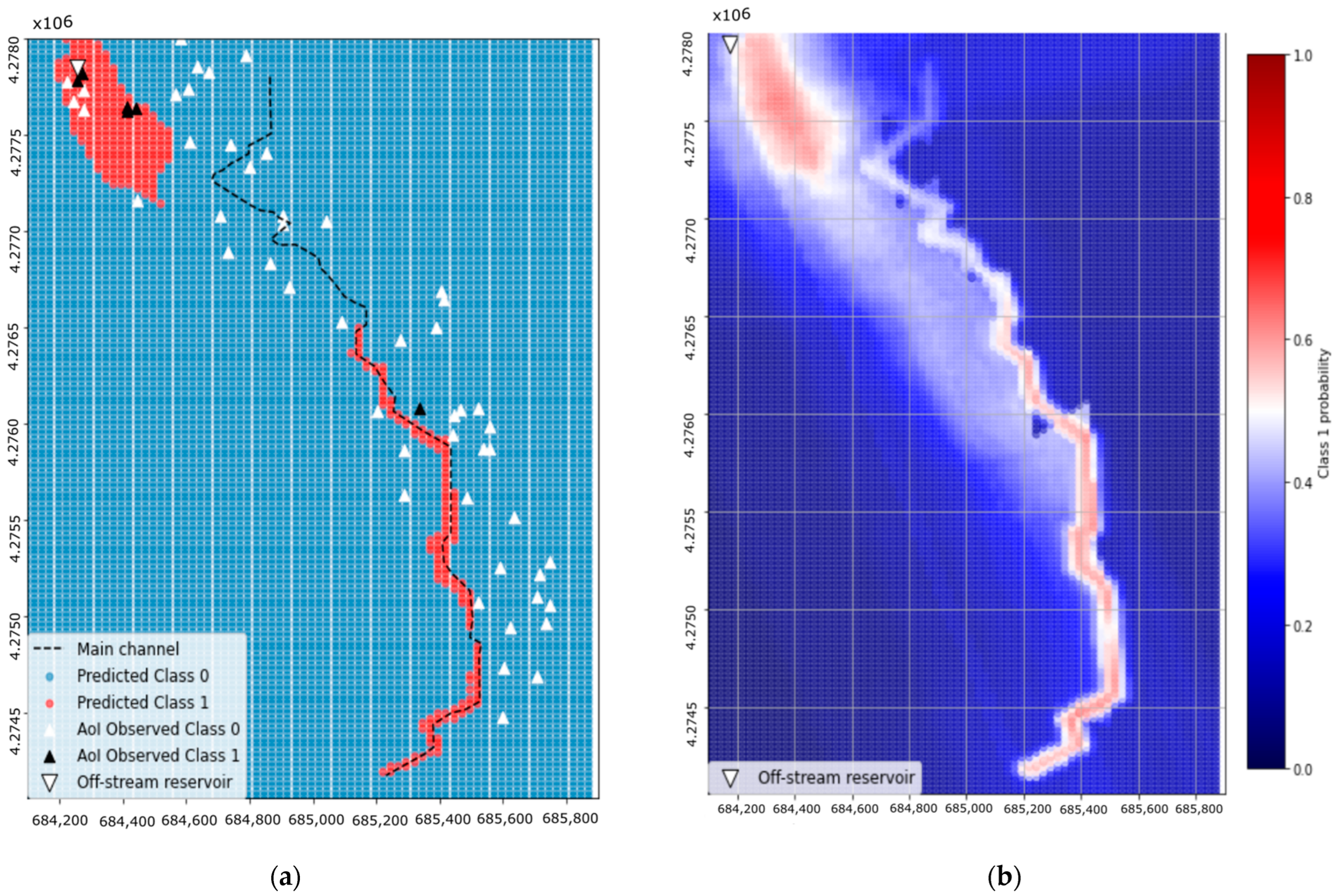
Figure 20a shows the predicted classification of potential hazard for the complete area of study. The Class 1 areas observed with the complete method (Figure 15c) and those predicted with the ML model present similar patterns, with a broad area considered as Class 1 near the reservoir. However, the ML model predicted most of the main channel as Class 1.
Figure 20b shows the results of the ML model as probability of Class 1. Most of the area predicted as Class 1 in the vicinity of the reservoir shows probabilities between 0.5 and 0.6, i.e., with high uncertainty. Higher values (more reliable predictions) are recorded in the main channel.
5. Discussion
Automating the generation of geometries and the execution of calculations in Iber obtained a useful database for training ML models. The developed process offers possibilities for the application of Iber in other types of analyses in which cases need to be systematically executed, such as probabilistic studies or sensitivity analyses [58,59,60,61]. Similar processes are already in application to generate training sets for ML surrogate models in hydrological studies [62,63,64], as well as to analyse the effect of breach properties on the floodplain [65,66].
The calibration of the RF models was performed by means of grid search over the parameters to choose, and the best combination was selected based on the OOB error. The results showed small variation in the OOB error among combinations, which confirms previous findings regarding the robustness of the algorithm [52]. The interpretation of the model in terms of the variable importance agrees with engineering intuition since the location of the AoI relative to the reservoir and the main channel were identified as the most relevant.
By contrast, the class distribution in the training set showed a clear effect on the performance of the models. RF-OS was trained with approximately 120,000 Class 1 samples, while the RF-US dataset had around 50,000 samples. The large training set for RF-OS produced an overestimation of Class 1, which led to lower accuracy and precision scores. Both methods can be further tuned to obtain more accurate models in general and in particular, to improve some of the accuracy indexes. For example, our results already showed that SMOTE is better for recall and worst for precision. However, the overall performance for practical applications is more dependent on other aspects, as described later.
In addition, the effect of the class distribution was associated with the Manning coefficient. For a given reservoir and domain, higher values of Manning result in low velocity and risk and thus in more points belonging to Class 0 (Figure 3). This also implies that the majority of samples in RF-OS are artificial, i.e., generated by k-nearest neighbours. Consequently, high amount of FP is reported for RF-OS. Additionally, the probability class analysis showed lower confidence of predictions (probabilities close to 0.5) in cases with larger Manning coefficients (Figure 8). The results in terms of class probability provide additional information that can be considered for decision making. In this regard, other algorithms more specifically developed for considering uncertainty may also be useful, such as deep Gaussian processes [67,68].
The use of regression ML models could be considered as an alternative to the proposed procedure, i.e., models to predict the numerical value of water depth and velocity. The drawback of this approach is that it would be necessary to use two models in parallel for both variables involved in the risk estimation. In addition, the problem of imbalanced training set remains, as there would be a much higher number of points with low (Class 0) versus high (Class 1) velocity and depth. Although there are procedures to balance training sets for regression, the process should be performed twice for both variables.
The results of Iber models have been considered as the reference solution (“ground truth” in machine learning terminology) throughout this work. This allowed for analysing the prediction capacity of the algorithm itself and the effect of aspects such as the training parameters and the balance of the sample or the threshold. The models used for the validation set follow the same scheme as those in the training set, defined in Figure 1. This is reflected in the similarity between the results obtained for the test set (Table 4) and the validation set (Table 5) for all the indices considered.
On the contrary, the case of the El Rubial reservoir presents relevant differences with respect to the artificial geometries. First, the parameterization of the geometry implies a relevant simplification of the real terrain: a constant cross-section of the main channel is used, the roughness is unique for the entire model, and average values are taken for longitudinal and transverse slopes of sections B and C. This implies a loss of accuracy. However, the results regarding the classification suggest that the main cause of the discrepancy is the resolution of the DEM used, which is higher in the complete (5 m) than in the simplified model (30 m). This is clearly the origin of the observed FN (Figure 19) and is related to the FN recorded in the vicinity of the reservoir.
The definition of section B, where all FP are located, is also influential in prediction accuracy. While no transversal slope is considered in this section in the parameterized geometry, the profiles from the high-resolution DEM (Figure 18) show a slope towards the northeast that conveys the main flow towards that area in the complete model, away from the AoI, which remains unaffected. This is not considered in the simplified model, which results in a large area classified as Class 1 in the vicinity of the reservoir (Figure 20).
Although the developed model is based on the risk criteria defined by Spanish regulations, the methodology can be directly applied to other criteria, such as those proposed by Smith et al. [69]. The models from the training database could be used with the only change of adapting the class of each point to the criteria used based on the water velocity and depth. It would suffice to train a new model with the adjusted classification, which has a low computational cost.
A limitation of the methodology and the simplified model is due to the dimensions of the domain considered and, in general, to the ranges of variation used to define the parameters of the models in the training set (Table 1). Although they have been selected to represent the most common geometry of this type of reservoirs and its surrounding terrain, there may be cases with dimensions outside these ranges, either for the reservoir or the terrain (dimensions of the main channel or slopes). It is well known that ML-based models are unreliable when applied to cases outside the range of variation of the training data. This can be solved by expanding the training database with more cases with wider ranges of variation. As mentioned before, the cases already calculated can be used to train new, more accurate ML models.
The application of the ML model to a real case led to the development of a step-by-step procedure based on the open-source software QGIS (Figure 11). Although the definition of the parameters of the simplified geometry and the location of the AoI involve several steps involving GIS tools, the process is simpler and faster to implement than the complete method. In addition, the necessary information can also be obtained from free online tools, with lower requirements in terms of time and software.
Despite the described limitations of the model and the differences with the actual El Rubial reservoir, the ML model correctly predicted 91% of the AoI. This accuracy is higher than that obtained in related studies [12,13], although they cannot be directly compared due to the existing differences. Correct identification of parameters and selection of DEM is critical for the performance of the model: DEM with a small resolution can result in a more detailed drainage network and a better selection of the main channel.
6. Summary and Conclusions
A simplified methodology is presented to estimate the zones with risk to human life in case of a failure of an off-stream reservoir, based on the Spanish regulations (Class 0: no risk, Class 1: risk). The methodology makes use of a surrogate ML model based on RF and trained with a set of artificial cases automatically generated and run with Iber. Given the results for maximum flow velocity and depth, points are classified as a function of the risk to human life. The inputs to the ML model include geometrical parameters of the reservoir and surrounding area and the location of the AoI concerning the reservoir and the main channel.
The imbalanced distribution of classes in the training had a great effect in the performance of the surrogate models. Two approaches were assessed to alleviate this issue: SMOTE and random undersampling. Although the accuracy and OOB error rate of both RF models were similar, the use of different balanced datasets affects the model’s capacity to predict the risk zones. The RF-US model presented measures of accuracy higher than 0.8 and a superior capacity to estimate Class 1 areas. The model was assessed with a validation dataset, analysing the influences of the Manning coefficient, class probability and operating point of the RF model.
The analysis of the ROC curve and variation of the operating point to estimate risk areas showed that lowering the decision threshold could enhance the F2 score, especially in cases with larger roughness. However, this leads to an overestimation of risk areas. The selection of the operating point depends on the nature of the case and the preferences of the modeller.
The application of the ML model to a real case showed the needed efforts to extract the input data. The identification of the main flow path and location of AoI are essential for accurate predictions. The results are highly dependent on the quality of the geometrical information provided: the resolution of the DEM and the similarities between the simplified and the actual geometry. The best choice should be a trade-off between desired accuracy and available resources. Nonetheless, the simplified methodology can be applied in any setting and requires less time and computational resources. Therefore, the simplified RF model can be useful for owners and administrations of off-stream reservoirs to prioritize the allocation of resources to carry out detailed classification studies or to make investments to increase safety.
Supplementary Materials
The following supporting information can be downloaded at: https://www.mdpi.com/article/10.3390/w14152416/s1, Section S1: Figure S1: Maps of classification of risk with RF-OS and RF-US for the test set; every figure is named with the RF model, its ID and land use, Table S1: Parameters test set. Section S2: Figure S2: Maps of the probability of Class 1 with RF-US for the validation set; every figure is named with its ID and land use, Table S2: Parameters validation set. Section S3: Guide for computing the input data for the ML model using QGIS. Refs [55,70,71,72,73,74,75,76,77] are cited in Supplementary Materials.
Author Contributions
Conceptualization, N.S.-C., F.S., M.S.-R. and E.B.; methodology, N.S.-C., M.S.-R., F.S. and E.B.; validation, N.S.-C.; formal analysis, N.S.-C.; data curation, N.S.-C.; writing—original draft preparation, N.S.-C. and F.S.; writing—review and editing, N.S.-C., F.S., M.S.-R. and E.B.; funding acquisition, F.S. and E.B. All authors have read and agreed to the published version of the manuscript.
Funding
This work was partially funded by the Spanish Ministry of Science, Innovation and Universities through the Projects ACROPOLIS (RTC2019-007343-5), TRISTAN (RTI2018-094785-B-I00) and DOLMEN (PID2021-122661OB-I00), as well as by the Spanish Ministry of Economy and Competitiveness, through the “Severo Ochoa Programme for Centres of Excellence in R & D” (CEX2018-000797-S), and by the Generalitat de Catalunya through the CERCA Program.
Institutional Review Board Statement
Not applicable.
Informed Consent Statement
Not applicable.
Data Availability Statement
The data presented in this study are available on request from the corresponding author.
Acknowledgments
The authors thank “Junta Central de Usuarios del Vinalopó, L’ Alacantí y Consorcio de Aguas de la Marina Baja” (JCU) for interest in the ACROPOLIS Project, as well as his collaboration and generous work of information searching. Additional thanks to “Comunidad de Regantes de Huerta y Partidas de Villena” and ARVUM, who provided us the information of ‘El Rubial’ study case. Finally, thanks to V.J. Richart, a technician from JCU, for his interest in the project and developments.
Conflicts of Interest
The authors declare no conflict of interest.
References
- Ministry of the Presidency. Real Decreto 9/2008, de 11 de enero, por el que se Modifica el Reglamento del Dominio Público Hidráulico, Aprobado por el Real Decreto 849/1986, de 11 de abril [Royal Decree 9/2008, of 11 January, Amending the Regulations on the Public Hydraulic Domain, Approved by Royal Decree 849/1986, of 11 April.] BOE Núm 2008, pp. 3141–3149. Available online: https://www.boe.es/buscar/doc.php?id=BOE-A-2008-755 (accessed on 26 June 2022).
- De Cea, C. Evolución de La Normativa En Seguridad de Balsas de Riego [Developments in Irrigation Pond Safety Regulations]. In Proceedings of the Conference on the Management of Safety in Irrigation Ponds, Online, 19 July 2021. [Google Scholar]
- Ministry for the Ecological Transition and the Demographic Challenge Guía Técnica Para la Clasificación de Presas [Technical Guide Dam Clasification] 2021. Available online: https://www.miteco.gob.es/es/agua/temas/seguridad-de-presas-y-embalses/guiatecnicaclasificacion_adaptacionants_nov2021_v16_tcm30-533050.pdf (accessed on 26 June 2022).
- MMA. Technical Guide for Dam Classification Funtion of the Potential Risk; Ministerio de Medio Ambiente (MMA), Dirección General de Obras Hidráulicas y Calidad de las Aguas: Madrid, Spain, 1996; p. 63. [Google Scholar]
- Fread, D.L. The NWS DAMBRK Model: Theoretical Background/User Documentation; Hydrologic Research Laboratory, National Weather Service, NOAA: Washington, DC, USA, 1988.
- Wetmore, J.N.; Fread, D.L. The NWS Simplified Dam-Break Flood Forecasting Model; National Weather Service: Silver Spring, MD, USA, 1981; pp. 164–197.
- Bladé Castellet, E.; Cea, L.; Corestein, G.; Escolano, E.; Puertas, J.; Vázquez-Cendón, E.; Dolz, J.; Coll, A. Iber: Herramienta de simulación numérica del flujo en ríos [Iber: Tool for numerical simulation of river flow]. Rev. Int. Métod. Numér. Para Cálculo Diseño Ing. 2014, 30, 1–10. [Google Scholar] [CrossRef] [Green Version]
- Soler, J.; Bladé, E.; Sánchez-Juny, M. Comparasion of Unidimensional and Bidimensional Flow Models for Earthen Dam Failures. Rev. Int. Métod. Numér. Para Cálculo Diseño En Ing. 2012, 28, 103–111. [Google Scholar] [CrossRef] [Green Version]
- Espejo Almodóvar, F.A. Caracterización del Funcionamiento y Control Hidráulico Frente a la Rotura de Balsas de Riego, Mediante un Marco de Trabajo Estocástico [Characterization of the Operation and Hydraulic Control against the Breakage of Irrigation Ponds, through a Stochastic Framework]. Ph.D. Thesis, Salamanca University, Salamanca, Spain, 2017. [Google Scholar]
- Hori, T.; Izumi, A.; Shoda, D.; Shigeoka, T.; Yoshisako, H. Development of Disaster Prevention Support System for Irrigation Pond (DPSIP). J. Disaster. Res. 2019, 14, 303–314. [Google Scholar] [CrossRef]
- Sánchez-Romero, F.J.; Pérez-Sánchez, M.; Redón-Santafé, M.; Torregrosa Soler, J.B.; Ferrer Gisbert, C.; Ferrán Gozálvez, J.J.; Ferrer Gisbert, A.; López-Jiménez, P.A. Estudio numérico para la elaboración de mapas de inundación considerando la hipótesis de rotura en balsas para riego [Numerical study for the elaboration of flood maps considering the hypothesis of breaching in irrigation ponds]. Ing. Agua 2019, 23, 1. [Google Scholar] [CrossRef]
- Cannata, M.; Marzocchi, R. Two-Dimensional Dam Break Flooding Simulation: A GIS-Embedded Approach. Nat. Hazards 2012, 61, 1143–1159. [Google Scholar] [CrossRef]
- Albano, R.; Mancusi, L.; Adamowski, J.; Cantisani, A.; Sole, A. A GIS Tool for Mapping Dam-Break Flood Hazards in Italy. Int. J. Geo-Inf. 2019, 8, 250. [Google Scholar] [CrossRef] [Green Version]
- Hooshyaripor, F.; Tahershamsi, A.; Behzadian, K. Estimation of Peak Outflow in Dam Failure Using Neural Network Approach under Uncertainty Analysis. Water Resour. 2015, 42, 723–736. [Google Scholar] [CrossRef] [Green Version]
- Hooshyaripor, F.; Tahershamsi, A.; Golian, S. Application of Copula Method and Neural Networks for Predicting Peak Outflow from Breached Embankments. J. Hydro-Environ. Res. 2014, 8, 292–303. [Google Scholar] [CrossRef]
- Salazar, F.; Toledo, M.; Oñate, E.; Morán, R. An Empirical Comparison of Machine Learning Techniques for Dam Behaviour Modelling. Struct. Saf. 2015, 56, 9–17. [Google Scholar] [CrossRef] [Green Version]
- Mata, J.; Salazar, F.; Barateiro, J.; Antunes, A. Validation of Machine Learning Models for Structural Dam Behaviour Interpretation and Prediction. Water 2021, 13, 2717. [Google Scholar] [CrossRef]
- Fisher, W.D.; Camp, T.K.; Krzhizhanovskaya, V.V. Anomaly Detection in Earth Dam and Levee Passive Seismic Data Using Support Vector Machines and Automatic Feature Selection. J. Comput. Sci. 2017, 20, 143–153. [Google Scholar] [CrossRef]
- Salazar, F.; Conde, A.; Irazábal, J.; Vicente, D.J. Anomaly Detection in Dam Behaviour with Machine Learning Classification Models. Water 2021, 13, 2387. [Google Scholar] [CrossRef]
- Hariri-Ardebili, M.A.; Pourkamali-Anaraki, F. Simplified Reliability Analysis of Multi Hazard Risk in Gravity Dams via Machine Learning Techniques. Arch. Civ. Mech. Engl. 2018, 18, 592–610. [Google Scholar] [CrossRef]
- Sachdeva, S.; Bhatia, T.; Verma, A.K. Flood Susceptibility Mapping Using GIS-Based Support Vector Machine and Particle Swarm Optimization: A Case Study in Uttarakhand (India). In Proceedings of the 2017 8th International Conference on Computing, Communication and Networking Technologies (ICCCNT), Delhi, India, 3–7 July 2017; IEEE: Delhi, India, 2017; pp. 1–7. [Google Scholar]
- Motta, M.; de Castro Neto, M.; Sarmento, P. A Mixed Approach for Urban Flood Prediction Using Machine Learning and GIS. Int. J. Disaster Risk Reduct. 2021, 56, 102154. [Google Scholar] [CrossRef]
- Bladé Castellet, E.; Cea, L.; Corestein, G. Numerical Modelling of River Inundations. Ing. Agua 2014, 18, 71–82. [Google Scholar] [CrossRef]
- Stein, M. Large Sample Properties of Simulations Using Latin Hypercube Sampling. Technometrics 1987, 29, 143–151. [Google Scholar] [CrossRef]
- Mckay, M.D.; Beckman, R.J.; Conover, W.J. A Comparison of Three Methods for Selecting Values of Input Variables in the Analysis of Output From a Computer Code. Technometrics 2000, 42, 55–61. [Google Scholar] [CrossRef]
- Cea, L.; Bladé, E. A Simple and Efficient Unstructured Finite Volume Scheme for Solving the Shallow Water Equations in Overland Flow Applications. Water Resour. Res. 2015, 51, 5464–5486. [Google Scholar] [CrossRef] [Green Version]
- Sanz-Ramos, M.; Bladé, E.; González-Escalona, F.; Olivares, G.; Aragón-Hernández, J.L. Interpreting the Manning Roughness Coefficient in Overland Flow Simulations with Coupled Hydrological-Hydraulic Distributed Models. Water 2021, 13, 3433. [Google Scholar] [CrossRef]
- Cea, L.; Bermúdez, M.; Puertas, J.; Bladé, E.; Corestein, G.; Escolano, E.; Conde, A.; Bockelmann-Evans, B.; Ahmadian, R. IberWQ: New Simulation Tool for 2D Water Quality Modelling in Rivers and Shallow Estuaries. J. Hydroinform. 2016, 18, 816–830. [Google Scholar] [CrossRef] [Green Version]
- Ruiz-Villanueva, V.; Bladé, E.; Sánchez-Juny, M.; Marti-Cardona, B.; Díez-Herrero, A.; Bodoque, J.M. Two-Dimensional Numerical Modeling of Wood Transport. J. Hydroinform. 2014, 16, 1077–1096. [Google Scholar] [CrossRef]
- Sanz-Ramos, M.; Bladé Castellet, E.; Palau Ibars, A.; Vericat Querol, D.; Ramos-Fuertes, A. IberHABITAT: Evaluación de La Idoneidad Del Hábitat Físico y Del Hábitat Potencial Útil Para Peces. Aplicación En El Río Eume [IberHABITAT: Assessment of Physical Habitat Suitability and Weighted Usable Area for Fishes. Application in the Eume River]. Ribagua 2019, 6, 158–167. [Google Scholar] [CrossRef] [Green Version]
- Coll, A.; Escolano, E.; Pasenau, M.; Monros, A. GiD for Science. GiD Simulation [WWW Document]. 2022. Available online: https://www.gidsimulation.com/gid-for-science/examples/ (accessed on 26 July 2022).
- Sanz-Ramos, M.; Olivares Cerpa, G.; Bladé i Castellet, E. Metodología Para El Análisis de Rotura de Presas Con Aterramiento Mediante Simulación Con Fondo Móvil [Methodology for Dam Failure Analysis with Grounding Using Moving Bottom Simulation]. Ribagua 2019, 6, 138–147. [Google Scholar] [CrossRef] [Green Version]
- Álvarez, M.; Puertas, J.; Peña, E.; Bermúdez, M. Two-Dimensional Dam-Break Flood Analysis in Data-Scarce Regions: The Case Study of Chipembe Dam, Mozambique. Water 2017, 9, 432. [Google Scholar] [CrossRef] [Green Version]
- Coll, A.; Ribó, R.; Escolano, E.; Perez, J.; Melendo, A.; Monros, A.; Gárate, J. GiD v.14 User Manual. Available online: www.gidsimulation.com (accessed on 29 July 2022).
- García-Feal, O.; González-Cao, J.; Gómez-Gesteira, M.; Cea, L.; Domínguez, J.M.; Formella, A. An Accelerated Tool for Flood Modelling Based on Iber. Water 2018, 10, 1459. [Google Scholar] [CrossRef] [Green Version]
- Salazar, F.; Crookston, B.M. A Performance Comparison of Machine Learning Algorithms for Arced Labyrinth Spillways. Water 2019, 11, 544. [Google Scholar] [CrossRef] [Green Version]
- Ko, B.C.; Kim, H.H.; Nam, J.Y. Classification of Potential Water Bodies Using Landsat 8 OLI and a Combination of Two Boosted Random Forest Classifiers. Sensors 2015, 15, 13763–13777. [Google Scholar] [CrossRef] [PubMed] [Green Version]
- Feng, Q.; Liu, J.; Gong, J. Urban Flood Mapping Based on Unmanned Aerial Vehicle Remote Sensing and Random Forest Classifier—A Case of Yuyao, China. Water 2015, 7, 1437–1455. [Google Scholar] [CrossRef]
- Tyralis, H.; Papacharalampous, G.; Langousis, A. A Brief Review of Random Forests for Water Scientists and Practitioners and Their Recent History in Water Resources. Water 2019, 11, 910. [Google Scholar] [CrossRef] [Green Version]
- Breiman, L. Random Forests. Mach. Learn. 2001, 45, 5–32. [Google Scholar] [CrossRef] [Green Version]
- Najafzadeh, M.; Oliveto, G. Riprap Incipient Motion for Overtopping Flows with Machine Learning Models. J. Hydroinform. 2020, 22, 749–767. [Google Scholar] [CrossRef]
- Salazar, F.; Hariri-Ardebili, M.A. Coupling Machine Learning and Stochastic Finite Element to Evaluate Heterogeneous Concrete Infrastructure. Engl. Struct. 2022, 260, 114190. [Google Scholar] [CrossRef]
- Pedregosa, F.; Varoquaux, G.; Gramfort, A.; Michel, V.; Thirion, B.; Grisel, O.; Blondel, M.; Prettenhofer, P.; Weiss, R.; Dubourg, V.; et al. Scikit-Learn: Machine Learning in Python. J. Mach. Learn. Res. 2011, 12, 2825–2830. [Google Scholar]
- Batista, G.E.A.P.A.; Prati, R.C.; Monard, M.C. A Study of the Behavior of Several Methods for Balancing Machine Learning Training Data. ACM SIGKDD Explor. Newsl. 2004, 6, 21–29. [Google Scholar] [CrossRef]
- Chawla, N.V.; Bowyer, K.W.; Hall, L.O.; Kegelmeyer, W.P. SMOTE: Synthetic Minority Over-Sampling Technique. J. Artif. Intell. Res. 2002, 16, 321–357. [Google Scholar] [CrossRef]
- Fernández, A.; García, S.; Galar, M.; Prati, R.C.; Krawczyk, B.; Herrera, F. Learning from Imbalanced Datasets; Springer: Berlin/Heidelberg, Germany, 2018; ISBN 978-3-319-98074-4. [Google Scholar]
- Zhang, C.; Ma, Y. Ensemble Machine Learning: Methods and Applications; Springer: New York, NY, USA, 2012; ISBN 978-1-4419-9326-7. [Google Scholar]
- Hastie, T.; Tibshirani, R.; Friedman, J. The Elements of Statistical Learning: Data Mining, Inference, and Prediction, 2nd ed.; Springer: New York, NY, USA, 2017; ISBN 978-0-387-84857-0. [Google Scholar]
- Farhadi, H.; Najafzadeh, M. Flood Risk Mapping by Remote Sensing Data and Random Forest Technique. Water 2021, 13, 3115. [Google Scholar] [CrossRef]
- Chen, Y.-W.; Lin, C.-J. Combining SVMs with Various Feature Selection Strategies. In Studies in Fuzziness and Soft Computin; Springer: Berlin/Heidelberg, Germany, 2006; Volume 207, pp. 315–324. [Google Scholar] [CrossRef] [Green Version]
- Huang, J.; Ling, C.X. Using AUC and Accuracy in Evaluating Learning Algorithms. IEEE Trans. Knowl. Data Engl. 2005, 17, 299–310. [Google Scholar] [CrossRef] [Green Version]
- Liaw, A.; Wiener, M. Classification and Regression by Random Forest. R News 2002, 2, 5. [Google Scholar]
- Müller, A.C.; Guido, S. Introduction to Machine Learning with Python: A Guide for Data Scientists; O’reilly Media: Sebastopol, CA, USA, 2017; ISBN 978-1-4493-6941-5. [Google Scholar]
- Boström, H. Estimating Class Probabilities in Random Forest. In Proceedings of the Sixth International Conference on Machine Learning and Application (ICMLA 2007), Cincinnati, OH, USA, 13–15 December 2007; pp. 211–216. [Google Scholar] [CrossRef] [Green Version]
- QGIS Development Team QGIS Geographic Information System. Open Source Geospatial Foundation Project. 2022. Available online: Http://Qgis.Osgeo.Org (accessed on 15 May 2022).
- ARVUM. Consultoría y Proyectos Propuesta de Clasificación de La Balsa Para Riego “El Rubial”, Perteneciente a La Comunidad de Regantes Huerta y Partidas de Villena (Alicante); ARVUM: Waterford, Ireland, 2021. [Google Scholar]
- Sánchez Romero, F.J. Criterios de Seguridad en Balsas de Tierra Para Riego [Safety Criteria for Irrigation Earthen Ponds]. Ph.D. Thesis, Universitat Politècnica de València, Valencia, Spain, 2014. [Google Scholar]
- Bermúdez, M.; Farfán, J.F.; Willems, P.; Cea, L. Assessing the Effects of Climate Change on Compound Flooding in Coastal River Areas. Water Resour. Res. 2021, 57, e2020WR029321. [Google Scholar] [CrossRef]
- Bermúdez, M.; Cea, L.; Van Uytven, E.; Willems, P.; Farfán, J.F.; Puertas, J. A Robust Method to Update Local River Inundation Maps Using Global Climate Model Output and Weather Typing Based Statistical Downscaling. Water Resour. Manag. 2020, 34, 4345–4362. [Google Scholar] [CrossRef]
- Bermúdez, M.; Cea, L.; Sopelana, J. Quantifying the Role of Individual Flood Drivers and Their Correlations in Flooding of Coastal River Reaches. Stoch. Environ. Res. Risk Assess. 2019, 33, 1851–1861. [Google Scholar] [CrossRef]
- Bladé Castellet, E.; Sánchez-Juny, M.; Arbat Bofill, M.; Dolz Ripollés, J. Computational Modeling of Fine Sediment Relocation Within a Dam Reservoir by Means of Artificial Flood Generation in a Reservoir Cascade. Water Resour. Res. 2019, 55, 3156–3170. [Google Scholar] [CrossRef]
- Bermúdez, M.; Cea, L.; Puertas, J. A Rapid Flood Inundation Model for Hazard Mapping Based on Least Squares Support Vector Machine Regression. J. Flood Risk Manag. 2019, 12 (Suppl. 1), el2522. [Google Scholar] [CrossRef] [Green Version]
- Chang, L.-C.; Amin, M.Z.M.; Yang, S.-N.; Chang, F.-J. Building ANN-Based Regional Multi-Step-Ahead Flood Inundation Forecast Models. Water 2018, 10, 1283. [Google Scholar] [CrossRef] [Green Version]
- Hosseiny, H.; Nazari, F.; Smith, V.; Nataraj, C. A Framework for Modeling Flood Depth Using a Hybrid of Hydraulics and Machine Learning. Sci. Rep. 2020, 10, 8222. [Google Scholar] [CrossRef]
- Gaagai, A.; Aouissi, H.A.; Krauklis, A.E.; Burlakovs, J.; Athamena, A.; Zekker, I.; Boudoukha, A.; Benaabidate, L.; Chenchouni, H. Modeling and Risk Analysis of Dam-Break Flooding in a Semi-Arid Montane Watershed. Mar. Eng. 2021, 14, 767. [Google Scholar] [CrossRef]
- Skousen, B.D.; David, J.; Mc Pherson, T.; Burian, S. Effects of Breach Formation Parameter Uncertainty on Inundation Risk Area and Consequence Analysis; Los Alamos National Lab. (LANL): Los Alamos, NM, USA, 2010.
- Damianou, A.; Lawrence, N.D. Deep Gaussian Processes. In Proceedings of the Artificial Intelligence and Statistics, PMLR, Scottsdale, AZ, USA, 1–29 May 2013; pp. 207–215. [Google Scholar]
- Bentivoglio, R.; Isufi, E.; Jonkman, S.N.; Taormina, R. Deep Learning Methods for Flood Mapping: A Review of Existing Applications and Future Research Directions. Hydrol. Earth Syst. Sci. Discuss. 2022, 1–50. [Google Scholar] [CrossRef]
- Smith, G.P.; Davey, E.K.; Cox, R. Flood Hazard WRL Technical Report 2014/07. Available online: https://www.aidr.org.au/media/2334/wrl-flood-hazard-techinical-report-september-2014.pdf (accessed on 14 December 2020).
- Duester, H. SRTM-Downloaders. 2022. Available online: https://plugins.qgis.org/plugins/SRTM-Downloader/ (accessed on 26 June 2022).
- Instituto Geográfico Nacional [National Geographic Institute]. Geoportal Oficial del Instituto Geográfico Nacional de España. Available online: http://www.ign.es (accessed on 14 June 2022).
- Wang, L.; Liu, H. An efficient method for identifying and filling surface depressions in digital elevation models for hydrologic analysis and modelling. Int. J. Geogr. Inf. Sci. 2006, 20, 193–213. [Google Scholar] [CrossRef]
- Conrad, O.; Bechtel, B.; Bock, M.; Dietrich, H.; Fischer, E.; Gerlitz, L.; Wichmann, V.; Böhner, J. System for Automated Geoscientific Analyses (SAGA) v. 2.1.4. Geosci. Model Dev. 2015, 8, 1991–2007. [Google Scholar] [CrossRef] [Green Version]
- Strahler, N. Hypsometric (area-altitude) Analysis of Erosional Topography. GSA Bull. 1952, 63, 1117–1142. [Google Scholar] [CrossRef]
- GRASS Development Team. Geographic Resources Analysis Support System (GRASS) Software, Version 7.2. Open Source Geospatial Foundation. Electronic Document. 2017. Available online: http://grass.osgeo.org (accessed on 26 June 2022).
- Jurgiel, B.; Verchere, P.; Tourigny, E.; Becerra, J. Profile Tool. 2022. Available online: https://plugins.qgis.org/plugins/profiletool/ (accessed on 26 June 2022).
- Ministry of the Environment and Rural and Marine Affairs. Guía Metodológica Para el Desarrollo del Sistema Nacional de Cartografía de Zonas Inundables [Methodological Guide for the Development of the National Flood Zone Mapping System]. 2011. Available online: https://www.miteco.gob.es/es/agua/publicaciones/guia_snczi_baja_optimizada_tcm30-422920.pdf (accessed on 26 June 2022).
Figure 1.
Synthetic geometry. (a) Floor plan view. (b) Frontal view.

Figure 2.
Scheme location of gauges (blue points) and parametrization relative to the off-stream reservoir and main channel. Main parts of the geometry: location of the off-stream reservoir (A); transition zone (B); and floodable area (C) where the main channel and floodplains are defined.
Figure 2.
Scheme location of gauges (blue points) and parametrization relative to the off-stream reservoir and main channel. Main parts of the geometry: location of the off-stream reservoir (A); transition zone (B); and floodable area (C) where the main channel and floodplains are defined.

Figure 3.
Distribution of classes in the function of Manning coefficient: (a) Class 0; (b) Class 1.

Figure 4.
Results of calibration process. OOB overall error rate as a function of n_estimators, min_sample_split and max_features: (a) RF-OS; (b) RF-US.
Figure 4.
Results of calibration process. OOB overall error rate as a function of n_estimators, min_sample_split and max_features: (a) RF-OS; (b) RF-US.

Figure 5.
Map classification of potential hazard due to off-stream reservoir failure predicted with RF models and results from Iber. (a) Results with RF-OS model synthetic case 084 (Manning coefficient: 0.025 s/m1/3). (b) Results with RF-US model synthetic case 084 (Manning coefficient: 0.025 s/m1/3). (c) Results with RF-OS model synthetic 099 (Manning coefficient: 0.05 s/m1/3). (d) Results with RF-US model synthetic case 099 (Manning coefficient: 0.05 s/m1/3).

Figure 6.
Importance of the parameters for the RF-US model.

Figure 7.
Accuracy measures as a function of the Manning coefficient.

Figure 8.
Probability maps Class 1: (a) synthetic case 001V (Manning coefficient: 0.02 s/m1/3); (b) synthetic case 001V (Manning coefficient: 0.12 s/m1/3).
Figure 8.
Probability maps Class 1: (a) synthetic case 001V (Manning coefficient: 0.02 s/m1/3); (b) synthetic case 001V (Manning coefficient: 0.12 s/m1/3).

Figure 9.
(a) ROC curve and AUC for the RF-US model. (b) Accuracy measures for the validation test as a function of the threshold.
Figure 9.
(a) ROC curve and AUC for the RF-US model. (b) Accuracy measures for the validation test as a function of the threshold.

Figure 10.
Accuracy measures as a function of the coefficient of Manning for operating point = 0.41.
Figure 10.
Accuracy measures as a function of the coefficient of Manning for operating point = 0.41.

Figure 11.
Flow chart processes in QGIS for parametrization of real terrain. The detailed description of each step is included in Supplementary Material Section S3.
Figure 11.
Flow chart processes in QGIS for parametrization of real terrain. The detailed description of each step is included in Supplementary Material Section S3.

Figure 12.
(a) Drainage network (Strahler order larger than 4) and selected main channel (red line); (b) Location of AoI, main channel, breach and reservoir axes. x and y axes represent UTM coordinates.
Figure 12.
(a) Drainage network (Strahler order larger than 4) and selected main channel (red line); (b) Location of AoI, main channel, breach and reservoir axes. x and y axes represent UTM coordinates.

Figure 13.
Parametrization AoI. (a) Distance between AoI and reservoir axis (Dresx). (b) Distance between AoI and breach axis (Dresy). (c) Distance between AoI and main channel (Dchannely). Axes represent UTM coordinates.
Figure 13.
Parametrization AoI. (a) Distance between AoI and reservoir axis (Dresx). (b) Distance between AoI and breach axis (Dresy). (c) Distance between AoI and main channel (Dchannely). Axes represent UTM coordinates.

Figure 14.
Cross section in different points of the main channel from the DEM.

Figure 15.
Results from the complete method (Iber). (a) Maximum velocity; (b) maximum depth; (c) Map of potential hazard based on the results from Iber. Axes represent UTM coordinates.
Figure 15.
Results from the complete method (Iber). (a) Maximum velocity; (b) maximum depth; (c) Map of potential hazard based on the results from Iber. Axes represent UTM coordinates.

Figure 16.
Predictions of the ML model for AoI, compared with the classification from Iber. Axes represent UTM coordinates.
Figure 16.
Predictions of the ML model for AoI, compared with the classification from Iber. Axes represent UTM coordinates.

Figure 17.
Zoom in areas with misclassified AoI and location of cross sections: (a) FP; (b) FN. Axes represent UTM coordinates.
Figure 17.
Zoom in areas with misclassified AoI and location of cross sections: (a) FP; (b) FN. Axes represent UTM coordinates.

Figure 18.
Cross-sections at the locations of the FP: (a) section 4; (b) section 5; (c) section 6; and (d) section 7.
Figure 18.
Cross-sections at the locations of the FP: (a) section 4; (b) section 5; (c) section 6; and (d) section 7.

Figure 19.
Cross-section at the location of the FN (section 34).

Figure 20.
Results of the RF model: (a) prediction classification of risk with the ML model for the area of study; (b) probability of Class 1 for the area of study predicted by the ML model.
Figure 20.
Results of the RF model: (a) prediction classification of risk with the ML model for the area of study; (b) probability of Class 1 for the area of study predicted by the ML model.


Table 1.
Geometry parameters and ranges of variation.
| Parameter | Symbol | Unit. | Min. | Max. |
|---|---|---|---|---|
| Breach location concerning the axis of the main channel | Bl | m | −750 | 750 |
| Off-stream reservoir width | Wr | m | 50 | 250 |
| Off-stream reservoir length | Lr | m | 60 | 550 |
| Off-stream reservoir height | Hr | m | 5 | 15 |
| Width preferred channel | Wc | m | 0 | 10 |
| Transversal slope | St | % | 0 | 2 |
| Longitudinal slope section C | Slc | % | 0.1 | 10 |
| Longitudinal slope section B | Slb | % | 0 | 1 |
| Depth preferred channel | Hc | m | 0 | 2 |
| Length section B | LB | m | 10 | 500 |
Table 2.
Class distribution versus Manning coefficient for the training set.
| Manning Coefficient (s/m1/3) | Class 0 | Class 1 |
|---|---|---|
| 0.020 | 17,165 (58%) | 12,685 (42%) |
| 0.025 | 17,136 (57%) | 12,714 (43%) |
| 0.032 | 17,849 (60%) | 12,001 (40%) |
| 0.050 | 20,141 (67%) | 9710 (33%) |
| 0.080 | 24,245 (81%) | 5605 (19%) |
| 0.120 | 26,430 (88%) | 3420 (12%) |
Table 3.
Confusion matrix for RF-OS model with the test set.
| Predicted Class | |||||||
|---|---|---|---|---|---|---|---|
| 0 | 1 | Precision | Recall | F2 | Accuracy | ||
| Observed class | 0 | 29,348 | 11,637 | ||||
| 1 | 1004 | 17,710 | 0.603 | 0.946 | 0.849 | 0.788 | |
Table 4.
Confusion matrix for RF-US model with the test set.
| Predicted Class | |||||||
|---|---|---|---|---|---|---|---|
| 0 | 1 | Precision | Recall | F2 | Accuracy | ||
| Observed class | 0 | 37,443 | 3542 | ||||
| 1 | 4333 | 14,381 | 0.802 | 0.768 | 0.775 | 0.868 | |
Table 5.
Confusion matrix for RF-US model with the validation set.
| Predicted Class | |||||||
|---|---|---|---|---|---|---|---|
| 0 | 1 | Precision | Recall | F2 | Accuracy | ||
| Observed class | 0 | 11,165 | 819 | ||||
| 1 | 2399 | 5915 | 0.878 | 0.711 | 0.740 | 0.841 | |
Table 6.
Characteristics El Rubial off-stream reservoir.
| Parameter | Value |
|---|---|
| Depth (Hr) | 4.8 m |
| Volume | 0.11 hm3 |
| Main channel (Hc, Wc) | There is no main channel |
| Manning coefficient | 0.04 m/s1/3 |
| Width reservoir (Wr) | 198 m |
| Length reservoir (Lr) | 154 m |
Table 7.
Terrain parameters El Rubial.
| Parameter | Value |
|---|---|
| Longitudinal slope section C (Slc) | 0.5% |
| Longitudinal slope section B (Slb) | 0.8% |
| Transversal slope (St) | 0.6% |
| Longitude Zone B (LB) | 250 m |
| Location reservoir (Bl) | −350 m |
| Width channel (Wc) | 10 m |
| Depth preferred channel (Hc) | 0.5 m |
Table 8.
Confusion matrix for the RF model. El Rubial off-stream reservoir.
| Predicted Class | |||||||
|---|---|---|---|---|---|---|---|
| 0 | 1 | Precision | Recall | F2 | Accuracy | ||
| Observed class | 0 | 46 | 4 | ||||
| 1 | 1 | 5 | 0.556 | 0.833 | 0.758 | 0.911 | |
Publisher’s Note: MDPI stays neutral with regard to jurisdictional claims in published maps and institutional affiliations. |
© 2022 by the authors. Licensee MDPI, Basel, Switzerland. This article is an open access article distributed under the terms and conditions of the Creative Commons Attribution (CC BY) license (https://creativecommons.org/licenses/by/4.0/).
Share and Cite
MDPI and ACS Style
Silva-Cancino, N.; Salazar, F.; Sanz-Ramos, M.; Bladé, E. A Machine Learning-Based Surrogate Model for the Identification of Risk Zones Due to Off-Stream Reservoir Failure. Water 2022, 14, 2416. https://doi.org/10.3390/w14152416
AMA Style
Silva-Cancino N, Salazar F, Sanz-Ramos M, Bladé E. A Machine Learning-Based Surrogate Model for the Identification of Risk Zones Due to Off-Stream Reservoir Failure. Water. 2022; 14(15):2416. https://doi.org/10.3390/w14152416
Chicago/Turabian StyleSilva-Cancino, Nathalia, Fernando Salazar, Marcos Sanz-Ramos, and Ernest Bladé. 2022. "A Machine Learning-Based Surrogate Model for the Identification of Risk Zones Due to Off-Stream Reservoir Failure" Water 14, no. 15: 2416. https://doi.org/10.3390/w14152416
Note that from the first issue of 2016, this journal uses article numbers instead of page numbers. See further details here.