
IrrigTool—A New Tool for Determining the Irrigation Rate Based on Evapotranspiration Estimated by the Thornthwaite Equation


1
S.C. Utilnavorep S.A., 55 Aurel Vlaicu Av., 900055 Constanța, Romania
2
Faculty of Civil Engineering, Transilvania University of Brașov, 5, Turnului Str., 900152 Brașov, Romania
*
Author to whom correspondence should be addressed.
Water 2022, 14(15), 2399; https://doi.org/10.3390/w14152399
Submission received: 17 June 2022
/
Revised: 21 July 2022
/
Accepted: 1 August 2022
/
Published: 2 August 2022
(This article belongs to the Special Issue Assessing Hydrological Drought in a Climate Change: Methods and Measures)
Abstract
:In the context of climate change, irrigation has become a must for ensuring crop production because in some regions, the drought episodes became more frequent. The decision to efficiently allocate water resources should be made quickly, based on tools that provide correct information with a low computational effort. Therefore, we propose a new user-friendly tool—IrrigTool—for assessing the irrigation rate considering the precipitation, temperature, evapotranspiration, soil type, and crop. IrrigTool implements the Thornthwaite equations and can be used to identify weakness due to drought stress and as an educational tool. Apart from the computation, it provides a graphical representation of the results and possible comparisons of the output for two locations. The application is built in Microsoft Excel for graphics and Visual Basic VBA. The user does not have programming knowledge to use it. Data on monthly precipitation and temperature data must be introduced in the specified fields, and after pressing the run button, the results are automatically displayed. The article exemplifies the functioning on data series from Romania’s Dobrogea region.
1. Introduction
Water scarcity is one of the world’s most critical issues since water resources are not uniformly distributed and are affected by pollution. Moreover, people from some regions have no access to fresh water. Industrial activities, intensive chemical fertilizers utilization, vehicle exhaust, acidic rain, and climate change are among the most critical threats to groundwater quality [1,2]. The water quality for agricultural use is questionable in many situations, while in others, the water composition is not appropriate for such use [3]. Thus, water availability has become a restrictive factor for irrigation in different world regions [4].
In climate change conditions, this issue becomes more acute [5]. Since a population of about 7 billion people must be fed, an increasing concern for ensuring food necessities has manifested. Scientists and professionals should cooperate to find new approaches to ensure food production [6]. Different solutions have been proposed, each based on the particular climate of the region of interest. Rational irrigation, influenced by climate, crop, and soil type, aiming at ensuring the humidity necessary for plants’ development and minimizing water consumption, is one of them [7].
While the climate influences irrigation necessity, it seems that, in its turn, irrigation impacts the climate of the regions where it is applied [8,9,10].
Efficient irrigation should consider the new technology and water management practices that may increase the performance of the available irrigation systems [11,12].
Different authors presented the procedure of “irrigation interval” scheduling [13] available only for particular regions. For example, the Michiana Irrigation Scheduler program schedules irrigation for some crops using the Stress Day Index and provides the estimated final yield throughout the season as the soil becomes too dry. The KanSched benefit by a network of weather stations and evapotranspiration (ETRM) is found on the Internet, but data must be input by hand. The Computerized Irrigation Scheduling by the Checkbook method (North Dakota State University) uses an earlier bulletin on checkbook irrigation scheduling. The Cropflex 2000 developed by the Colorado State University aims at managing irrigation and fertility. The Woodruff Chart maker developed by the University of Missouri uses the historical hydro-meteorological data for drawing an accumulative water-use curve for crops, emergence date, and weather. The curve is a graphical tool for scheduling the irrigations. Unfortunately, these software are of particular use for some USA regions only.
Water-requirement tables have been built by other scientists [14,15] based on the FAO documents [16,17]. Different software have been proposed to compute the evapotranspiration, an essential component of the water balance equation, mostly based on the Penman–Monteith equation [18,19], which is the official method adopted by FAO. CROPWAT 8.0 [20], WTRBLN [21], EVAP [22], and Excel worksheets have been proposed over time for water-balance calculation based on the Thornthwaite–Mather methodology [23] or estimating the ETRM by the Hamon equation [24].
WTRBLN [21] that computes the water balance has its initial version in Basic 3.0, and the new one in MATLAB needs a license to be used as well as computational skills. The Excel 2000 worksheet announced by Armiraglio et al. [23] is available on request, and that of Mammoliti et al. [25] computes only the water balance. EVAP [22] is a FORTRAN program that implements the Thornthwaite equation for the ETRM computation similar to [20,21,23] but not the irrigation rate.
Related studies using remote sensing (RS) are those of Droogers et al. [26], Olivera-Guerra et al. [27], Brocca et al. [28], Bretreger et al. [29], and Foster et al. [30].
Droogers et al. [26] proposed an irrigation scheme based on a two-step modeling approach. The remote-sensing ETRM was used for optimizing two parameters of the SWAP model, and then, a forward–backward algorithm was applied to assess the accuracy of remotely sensed actual ETRM. Olivera-Guerra et al. [27] proposed a new methodology to estimate the timing and the irrigation rate based on the Landsat-7/8 data in the following stages: deriving the crop water stress coefficient from the Landsat land surface temperature, estimating the daily root zone soil moisture, retrieving irrigation at the Landsat pixel scale, and aggregating pixel-scale irrigation estimates at the crop field scale.
Through the inversion of the soil-water balance equation and by using satellite soil moisture products as input, the amount of water entering into the soil and hence irrigation is determined by Brocca et al. [28]. The study of Bretreger et al. [29] utilized the Landsat satellites (5–8) for monitoring the crop situation based on the vegetation index for assessing crop development through a crop coefficient. Soil parameters were provided by the digital soil maps and in situ observations. The results were in concordance with the recorded irrigation time series. Foster et al. [30] presented an analysis of the relative accuracy of different satellite-based irrigation water-use monitoring approaches, with evidence of large uncertainties when water-use estimates are validated against in situ irrigation data at both the field and regional scale.
In this context, this study introduces a new tool—IrrigTool—aiming to optimize the water supply necessary for crop growth based on the average monthly temperatures and precipitation, the soil characteristics, and the type of agricultural crop. It uses the Thornthwaite equation for the ETRM computation. This tool can be utilized for learning and practical purposes. It is can also be used without deep knowledge of computer science.
2. Methodology
This section contains the basic formulas employed for the implementation purposes necessary to understand the implementation.
The irrigation rate (M) is the water quantity used to irrigate the surface of 1 ha cultivated with a specific type of plant. Hence, it represents the total water quantity that must be applied to a crop during and outside the vegetation period to fill the soil moisture deficit up to the value of the potential evapotranspiration [31].
The water application rate (m) is the quantity of water necessary per 1 ha of the crop during a unique watering operation. Therefore,
and the watering number is
n = M/m.
The watering number is rounded up to the closest natural number, and the irrigation rate will be corrected accordingly.
The first element that must be considered for computing the irrigation rate is the water loss by evapotranspiration. The monthly water consumption by the plants’ evapotranspiration and evaporation from the soil surface, denoted in the following by ETRM (m3/ha), is computed here by the Thornthwaite equations, with a correction that depends on the crop and geographical zone.
—the medium temperature of the j-th month, j = 1, ... , 12.
I—the annual thermic index:
where —a coefficient specific to each latitude,
—a coefficient that depends on the crop type.
The second element to be estimated is the water soil storage (m3/ha).
Outside the vegetation period, the depth taken into account for computing the water available to the plant is the maximum thickness of the storage layer from which the plant can utilize the water (H). H = 1.5 m for deep soils, H = the real soil depth for soils with short profiles, and H = the specific depth for soils with heavy and compacted argillic layers [32].
- (m3/ha)—the minimum water reserve in the soil, corresponding to the wilting point, at the depth H,
- (m3/ha)—the maximum water reserve in the soil, corresponding to the water field capacity, at the depth H,
- DAH (t/m3)—the soil bulk density corresponding to the depth H,
- (%)—the water field capacity corresponding to the depth H,
- (%)—the wilting coefficient corresponding to the depth H.
During the vegetation period, the water soil storage computation considers the depth of the active layer (where the principal mass of roots is developed at the maturity stage) h and the soil type. Therefore, for this period, the maximum and minimum water reserve in soil are given by [32,33]:
with
- (t/m3)—the soil bulk density corresponding to the depth h,
- (%)—the water field capacity corresponding to the depth h.
- (%)—the minimum moisture level, defined as the limit under which the soil humidity should not decrease for ensuring normal conditions for the plant growth. It is computed at the depth h by [34]:
where (%)—the wilting coefficient, corresponding to the depth h.
depends on the soil texture and takes values between the field capacity and the wilting coefficient.
The water balance equation for a month is [34]:
where:
ETRM—the monthly water consumption by the plants’ evapotranspiration and evaporation from the soil surface,
(m3/ha)—the water intake from precipitation in that month,
(m3/ha)—the initial water reserve in soil at the considered depth, at the beginning of the month,
(m3/ha)—the final water reserve in soil for the considered depth at the month’s end,
—the groundwater supply. is positive only for deep-rooted plants (alfalfa, corn, beets, soybeans, trees, etc.). Otherwise, .
In areas where irrigation is applied before sowing, the initial water reserve is taken equal to the field capacity .
In rainy years during the vegetation period, when, irrigation is not necessary because the amount of rainfall completely covers the water need.
The water balance computation starts from 1st of October (October is the first month of the agricultural year). The water reserve at the end of a month j ( becomes the initial water reserve for the next month (.
From the above, it results that for the months October–March (months I–VI of the agricultural year), the water balance is calculated at H, whereas for the vegetation period (April–September), it is calculated at the depth h [34,35].
To compute the irrigation rate, the following rules should be followed:
- The water reserve in soil must be lower than () in the cold (vegetation) season. When it is higher, the quantity that exceeds the above limits is considered lost by infiltration and cannot be used by plants;
- In the cold period, the water reserve can decrease without limitation except for the crops subject to water provision.
- In the vegetation period, the water reserve cannot decrease under If the reserve decreases under this value, watering must be applied.
If the groundwater level varies during the year, then the groundwater supply will be considered resulting from hydrological forecasts. If the groundwater level does not vary during the year, then one may use the data from [18].
The water application rate is computed by [36]:
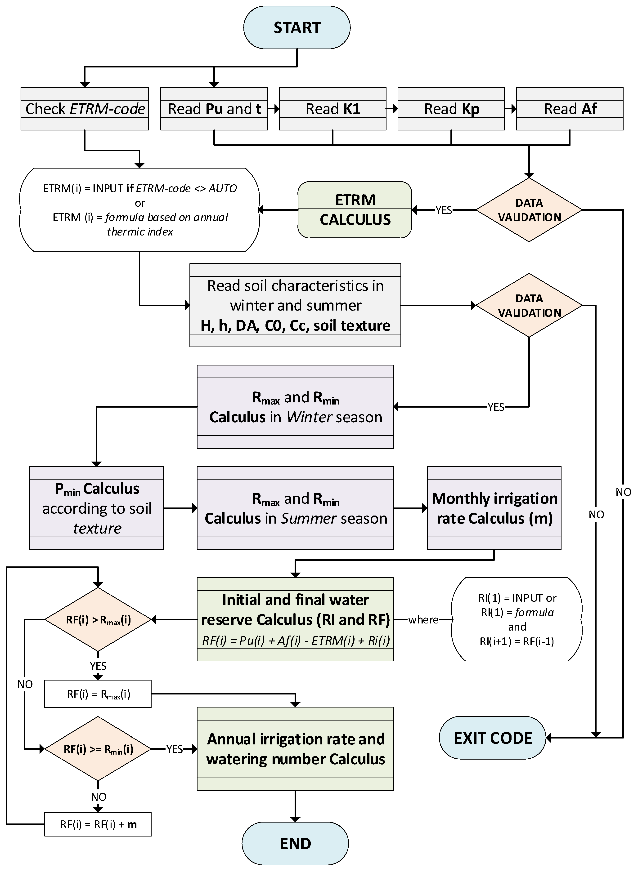
The flowchart of the study is presented in Figure 1.
The analysis steps (according to Figure 1) are:
- (a)
- Input data from the Excel files where they have been previously introduced. They are: monthly precipitation (Pu in the flowchart) and temperature series (t– in the flowchart), the series of the monthly coefficients K1 and Kp, and the series.The input data are validated by checking if the cells are filled in with numerical values. If not, the algorithm stops. Otherwise, it passes to the next step, as follows:
- (b)
- Read the soil characteristics, namely H, h, DA, , and corresponding to h and H from the worksheets where they were previously introduced. If all the values are numerical, and none is absent, the algorithm passes to step (c). Otherwise, it stops.
- (c)
- Compute and for winter;
- (d)
- Compute ;
- (e)
- Compute and for summer;
- (f)
- Compute the monthly irrigation rate;
- (g)
- Compute the initial and final water reserve for each month;
- (h)
- Compute the water application rate and the annual irrigation rate;
- (i)
- Display the results and the graphical representation.
3. Data Series
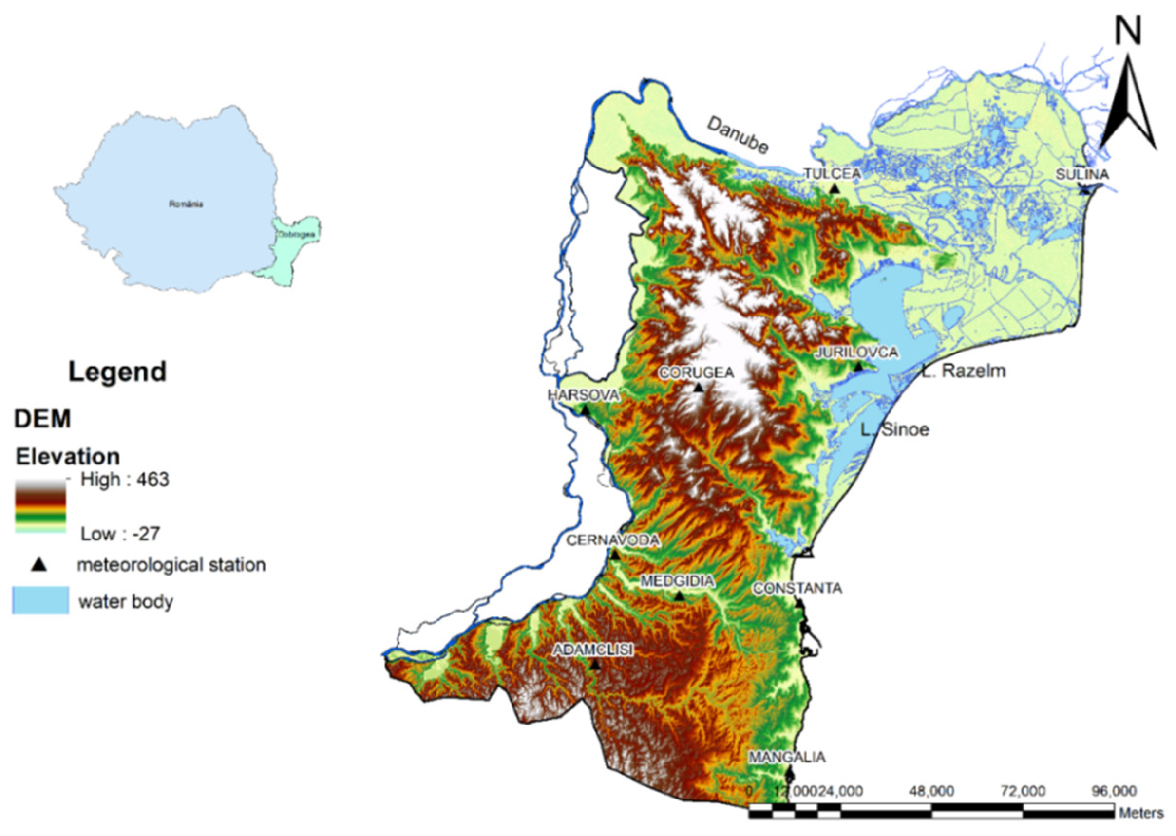
The climate in Romania is continuously changing, so the drought regions are becoming more arid. The Dobrogea region (Figure 2), situated in the south-eastern part of the country, is experiencing a more extended period without precipitation followed by short periods with high rainfalls. It was shown that the mean annual temperatures were augmented by 0.8 °C after 1997, and many rivers are drying up in summer. Increasing trends are noticed for the region’s maximum and minimum annual, summer, winter, and spring temperature series [37,38,39,40,41]. Therefore, the necessity of crop irrigation becomes more relevent than ever.
4. Implementation
The application was built in Microsoft Excel for graphics and VBA (Supplementary Materials S1 and S2) because these environments have also been employed for hydrological analysis, and the environment is easy to use [42,43,44,45,46].
The application’s structure allows the irrigation rate calculation for two locations (S1 and S2) and the comparison of results.
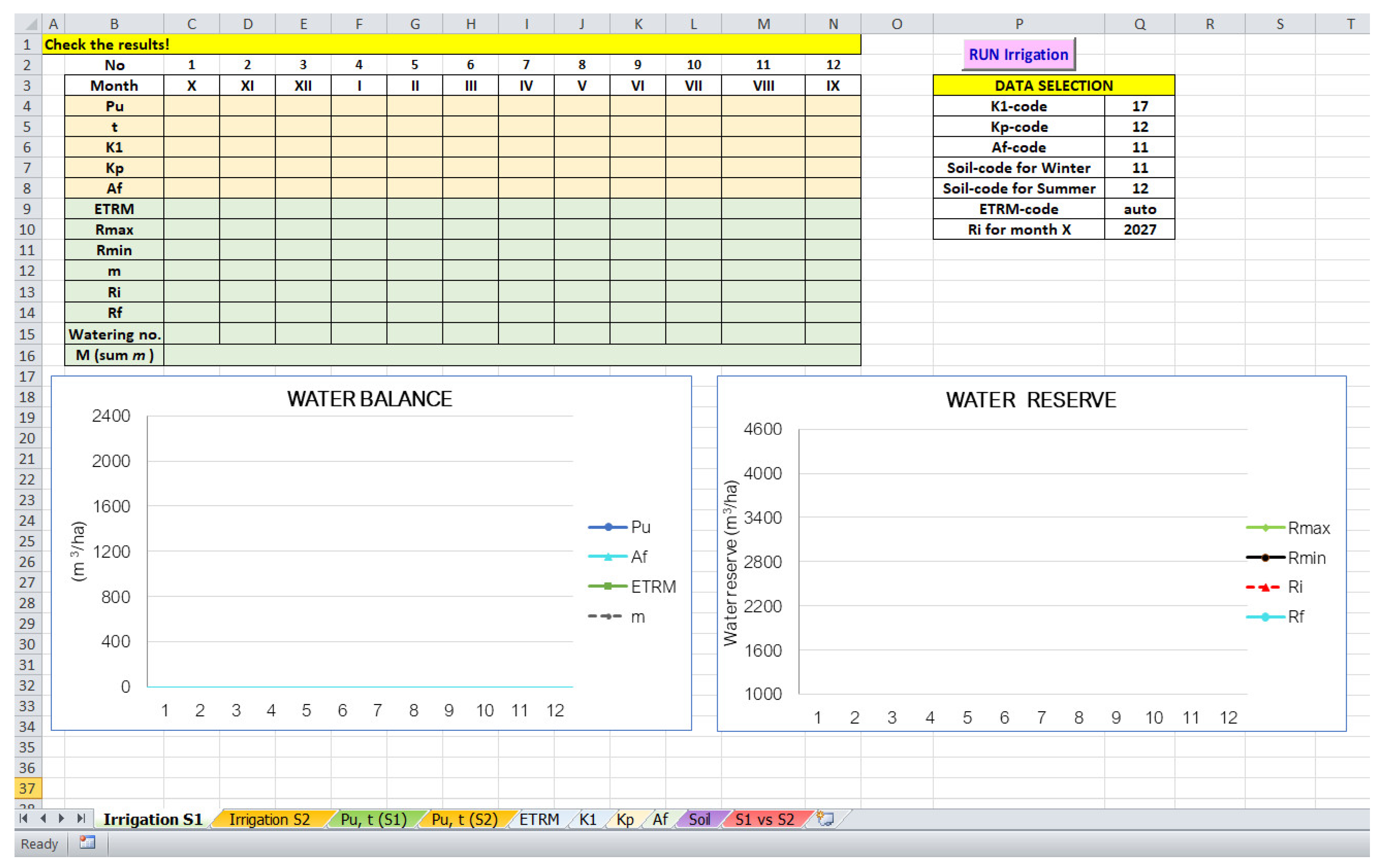
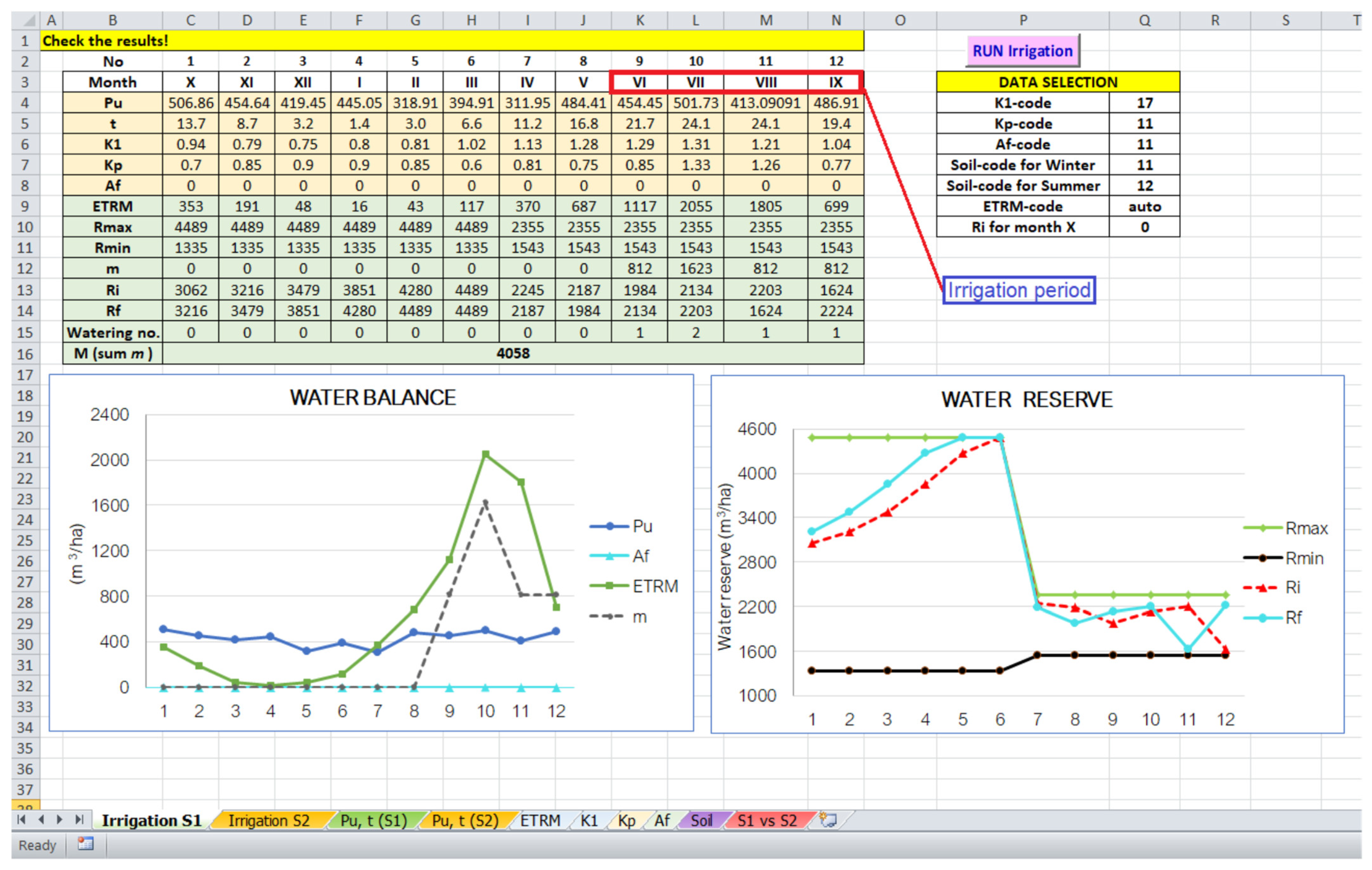
The main worksheets—“Irrigation S1” (Figure 4) and “Irrigation S2”—contain the work data for each site, the numerical results obtained, and the afferent charts obtained after running the algorithm.
Before running, the input data is entered in seven worksheets (“Pu, t (S1)”, “Pu, t (S2)”, “ETRM”, “K1”, “Kp”, “Af”, and “Soil”) that are simple and easy to populate by the user with data according to its need. They will be presented in the following section.
The software selects the values of interest through numerical codes, which correspond to the data sets entered by the user. In the “Irrigation S1” and “Irrigation S2” worksheets, the user indicates the codes (settable by him) in the table entitled “DATA SELECTION”.
The user will introduce into the cells Q4–Q11 the following codes:
- − in Q4—a code selected from the first column of the worksheet “K1”;
- − in Q5—a code selected from the first column of the worksheet “Kp”;
- − in Q6—a code selected from the first column of the worksheet “Af”;
- − in Q7—a code selected from the first column of the worksheet “Soil” corresponding to the winter season;
- − in Q8—a code selected from the first column of the worksheet “Soil” corresponding to the summer season;
- − in Q9—a code selected from the first column of the worksheet “ETRM” or “auto”;
- − in Q10—"0” or a value selected by the user.
Details will be provided in the following section.
The software takes the data corresponding to the codes from the worksheets “Pu, t (S1)” (Figure 5), “ETRM” (Figure 6), “K1” (Figure 7), “Kp” (Figure 8), “Af” (Figure 9), and “Soil” (Figure 10).
Initially, the cells from the rectangle C4–N4–N12–C12 in the “Irrigation S1” and “Irrigation S2” are empty. They are automatically filled in, concomitantly with the charts “WATER BALANCE” and “WATER RESERVE”, after running the code.
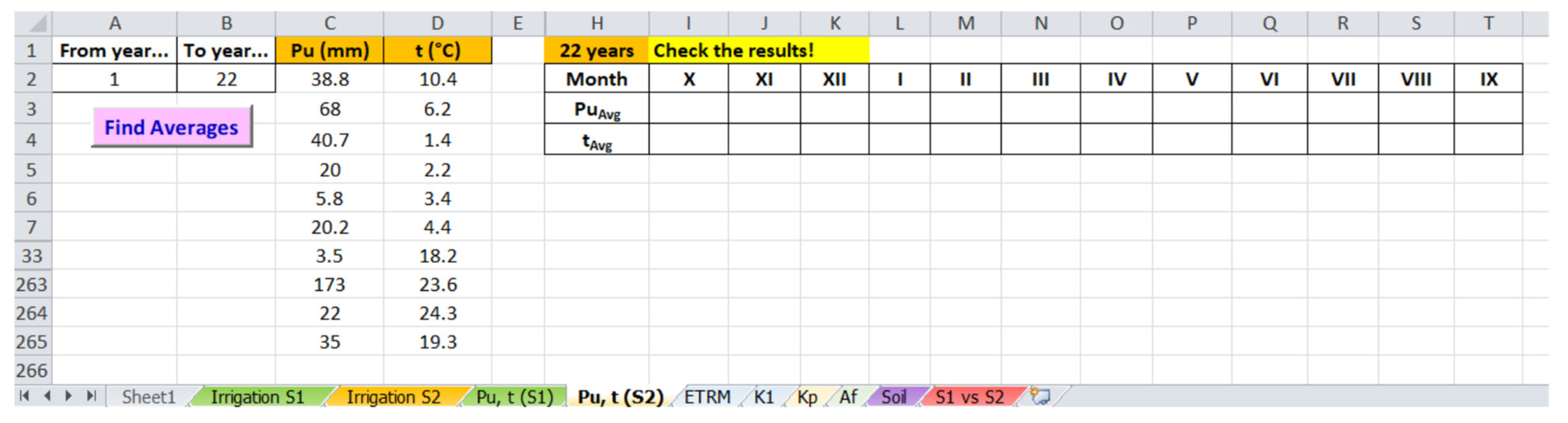
The monthly precipitation and temperature series are introduced in the worksheets “Pu, t (S1)” and “Pu, t (S2)” (Figure 5). The data are entered consecutively for an unlimited number of years for precipitation—in column C—and temperature—in D column D—separately. The worksheets (Figure 5) implement a 1–12 monthly average calculation module for both precipitation and temperature series. For performing the computation, the user can select all the years entered or a specific interval (for example, from year 5 to year 10) and press the button “Find Averages”.
The average values obtained are automatically displayed in the table next to the series: the cells I3–T3 for the average monthly precipitation and I4–T4 for the average monthly temperature. Cells are also automatically filled in the table from the main worksheets—“Irrigation S1” (for the series introduced in “Pu, t (S1)”) and “Irrigation S2” (for the series introduced in “Pu, t (S2)”)—namely the cells C4–N4 (for the average monthly precipitations) and C5–N5 (for the average monthly temperatures). These values are then employed to calculate the irrigation rates.
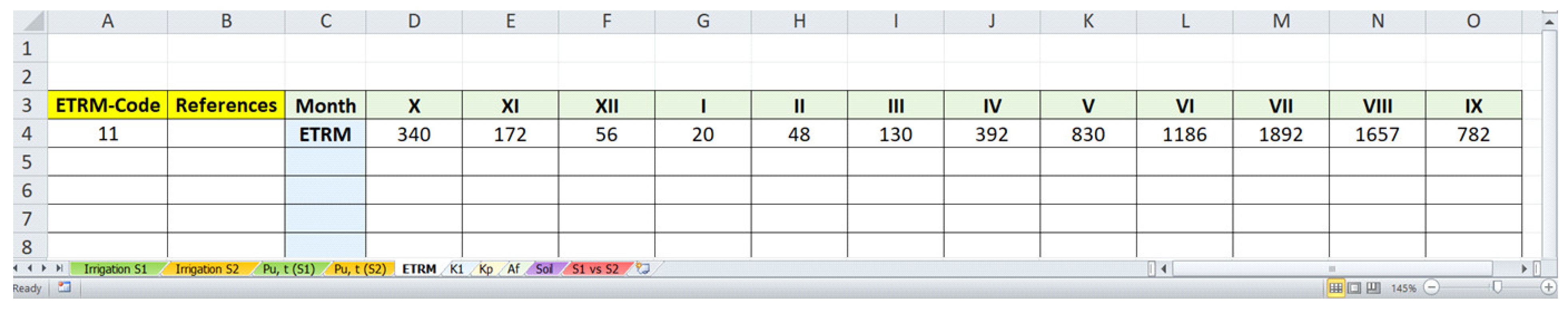
When running the program, the user may introduce the corresponding code (11 in the cell Q6 in the worksheets “Irrigation S1” and “Irrigation S2” from Figure 6) for ETRM. If the evapotranspiration is known (such as in Figure 6), and data were previously filled in the worksheet “ETRM”, the balance Equation (11) is computed using these values. If ETRM is unknown, the user must introduce the code “auto” in the cell Q6 in the worksheets “Irrigation S1” and “Irrigation S2”, and the ETRM is estimated using Equation (3).
To not restrict the use of the tool for some specific soil types, the series of coefficients , and are entered by the user in separate worksheets with the same names.
The “K1” worksheet (Figure 7) already contains some values corresponding to different northern latitudes, among which is the 45° north latitude utilized in the exemplification. The table can be filled with values for other latitudes and the corresponding K1 code (assigned by the user). Two different latitudes must have different K1 codes.
The “Kp” worksheet (Figure 8) contains some examples of values but can be filled with other values according to the crop and the region where it is cultivated. The user can assign the Kp code in column A and introduce any necessary description in column B.
In Figure 8 there are two types of crops—corn and alfalfa—and the corresponding coefficients for each location—Constanța and Tulcea. The values are filled in according to [35] for the two locations used for exemplification. For other locations and other crops, some values are provided in [33].
The K1 code and Kp code must be filled in the cells Q4 and Q5, respectively, from the main worksheets. When pressing the button “RUN Irrigation” from these worksheets, the corresponding and values are filled in automatically in the cells C6–N6 and C7–N7, respectively, in the main worksheets.
The “Af” worksheet (Figure 9) contains the groundwater’s supply values. The user can introduce them, and the code is filled in the cell Q6 from the main worksheets. When running the code, the values are automatically filled in the table from the “Irrigation S1” and “Irrigation S2” worksheets (the cells C8–Q8).
Figure 9 refers to the case when there is no water supply from the groundwater.
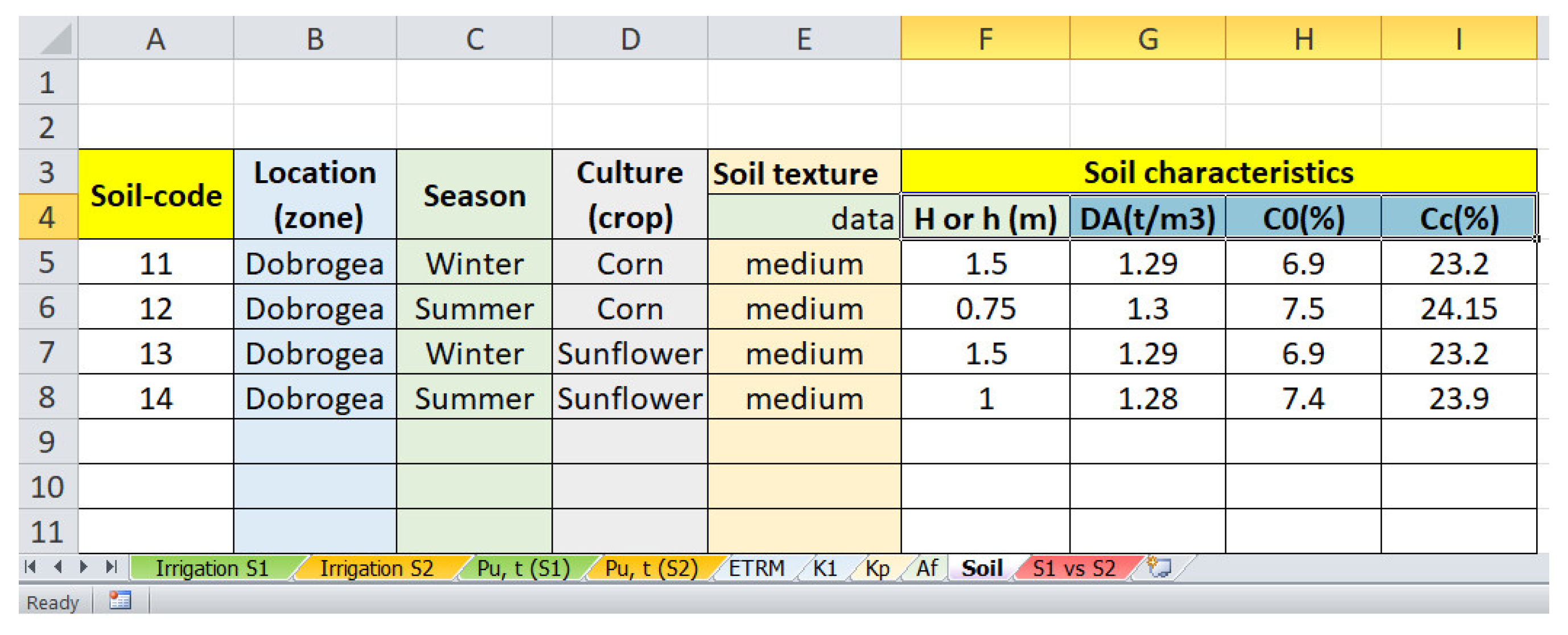
The “Soil” worksheet (Figure 10) contains the values of H, h, It must be filled with the corresponding values for each soil type and each season. Since the soil characteristics are specific to the season, crop, and soil type, the user should specify (in column B) the location, the crop (column D), and season (column E).
The irrigation rate and watering numbers (abbreviated by “Water no.” in the charts) are computed by pressing the command button in the “Irrigation S1” and “Irrigation S2” worksheets using Equations (1) and (2). The results and graphs are updated (the previous results are overwritten) both in the two main worksheets and in the comparison one (“S1 vs. S2”) (Figure 11).
5. Results
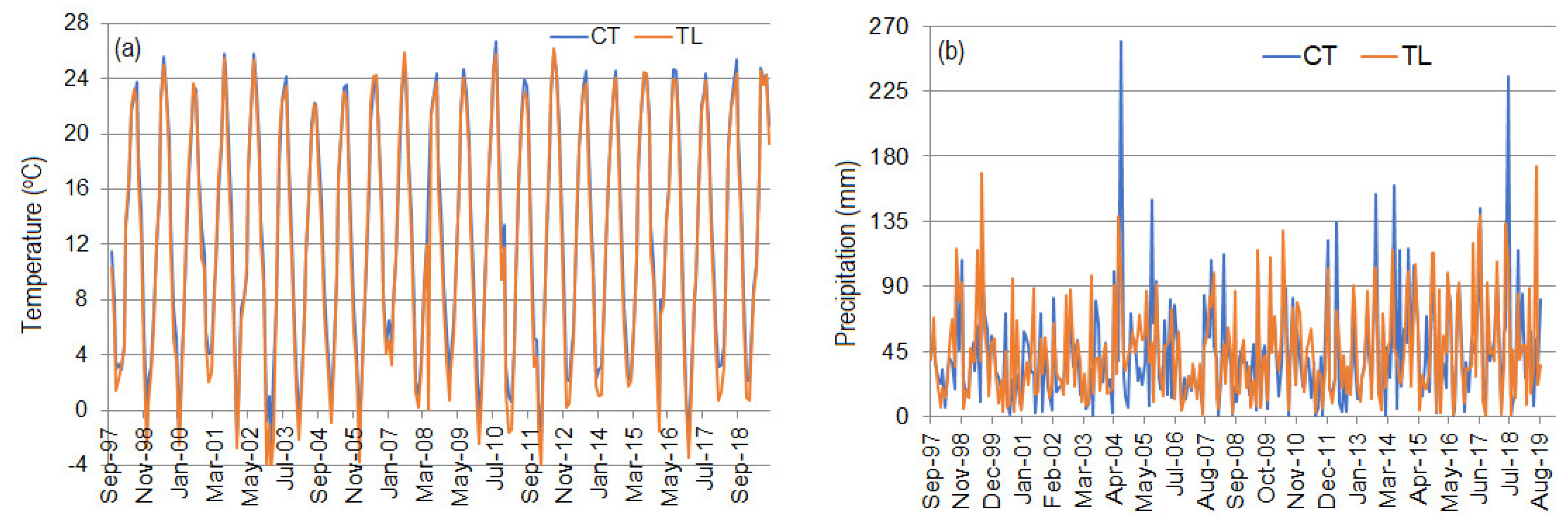
In the following, we exemplify how IrrigTool works, giving as input the monthly temperature and precipitation at Constanța and Tulcea (Romania) for 22 agricultural years (1998–2019). Given that the agricultural year starts in October (1 or month X in all the charts), the data series are introduced in the “Pu, t (S1)” and “Pu, t (S2)” worksheets. The chosen crop was corn.
Considering the geographical position of Romania, the K1 code represents the values of K1 corresponding to 45° northern latitude (Figure 7—C10).
The Kp code was chosen as 11 and 13 for CT and TL, respectively (Figure 8).
The water supply from groundwater was because the region is arid, so the Af code was set to 11 (Figure 9).
The Soil code (Figure 10) for winter (summer) was the same, 11 (12), given the same soil characteristics. The ETRM code was set to “auto”, so the ETRM was computed using Equation (3).
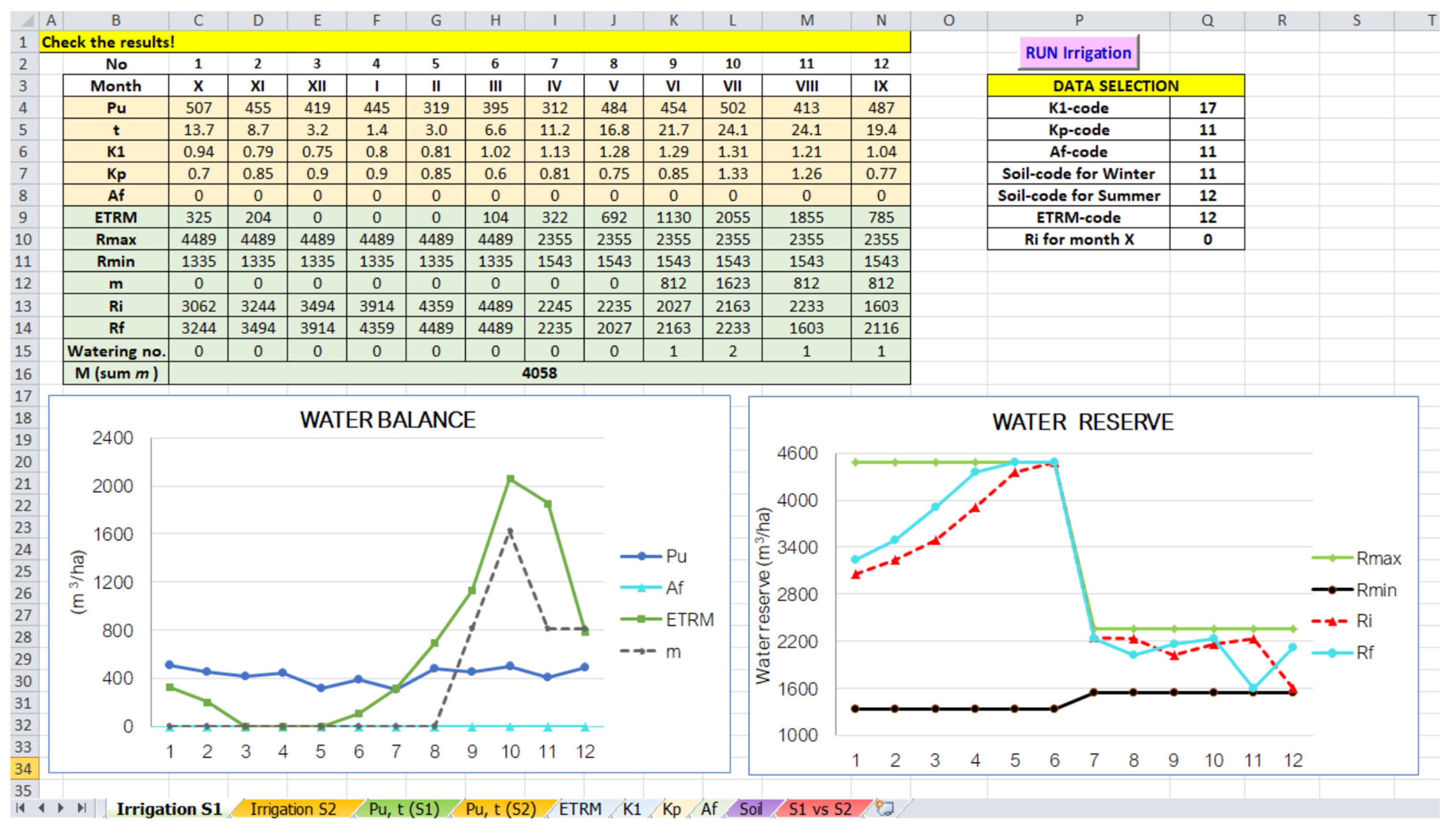
The initial water reserve in soil for October (Ri for month X) must be provided to start the computation. The user may introduce the value in the cell corresponding to “Ri for month X” from “Irrigation S1” and “Irrigation S2” or allow the software to compute it based on the formula (6) if “0” is inserted in that cell. The results obtained when the Ri for October is computed according to the methodology presented above are shown in Figure 12 (for CT) and Figure 13 (for TL), whereas their comparison is provided in Figure 14.
Row 15 in Figure 12 and Figure 13 contains the watering numbers. One watering must be applied in June, August, and September and two in July for both locations. The water application rate is m = 812 m3/ha (cells K12, M12, and N12, in Figure 12 and Figure 13). The value 1623 from cell L12 in Figure 12 and Figure 13 is equal to 2m. The irrigation rate is 4058 in both cases (row 16 in the left-hand side table in Figure 12 and Figure 13).
The “Water balance” charts (Figure 12 and Figure 13) illustrate the mean monthly precipitation, ETRM, , and m, whereas the second ones contain the water reserve (initial and final, maximum and minimum). The charts from Figure 14 summarize the findings for both locations.
The ETRMs are comparable at CT and TL. The initial and final water reserve is slightly higher at TL. The irrigation rate is the same at TL and CT. The watering should be applied the same month and in the same amount.
From Figure 12, Figure 13 and Figure 14, row 30, it results that during the first eight months of the agricultural year (October–May), it is not necessary to apply irrigation. In June, August, and September, one watering should be applied (812 m3/ha). In July, watering should be applied twice (a total of 1624 m3/ha).
This aspect is emphasized in Figure 12 and Figure 13, the bottom left chart, by the black dotted curves and in Figure 14, the top chart, by the yellow continuous curve (for CT) and the black dotted curve (for TL).
Given that the watering distribution depends on the initial soil reserve in October, the user may run the algorithm many times, at each run considering the initial water reserve in soil in October to be equal to the final water reserve in September in the previous run (and introducing manually this value in the cell “Ri for month X”).
6. Discussion
First, we compared the irrigation rate obtained using the Thornthwaite equation with the results obtained using the measured ETRM in the neighborhood of Constanța (at Mamaia). We mention that the procedure followed in Romania is that the ETRM is measured only for nine months, from March to November, so the rest of the values are considered to be zero. Therefore, IrrigTool was run with the ETRM code 12 in the worksheet “ETRM” (Figure 15). The output is shown in Figure 16.
There are no significant differences between the computed and measured ETRM values—cells C9–E9 in Figure 12 and Figure 16 and the watering numbers are the same (one in June, August, and September and two in July).
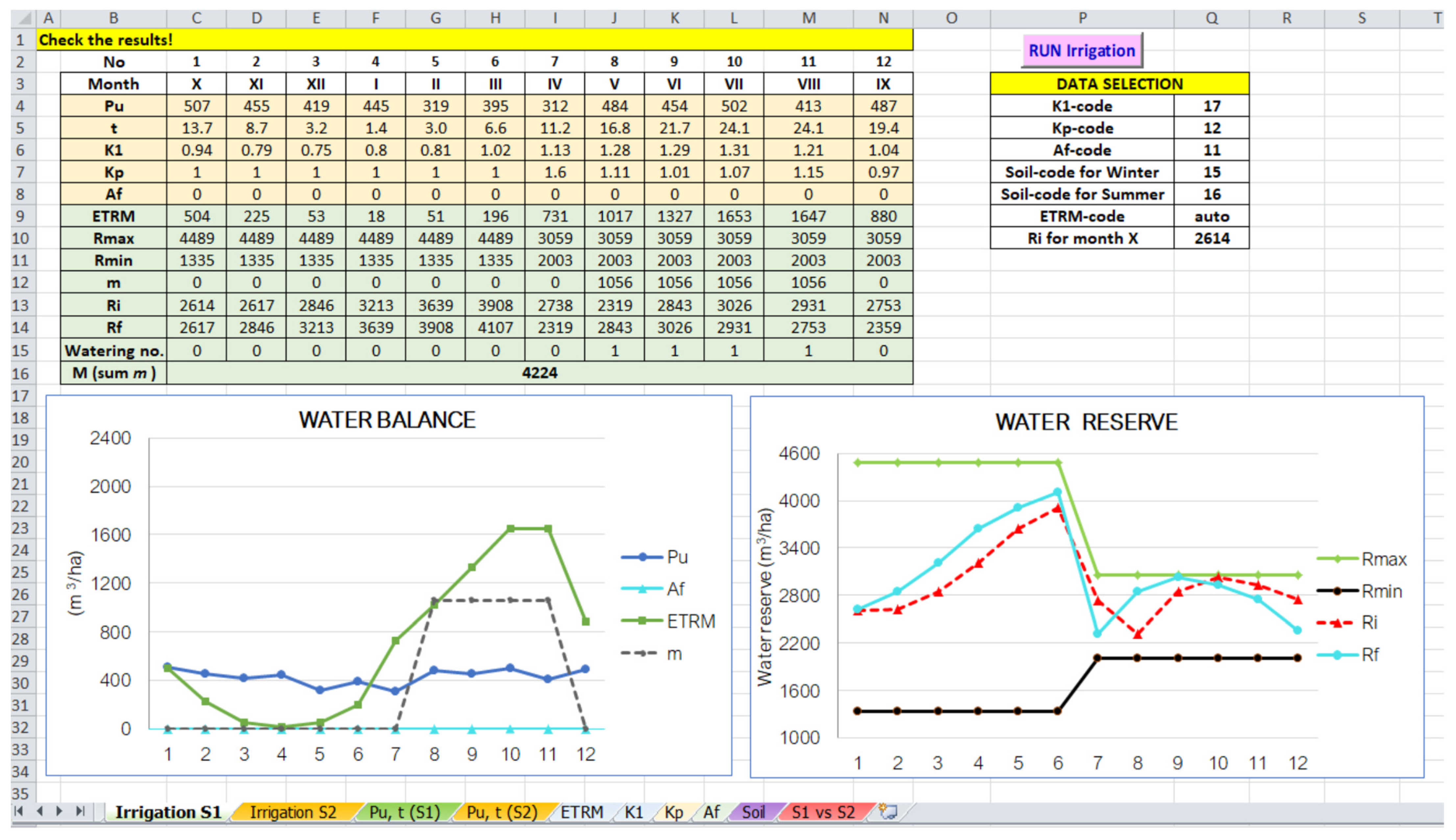
In the previous section, we indicated that the irrigation rate depends on the crop. To illustrate this assertion, we considered the crop alfalfa with the Kp code 12 (alfalfa). In this case, the soil code must be modified as well. In this case, it will be 15 for summer and 16 for summer (Figure 17).
The watering number has a different distribution: one in June and July and two in August. The irrigation rate is 4224 m3/ha because, in this case, m = 1056 m3/ha.
It was also mentioned that the irrigation rate depends on the initial water reserve in the soil. To exemplify, let us consider the same settings as in Figure 17, with Ri in the month 1 = Rmin in the month IX (2614 m3/ha), and run the algorithm. In this case, one watering should be applied in from May to July. The irrigation rate will remain the same: 4224 m3/ha (Figure 18).
If the water reserve in the soil is known, it is indicated to use its value to better estimate the irrigation rate.
7. Conclusions
This article presented a new tool, IrrigTool, designed for computing the irrigation rate based on the Thornthwaite equation for ETRM. It is implemented in VBA and Excel and is easy to use without knowledge of the formula implementation. The user can introduce the data series in different worksheets whereby, during the computation, the programs import the data into the main worksheets. The output for two different data sets can be compared as series of numbers and graphically.
This tool’s main advantage is that it permits the user to use either the Thornthwaite equation for ETRM computation or to manually fill in the recorded values of ETRM. Manually selecting or automatically computing the initial water reserve for the first month of the agricultural year is also permitted based on the available data. Moreover, there is no limitation related to the climatic conditions. The tool is user-friendly because it does not require programming skills but only basic knowledge of Excel.
A disadvantage of this tool is that the irrigation rate is computed only using the Thornthwaite equation (when ETRM is not known) and does not provide a comparison with another method. Therefore, in future work, we have the following goals: (a) to add a module that computes the ETRM by the Penman–Monteith equation and (b) to add a module to compare the irrigation rates computed based on the Thornthwaite and the Penman–Monteith equations.
Supplementary Materials
The following supporting information can be downloaded at: https://www.mdpi.com/article/10.3390/w14152399/s1, Excel–VBA application: IrrigTool. S1. The VBA code, S2. The VBA–Excel Application.
Author Contributions
Conceptualization, A.B. and C.E.M.; methodology, A.B. and C.E.M.; software, C.Ș.D.; validation, A.B. and C.Ș.D.; formal analysis, A.B. and C.Ș.D.; investigation, A.B.; data curation, A.B.; writing—original draft preparation, A.B.; writing—review and editing, A.B. and C.Ș.D.; visualization, C.Ș.D.; supervision, A.B.; project administration, A.B.; funding acquisition, A.B. All authors have read and agreed to the published version of the manuscript.
Funding
This research received no external funding.
Data Availability Statement
Not applicable.
Conflicts of Interest
The authors declare no conflict of interest.
References
- Bărbulescu, A.; Dumitriu, C.Ș. Assessing the water quality by statistical methods. Water 2021, 13, 1026. [Google Scholar] [CrossRef]
- Bărbulescu, A.; Nazzal, Y.; Howari, F. Assessing the groundwater quality in the Liwa area, the United Arab Emirates. Water 2020, 12, 2816. [Google Scholar] [CrossRef]
- Gómez, V.M.R.; Gutiérrez, M.; Haro, B.N.; López, D.N.; Herrera, M.T.A. Groundwater quality impacted by land use/land cover change in a semiarid region of Mexico. Groundw. Sustain. Dev. 2017, 5, 160–167. [Google Scholar] [CrossRef]
- Towards a Water and Food Secure Future. Critical Perspectives for Policy-Makers, Food and Agriculture Organization of The United Nations Rome. Revised Reprint World Water Council Marseille. 2015. Available online: http://www.fao.org/3/i4560e/i4560e.pdf (accessed on 9 October 2021).
- United Nations World Water Assessment Programme. The United Nations World Water Development Report 2015: Water for a Sustainable World; UNESCO: Paris, French, 2015; Available online: http://www.unesco.org/new/en/natural-sciences/environment/water/wwap/wwdr/2015-water-for-a-sustainable-world/ (accessed on 9 October 2021).
- Hargreaves, G.H.; Riley, J.P.; Sikka, A. Influence of climate on Irrigation. Can. Water Resour. J. 1993, 18, 53–59. [Google Scholar] [CrossRef] [Green Version]
- Li, Y.; Li, J.; Gao, L.; Tian, Y. Irrigation has more influence than fertilization on leaching water quality and the potential environmental risk in excessively fertilized vegetable soils. PLoS ONE 2018, 13, e0204570. [Google Scholar] [CrossRef] [PubMed]
- Haddeland, I.; Lettenmaier, D.P.; Skaugen, T. Effects of irrigation on the water and energy balances of the Colorado and Mekong river basins. J. Hydrol. 2006, 324, 210–223. [Google Scholar] [CrossRef]
- de Rosnay, P.; Polcher, J.; Laval, K.; Sabre, M. Integrated parameterization of irrigation in the land surface model ORCHIDEE: Validation over Indian Peninsula. Geophys. Res. Lett. 2003, 30, 1986. [Google Scholar] [CrossRef]
- Lobell, D.; Bala, G.; Mirin, A.; Phillips, T.; Maxwell, R.; Rotman, R. Regional Differences in the Influence of Irrigation on Climate. J. Clim. 2009, 22, 2248–2255. [Google Scholar] [CrossRef]
- Schaible, G.D.; Aillery, M.P. Water Conservation in Irrigated Agriculture: Trends and Challenges in the Face of Emerging Demands. Econ. Inform. Bull. 2012, 99, 67. Available online: https://www.ers.usda.gov/publications/pub-details/?pubid=44699 (accessed on 20 September 2021). [CrossRef] [Green Version]
- Huang, Q.; Xu, Y.; Kovacs, K.; West, G. Analysis of factors that influence the use of irrigation technologies and water management practices in Arkansas. J. Agric. Appl. Econ. 2017, 49, 159–185. [Google Scholar] [CrossRef] [Green Version]
- Henggeler, J. Software Programs Currently Available for Irrigation Scheduling. Available online: https://www.irrigation.org/IA/FileUploads/IA/Resources/TechnicalPapers/2002/SoftwareProgramsCurrentlyAvailableForIrrigationScheduling.pdf (accessed on 9 October 2021).
- Bos, M.G.; Kselik, R.A.L.; Allen, R.G.; Molden, D.J. Water Requirements for Irrigation and the Environment; Springer: Dordrecht, The Netherlands, 2009. [Google Scholar]
- CRIWAR 3.0. Available online: https://www.bos-water.nl/links-downloads (accessed on 10 July 2022).
- Allen, R.G.; Pereira, L.S.; Raes, D.; Smith, M. Crop Evapotranspiration-Guidelines for Computing Crop Water Requirements-FAO Irrigation and Drainage Paper 56, FAO—Food and Agriculture Organization of the United Nations Rome. 1998. Available online: http://www.fao.org/3/x0490e/x0490e00.htm (accessed on 9 October 2021).
- Allen, R.G.; Pereira, L.S.; Raes, D.; Smith, M. FAO Irrigation and Drainage Paper no. 56, Evapotranspiration (Guidelines for Computing Crop Water Requirements). Available online: http://www.climasouth.eu/sites/default/files/FAO%2056.pdf (accessed on 10 May 2021).
- Raes, D. The ETo Calculator. Evapotranspiration from a Reference Surface. Available online: https://www.ipcinfo.org/fileadmin/user_upload/faowater/docs/ReferenceManualV32.pdf (accessed on 8 May 2021).
- Penman-Montieth, E.T. Worksheet with Solar Estimate and Equation Instructions. Available online: https://extension.umaine.edu/blueberries/factsheets/irrigation/penman-montieth-et-worksheet-with-solar-estimate/ (accessed on 8 May 2021).
- CROPWAT 8.0 for Windows. Available online: https://www.fao.org/land-water/databases-and-software/cropwat/en/ (accessed on 5 May 2021).
- Donker, N.H.W. WTRBLN: A computer program to calculate water balance. Comput. Geosci. 1987, 13, 95–122. [Google Scholar] [CrossRef]
- Sellinger, C.E. Computer Program for Estimating Evapotranspiration Using the Thornthwaite Method. In NOAA Technical Memorandum ERL GLERL-101; United States Department of Commerce: Washington, DC, USA, 1996. [Google Scholar]
- Armiraglio, S.; Cerabolini, B.; Gandellini, F.; Gandini, P.; Andreis, C. Calcolo informatizzato del bilancio idrico del suolo. Nat. Bresciana. Ann. Mus. Civ. Sci. Nat. Brescia 2003, 33, 209–216. [Google Scholar]
- McCabe, G.J.; Markstrom, S.L. A Monthly Water-Balance Model Driven by A Graphical User Interface; Open-File Report 2007-1088; U.S. Geological Survey: Reston, VA, USA, 2007; 6p. [CrossRef] [Green Version]
- Mammoliti, E.; Fronzi, D.; Mancini, A.; Valigi, D.; Tazioli, A. WaterbalANce, a WebApp for Thornthwaite–Mather water balance computation: Comparison of applications in two European watersheds. Hydrology 2021, 8, 34. [Google Scholar] [CrossRef]
- Droogers, P.; Immerzeel, W.W.; Lorite, I.J. Estimating actual irrigation application by remotely sensed evapotranspiration observations. Agric. Water Manag. 2010, 97, 1351–1359. [Google Scholar] [CrossRef]
- Olivera-Guerra, L.; Merlin, O.; Er-Raki, S. Irrigation retrieval from Landsat optical/thermal data integrated into a crop water balance model: A case study over winter wheat fields in a semi-arid region. Remote Sens. Environ. 2020, 239, 111627. [Google Scholar] [CrossRef] [Green Version]
- Brocca, L.; Tarpanelli, A.; Filippucci, P.; Dorigo, W.; Zaussinger, F.; Gruber, A.; Fernández-Prieto, D. How much water is used for irrigation? A new approach exploiting coarse resolution satellite soil moisture products. Int. J. Appl. Earth Obs. Geoinf. 2018, 73, 752–766. [Google Scholar] [CrossRef]
- Bretreger, D.; Yeo, I.Y.; Hancock, G. Quantifying irrigation water use with remote sensing: Soil water deficit modelling with uncertain soil parameters. Agric. Water Manag. 2022, 260, 107299. [Google Scholar] [CrossRef]
- Foster, T.; Mieno, T.; Brozović, N. Satellite-Based monitoring of irrigation water use: Assessing measurement errors and their implications for agricultural water management policy. Water Resour. Resear. 2020, 56, e2020WR028378. [Google Scholar] [CrossRef]
- CAWATERinfo. Irrigation and Water Application Rate. Available online: http://www.cawater-info.net/bk/4-2-1-1-3-3_e.htm (accessed on 7 June 2022).
- Roșu, L. Land Ameliorations; Ovidius University Press: Constanta, Romania, 1999. (In Romanian) [Google Scholar]
- Pleșa, I.; Florescu, G.; Mușat, I. Land Amelioration; Editura Didactică și Pedagogică: Bucharest, Romania, 1967. (In Romanian) [Google Scholar]
- Ștefan, V.; Bechet, S.; Tomiță, O.; Titz, L. Land Amelioration; Editura Didactică și Pedagogică: Bucharest, Romania, 1981. (In Romanian) [Google Scholar]
- Cismaru, C.; Gabor, V. Irrigation. Arrangements, Rehabilitations and Modernizations; Editura POLITEHNIUM: Iasi, Romania, 2004. (In Romanian) [Google Scholar]
- Cazacu, E.; Dorobantu, M.; Georgescu, I.; Sarbu, E. Irrigations Arrangements; Ceres: Bucharest, Romania, 1982. (In Romanian) [Google Scholar]
- Bărbulescu, A. Models for temperature evolution in Constanta area (Romania). Rom. J. Phys. 2016, 61, 676–686. [Google Scholar]
- Bărbulescu, A.; Deguenon, J. About the variations of precipitation and temperature evolution in the Romanian Black Sea Littoral. Rom. Rep. Phys. 2015, 67, 625–637. [Google Scholar]
- Bărbulescu, A.; Dumitriu, C.S.; Maftei, C. On the Probable Maximum Precipitation Method. Rom. J. Phys. 2022, 67, 801. [Google Scholar]
- Bărbulescu, A.; Maftei, C. Statistical approach of the behavior of Hamcearca River (Romania). Rom. Rep. Phys. 2021, 73, 703. [Google Scholar]
- Maftei, C.; Bărbulescu, A.; Rugină, S.; Nastac, C.D.; Dumitru, I.M. Analysis of the arbovirosis potential occurence in Dobrogea, Romania. Water 2021, 13, 374. [Google Scholar] [CrossRef]
- Bărbulescu, A.; Maftei, C.; Dumitriu, C. The modeling of the climatic process that participates at the sizing of an irrigation system. Appl. Comput. Math. 2002, 2048, 11–20. [Google Scholar]
- Halford Tools. Available online: https://halfordhydrology.com/tools/ (accessed on 29 June 2022).
- GR2M Model. Available online: https://webgr.inrae.fr/en/models/monthly-model-gr2m/ (accessed on 29 June 2022).
- GR4J_FR. Available online: https://webgr.inrae.fr/modeles/journalier-gr4j-2/ (accessed on 29 June 2022).
- Niazkar, M. An Excel VBA-based educational module for bed roughness predictors. Comput. Appl. Eng. Educ. 2021, 29, 1051–1060. [Google Scholar] [CrossRef]
- Miller, S. Handbook for Agrohydrology; Natural Resources Institute: London, UK, 1994; Available online: http://www.nzdl.org/cgi-bin/library.cgi?e=d-00000-00---off-0hdl--00-0----0-10-0---0---0direct-10---4-------0-1l--11-en-50---20-about---00-0-1-00-0-0-11-1-0utfZz-8-00&cl=CL3.37&d=HASH3b4d99e5f9716ab628b9b2>=2 (accessed on 7 June 2022).
Figure 1.
Flowchart (the variables are denoted in concordance with the coding).

Figure 2.
The map of Dobrogea [41].
Figure 2.
The map of Dobrogea [41].

Figure 3.
Monthly average (a) temperature and (b) precipitation series recorded at Constanța (CT) and Tulcea (TL).
Figure 3.
Monthly average (a) temperature and (b) precipitation series recorded at Constanța (CT) and Tulcea (TL).

Figure 4.
The “Irrigation S1” worksheet.

Figure 5.
The “Pu, t (S1)” sheet.

Figure 6.
The “ETRM” worksheet.


Figure 8.
The “Kp” worksheet. Data are reproduced from [35], p. 41.
Figure 8.
The “Kp” worksheet. Data are reproduced from [35], p. 41.

Figure 9.
The “Af” worksheet.

Figure 10.
The “Soil” worksheet.

Figure 11.
The “S1 vs. S2” worksheet.

Figure 12.
Computation results for CT.

Figure 13.
Computation results for TL.

Figure 14.
Comparison of the results for CT and TL (from the worksheet “S1 vs. S2”).

Figure 15.
Average ETRM values in the neighborhood of CT, at Mamaia (5 km from CT).

Figure 16.
Output of running the algorithm using ETRM recorded at Mamaia (5 km from CT).

Figure 17.
Output for alfalfa at CT, computed using the Thornthwaite equation.

Figure 18.
Output for alfalfa at CT, computed by the Thornthwaite equation, with Ri = 2614 m3/ha.


Table 1.
Basic statistics of the CT and TL monthly series used for exemplification.
| Series | Max | Min | Mean | Median | Std. Dev. | Coef. of Variation | Skewness | Kurtosis |
|---|---|---|---|---|---|---|---|---|
| CT precipitation | 259.20 | 0.30 | 43.27 | 36.00 | 36.53 | 0.84 | 1.96 | 6.95 |
| TL precipitation | 173.00 | 0.00 | 44.83 | 37.35 | 33.91 | 0.76 | 1.06 | 0.85 |
| CT temperature | 26.70 | −0.20 | 12.83 | 12.60 | 8.17 | 0.64 | −0.03 | −1.29 |
| TL temperature | 26.20 | −4.50 | 12.08 | 11.65 | 8.60 | 0.71 | −0.06 | −1.28 |
Publisher’s Note: MDPI stays neutral with regard to jurisdictional claims in published maps and institutional affiliations. |
© 2022 by the authors. Licensee MDPI, Basel, Switzerland. This article is an open access article distributed under the terms and conditions of the Creative Commons Attribution (CC BY) license (https://creativecommons.org/licenses/by/4.0/).
Share and Cite
MDPI and ACS Style
Dumitriu, C.Ș.; Bărbulescu, A.; Maftei, C.E. IrrigTool—A New Tool for Determining the Irrigation Rate Based on Evapotranspiration Estimated by the Thornthwaite Equation. Water 2022, 14, 2399. https://doi.org/10.3390/w14152399
AMA Style
Dumitriu CȘ, Bărbulescu A, Maftei CE. IrrigTool—A New Tool for Determining the Irrigation Rate Based on Evapotranspiration Estimated by the Thornthwaite Equation. Water. 2022; 14(15):2399. https://doi.org/10.3390/w14152399
Chicago/Turabian StyleDumitriu, Cristian Ștefan, Alina Bărbulescu, and Carmen Elena Maftei. 2022. "IrrigTool—A New Tool for Determining the Irrigation Rate Based on Evapotranspiration Estimated by the Thornthwaite Equation" Water 14, no. 15: 2399. https://doi.org/10.3390/w14152399
Note that from the first issue of 2016, this journal uses article numbers instead of page numbers. See further details here.