
Application of Analytical Hierarchy Process and Geophysical Method for Groundwater Potential Mapping in the Tata Basin, Morocco


 , ,
, ,  , ,
, , 
Abstract
:1. Introduction
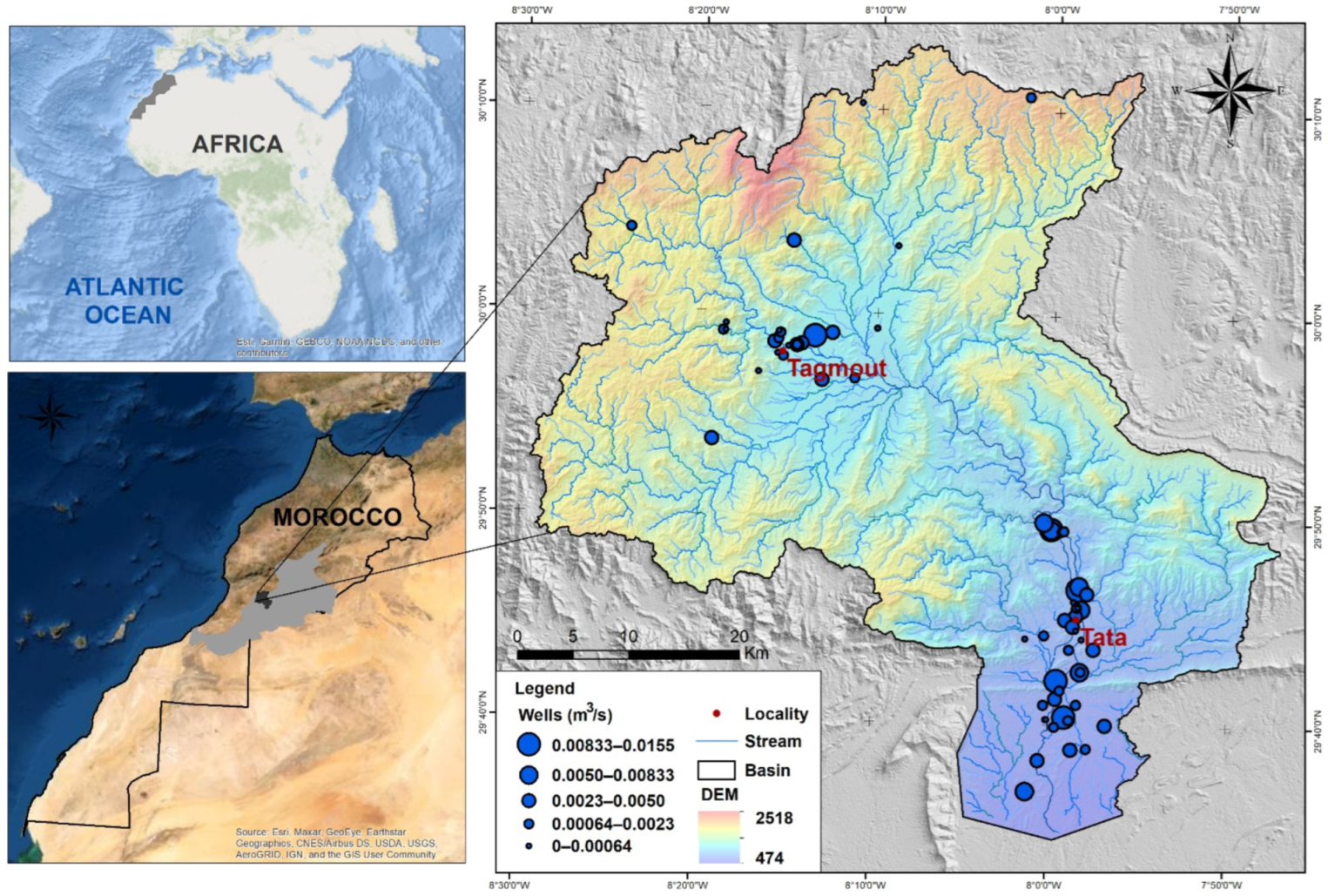
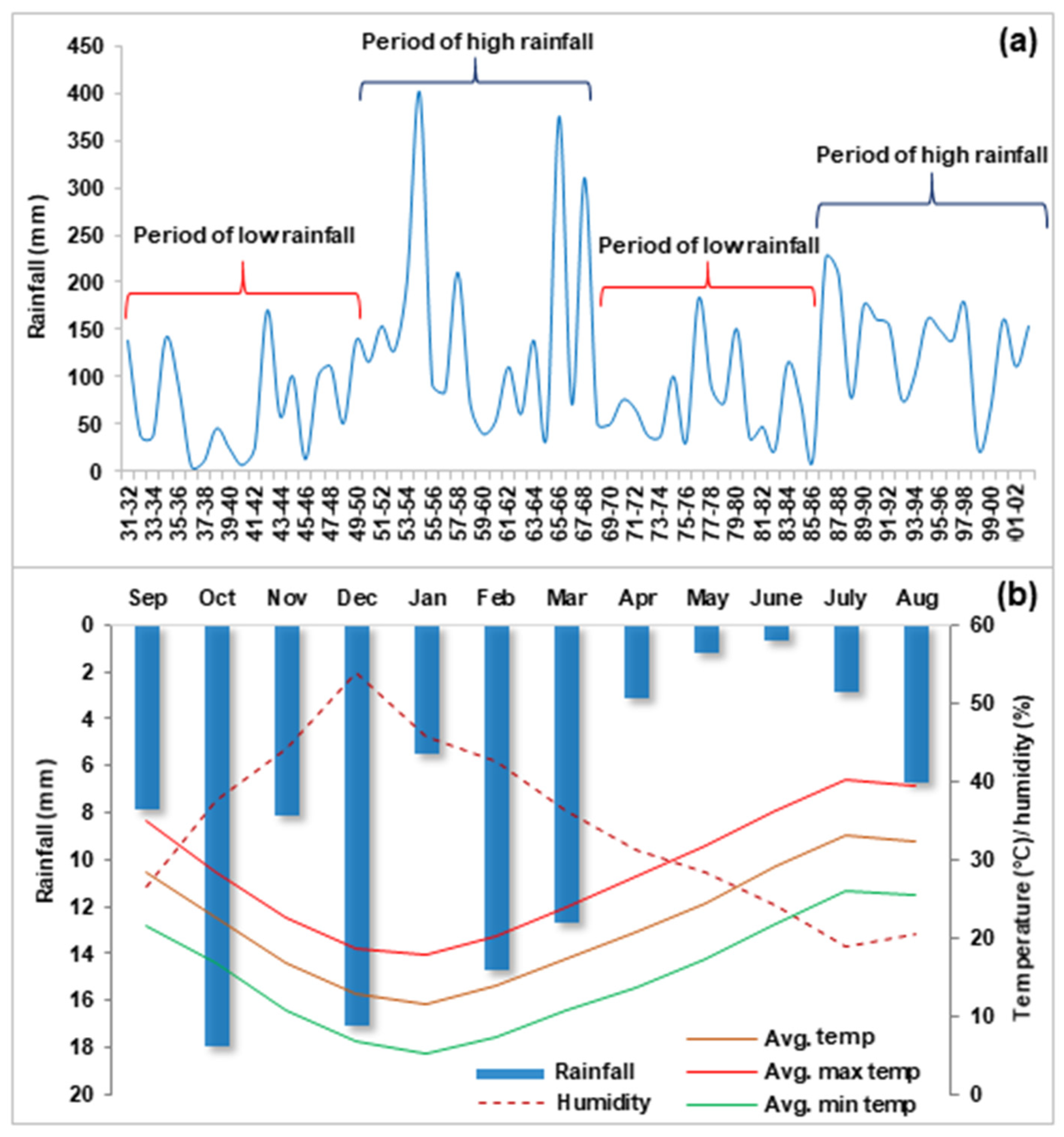
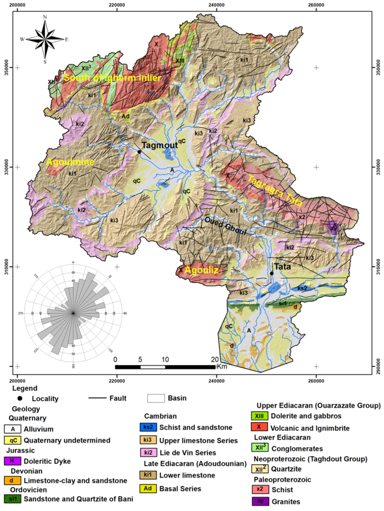
2. Study Area
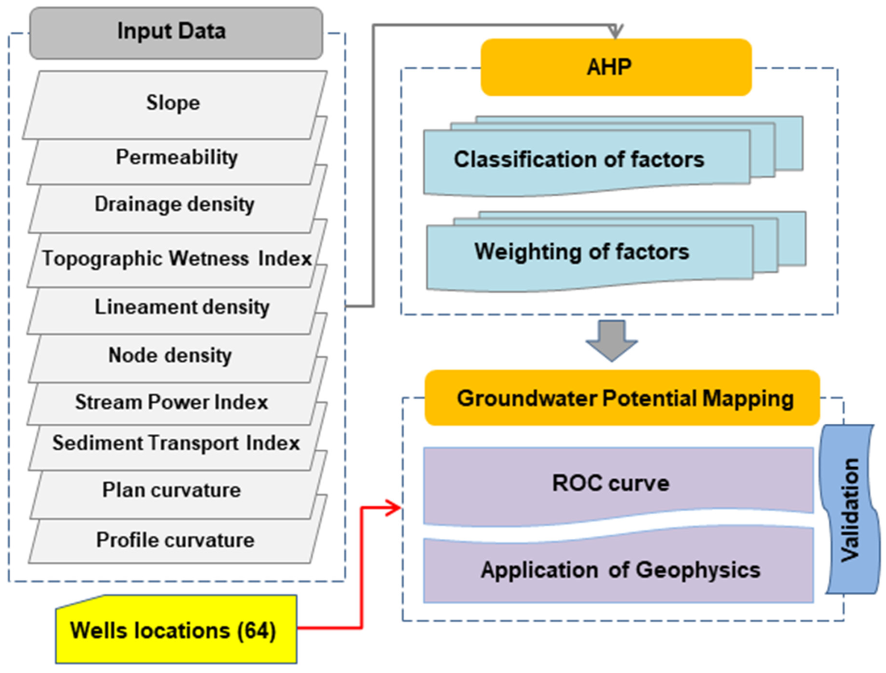
3. Materials and Methods
3.1. Analytical Hierarchy Process (AHP) Model
3.2. Determination of Decision Factors
3.3. Development of Decision Factor Maps
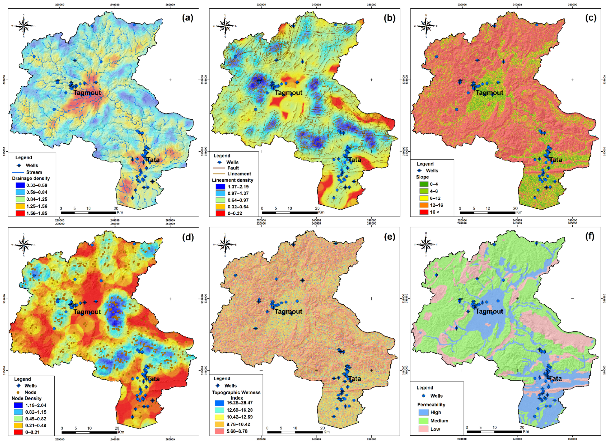
3.3.1. Drainage Density (DD)
3.3.2. Lineaments Density (LD)
3.3.3. Slope (SL)
3.3.4. Node Density (ND)
3.3.5. Topographic Wetness Index (TWI)
3.3.6. Permeability (PER)
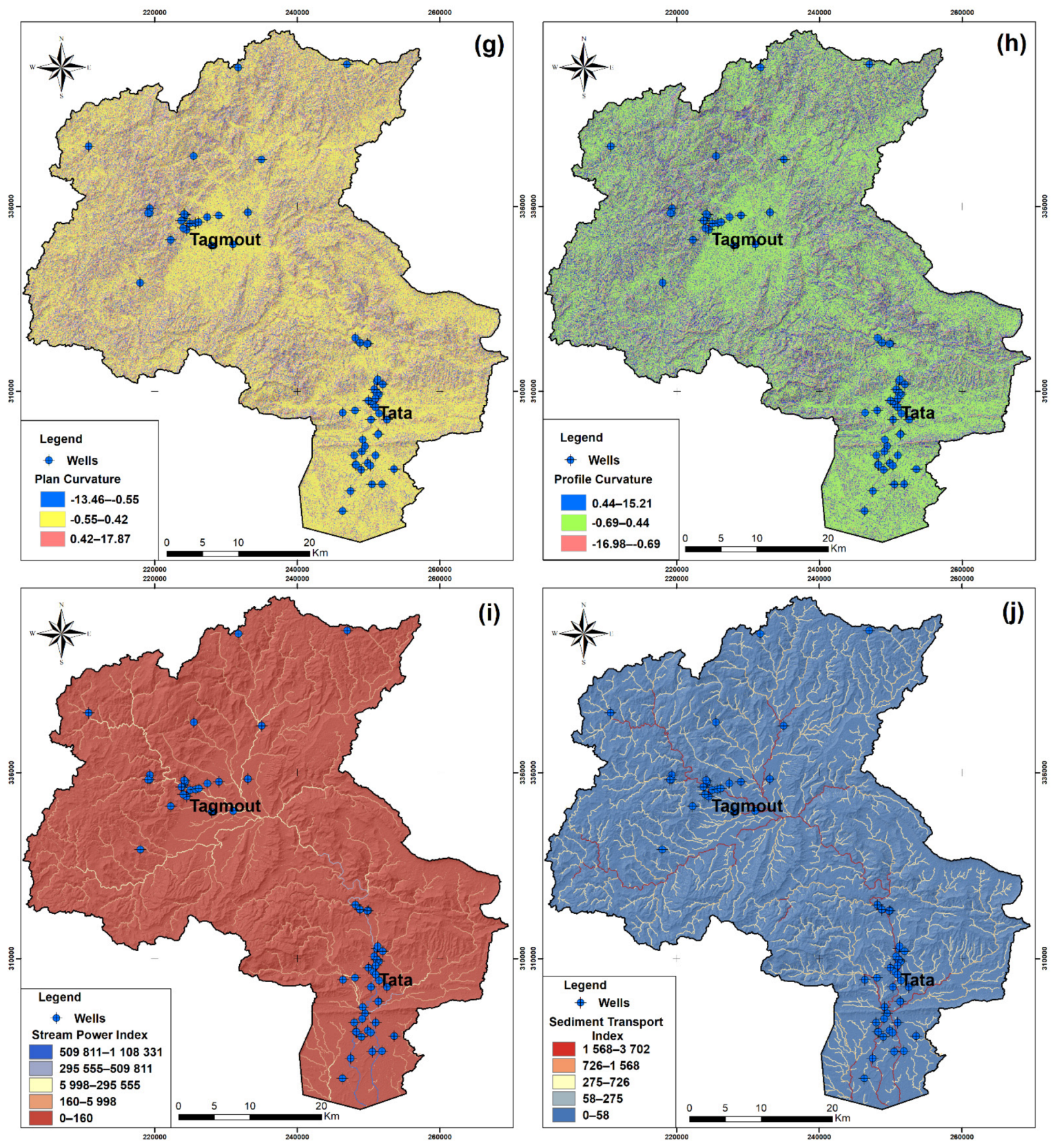
3.3.7. Plan Curvature (PLC)
3.3.8. Profile Curvature (PRC)
3.3.9. Stream Power Index (SPI)
3.3.10. Sediment Transport Index (STI)
3.4. Classification and Standardization of Factors
3.5. Weighting of the Deciding Factors
3.6. Determination of the GWPM
3.7. Validation of the GWPM
4. Results and Discussion
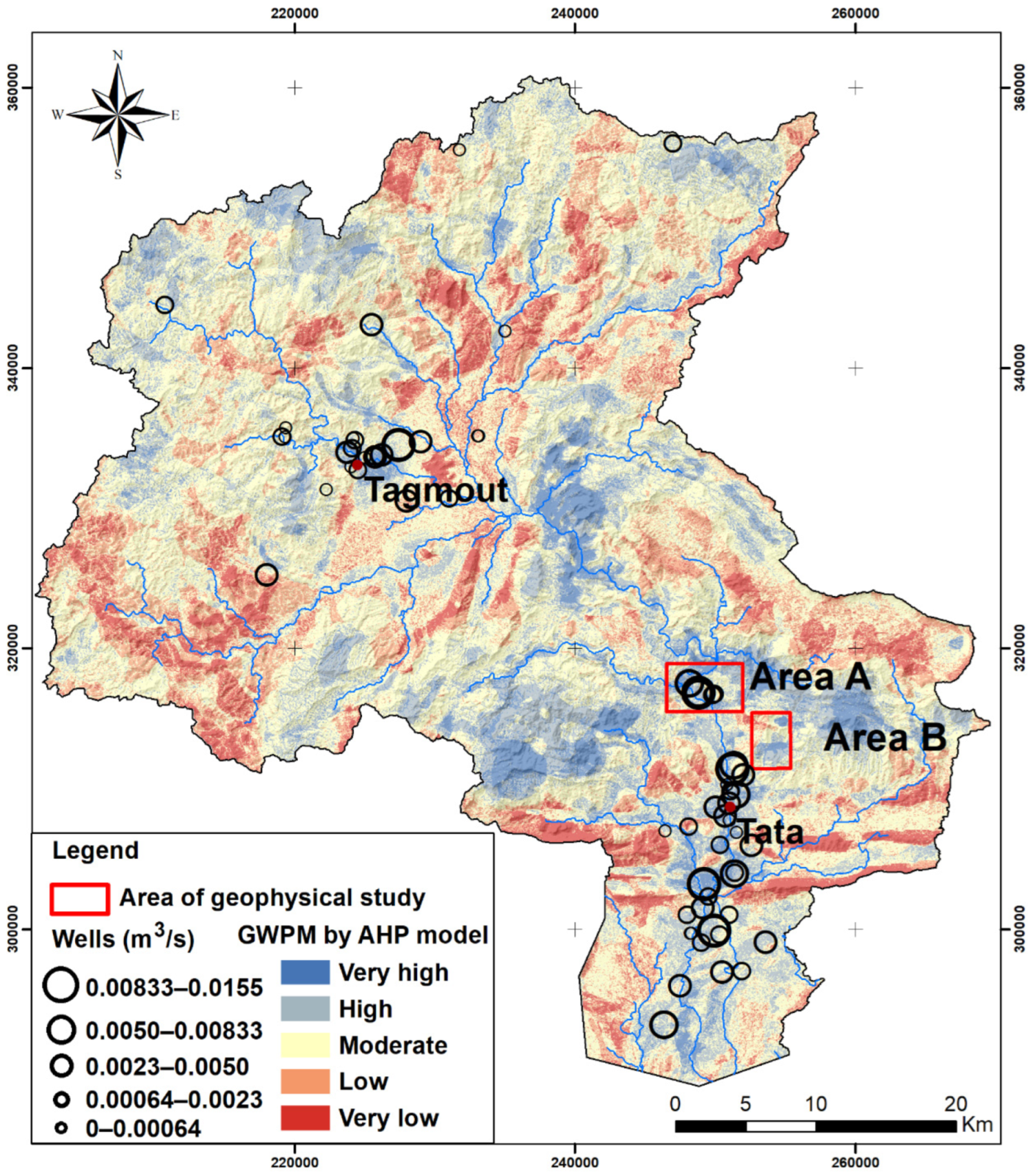
4.1. GWPMusing AHP Model
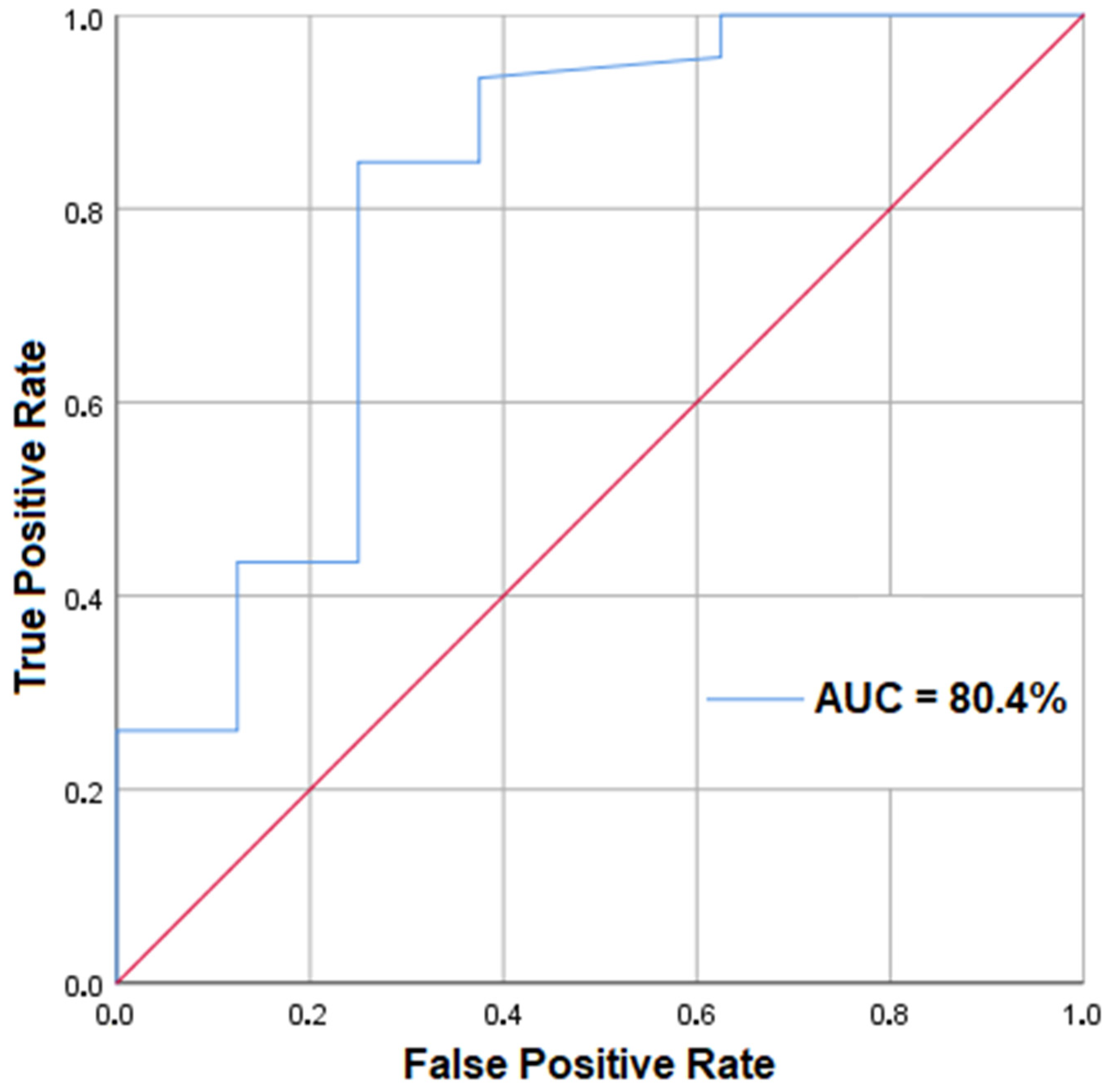
4.2. Validation of GWPM
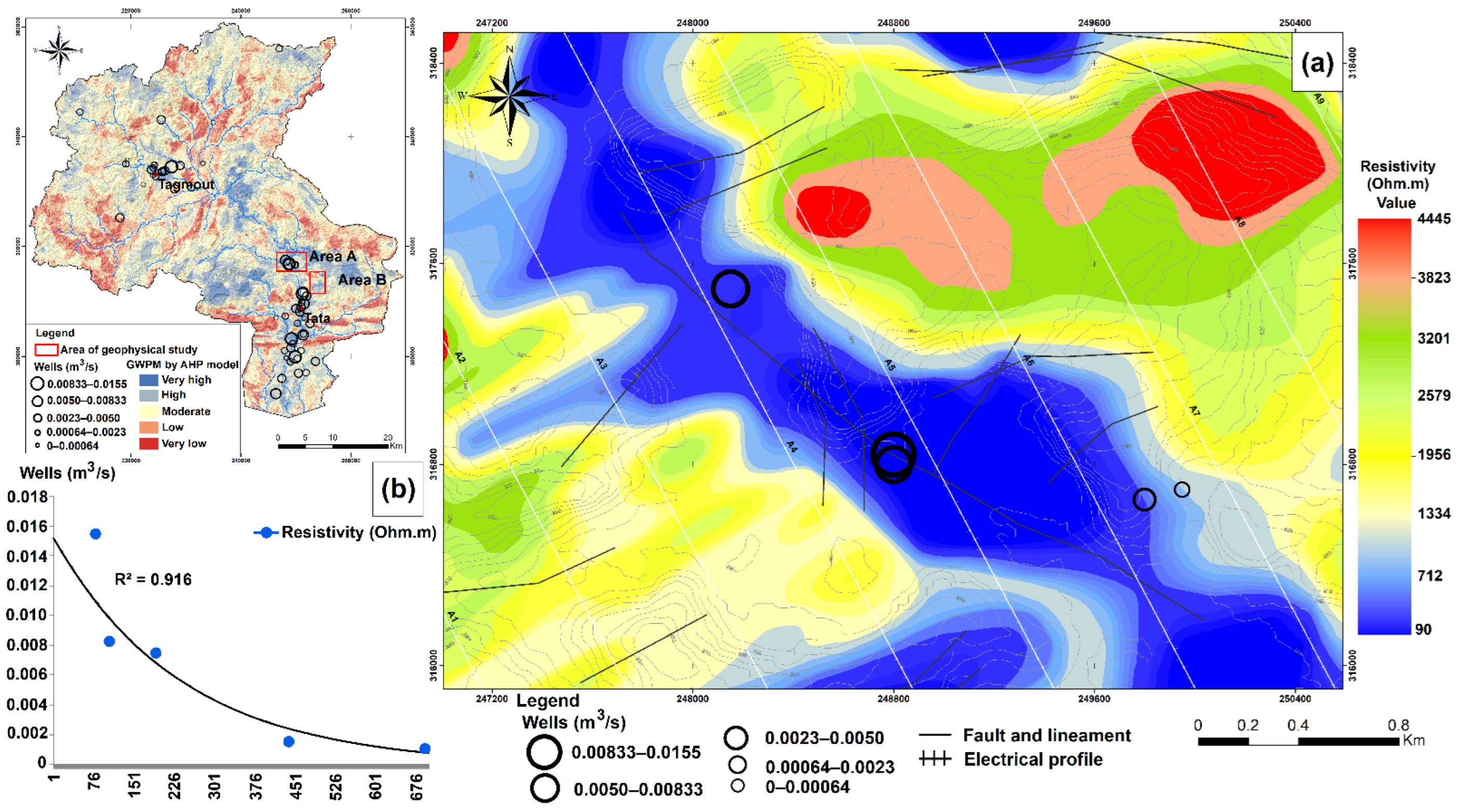
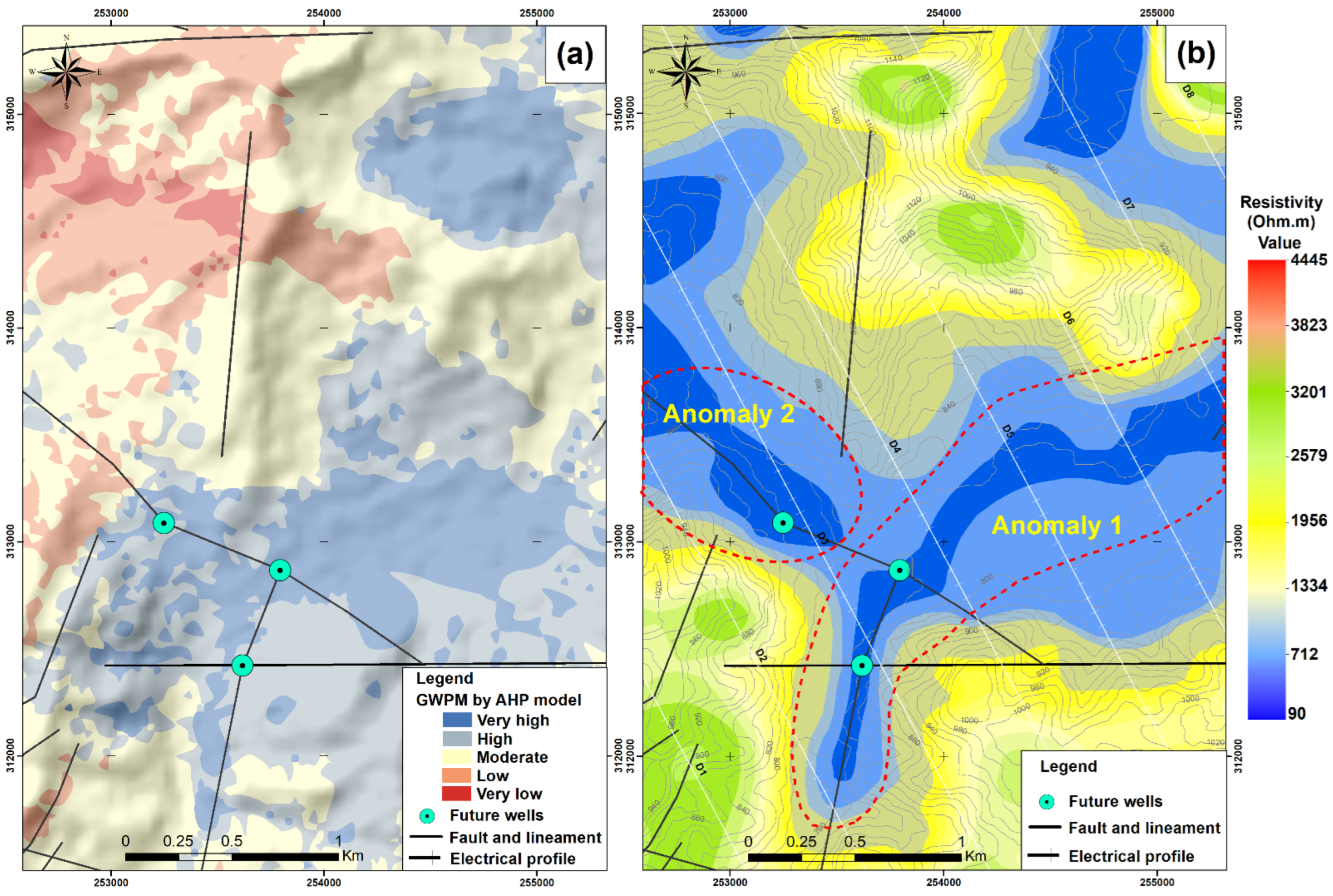
4.3. Application of Geophysics: Analysis and Interpretation of Results for Area A (NE of Tata City)
- Anomaly 1, which corresponds to the basement formations at a depth affected by faults and hydrogeological lineaments with an alluvial cover above and
- Anomaly 2, which corresponds to NW–SE faults affecting the limestone formations without alluvial cover.
5. Conclusions
Author Contributions
Funding
Data Availability Statement
Acknowledgments
Conflicts of Interest
Nomenclature
| AHP | Analytical hierarchy process |
| PER | Permeability |
| SL | Slope |
| ND | Node density |
| TWI | Topographic wetness index |
| STI | Stream transport index |
| SPI | Stream power index |
| PLC | Plan curvature |
| PRC | Profile curvature |
| DD | Drainage density |
| GIS | Geographic Information System |
| RS | Teledetection |
| GWPM | Groundwater potential map |
| ROC | Receiver operating characteristics |
| AUC | Area under the curve |
| DEM | Digital elevation model |
| FR | Frequency ratio |
| EBF | Evidential belief function |
| SE | Shannon’s entropy |
| BRT | Boosted regression tree |
| LR | Logistic regression |
| SI | Statistical index |
| CR | Consistency ratio |
| RI | Random index |
| CI | Consistency index |
References
- Pouffary, S.; De Laboulaye, G.; Antonini, A.; Quefelec, S.; Dittrick, L. Les Défis Du Changement Climatique En Méditerranée. Transformer Les Contraintes En Opportunités D’agir; ENERGIES 2050: Biot, France, 2016. [Google Scholar]
- DRPE. Etude D’actualisation Du Plan Directeur D’aménagement Intégré Des Ressources En Eau (PDAIRE) Du Bassin Hydraulique Du Draa; Secrétariat d’Etat auprès du Ministère de l’Energie, des Mines, de l’Eau et de l’Environnement, chargé de l’Eau et de l’Environnement: Rabat, Morocco, 2008.
- Echogdali, F.Z.; Boutaleb, S.; Jauregui, J.; Elmouden, A. Cartography of Flooding Hazard in Semi–Arid Climate: The Case of Tata Valley (South–East of Morocco). J. Geogr. Nat. Disast. 2018, 8, 214. [Google Scholar] [CrossRef]
- Panahi, M.; Sadhasivam, N.; Pourghasemi, H.R.; Rezaie, F.; Lee, S. Spatial prediction of groundwater potential mapping based on convolutional neural network (CNN) and support vector regression (SVR). J. Hydrol. 2020, 588, 125033. [Google Scholar] [CrossRef]
- Sander, P.; Minor, T.B.; Chesley, M.M. Ground-Water Exploration Based on Lineament Analysis and Reproducibility Tests. Groundwater 1997, 35, 888–894. [Google Scholar] [CrossRef]
- Israil, M.; Al-Hadithi, M.; Singhal, D.C. Application of a resistivity survey and geographical information system (GIS) analysis for hydrogeological zoning of a piedmont area, Himalayan foothill region, India. Appl. Hydrogeol. 2005, 14, 753–759. [Google Scholar] [CrossRef]
- Wieland, M.; Pittore, M. A Spatio-Temporal Building Exposure Database and Information Life-Cycle Management Solution. ISPRS Int. J. Geo-Inf. 2017, 6, 114. [Google Scholar] [CrossRef]
- Souissi, D.; Msaddek, M.H.; Zouhri, L.; Chenini, I.; El May, M.; Dlala, M. Mapping groundwater recharge potential zones in arid region using GIS and Landsat approaches, southeast Tunisia. Hydrol. Sci. J. 2018, 63, 251–268. [Google Scholar] [CrossRef]
- Ghosh, D.; Mandal, M.; Banerjee, M.; Karmakar, M. Impact of hydro-geological environment on availability of groundwater using analytical hierarchy process (AHP) and geospatial techniques: A study from the upper Kangsabati river basin. Groundw. Sustain. Dev. 2020, 11, 100419. [Google Scholar] [CrossRef]
- Khan, M.Y.A.; ElKashouty, M.; Tian, F. Mapping Groundwater Potential Zones Using Analytical Hierarchical Process and Multicriteria Evaluation in the Central Eastern Desert, Egypt. Water 2022, 14, 1041. [Google Scholar] [CrossRef]
- Hussein, A.-A.; Govindu, V.; Nigusse, A.G.M. Evaluation of groundwater potential using geospatial techniques. Appl. Water Sci. 2016, 7, 2447–2461. [Google Scholar] [CrossRef] [Green Version]
- Stafford, K.W.; Rosales-Lagarde, L.; Boston, P.J. Castile evaporite karst potential map of the Gypsum Plain, Eddy County, New Mexico and Culberson County, Texas: A GIS methodological comparison. J. Cave Karst Stud. 2008, 70, 35–46. [Google Scholar]
- Zghibi, A.; Mirchi, A.; Msaddek, M.H.; Merzougui, A.; Zouhri, L.; Taupin, J.-D.; Chekirbane, A.; Chenini, I.; Tarhouni, J. Using Analytical Hierarchy Process and Multi-Influencing Factors to Map Groundwater Recharge Zones in a Semi-arid Mediterranean Coastal Aquifer. Water 2020, 12, 2525. [Google Scholar] [CrossRef]
- Naghibi, S.A.; Pourghasemi, H.R.; Pourtaghi, Z.S.; Rezaei, A. Groundwater qanat potential mapping using frequency ratio and Shannon’s entropy models in the Moghan watershed, Iran. Earth Sci. Inform. 2014, 8, 171–186. [Google Scholar] [CrossRef]
- Regmi, A.D.; Devkota, K.C.; Yoshida, K.; Pradhan, B.; Pourghasemi, H.R.; Kumamoto, T.; Akgun, A. Application of frequency ratio, statistical index, and weights–of–evidence models and their comparison in landslide susceptibility mapping in Central Nepal Himalaya. Arab. J. Geosci. 2014, 7, 725–742. [Google Scholar] [CrossRef]
- Mogaji, K.A.; Lim, H.S.; Abdullah, K. Regional prediction of groundwater potential mapping in a multifaceted geology terrain using GIS-based Dempster–Shafer model. Arab. J. Geosci. 2014, 8, 3235–3258. [Google Scholar] [CrossRef]
- Naghibi, S.A.; Pourghasemi, H.R.; Dixon, B. GIS–based groundwater potential mapping using boosted regression tree, classification and regression tree, and random forest machine learning models in Iran. Environ. Monit. Assess. 2016, 188, 44. [Google Scholar] [CrossRef] [PubMed]
- Pourtaghi, Z.S.; Pourghasemi, H.R. GIS–based groundwater spring potential assessment and mapping in the Birjand Township, southern Khorasan Province. Iran. Hydrogeol. J. 2014, 22, 643–662. [Google Scholar] [CrossRef]
- Falah, F.; Nejad, S.G.; Rahmati, O.; Daneshfar, M.; Zeinivand, H. Applicability of generalized additive model in groundwater potential modelling and comparison its performance by bivariate statistical methods. Geocarto Int. 2016, 32, 1069–1089. [Google Scholar] [CrossRef]
- Shao, Z.; Huq, E.; Cai, B.; Altan, O.; Li, Y. Integrated remote sensing and GIS approach using Fuzzy-AHP to delineate and identify groundwater potential zones in semi-arid Shanxi Province, China. Environ. Model. Softw. 2020, 134, 104868. [Google Scholar] [CrossRef]
- Kumar, T.; Gautam, A.K.; Kumar, T. Appraising the accuracy of GIS–based multi–criteria decision making technique for delineation of groundwater potential zones. Water Resour. Manag. 2014, 28, 4449–4466. [Google Scholar] [CrossRef]
- Murmu, P.; Kumar, M.; Lal, D.; Sonker, I.; Singh, S.K. Delineation of groundwater potential zones using geospatial techniques and analytical hierarchy process in Dumka district, Jharkhand, India. Groundw. Sustain. Dev. 2019, 9, 100239. [Google Scholar] [CrossRef]
- Abijith, D.; Saravanan, S.; Singh, L.; Jennifer, J.J.; Saranya, T.; Parthasarathy, K. GIS-based multi-criteria analysis for identification of potential groundwater recharge zones—A case study from Ponnaniyaru watershed, Tamil Nadu, India. HydroResearch 2020, 3, 1–14. [Google Scholar] [CrossRef]
- Arefin, R. Groundwater potential zone identification at Plio-Pleistocene elevated tract, Bangladesh: AHP-GIS and remote sensing approach. Groundw. Sustain. Dev. 2020, 10, 100340. [Google Scholar] [CrossRef]
- Al-Ruzouq, R.; Shanableh, A.; Merabtene, T.; Siddique, M.; Khalil, M.A.; Idris, A.; Almulla, E. Potential groundwater zone mapping based on geo-hydrological considerations and multi-criteria spatial analysis: North UAE. CATENA 2018, 173, 511–524. [Google Scholar] [CrossRef]
- Jothibasu, A.; Anbazhagan, S. Modeling groundwater probability index in Ponnaiyar River basin of South India using analytic hierarchy process. Model. Earth Syst. Environ. 2016, 2, 109. [Google Scholar] [CrossRef] [Green Version]
- Echogdali, F.Z.; Boutaleb, S.; Taia, S.; Ouchchen, M.; Id–Belqas, M.; Kpan, R.B.; Abioui, M.; Aswathi, J.; Sajinkumar, K.S. Assessment of soil erosion risk in a semi–arid climate watershed using SWAT model: Case of Tata basin, South–East of Morocco. Appl. Water Sci. 2022, 12, 137. [Google Scholar] [CrossRef]
- Choubert, G. Histoire géologique du précambrien de l’Anti–Atlas. Notes Mem. Serv. Geol. Maroc 1963, 162, 352. [Google Scholar]
- Faik, F.; Belfoul, M.A.; Bouabdelli, M.; Hassenforder, B. Les structures de la couverture Néoprotérozoïque terminal et Paléozoïque de la région de Tata, Anti–Atlas centre–occidental, Maroc: Déformation polyphasée, ou interactions socle/couverture pendant l’orogenèse hercynienne? J. Afr. Earth Sci. 2001, 32, 765–776. [Google Scholar] [CrossRef]
- Algouti, A.; Algouti, A.; Chbani, B.; Zaim, M. Sédimentation et volcanisme synsédimentaire de la série de base de l’Adoudounien infra–cambrien à travers deux exemples de l’Anti–Atlas du Maroc. J. Afr. Earth Sci. 2001, 32, 541–556. [Google Scholar] [CrossRef]
- Benssaou, M.; Hamoumi, N. The western Anti-Atlas of Morocco: Sedimentological and palæogeographical formation studies in the Early Cambrian. J. Afr. Earth Sci. 2001, 32, 351–372. [Google Scholar] [CrossRef]
- Benssaou, M.; Hamoumi, N. Le graben de l’Anti–Atlas occidental (Maroc): Contrôle tectonique de la paléogéographie et des séquences au Cambrien inférieur. Comptes Rendus Geosci. 2003, 335, 297–305. [Google Scholar] [CrossRef]
- Ouchchen, M.; Boutaleb, S.; El Azzab, D.; Abioui, M.; Mickus, K.L.; Miftah, A.; Echogdali, F.Z.; Dadi, B. Structural interpretation of the Igherm region (Western Anti Atlas, Morocco) from an aeromagnetic analysis: Implications for copper exploration. J. Afr. Earth Sci. 2021, 176, 104140. [Google Scholar] [CrossRef]
- Echogdali, F.Z.; Boutaleb, S.; Abia, E.H.; Ouchchen, M.; Dadi, B.; Id-Belqas, M.; Abioui, M.; Pham, L.T.; Abu-Alam, T.; Mickus, K.L. Mineral prospectivity mapping: A potential technique for sustainable mineral exploration and mining activities—a case study using the copper deposits of the Tagmout basin, Morocco. Geocarto Int. 2021, 1–22. [Google Scholar] [CrossRef]
- Wendt, J. Disintegration of the continental margin of northwestern Gondwana: Late Devonian of the eastern Anti-Atlas (Morocco). Geology 1985, 13, 815. [Google Scholar] [CrossRef]
- Sahabi, M.; Aslanian, D.; Olivet, J.-L. Un nouveau point de départ pour l’histoire de l’Atlantique central. C. R. Geosci. 2004, 336, 1041–1052. [Google Scholar] [CrossRef] [Green Version]
- Ishizaka, A.; Labib, A. Review of the main developments in the analytic hierarchy process. Expert Syst. Appl. 2011, 38, 14336–14345. [Google Scholar] [CrossRef] [Green Version]
- Şener, Ş.; Sener, E.; Karagüzel, R. Solid waste disposal site selection with GIS and AHP methodology: A case study in Senirkent–Uluborlu (Isparta) Basin, Turkey. Environ. Monit Assess. 2011, 173, 533–554. [Google Scholar] [CrossRef]
- Pradhan, B. A comparative study on the predictive ability of the decision tree, support vector machine and neuro-fuzzy models in landslide susceptibility mapping using GIS. Comput. Geosci. 2013, 51, 350–365. [Google Scholar] [CrossRef]
- Chen, W.; Li, H.; Hou, E.; Wang, S.; Wang, G.; Panahi, M.; Li, T.; Peng, T.; Guo, C.; Niu, C.; et al. GIS–based groundwater potential analysis using novel ensemble weights–of–evidence with logistic regression and functional tree models. Sci. Total Environ. 2018, 634, 853–867. [Google Scholar] [CrossRef] [PubMed] [Green Version]
- Chowdhury, A.; Jha, M.K.; Chowdary, V.M.; Mal, B.C. Integrated remote sensing and GIS-based approach for assessing groundwater potential in West Medinipur district, West Bengal, India. Int. J. Remote Sens. 2009, 30, 231–250. [Google Scholar] [CrossRef]
- Laurent, F. Outils De Modélisation Spatiale Pour La Gestion Intégrée Des Ressources En Eau: Application Aux Schémas D’Aménagement Et De Gestion Des Eaux. Ph.D. Thesis, École Nationale Supérieure des Mines de Saint–Étienne/École Nationale Supérieure des Mines de Paris, Lyon, Paris, 1996. [Google Scholar]
- Khan, M.Y.A.; ElKashouty, M.; Subyani, A.M.; Tian, F.; Gusti, W. GIS and RS intelligence in delineating the groundwater potential zones in Arid Regions: A case study of southern Aseer, southwestern Saudi Arabia. Appl. Water Sci. 2021, 12, 3. [Google Scholar] [CrossRef]
- Bhattacharya, S.; Das, S.; Das, S.; Kalashetty, M.; Warghat, S.R. An integrated approach for mapping groundwater potential applying geospatial and MIF techniques in the semiarid region. Environ. Dev. Sustain. 2020, 23, 495–510. [Google Scholar] [CrossRef]
- Emran, A.; Chorowicz, J.; Cervelle, B.; Lyberis, N.; Tamain, G.; Alem, E.M. Cartographie géologique et analyse de la fracturation du sud de l’Anti–Atlas central (Maroc) à partir d’une image Landsat MSS. Photo Interprétation 1988, 27, 1–10. [Google Scholar]
- Boutaleb, S.; Boualoul, M.; Oudra, M.; Bouchaou, L.; Dindane, K. Apports du traitement d’image et de la géophysique à l’étude des ressources en eau en milieu fissuré: Cas de l’Anti–Atlas marocain. Afr. Geosci. Rev. 2008, 15, 129–141. [Google Scholar]
- Boutaleb, S.; Hammichi, F.; Tabyaoui, H.; Bouchaou, L.; Dindane, K. Détermination des écoulements préférentiels en zone karstique (Tafrata, Maroc), Apport des données satellitaires SAR ERS–1 et Landsat ETM+ et de la prospection géophysique. J. Water Sci. 2009, 22, 407–419. [Google Scholar]
- Chotin, P.; Ait Brahim, L.; Deffontaines, B.; Rudant, J.P.; Chaouni, A. Apports des données ERS1–SAR sur la reconnaissance du réseau de failles dans la péninsule de Tanger, Maroc. Photo Interprétation 1995, 33, 146–152. [Google Scholar]
- Bouchaou, L.; Boutaleb, S.; Boualoul, M.; Oudra, M. Application of remote-sensing and surface geophysics for groundwater prospecting in a hard rock terrain, Morocco. In Applied Groundwater Studies in Africa; CRC Press: London, UK, 2008; pp. 215–230. [Google Scholar] [CrossRef]
- Hssaisoune, M.; Boutaleb, S.; Bouchaou, L.; Benssaou, M.; Tagma, T. Use of remote sensing and electrical resistivity tomography to determine Tidsi spring recharge and underground drainage. Eur. Water 2017, 57, 429–434. [Google Scholar]
- Ozdemir, A. Using a binary logistic regression method and GIS for evaluating and mapping the groundwater spring potential in the Sultan Mountains (Aksehir, Turkey). J. Hydrol. 2011, 405, 123–136. [Google Scholar] [CrossRef]
- Selvam, S.; Magesh, N.S.; Sivasubramanian, P.; Soundranayagam, J.P.; Manimaran, G.; Seshunarayana, T. Deciphering of groundwater potential zones in Tuticorin, Tamil Nadu, using remote sensing and GIS techniques. J. Geol. Soc. India 2014, 84, 597–608. [Google Scholar] [CrossRef]
- Sharma, K.D.; Singh, H.P.; Pareek, O.P. Rainwater infiltration into a bare loamy sand. Hydrol. Sci. J. 1983, 28, 417–424. [Google Scholar] [CrossRef] [Green Version]
- Fox, D.; Bryan, R.; Price, A. The influence of slope angle on final infiltration rate for interrill conditions. Geoderma 1997, 80, 181–194. [Google Scholar] [CrossRef]
- Lee, S.; Kim, Y.-S.; Oh, H.-J. Application of a weights-of-evidence method and GIS to regional groundwater productivity potential mapping. J. Environ. Manag. 2012, 96, 91–105. [Google Scholar] [CrossRef] [PubMed]
- Moore, I.D.; Grayson, R.B.; Ladson, A.R. Digital terrain modelling: A review of hydrological, geomorphological, and biological applications. Hydrol. Process. 1991, 5, 3–30. [Google Scholar] [CrossRef]
- Kimerling, A.J.; Buckley, A.R.; Muehrcke, P.C.; Muehrcke, J.O. Map Use: Reading, Analysis, Interpretation, 8th ed.; ESRI Press Academic: Redlands, CA, USA, 2016. [Google Scholar]
- Oh, H.J.; Lee, S. Cross-validation of logistic regression model for landslide susceptibility mapping at Geneoung areas, Korea. Disaster Adv. 2010, 3, 44–55. [Google Scholar]
- Wischmeier, W.H.; Smith, D.D. Predicting Rainfall Erosion Losses: A Guide to Conservation Planning; United States Department of Agriculture: Washington, DC, USA, 1978.
- Moore, I.D.; Burch, G.J. Sediment Transport Capacity of Sheet and Rill Flow: Application of Unit Stream Power Theory. Water Resour. Res. 1986, 22, 1350–1360. [Google Scholar] [CrossRef]
- Rahmati, O.; Nazari Samani, A.; Mahdavi, M.; Pourghasemi, H.R.; Zeinivand, H. Groundwater potential mapping at Kurdistan region of Iran using analytic hierarchy process and GIS. Arab. J. Geosci. 2015, 8, 7059–7071. [Google Scholar] [CrossRef]
- Saranya, T.; Saravanan, S. Groundwater potential zone mapping using analytical hierarchy process (AHP) and GIS for Kancheepuram District, Tamilnadu, India. Model. Earth Syst. Environ. 2020, 6, 1105–1122. [Google Scholar] [CrossRef]
- Maity, D.K.; Mandal, S. Identification of groundwater potential zones of the Kumari river basin, India: An RS & GIS based semi-quantitative approach. Environ. Dev. Sustain. 2017, 21, 1013–1034. [Google Scholar] [CrossRef]
- Ikirri, M.; Faik, F.; Boutaleb, S.; Echogdali, F.Z.; Abioui, M.; Al-Ansari, N. Application of HEC-RAS/WMS and FHI models for extreme hydrological events under climate change in the Ifni River arid watershed from Morocco. In Climate and Land Use Impacts on Natural and Artificial Systems; Elsevier: Amsterdam, The Netherlands, 2021; pp. 251–270. [Google Scholar] [CrossRef]
- Echogdali, F.Z.; Boutaleb, S.; Elmouden, A.; Ouchchen, M. Assessing Flood Hazard at River Basin Scale: Comparison between HECRAS-WMS and Flood Hazard Index (FHI) Methods Applied to El Maleh Basin, Morocco. J. Water Resour. Prot. 2018, 10, 957–977. [Google Scholar] [CrossRef] [Green Version]
- Echogdali, F.Z.; Kpan, R.B.; Ouchchen, M.; Id-Belqas, M.; Dadi, B.; Ikirri, M.; Abioui, M.; Boutaleb, S. Spatial Prediction of Flood Frequency Analysis in a Semi-Arid Zone: A Case Study from the Seyad Basin (Guelmim Region, Morocco). In Geospatial Technology for Landscape and Environmental Management; Springer: Berlin, Germany, 2022; pp. 49–71. [Google Scholar] [CrossRef]
- Razandi, Y.; Pourghasemi, H.R.; Neisani, N.S.; Rahmati, O. Application of analytical hierarchy process, frequency ratio, and certainty factor models for groundwater potential mapping using GIS. Earth Sci. Inform. 2015, 8, 867–883. [Google Scholar] [CrossRef]
- Dar, T.; Rai, N.; Bhat, A. Delineation of potential groundwater recharge zones using analytical hierarchy process (AHP). Geol. Ecol. Landsc. 2020, 5, 292–307. [Google Scholar] [CrossRef] [Green Version]
- Saaty, T.L. A scaling method for priorities in hierarchical structures. J. Math. Psychol. 1977, 15, 234–281. [Google Scholar] [CrossRef]
- Saaty, T.L. How to make a decision: The analytic hierarchy process. Eur. J. Oper. Res. 1990, 48, 9–26. [Google Scholar] [CrossRef]
- Saaty, T.L. Decision making with the analytic hierarchy process. Int. J. Serv. Sci. 2008, 1, 83–98. [Google Scholar] [CrossRef] [Green Version]
- Sutradhar, S.; Mondal, P.; Das, N. Delineation of groundwater potential zones using MIF and AHP models: A micro–level study on Suri Sadar Sub–Division, Birbhum District, West Bengal, India. Groundw. Sustain. Dev. 2021, 12, 100547. [Google Scholar] [CrossRef]
- Saaty, T.L. The Analytic Hierarchy Process: Planning, Priority Setting, Resources Allocation; McGraw: New York, NY, USA, 1980. [Google Scholar] [CrossRef]
- Kumar, V.; Jain, K. Site suitability evaluation for urban development using remote sensing, GIS and analytic hierarchy process (AHP). In Proceedings of the International Conference on Computer Vision and Image Processing; Springer: Singapore, 2017; pp. 377–388. [Google Scholar] [CrossRef]
- Vellaikannu, A.; Palaniraj, U.; Karthikeyan, S.; Senapathi, V.; Viswanathan, P.M.; Sekar, S. Identification of groundwater potential zones using geospatial approach in Sivagangai district, South India. Arab. J. Geosci. 2021, 14, 8. [Google Scholar] [CrossRef]
- Rahmati, O.; Pourghasemi, H.R.; Melesse, A.M. Application of GIS-based data driven random forest and maximum entropy models for groundwater potential mapping: A case study at Mehran Region, Iran. CATENA 2016, 137, 360–372. [Google Scholar] [CrossRef]
- Pourghasemi, H.R.; Moradi, H.R.; Aghda, S.M.F. Landslide susceptibility mapping by binary logistic regression, analytical hierarchy process, and statistical index models and assessment of their performances. Nat. Hazards 2013, 69, 749–779. [Google Scholar] [CrossRef]
- Chen, W.; Peng, J.; Hong, H.; Shahabi, H.; Pradhan, B.; Liu, J.; Zhu, A.X.; Pei, X.; Duan, Z. Landslide susceptibility modelling using GIS–based machine learning techniques for Chongren County, Jiangxi Province, China. Sci. Total Environ. 2018, 626, 1121–1135. [Google Scholar] [CrossRef]
- Bui, D.T.; Pradhan, B.; Lofman, O.; Revhaug, I.; Dick, O.B. Landslide susceptibility mapping at Hoa Binh province (Vietnam) using an adaptive neuro-fuzzy inference system and GIS. Comput. Geosci. 2012, 45, 199–211. [Google Scholar] [CrossRef]
- Jaafari, A.; Najafi, A.; Pourghasemi, H.R.; Rezaeian, J.; Sattarian, A. GIS-based frequency ratio and index of entropy models for landslide susceptibility assessment in the Caspian forest, northern Iran. Int. J. Environ. Sci. Technol. 2014, 11, 909–926. [Google Scholar] [CrossRef] [Green Version]
- Yesilnacar, E.K. The Application of Computational Intelligence to Landslide Susceptibility Mapping in Turkey. Ph.D. Thesis, University of Melbourne, Melbourne, Australia, 2005. [Google Scholar]
- Benjmel, K.; Amraoui, F.; Boutaleb, S.; Ouchchen, M.; Tahiri, A.; Touab, A. Mapping of groundwater potential zones in crystalline terrain using remote sensing, GIS techniques, and multicriteria data analysis (Case of the Ighrem Region, Western Anti-Atlas, Morocco). Water 2020, 12, 471. [Google Scholar] [CrossRef] [Green Version]
- Pal, S.C.; Ghosh, C.; Chowdhuri, I. Assessment of groundwater potentiality using geospatial techniques in Purba Bardhaman district, West Bengal. Appl. Water Sci. 2020, 10, 221. [Google Scholar] [CrossRef]
- Das, B.; Pal, S.C. Assessment of groundwater vulnerability to over-exploitation using MCDA, AHP, fuzzy logic and novel ensemble models: A case study of Goghat-I and II blocks of West Bengal, India. Environ. Earth Sci. 2020, 79, 104. [Google Scholar] [CrossRef]
- Pathmanandakumar, V.; Thasarathan, N.; Ranagalage, M. An Approach to Delineate Potential Groundwater Zones in Kilinochchi District, Sri Lanka, Using GIS Techniques. ISPRS Int. J. Geo-Inf. 2021, 10, 730. [Google Scholar] [CrossRef]
- Kumar, V.A.; Mondal, N.C.; Ahmed, S. Identification of Groundwater Potential Zones Using RS, GIS and AHP Techniques: A Case Study in a Part of Deccan Volcanic Province (DVP), Maharashtra, India. J. Indian Soc. Remote Sens. 2020, 48, 497–511. [Google Scholar] [CrossRef]
- Al-Abadi, A.M. Modeling of groundwater productivity in northeastern Wasit Governorate, Iraq using frequency ratio and Shannon’s entropy models. Appl. Water Sci. 2015, 7, 699–716. [Google Scholar] [CrossRef] [Green Version]
- Akula, A.; Singh, A.; Ghosh, R.; Kumar, S.; Sardana, H.K. Target recognition in infrared imagery using convolutional neural network. In Proceedings of the International Conference on Computer Vision and Image Processing; Springer: Singapore, 2017; pp. 25–34. [Google Scholar] [CrossRef]
- Mohammadzadeh, A.; Zoej, M.J.V.; Tavakoli, A. Automatic main road extraction from high resolution satellite imageries by means of particle swarm optimization applied to a fuzzy-based mean calculation approach. J. Indian Soc. Remote Sens. 2009, 37, 173–184. [Google Scholar] [CrossRef]
- Benjmel, K.; Amraoui, F.; Aydda, A.; Tahiri, A.; Yousif, M.; Pradhan, B.; Abdelrahman, K.; Fnais, M.S.; Abioui, M. A multidisciplinary approach for groundwater potential mapping in a fractured semi-arid terrain (Kerdous Inlier, Western Anti-Atlas, Morocco). Water 2022, 14, 1553. [Google Scholar] [CrossRef]
- Aswathi, J.; Sajinkumar, K.; Rajaneesh, A.; Oommen, T.; Bouali, E.; Binojkumar, R.; Rani, V.; Thomas, J.; Thrivikramji, K.; Ajin, R.; et al. Furthering the precision of RUSLE soil erosion with PSInSAR data: An innovative model. Geocarto Int. 2022, 1–22. [Google Scholar] [CrossRef]


| Factor (units) | Class | Rating | Weight | Factor (units) | Class | Rating | Weight |
|---|---|---|---|---|---|---|---|
| Drainage density (m/km2) | 1.56–1.85 | 1 | 1.85 | TWI | 5.68–8.78 | 1 | 0.55 |
| 1.25–1.56 | 3 | 8.78–10.42 | 3 | ||||
| 0.84–1.25 | 5 | 10.42–12.69 | 5 | ||||
| 0.59–0.84 | 8 | 12.69–16.28 | 8 | ||||
| 0.33–0.59 | 10 | 16.28–26.47 | 10 | ||||
| Node density (m/km2) | 0–0.21 | 1 | 1.86 | STI | 1568–3702 | 1 | 0.64 |
| 0.21–0.49 | 3 | 726–1568 | 3 | ||||
| 0.49–0.82 | 5 | 275–726 | 5 | ||||
| 0.82–1.15 | 8 | 58–275 | 8 | ||||
| 1.15–2.04 | 10 | 0–58 | 10 | ||||
| Lineament density (m/km2) | 0–0.32 | 1 | 1.35 | SPI | 509,811–1,108,331 | 1 | 0.53 |
| 0.32–0.64 | 3 | 295,555–509,811 | 3 | ||||
| 0.64–0.97 | 5 | 5998–295,555 | 5 | ||||
| 0.97–1.37 | 8 | 160–5998 | 8 | ||||
| 1.37–2.19 | 10 | 0–160 | 10 | ||||
| Permeability | Low permeability | 1 | 1.27 | Plan curvature | 0.42–17.87 | 1 | 0.49 |
| Medium permeability | 3 | −0.55–−0.42 | 3 | ||||
| High permeability | 8 | −13.46–−0.55 | 5 | ||||
| Slope (%) | 16< | 1 | 0.96 | Profile curvature | –16.98–−0.69 | 1 | 0.49 |
| 12–16 | 3 | –0.69–0.44 | 3 | ||||
| 8–12 | 5 | −0.44–−15.21 | 5 | ||||
| 4–8 | 8 | ||||||
| 0–4 | 10 |
| Factor | DD | ND | LD | PER | SL | TWI | STI | SPI | PLC | PRC |
|---|---|---|---|---|---|---|---|---|---|---|
| DD | 1 | 2 | 1 | 3 | 2 | 3 | 3 | 2 | 3 | 3 |
| ND | 1/2 | 1 | 4 | 1 | 2 | 2 | 4 | 4 | 4 | 4 |
| LD | 1 | 1/4 | 1 | 1/2 | 3 | 2 | 3 | 3 | 3 | 3 |
| PER | 1/3 | 1 | 2 | 1 | 2 | 3 | 2 | 2 | 2 | 2 |
| SL | 1/2 | 1/2 | 1/3 | 1/2 | 1 | 4 | 2 | 2 | 2 | 2 |
| TWI | 1/3 | 1/2 | 1/2 | 1/3 | 1/4 | 1 | 1/2 | 1/2 | 2 | 2 |
| STI | 1/3 | 1/4 | 1/3 | 1/2 | 1/2 | 2 | 1 | 1 | 2 | 2 |
| SPI | 1/2 | 1/4 | 1/3 | 1/2 | 1/2 | 2 | 1 | 1 | 1/2 | 1/2 |
| PLC | 1/3 | 1/4 | 1/3 | 1/2 | 1/2 | 1/2 | 1/2 | 2 | 1 | 1 |
| PRC | 1/3 | 1/4 | 1/3 | 1/2 | 1/2 | 1/2 | 1/2 | 2 | 1 | 1 |
| Factor | DD | ND | LD | PER | SL | TWI | STI | SPI | PLC | PRC | Weight |
|---|---|---|---|---|---|---|---|---|---|---|---|
| DD | 0.19 | 0.32 | 0.10 | 0.36 | 0.16 | 0.15 | 0.17 | 0.10 | 0.15 | 0.15 | 1.85 |
| ND | 0.10 | 0.16 | 0.39 | 0.12 | 0.16 | 0.10 | 0.23 | 0.21 | 0.20 | 0.20 | 1.86 |
| LD | 0.19 | 0.04 | 0.10 | 0.06 | 0.24 | 0.10 | 0.17 | 0.15 | 0.15 | 0.15 | 1.35 |
| PER | 0.06 | 0.16 | 0.20 | 0.12 | 0.16 | 0.15 | 0.11 | 0.10 | 0.10 | 0.10 | 1.27 |
| SL | 0.10 | 0.08 | 0.03 | 0.06 | 0.08 | 0.20 | 0.11 | 0.10 | 0.10 | 0.10 | 0.96 |
| TWI | 0.06 | 0.08 | 0.05 | 0.04 | 0.02 | 0.05 | 0.03 | 0.03 | 0.10 | 0.10 | 0.55 |
| STI | 0.06 | 0.04 | 0.03 | 0.06 | 0.04 | 0.10 | 0.06 | 0.05 | 0.10 | 0.10 | 0.64 |
| SPI | 0.10 | 0.04 | 0.03 | 0.06 | 0.04 | 0.10 | 0.06 | 0.05 | 0.02 | 0.02 | 0.53 |
| PLC | 0.06 | 0.04 | 0.03 | 0.06 | 0.04 | 0.03 | 0.03 | 0.10 | 0.05 | 0.05 | 0.49 |
| PRC | 0.06 | 0.04 | 0.03 | 0.06 | 0.04 | 0.03 | 0.03 | 0.10 | 0.05 | 0.05 | 0.49 |
| n | 1 | 2 | 3 | 4 | 5 | 6 | 7 | 8 | 9 | 10 |
|---|---|---|---|---|---|---|---|---|---|---|
| RI | 0 | 0 | 0.58 | 0.9 | 1.12 | 1.24 | 1.32 | 1.41 | 1.45 | 1.49 |
Publisher’s Note: MDPI stays neutral with regard to jurisdictional claims in published maps and institutional affiliations. |
© 2022 by the authors. Licensee MDPI, Basel, Switzerland. This article is an open access article distributed under the terms and conditions of the Creative Commons Attribution (CC BY) license (https://creativecommons.org/licenses/by/4.0/).
Share and Cite
Echogdali, F.Z.; Boutaleb, S.; Bendarma, A.; Saidi, M.E.; Aadraoui, M.; Abioui, M.; Ouchchen, M.; Abdelrahman, K.; Fnais, M.S.; Sajinkumar, K.S. Application of Analytical Hierarchy Process and Geophysical Method for Groundwater Potential Mapping in the Tata Basin, Morocco. Water 2022, 14, 2393. https://doi.org/10.3390/w14152393
Echogdali FZ, Boutaleb S, Bendarma A, Saidi ME, Aadraoui M, Abioui M, Ouchchen M, Abdelrahman K, Fnais MS, Sajinkumar KS. Application of Analytical Hierarchy Process and Geophysical Method for Groundwater Potential Mapping in the Tata Basin, Morocco. Water. 2022; 14(15):2393. https://doi.org/10.3390/w14152393
Chicago/Turabian StyleEchogdali, Fatima Zahra, Said Boutaleb, Amine Bendarma, Mohamed Elmehdi Saidi, Mohamed Aadraoui, Mohamed Abioui, Mohammed Ouchchen, Kamal Abdelrahman, Mohammed S. Fnais, and Kochappi Sathyan Sajinkumar. 2022. "Application of Analytical Hierarchy Process and Geophysical Method for Groundwater Potential Mapping in the Tata Basin, Morocco" Water 14, no. 15: 2393. https://doi.org/10.3390/w14152393