
A River Channel Extraction Method Based on a Digital Elevation Model Retrieved from Satellite Imagery


1
College of Resource Environment and Tourism, Capital Normal University, Beijing 100048, China
2
State Key Laboratory of Simulation and Regulation of Water Cycle River Basin, China Institute of Water Resources and Hydropower, Beijing 100038, China
*
Authors to whom correspondence should be addressed.
Water 2022, 14(15), 2387; https://doi.org/10.3390/w14152387
Submission received: 31 May 2022
/
Revised: 28 June 2022
/
Accepted: 29 July 2022
/
Published: 1 August 2022
(This article belongs to the Special Issue High-Resolution Monitoring and Modelling for Water Resources Management: New Sensors, New Approaches and Applications)
Abstract
:The river border positioning is an important part of river surveys, which is crucial for water conservation project development, water resource use, water disasters, river regime monitoring, and many other applications related to water resources. Currently, satellite images or field measurements are used to extract river channels. However, satellite images are insufficiently precise, and field measurement requires significant manpower and cost. In this paper, a new method for river channel extraction is proposed, which is based on the combination of Jenks natural breaks classification method and digital elevation model (DEM), and then the river channel range is complemented by using the water range monitored by GF-1(Gaofen-1 satellite) in flood season. The overall precision is greater than 85%, and the Kappa values achieve moderate stability (0.41–0.60). Using this method, the extraction of river range is practicable and achievable, and the higher the DEM resolution, the better the extraction result.
1. Introduction
The path that a river follows is called its river course, which is usually a passable waterway [1]. The river channel border can be determined based on the properties of the river and its terrain. Determining the precise location of the boundary of the river channel is an important component of a river survey, as it aids to assess and monitor flood disasters. It also helps develop water conservation projects, appropriate utilization of water resources, and monitor river regime.
Field measurement and remote sensing are the two of the most common approaches for determining river channel ranges. Field measurement is precise; however, it is expensive in terms of human and material resources, as well as low measuring efficiency and speed. Remote sensing method has been widely used owing to its high efficiency and quick monitoring. Although remote sensing images can be used to quickly extract river channel ranges, the majority of the findings are inaccurate due to the influence of resolution and cloud cover. Wu et al. [2] proposed an algorithm for river boundary extraction of high-resolution images based on active contour model. Guneralp et al. [3] studied the demarcation of river flow boundary based on remote sensing image by using support vector machine (SVM) and image-derived auxiliary data layer, and the auxiliary data layer generated by edge detector and spatial domain texture statistics improved the accuracy of boundary division. Milad et al. [4] carried out mixed decomposition and super-resolution mapping (SRM) based on WorldView-3 and GeoEye images respectively, and estimated and spatially allocated water components in the mixed pixels respectively, improving the accuracy of river region classification.
All of these methods are for water boundary extraction. Water extraction based on river image in flood season can also be approximated as the range of river. However, the normalized water index (NDWI) method based on high-resolution satellite images is mostly used for water extraction [5]. Database segmentation is required to use NDWI to distinguish the water from vegetation, exposed land, construction land, etc., [6]. The largest intermodal difference (OTSU) algorithm has a simple and fast advantage, making its application in water split very broad. Yuan et al. [7] used OTSU to automatically calculate the threshold for NDWI to distinguish between water and non-water, and extracted the initial water information, followed by the local water and its background through the form, and calculated the local adaptive threshold, which not only realized the extraction of water information with adaptive threshold, but also improved the accuracy of water extraction. However, these methods are for the extraction of water boundary; water boundary cannot completely replace the range of river, generally smaller than the real range of river; therefore, the extraction accuracy is not enough.
Many researchers have used image analysis to extract riparian lines in order to better segment and identify river boundaries. Guo et al. [8] realized the vector description of river central skeleton and riverbank line in remote sensing images based on the aerial images of Yellow River, combined with PL (PolyGONAL LINE algorithm) and BP (back Propagation algorithm). In contrast to multispectral data, radar data are not affected by cloud cover. Zhu et al. [9] used the joint gray threshold segmentation and contour shape recognition method to extract the river channel from the remote sensing image obtained by the synthetic aperture radar (SAR) using the multi-level segmentation strategy, which can better extract the river channel region contour, and the dismissal alarm probability and false probability are low. Li et al. (2021) [10] proposed a new river extraction deep neural network model, River-Net, based on the high-precision extraction of river boundaries in synthetic aperture radar (SAR) images by combining the refined Lee filtering idea and the filtering characteristics of convolution operation. The results show that the proposed model can extract the river more accurately in SAR images than the mainstream semantic segmentation model.
Digital elevation model (DEM) is one of the most basic data sources for topographic relief information and watershed demarcation, and has been widely used in many hydrological studies [11]. The topographic elevation information contained in DEM can extract a large amount of surface morphological information, such as slope, aspect, and flow direction of watershed cells, etc. DEM is mainly used to extract drainage characteristics of watershed [12,13,14,15]. WU et al. [16] made an example application based on the principles and methods of water system and hydrology extraction, and improved the accuracy of the water system extraction. In addition to the extraction of water system, DEM data can also realize the division of watershed boundaries. Colombo R. et al. [17] used medium resolution (250 m) DEM to depict river networks and watershed boundaries across continental Europe, developed a new algorithm based on mathematical morphology, and realized landscape stratification of watershed density. The higher the resolution of DEM contains more information, the more accurate the extracted terrain information, and more widely used. Dong et al. [18] used local minimum search for water system identification, and used Bresenham’s line algorithm and mathematical morphology operation to divide the river. Muthusamy et al. [19] used different resolution DEMs to simulate the simulation of urban river floods. The river has special topographic undulation—the cross section of the river is mostly parabolic or trapezoid—so we can use the topographic trend of the river to find the appropriate extraction method to extract the range of the river. This requires an algorithm that can group and classify DEM and cluster and segment river range.
Jenks natural breaks classification method is a data clustering method proposed by Jenks [20]. Jenks natural breaks classification method in geographic information is mostly used to make thematic maps in ArcGIS software, and it is less used in geographic information research. The significance of Jenks natural breaks classification method is that the creator believes that there are some natural (non-human) turning points and breakpoints between any sequence. These natural breakpoints are statistically significant. Using these turning points, the research objects can be divided into groups with similar properties. Therefore, the natural breakpoint itself is a good boundary for classification [21]. The information contained in remote sensing data also has some natural turning points and breakpoints, which can be classified by Jenks natural breaks classification method. Chen et al. [22] with regard to the Jenks method and other methods, experimental studies in China’s surrounding geographic environment units, demonstrated that Jenks method divided into geographical environment unit has better adaptability and higher precision. DEM data contain elevation data of different places. If a natural intermittent classification algorithm is used in DEM, different elevated substances can also make natural packets in accordance with the specified number of categories, and the river is moving toward natural groups. The smallest packet of medium elevation.
This research investigated river range extraction based on digital elevation model (DEM) data and GF-1 data in order to extract river range reliably and fast, and suggested a new approach of river range extraction by combining Jenks natural breaks classification with digital elevation model.
The “natural discontinuity point” approach was used to build the “DEM channel extraction” model tool based on the usual “multi-crest feature” of the DEM histogram. The tool can extract channel ranges based on DEMs, and GF data are utilized as supplementary data, which eliminate the inaccuracy of channel extraction caused by the cloud resolution of multi-spectral images, and provides a foundation for further study of channel water regime.
2. Research Methods and Data Sources
2.1. Study Area
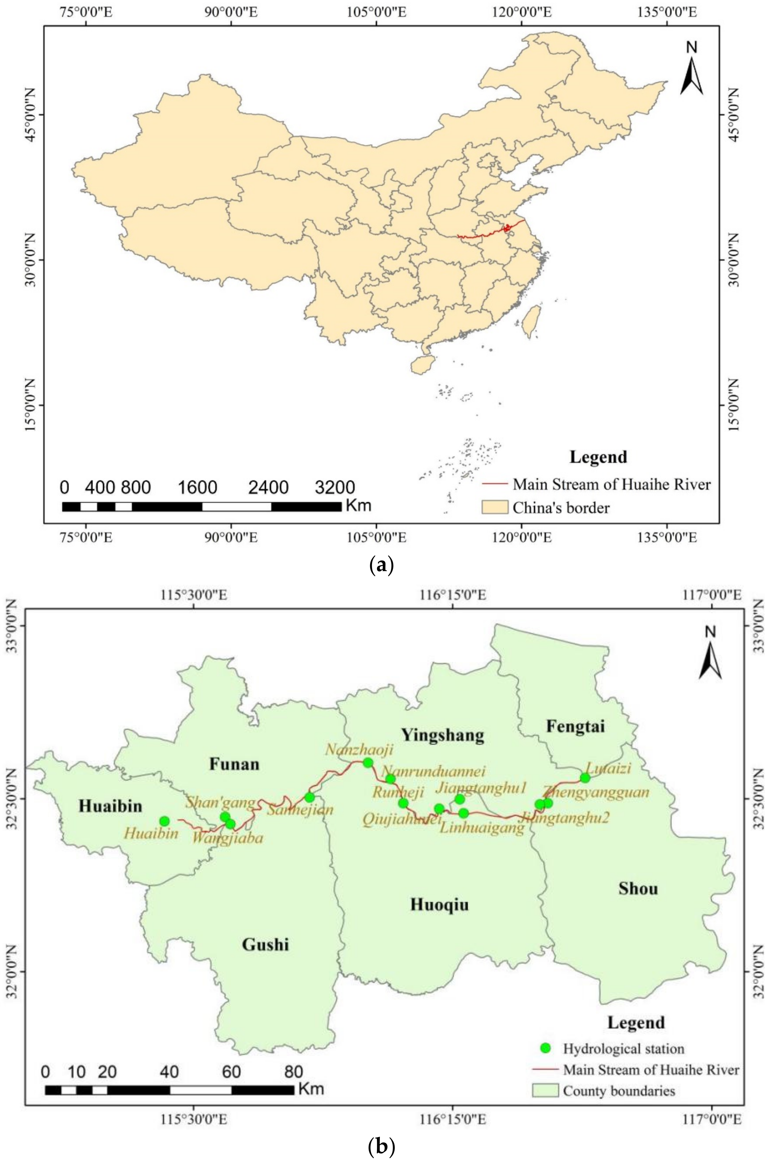
The main stream of Huaihe River from Huaibin station to Lutaizi station is selected as the study area. This part of the river flows through four cities and seven counties (Figure 1): Huaibin County (Xinyang City), Funan County (Fuyang City), Gushi County (Xinyang City), Yingshang County (Fuyang City), Huoqiu County (Lu’an City), Fengtai County (Huainan City), and Shou county (Huainan City). The total length is approximately 182.20 km. The study area is located in the Jianghuai Plain. There are many rivers and lakes in the plain, and the water system is developed. The overall terrain is high in the west and low in the east, but there is little difference in elevation. DEM in this region is also high in the west and low in the east with little fluctuation.
2.2. Research Route and Methods
2.2.1. Research Route
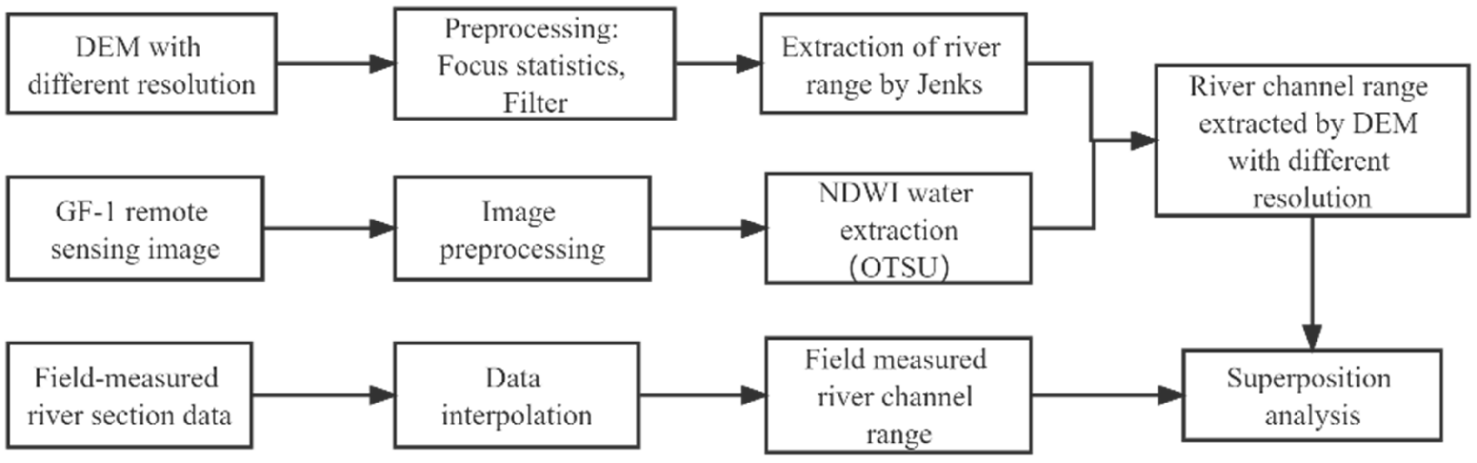
The research route of this study is shown in Figure 2. The statistics that were to be focused on and DEM filtering with different resolutions were preprocessed to adjust the contrast relationship between the grid pixel and its adjacent pixels to enhance the features of the ground objects. Then, the river channel was extracted by the natural discontinuity method to obtain the preliminary results of river channel range. For high-resolution images, NDWI water body was extracted, and OTSU was used to perform threshold segmentation to obtain water body range, which was used to complement the discontinuities of DEM extraction results in order to obtain river channel extraction range based on DEM with varying resolutions. The actual river range can be easily obtained from the measured section data, which can be used to verify the accuracy of the results. Overall accuracy (OA) and Kappa coefficient were used to verify the accuracy of the extraction results.
2.2.2. Methods
Jenks Natural Breaks Classification (Jenks) Method
George Frederick Jenks proposed the Jenks natural breaks classification method for data clustering [20]. It is a data classification method based on the natural grouping inherent in data. It seeks to minimize the average deviation of each class from the mean of the class and maximize the deviation of each class from the mean of other groups. That is, it seeks to reduce the variance within classes and maximize the variance between classes to determine the best arrangement of values in different classes [20,21]. The goodness of variance fit (GVF) is obtained by dividing the difference between the square deviation of array mean (SDAM) and the square deviation of class mean (SDCM) by SDAM:
X = array average; Z = average value of class.
The closer GVF is to 1, the better the effect is. The value of GVF can only be 1 when the intra-class change is 0.
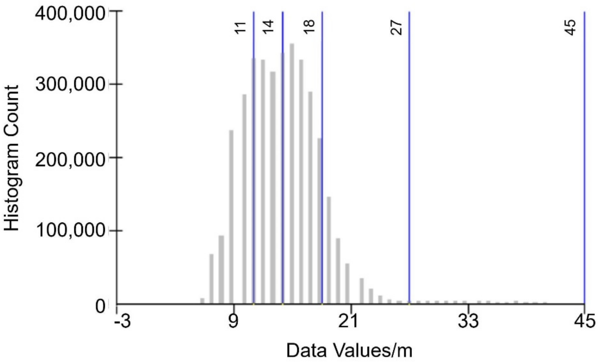
The histogram of DEM terrain has a typical feature of “multi-wave peak,” in which each “wave peak” represents a typical ground object, as shown in Figure 3. The river channel classification of this model adopts “natural discontinuity point” algorithm. The features with different elevations are naturally grouped according to the designated classification number, while the river and channel groups are the ones with the smallest elevation among the natural groups. The number of feature features is designated according to the number of feature features in DEM, which are reflected in different areas in DEM histogram, generally ranging from 3 to 10.
NDWI
McFeeters [23] introduced the normalized differential water index (NDWI) as a new data analysis method for water resource evaluation, which is used to describe the characteristics of open water and enhance the presence of open water in remote sensing digital images. NDWI uses near-infrared radiation and visible light to enhance the presence of water features while eliminating the influence of soil and terrestrial vegetation features.
The NDWI calculation formula is as follows:
where GREEN is the reflectivity of the green light band and NIR is the reflectivity of near-infrared band.
OTSU
The OTSU is a self-adaptive threshold determination method developed by a Japanese scholar Otsu [24], which is considered to be the optimal method for automatically selecting the threshold [24,25]. The method is derived from the least squares principle based on the gradation histogram, and has a statistical optimal segmentation threshold. Essentially, the grayscale histogram of the image with an optimal threshold is divided into two parts, in a manner such that the two parts are differential, meaning the maximum separation, the slumber is the smallest [26,27,28].
The image is separated into two types C1 (<TH) and C2 (>TH) by a threshold TH, the average value of the two types of pixels is M1 and M2, and the image global average is mG; the pixel is divided into C1 and C2. The C2 class has p1 and p2 probabilities, which follow the equations:
According to the concept of variance, the inter class variance is:
Equation (5) when subjected to Equation (7) can be simplified as:
where:
Using the ergodic method, the gray level K maximized by σ2 is the OTSU threshold.
Accuracy Verification Method
The accuracy verification used in this paper is: overall accuracy (OA) and Kappa coefficient:
(1) Overall accuracy:
OA is the simplest measure in remote sensing image classification and marks the proportion of correct pixels with respect to the total number of pixels. The larger the value, the better is the matching between the classification result; moreover, the higher the truth value the higher is the accuracy.
(2) Kappa
The Kappa coefficient is a common statistic of ground object classification and an indicator representing the correlation between classification results and truth values. The calculation method is as follows:
where, P0 is the number of all correctly classified pixels divided by the total number of samples, i.e., the OA. Pe is the product of the number of real pixels and the total number of classified pixels in the class divided by the total number of samples. The results of Kappa calculation are usually between 0 and 1, and can be divided into five categories to represent the degree of consistency at different levels, with 0–0.2 indicating very low consistency, 0.21–0.4 indicating general consistency, 0.41–0.60 indicating medium consistency, 0.61–0.80 indicating high consistency, and 0.81–1 indicating almost complete consistency.
2.3. Data Source
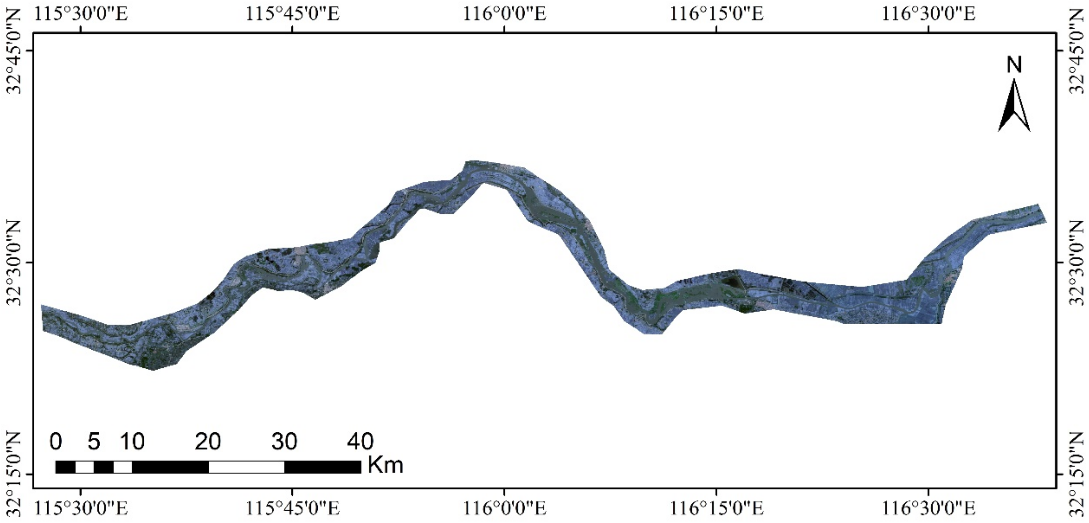
A variety of resolution DEM data were used in this study with resolutions of 30, 12.5, 5, and 2 m; for remote sensing data, we used GF-1 WFV optical multispectral image, from China Centre for Resources Satellite Data and Application (http://www.cresda.com/cn/, (accessed on 17 March 2022)). Among them, the high-score-first satellite is the first star in the national high-resolution to the ground observation system, which is equipped with two 2 m resolution full color (8 m) multispectral cameras and four 16 m resolution multispectral cameras. Data specific information is shown in Table 1, and the remote sensing data used is shown in Figure 3, Figure 4 and Figure 5 (the area of remote sensing data is 571.3 km2).
3. Results
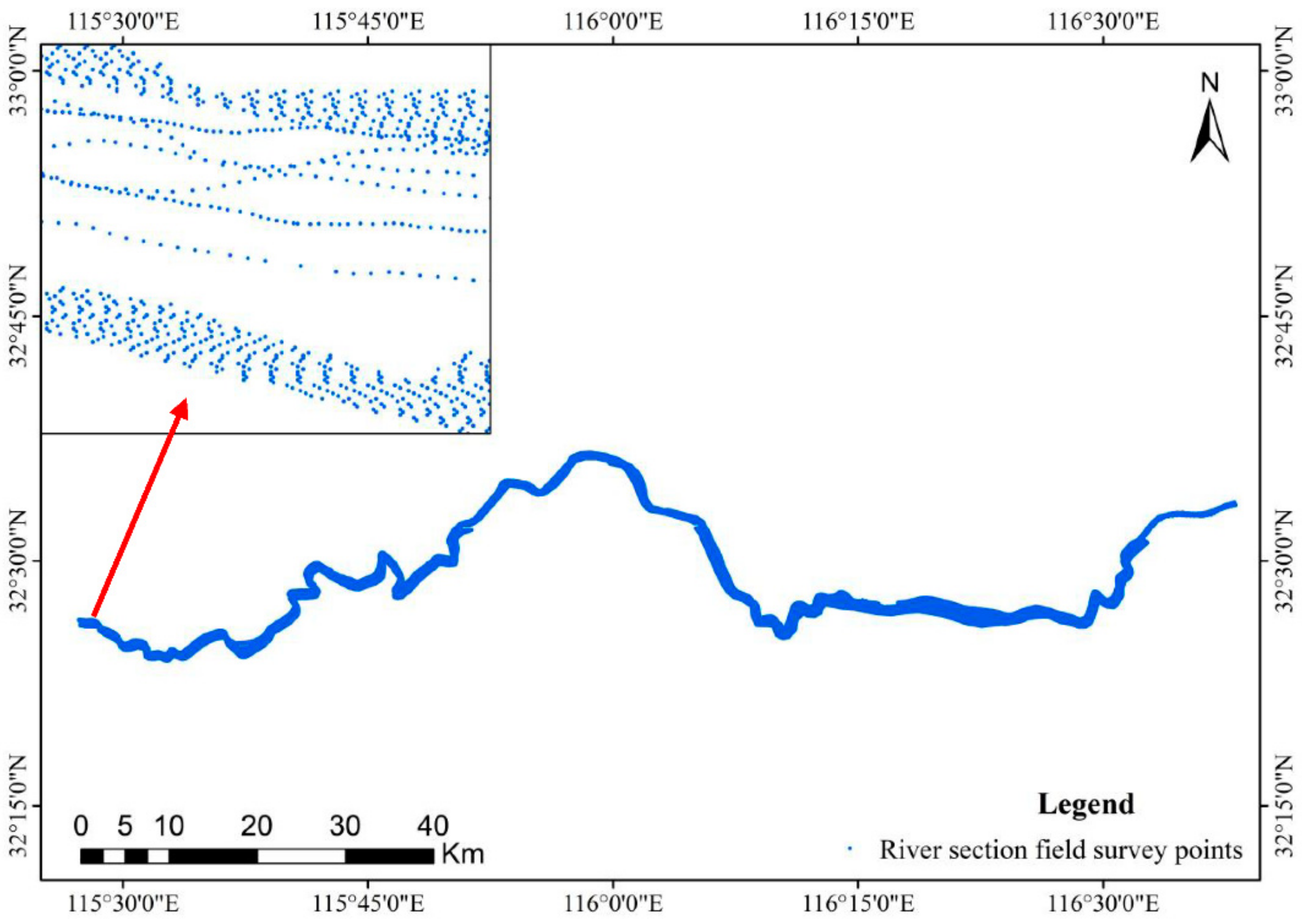
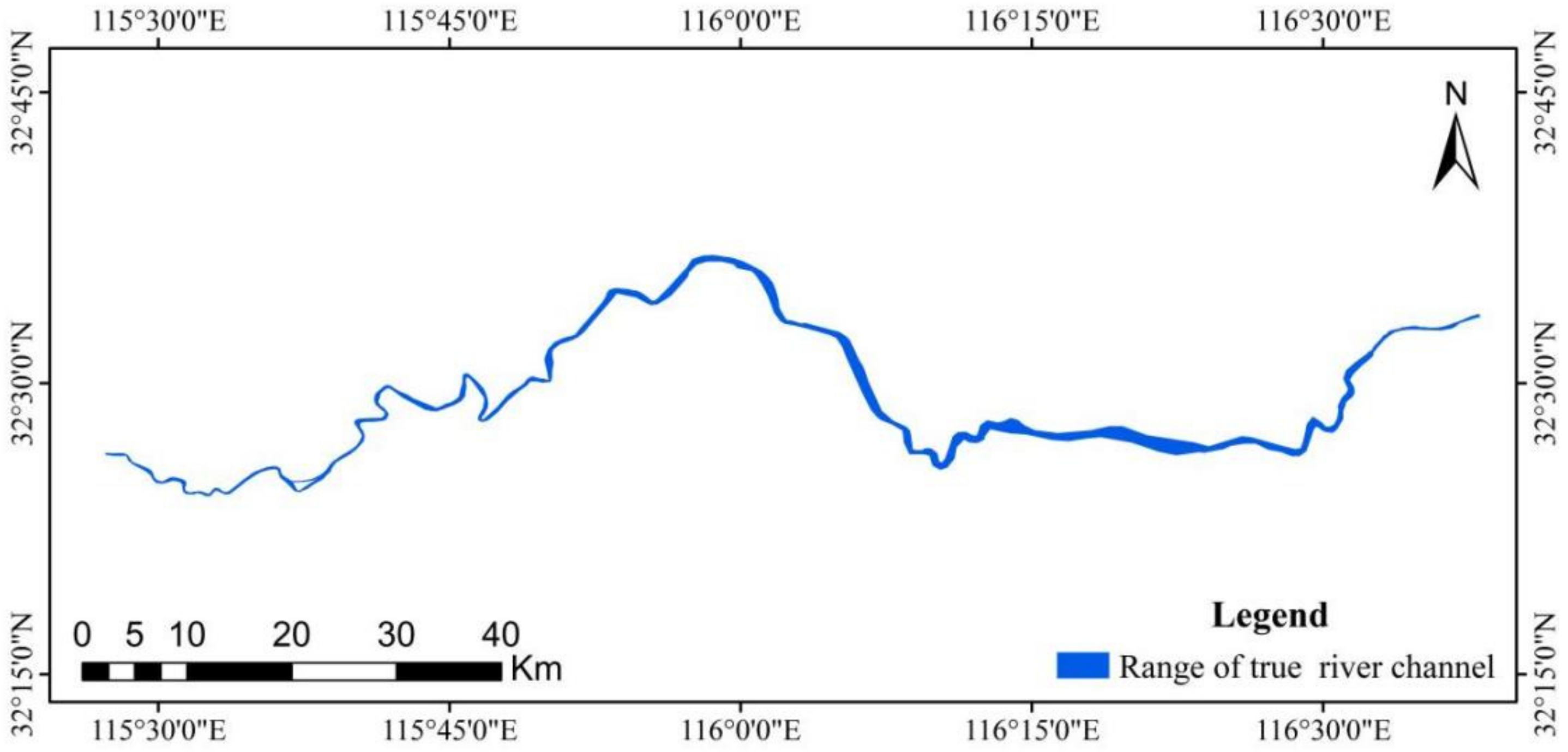
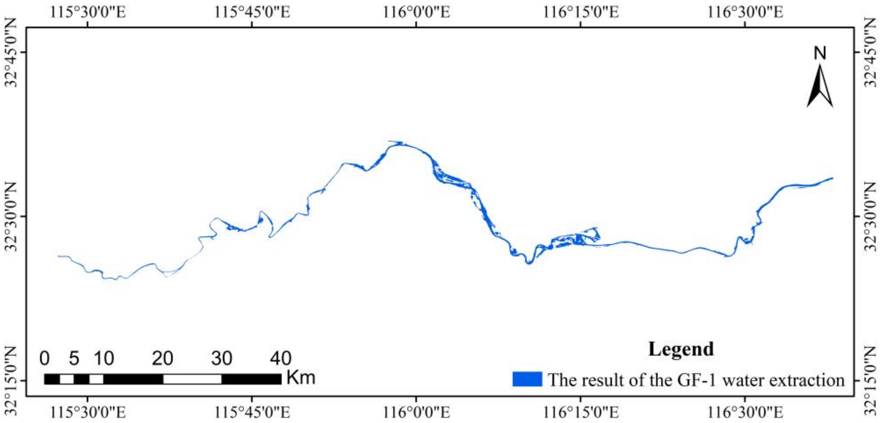
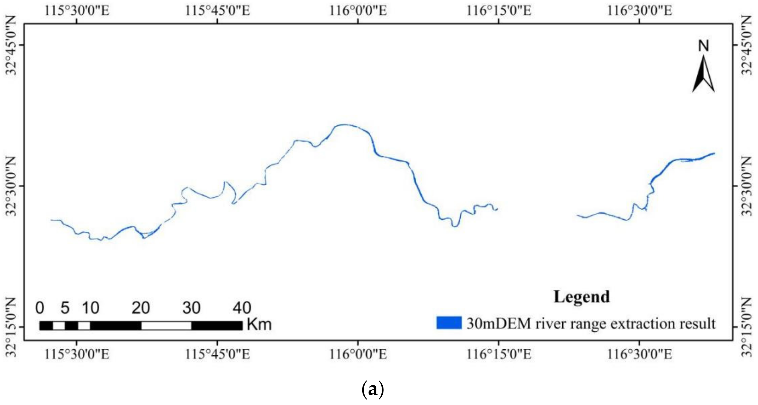
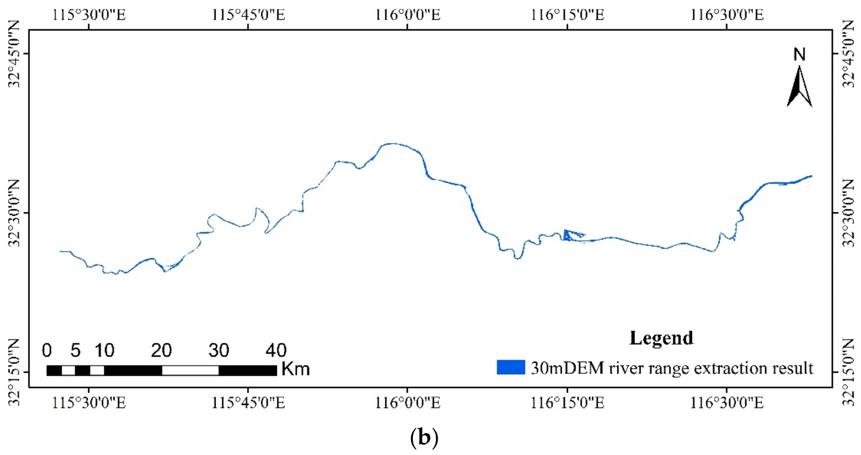
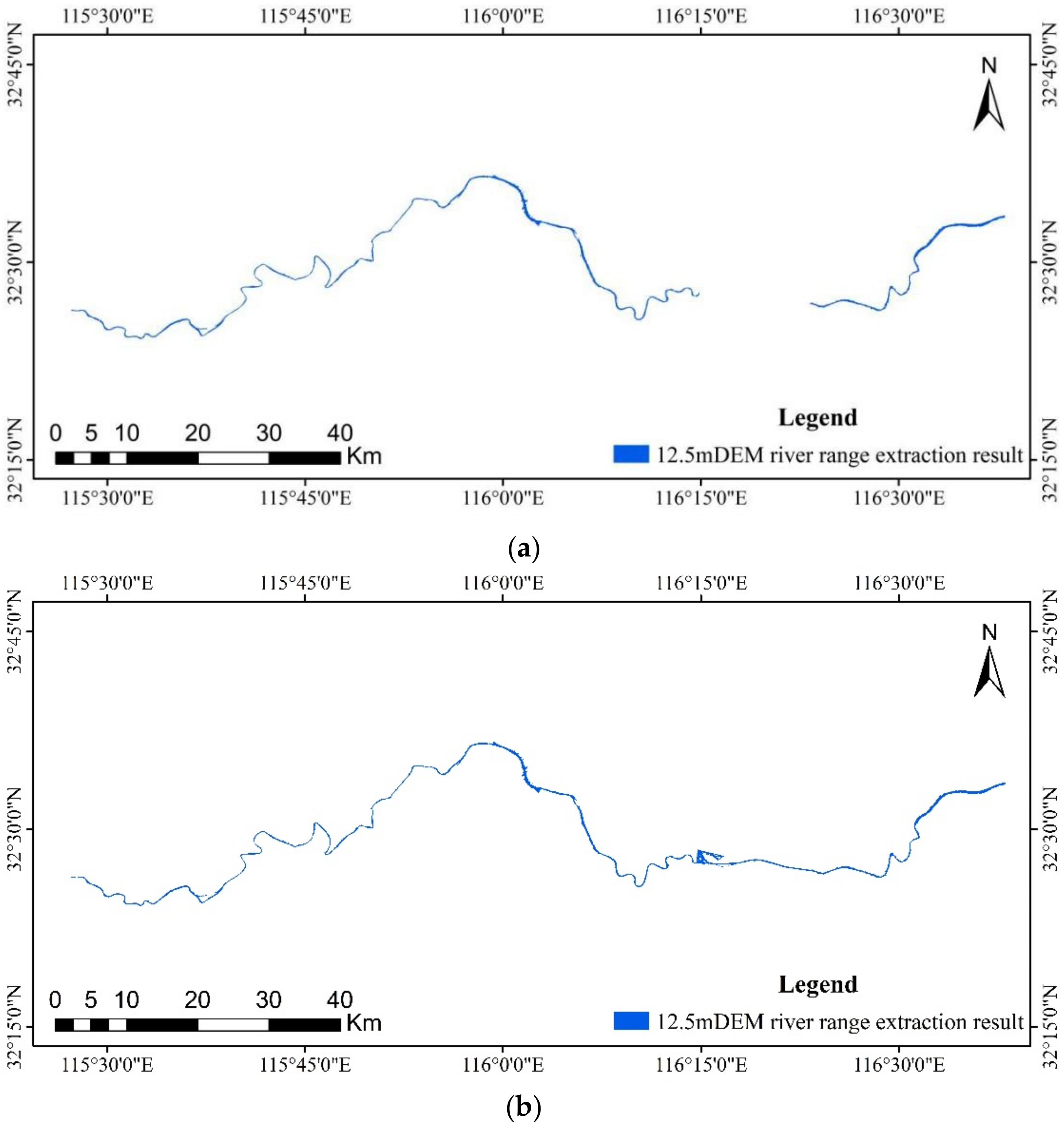
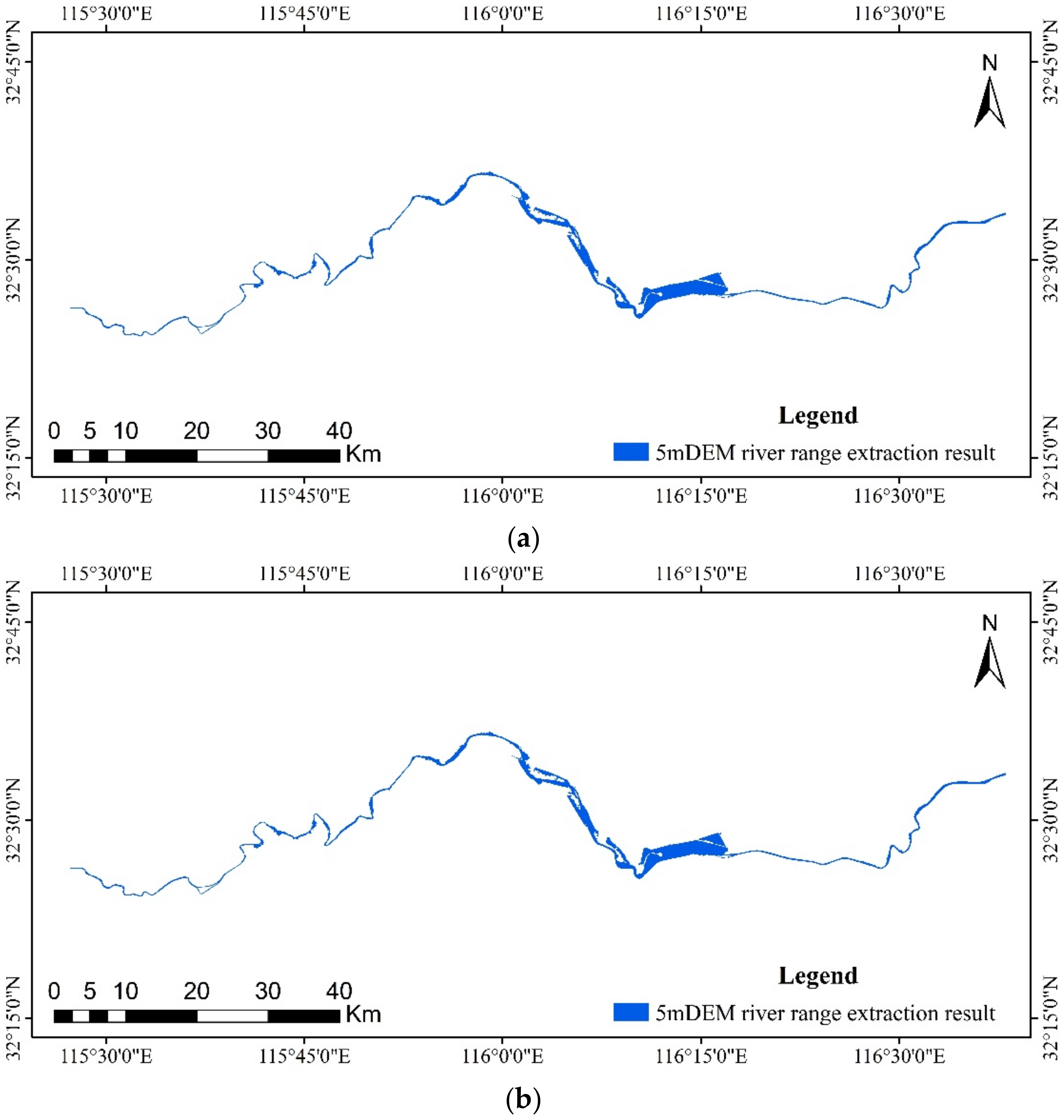
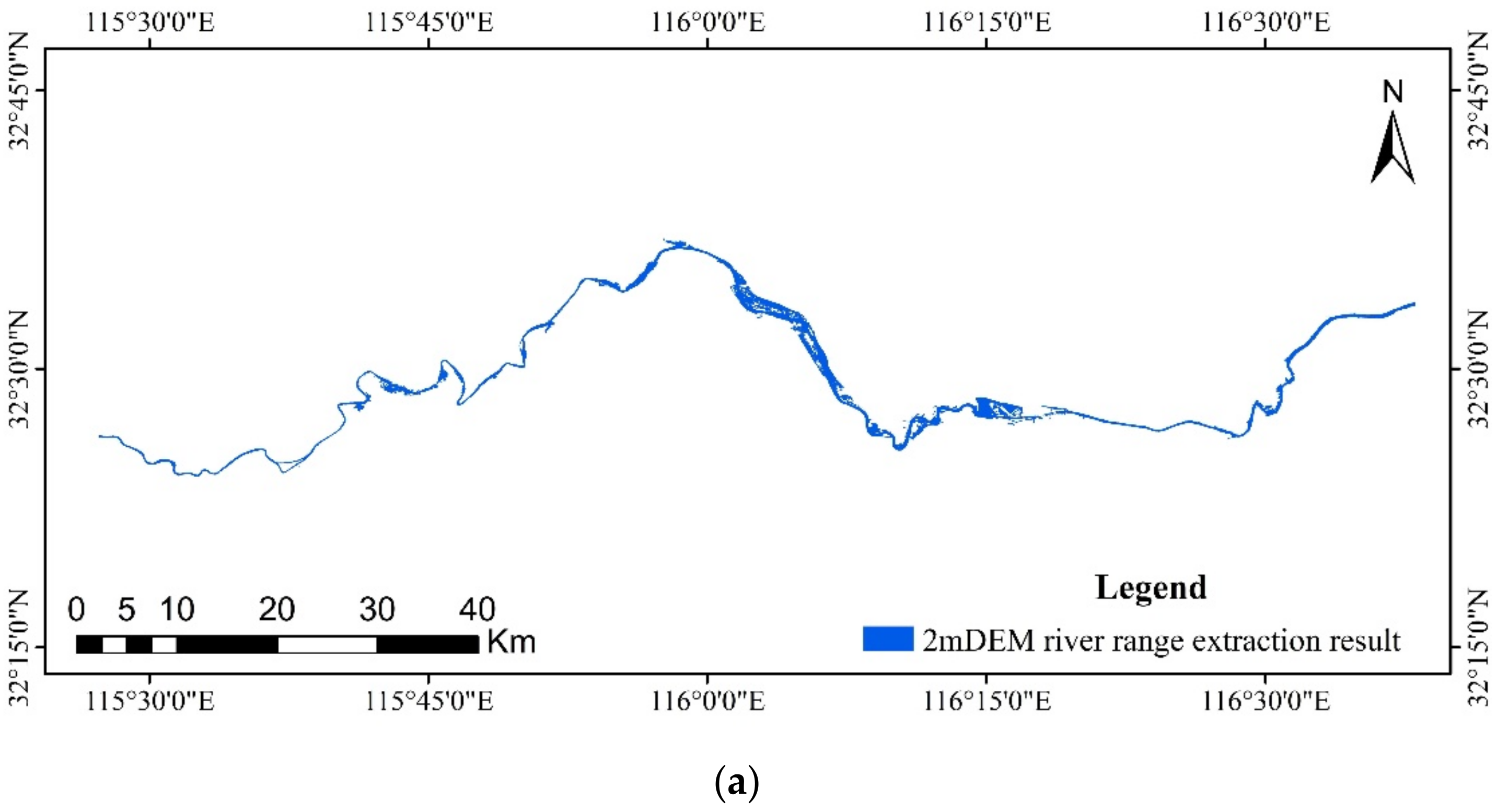
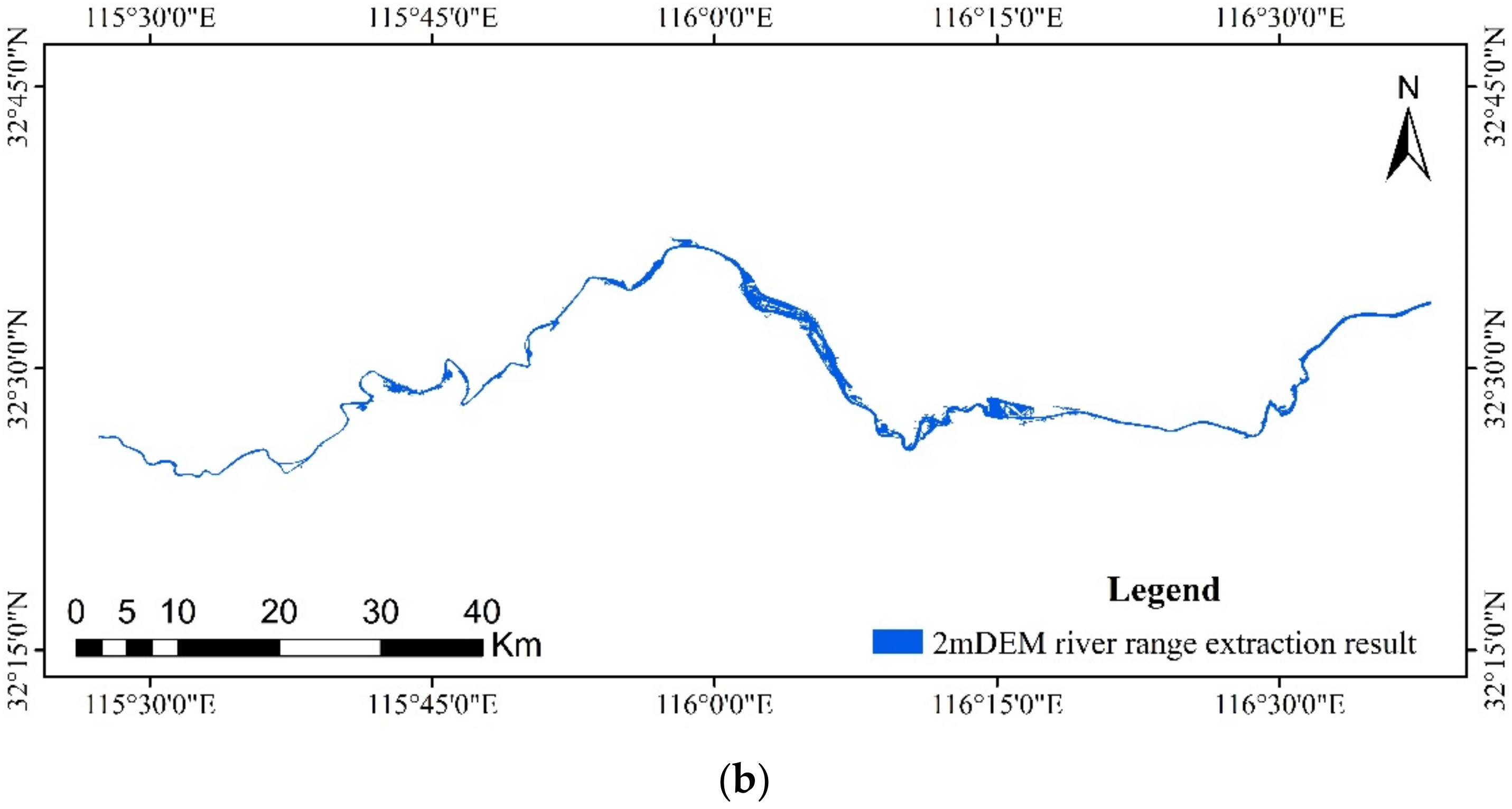
The measured ADCP section points are depicted in Figure 6, and the actual river channel range was determined based on the measured locations (Figure 7). According to the statistics, the measured channel area is 87.472 km2. Figure 8 depicts the extraction results of GF-1 data retrieved using NDWI in conjunction with OTSU, covering an area of 51,634 km2. The natural discontinuity approach was utilized to extract the river from DEMs with varying resolutions, and the water body data generated by GF-1 were utilized to update the results (Figure 9, Figure 10, Figure 11 and Figure 12). Table 2 and Table 3 display the results of the accuracy verification for the OA and Kappa coefficients.
Table 2 displays the outcomes of river extraction using only DEM data: The Kappa coefficient for DEM with a resolution of 30 m is 0.44, and the overall accuracy is 89.3%. 12.5 m DEM has an overall accuracy of 89.6% and a Kappa coefficient of 0.45. 5 m DEM has an overall accuracy of 89.3% and a Kappa coefficient of 0.56. 2 m DEM has a 90.3% overall accuracy and a Kappa coefficient of 0.59. Table 3 illustrates the combined effect of the “DEM channel extraction” model with GF-1: DEM with a resolution of 30 m has an overall accuracy of 89.6% and a Kappa coefficient of 0.47. 12.5 m DEM has an overall accuracy of 89.7% and a Kappa coefficient of 0.48. 5 m DEM has an overall accuracy of 89.3% and a Kappa coefficient of 0.56. 2 m DEM has a 90.3% overall accuracy and a Kappa coefficient of 0.59. The procedure was effective and practicable, as the Kappa coefficients were moderately consistent (0.41–0.60).
4. Discussion
This research proposes a new method that combines DEM topography data and GF-1 water extraction results, allowing for improved extraction of the channel range and good continuity of channel extraction results. When DEM extraction is employed alone, the derived results of 30 m and 12.5 m resolution DEM are incomplete and discontinuous in the middle portion. Table 2 demonstrates that the overall accuracy increases as DEM resolution increases, demonstrating that the extraction impact improves as DEM resolution grows. When DEM resolution reaches or exceeds 5 m, the area ratio of real rivers in the extraction results dramatically increases, showing that this method is more suitable for DEM resolution above 5 m.
Figure 9 and Figure 10 demonstrate that this strategy has a clear complementing effect on the DEM extraction of river channels. The accuracy verification findings indicate that after modifying GF-1 DEM using the new method (Table 3), the fraction of actual river channels in the river channel scope extraction results increases, which is superior than DEM alone. Because the tidal flat area is permanently flooded, the DEM generated from remote sensing is incapable of capturing the underwater landscape, and it is difficult to extract the river range. Consequently, GF-1 water body extraction results can be used to extract the channel range of tidal flat reach, and GF-1 results can be utilized to change the channel range extracted from DEM in order to increase its accuracy.
In contrast, when DEM is combined with GF-1 water data, the extraction effect of DEM with a resolution of less than or equal to 12.5 m is greatly enhanced. As illustrated in Figure 9 and Figure 10, this method clearly complements DEM extraction for river channel. When employing DEM extraction alone, the river extraction of the intermediate 30 M and 12.5 m DEMs is insufficient and characterized by large discontinuities. According to Table 2 and Table 3, the Kappa coefficient of GF-1 alone is 0.51, whereas the Kappa coefficients of 30 m DEM and 12.5 m DEM combined with GF-1 water body values are 0.47 and 0.48, respectively. The percentage of genuine rivers in the 30 m DEM and 12.5 m DEM extraction results is comparable to the GF-1 extraction alone. When DEM resolution is inferior to GF-1 resolution, GF-1 resolution is superior on its own. However, when the resolution approaches 5 m or greater, the new method does not provide a significant improvement over DEM alone. However, because the Jenks natural breaks classification approach requires grid partitioning for river channel extraction in such a large region, it is best suited for river channel extraction of high-precision DEM in localized areas. Therefore, DEM channel extraction paired with GF-1 is appropriate for DEM data with a lower resolution than GF-1, whereas DEM channel extraction based on Jenks natural breaks classification alone is more appropriate for high-precision DEM river range extraction in localized areas.
Compared to the method of substituting channel scope with water surface [5,6,7], this method is more accurate. Compared to the extraction of riparian line utilizing joint gray threshold segmentation, contour form recognition, and a deep neural network model [8,9,10] for photos, the approach described in this research is less complicated and more efficient. However, it is still necessary to improve the accuracy of the method.
5. Conclusions
A DEM channel extraction approach is proposed based on DEM and GF-1 data by integrating Jenks natural breaks classification with digital elevation model (DEM), and remote sensing is utilized in conjunction with GF-1 to extract river range. The effect of extracting river range from DEM at varying resolutions is investigated, and the following conclusions are drawn:
- A new method for remote sensing river range extraction based on DEM and GF-1 data is proposed by merging Jenks natural breaks classification with digital elevation model. The overall accuracy is better than 85%, and the Kappa coefficient (0.41–0.60) is moderately consistent, showing that the procedure is viable and successful;
- The extraction accuracy grows as DEM resolution increases, and the higher the DEM resolution, the better the extraction effect;
- When DEM resolution is lower than GF-1 resolution, GF-1 alone has better effect;
- The new method combining DEM channel extraction with GF-1 is more appropriate for DEM data with a DEM resolution of 5 m or higher.
- The DEM channel extraction method based solely on Jenks natural breaks classification method is better suited for obtaining high-precision DEM channel ranges in small regions.
In conclusion, it is possible to employ GF-1 water body extraction results to complement DEM river range extraction results, but not for plain areas. On the one hand, the plain area’s topography is not clear; on the other hand, because many rivers in the plain area contain a high number of perennial water pools, water extraction data to complement channel scope would increase the area of non-channel, resulting in inaccuracies. The Jenks natural breaks classification approach based on DEM can be used to extract river range; however, it is more suitable for hilly and mountainous regions with evident terrain changes. Other methods must be studied further for DEMs with medium and low accuracy in order to quickly extract the scope of a river.
Author Contributions
Conceptualization, R.G., W.S., C.L.; methodology, R.G., W.S., Y.L.; resources, X.P., Y.L.; investigation, X.P.; data curation, Y.L., L.C.; writing-original draft preparation, R.G.; writing-review and editing, R.G., Y.L.; project administration, W.S.; funding acquisition, W.S., C.L. All authors have read and agreed to the published version of the manuscript.
Funding
This research was funded by the National Natural Science Foundation of China, grant number 42142029; Key project of China Institute of Water Resources and Hydropower, grant number WH0145B042022, and Liaoning Province “Xingliao Talents Plan” project, grant number XLYC2002007.
Institutional Review Board Statement
Not applicable.
Informed Consent Statement
Not applicable.
Data Availability Statement
Not applicable.
Acknowledgments
We are grateful to those involved in data processing and manuscript writing revision.
Conflicts of Interest
The authors declare no conflict of interest.
Abbreviations
| DEM | Digital Elevation Model |
| GF-1 | GF-1 satellite |
References
- Shanxi Lingqiu Black Branch Provincial Nature Reserve Authority. In Natural Ecological Protection Noufangi; Chinese Forestry Publishing House: Beijing, China, 2013.
- Huan, W.U.; Yong-Hong, Y.I.; Wang, X. A River Bank Extracting Algorithm Based on Active Contour Model from High-Resolution Satellite Images. Remote Sens. Technol. Appl. 2006, 21, 407–413. [Google Scholar] [CrossRef]
- Gueneralp, I.; Filippi, A.M.; Hales, B.U. River-Flow Boundary Delineation from Digital Aerial Photography and Ancillary Images Using Support Vector Machines. GISci. Remote Sens. 2013, 50, 1–25. [Google Scholar] [CrossRef]
- Milad, N.J.; Alfonso, V. Reconstruction of River Boundaries at Sub-pixel Resolution: Estimation and Spatial Allocation of Water Fractions. Int. J. Geo Inf. 2017, 6, 383. [Google Scholar] [CrossRef] [Green Version]
- Yao, F.; Wang, C.; Dong, D.; Luo, J.; Shen, Z.; Yang, K. High-Resolution Mapping of Urban Surface Water Using ZY-3 Multi-spectral Imagery. Remote Sens. 2015, 7, 12336–12355. [Google Scholar] [CrossRef] [Green Version]
- Huang, C.; Chen, Y.; Zhang, S.; Wu, J. Detecting, Extracting, and Monitoring Surface Water from Space Using Optical Sensors: A Review. Rev. Geophys. 2018, 56, 333–360. [Google Scholar] [CrossRef]
- Yuan, X.Z.; Jiang, H.; Chen, Y.Z.; Wang, X. Extraction of Water Body Information Using Adaptive Threshold Value and OTSU Algorithm. Remote Sens. Inf. 2016, 31, 36–42. [Google Scholar] [CrossRef]
- Guo, Y.; Wang, Y.H.; Liu, C.P.; Gong, S.R.; Ji, Y. Bankline Extraction in Remote Sensing Images Using Principal Curves. J. Commun. 2016, 37, 80–89. [Google Scholar] [CrossRef]
- He, Z.; Li, C.; Zhang, L.; Jie, S. River Channel Extraction by Combining Grey Threshold Segmentation and Contour Form Recognition. J. Electron. Meas. Instrum. 2014, 28, 1288–1296. [Google Scholar] [CrossRef]
- Ni, L.; Zhishun, W.; Lin, W.; Zhao, J. River-Net: A Novel Neural Network Model for Extracting River Channel Based on Refined-Lee Kernel. J. Radars. 2021, 10, 324–334. [Google Scholar] [CrossRef]
- Zaidi, S.M.; Akbari, A.; Gisen, J.I.; Kazmi, J.H.; Gul, A.; Fhong, N.Z. Utilization of Satellite-Based Digital Elevation Model (DEM) for Hydrologic Applications: A Review. J. Geol. Soc. India 2018, 92, 329–336. [Google Scholar] [CrossRef]
- Barták, V. How to Extract River Networks and Catchment Boundaries from DEM: A Review of Digital Terrain Analysis Techniques. J. Landsc. Stud. 2009, 2, 57–68. [Google Scholar]
- O’Callaghan, J.F.; Mark, D.M. The Extraction of Drainage Networks from Digital Elevation Data. Comput. Vis. Graph. Image Process. 1984, 28, 323–344. [Google Scholar] [CrossRef]
- Lun, W.U.; Wang, D.M.; Zhang, Y. Research on the Algorithms of the FLow Direction Determination in Ditches Extraction Based on Grid DEM. J. Image Graph. 2006, 11, 998–1003. [Google Scholar] [CrossRef]
- Yang, H.; Cao, J. Analysis of Basin Morphologic Characteristics and Their Influence on the Water Yield of Mountain Watersheds Upstream of the Xiongan New Area, North China. Water 2021, 13, 2903. [Google Scholar] [CrossRef]
- Wu, J.; Guo, K.; Wang, M.; Xu, B. Research and Extraction of the Hydrological Characteristics Based on GIS and DEM; IEEE Publications: New York, NY, USA, 2011. [Google Scholar] [CrossRef]
- Colombo, R.; Vogt, J.V.; Soille, P.; Paracchini, M.L.; de Jager, A. Deriving River Networks and Catchments at the European Scale from Medium Resolution Digital Elevation Data. Catena 2007, 70, 296–305. [Google Scholar] [CrossRef]
- Dong, P.; Zhong, R.; Xia, J.; Tan, S. A Semiautomated Method for Extracting Channels and Channel Profiles from Lidar-Derived Digital Elevation Models. Geosphere 2020, 16, 806–816. [Google Scholar] [CrossRef] [Green Version]
- Muthusamy, M.; Casado, M.R.; Butler, D.; Leinster, P. Understanding the Effects of Digital Elevation Model Resolution in Urban Fluvial Flood Modelling. J. Hydrol. 2021, 596, 126088. [Google Scholar] [CrossRef]
- Coulson, M.R.C. In the Matter of Class Intervals for Choropleth Maps: With Particular Reference to the Work of George F Jenks. Cartogr. Int. J. Geogr. Inf. Geovis. 1987, 24, 16–39. [Google Scholar] [CrossRef]
- Jenks, G.F. Generalization in Statistical Mapping. Ann. Assoc. Am. Geogr. 1963, 53, 15–26. [Google Scholar] [CrossRef]
- Chen, J.; Yang, S.T.; Li, H.W.; Zhang, B.; Lv, J.R. Research on Geographical Environment Unit Division Based on the Method of Natural Breaks (Jenks). Int. Arch. Photogramm. Remote Sens. Spatial Inf. Sci. 2013, XL-4/W3, 47–50. [Google Scholar] [CrossRef] [Green Version]
- McFeeters, S.K. The Use of the Normalized Difference Water Index (NDWI) in the Delineation of Open Water Features. Int. J. Remote Sens. 1996, 17, 1425–1432. [Google Scholar] [CrossRef]
- Otsu, N. A Threshold Selection Method from Gray-Level Histograms. IEEE Trans. Syst. Man Cybern. 1979, 9, 62–66. [Google Scholar] [CrossRef] [Green Version]
- Hollingsworth, D.; The Workflow Reference Model, Workflow Management Coalition (WFMC). Document No. TC00-1003, No. 1.1. 1995. Available online: www.pa.icar.cnr.it/cossentino/ICT/doc/D12.1%20-%20Workflow%20Management%20Coalition%20-%20The%20Workflow%20Reference%20Model.pdf (accessed on 17 March 2022).
- Ji, L.; Zhang, L.; Wylie, B. Analysis of Dynamic Thresholds for the Normalized Difference Water Index. Photogramm. Eng. Remote Sens. 2009, 75, 1307–1317. [Google Scholar] [CrossRef]
- Goh, T.Y.; Basah, S.N.; Yazid, H.; Aziz Safar, M.J.; Ahmad Saad, F.S. Performance Analysis of Image Thresholding: Otsu Technique. Measurement 2018, 114, 298–307. [Google Scholar] [CrossRef]
- Sahoo, P.K.; Soltani, S.; Wong, A.K.C. A Survey of Thresholding Techniques. Comput. Vis. Graph. Image Process. 1988, 41, 233–260. [Google Scholar] [CrossRef]
Figure 1.
Map of the geographical location of the river studied (the geographical position of the Huai River in China (a), the study area is the main stream of Huaihe River from Huaibin station to Lutaizi station, which flows through four cities and seven counties (b).
Figure 1.
Map of the geographical location of the river studied (the geographical position of the Huai River in China (a), the study area is the main stream of Huaihe River from Huaibin station to Lutaizi station, which flows through four cities and seven counties (b).

Figure 2.
Research route.

Figure 3.
Example of DEM histogram (DEM histogram divided into four categories by natural discontinuity method).
Figure 3.
Example of DEM histogram (DEM histogram divided into four categories by natural discontinuity method).

Figure 4.
GF-1 data in the study area (the data used is gaofen-1 data on 30 May 2021).

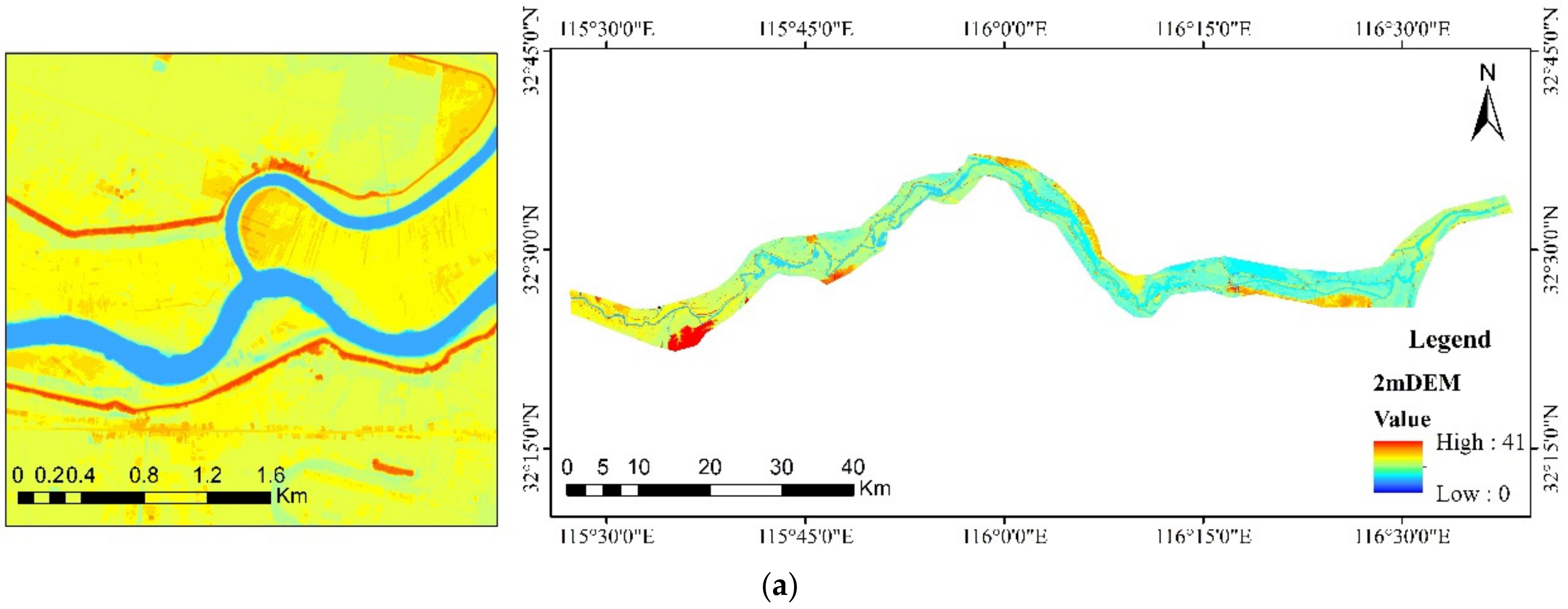
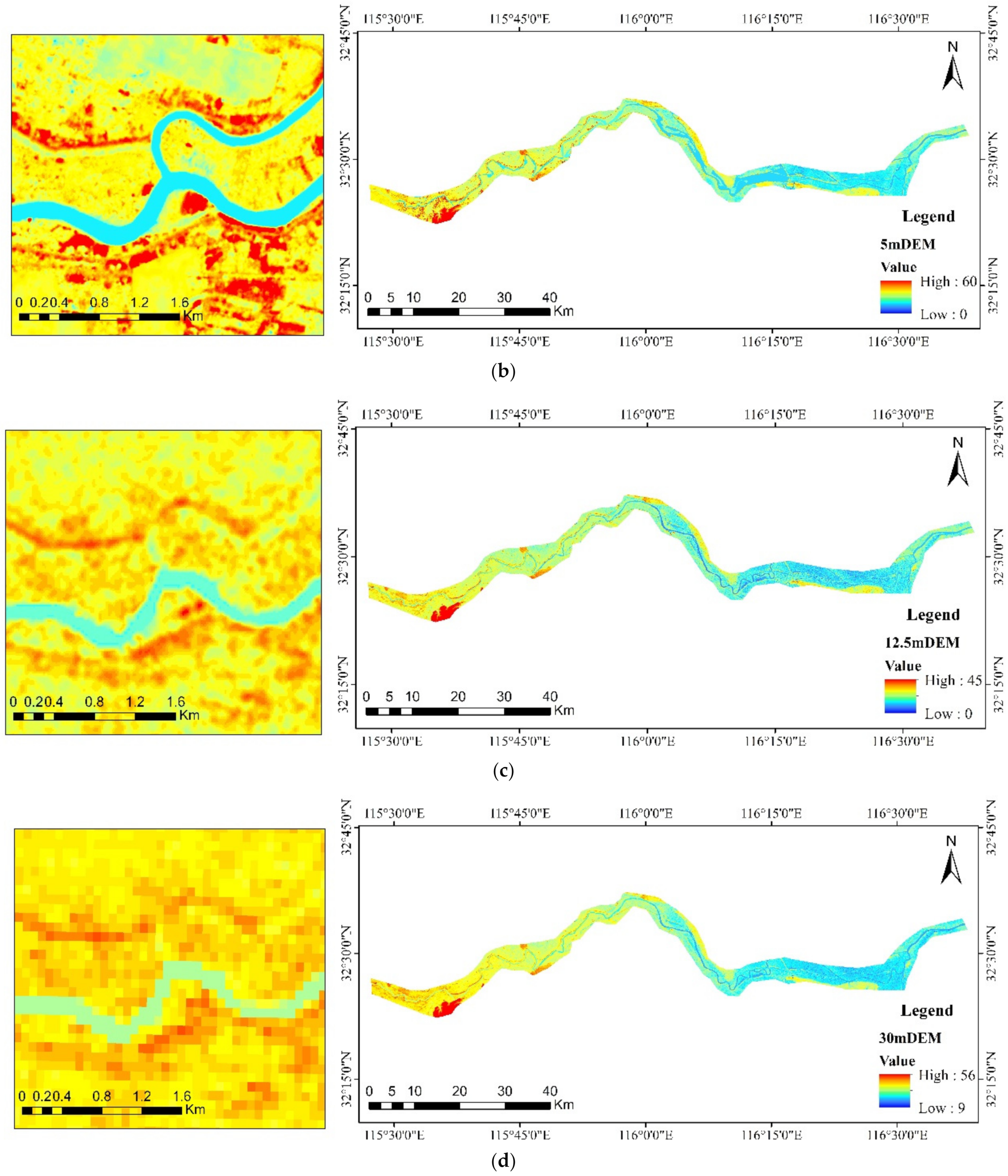
Figure 5.
DEM data with resolutions of (a) 2 m, (b) 5 m, (c) 12.5 m, (d) and 30 m, respectively. Resolution is the smallest unit of measurement used to record data and is used to describe the area represented by a pixel point in the image. For example, DEM with 2 m resolution indicates that the area of a pixel in the DEM data is 2 m × 2 m).


Figure 6.
Measured points on river section (the upper left corner of the figure is a point zoom display).
Figure 6.
Measured points on river section (the upper left corner of the figure is a point zoom display).

Figure 7.
Measured channel range.

Figure 8.
GF-1 water extraction results.

Figure 9.
(a) Extraction results of 30 m DEM channel and (b) extraction results combined with GF-1 data.
Figure 9.
(a) Extraction results of 30 m DEM channel and (b) extraction results combined with GF-1 data.


Figure 10.
(a) Extraction results of 12.5 m DEM channel and (b) extraction results combined with GF-1 data.
Figure 10.
(a) Extraction results of 12.5 m DEM channel and (b) extraction results combined with GF-1 data.

Figure 11.
(a) Extraction results of 5 m DEM channel and (b) the results combined with GF-1 data.

Figure 12.
(a) Extraction results of 2 m DEM channel and (b) the results combined with GF-1 data.


Table 1.
Data specific information.
| Data | Resolution | Data Source |
|---|---|---|
| DEM | 30 m (2020) | Geospatial Data Cloud (https://www.gscloud.cn/, (accessed on 17 March 2022)) |
| 12.5 m (2021) | Geospatial Data Cloud | |
| 5 m (2021) | China Centre for Resources Satellite Data and Application | |
| 2 m (April 2021) | Laser point cloud data extraction results | |
| GF-1 (30 May 2021) | 16 m | China Centre for Resources Satellite Data and Application |
| River section data | / | ADCP measurement results |
Table 2.
Statistics of river channel range extraction results of DEM with different resolutions.
| Data | Real Value | Channel Area (km2) | Non-Channel Area (km2) | OA | Kappa | |
|---|---|---|---|---|---|---|
| Predictive Value | ||||||
| 30 m DEM | Channel area (km2) | 28.25 | 1.69 | 89.3% | 0.44 | |
| Non-channel area (km2) | 59.22 | 482.14 | ||||
| 12.5 m DEM | Channel area (km2) | 29.17 | 1.32 | 89.6% | 0.45 | |
| Non-channel area (km2) | 58.29 | 482.51 | ||||
| 5 m DEM | Channel area (km2) | 49.59 | 23.00 | 89.3% | 0.56 | |
| Non-channel area (km2) | 37.87 | 460.82 | ||||
| 2 m DEM | Channel area (km2) | 49.36 | 17.42 | 90.3% | 0.59 | |
| Non-channel area (km2) | 38.11 | 466.41 | ||||
| GF-1 | Channel area (km2) | 39.38 | 12.25 | 89.4% | 0.51 | |
| Non-channel area (km2) | 48.09 | 471.58 | ||||
Table 3.
Statistics of river channel range extraction results of DEM with different resolutions (combined with GF-1 water extraction results).
Table 3.
Statistics of river channel range extraction results of DEM with different resolutions (combined with GF-1 water extraction results).
| Data | Real Value | Channel Area (km2) | Non-Channel Area (km2) | OA | Kappa | |
|---|---|---|---|---|---|---|
| Predictive Value | ||||||
| 30 m DEM | Channel area (km2) | 31.43 | 3.61 | 89.6% | 0.47 | |
| Non-channel area (km2) | 56.05 | 480.22 | ||||
| 12.5 m DEM | Channel area (km2) | 32.12 | 3.26 | 89.7% | 0.48 | |
| Non-channel area (km2) | 55.36 | 480.57 | ||||
| 5 m DEM | Channel area (km2) | 49.59 | 23.01 | 89.3% | 0.56 | |
| Non-channel area (km2) | 37.87 | 460.82 | ||||
| 2 m DEM | Channel area (km2) | 49.48 | 17.42 | 90.3% | 0.59 | |
| Non-channel area (km2) | 37.99 | 466.41 | ||||
Publisher’s Note: MDPI stays neutral with regard to jurisdictional claims in published maps and institutional affiliations. |
© 2022 by the authors. Licensee MDPI, Basel, Switzerland. This article is an open access article distributed under the terms and conditions of the Creative Commons Attribution (CC BY) license (https://creativecommons.org/licenses/by/4.0/).
Share and Cite
MDPI and ACS Style
Gui, R.; Song, W.; Pu, X.; Lu, Y.; Liu, C.; Chen, L. A River Channel Extraction Method Based on a Digital Elevation Model Retrieved from Satellite Imagery. Water 2022, 14, 2387. https://doi.org/10.3390/w14152387
AMA Style
Gui R, Song W, Pu X, Lu Y, Liu C, Chen L. A River Channel Extraction Method Based on a Digital Elevation Model Retrieved from Satellite Imagery. Water. 2022; 14(15):2387. https://doi.org/10.3390/w14152387
Chicago/Turabian StyleGui, Rongjie, Wenlong Song, Xiao Pu, Yizhu Lu, Changjun Liu, and Long Chen. 2022. "A River Channel Extraction Method Based on a Digital Elevation Model Retrieved from Satellite Imagery" Water 14, no. 15: 2387. https://doi.org/10.3390/w14152387
Note that from the first issue of 2016, this journal uses article numbers instead of page numbers. See further details here.