
Laboratory Study on Flow Characteristics during Solitary Waves Interacting with a Suspended Horizontal Plate

State Key Laboratory of Coastal and Offshore Engineering, Dalian University of Technology, Dalian 116023, China
*
Author to whom correspondence should be addressed.
Water 2022, 14(15), 2386; https://doi.org/10.3390/w14152386
Submission received: 8 June 2022
/
Revised: 27 July 2022
/
Accepted: 29 July 2022
/
Published: 1 August 2022
(This article belongs to the Special Issue Advances in Experimental Hydraulics, Coast and Ocean Hydrodynamics)
Abstract
:A series of laboratory experiments were conducted to investigate the 2–D kinematic field evolution around a suspended plate induced by solitary waves. The plate–type structure was rigid and suspended above the mean water level, while the solitary waves were generated by the wave maker to simulate the nearshore tsunami waves. The ratio of incident wave height to water depth was in the range of [0.200, 0.333], and the structural suspended height was in the range of [0.067, 0.200]. The velocity field around the deck was measured using the non–intrusive image–based PIV (Particle Image Velocimetry) method. As a result, the flow evolution was categorized into three phases: green water tongue generated, green water overtopping, and flow separation. Flow evolutions in different conditions presented obvious similarities in general but several differences in detail. The measured maximum horizontal and vertical velocities were around 1.9 C0 and 0.8 C0, respectively, where C0 is the maximum flow speed of the incident wave. Ritter’s analytical solution for the dam–break flow problem was examined and compared with the measured data. The accuracy of this solution for the present subject is significant in the period of T ∈ (0.6, 0.9). The adequate experimental data are valuable as a benchmark problem for further numerical model refinement and the improvement of fluid theory.
1. Introduction
Horizontal plates are widely used in coastal structures, such as coastal bridges which are exposed to the threat of unexpected marine disasters in the ocean. The failure of coastal bridges may result in traffic interruptions, material blockages, and rescue delays [1]. Among marine disasters, the ocean tsunami is catastrophic both for coastal people and structures. As the report of Maruyama, et al. [2] concerning the 2011 Tohoku tsunami in the Pacific Ocean demonstrates, despite the great earthquake in East Japan (magnitude of 9 on the Richter scale), most of the coastal bridges remained intact. However, these bridges were destroyed by the subsequent tsunami waves. Hence, it is becoming necessary to have a deeper understanding of the hydrodynamic processes of ocean waves impinging on plate–type structures.
In addition to tsunami waves, extreme waves are also a common marine disaster, causing complex processes on the decks of bridges and marine platforms. When big waves hit ocean structures in rough seas, a portion of the water runs up along the deck structure, violently collapses onto the frontal deck, and quickly washes over the entire deck [3,4,5,6,7,8]. This type of event, known as “green water,” has the potential to cause damage to bridges and platforms. Meanwhile, precisely estimating the kinematics of violent, multi–phase flows is still challenging [9,10,11,12]. In the past decades, to accurately describe multi–phase flow characteristics and understand the flow kinematics of the green water phenomena, several studies have been conducted using experimental [13,14,15] and numerical [16,17,18,19] methods. Additionally, Chang, et al. [20] investigated green wave impinging on a 3–D model structure using bubble image velocimetry (BIV). In this experiment, the maximum horizontal velocity for the plate impinging case is 1.44 C with C being the wave phase speed. More recently, Chuang, et al. [21] investigated green water kinematics due to wave impingements on a fixed platform experimentally in a large, deep–water basin. Both plunging breaking waves and random waves were employed in the generation of green water. Nielsen and Mayer [22] used a Navier–Stokes flow solver and the VOF scheme to simulate green water on a vessel with and without motions. Water elevations on the two–dimensional plate agreed with the experimental findings, but the extension to three–dimensional situations revealed that the three–dimensional effect is not significant. In the recent work of Yan, et al. [23], an immersed boundary method is applied to simulate the green water over a fixed plate by combining a level set method for the free water surface capturing. Their numerical model agreed well with the experimental tests in wave surface and impact pressure, and proved to be very promising for the prediction of green water problems due to its accuracy and efficiency.
For the problem of waves overtopping over the structures, some analytical solutions have been developed to better understand the phenomenon and predict the damage it may cause, one of these is the application of the dam–break model. A basic solution for dam–break under the assumption of a frictionless dry flatbed was given by Ritter [24], in which he presented the free surface profile of a collapsing rectangular column of fluid over a horizontal bed. This analytical solution has been widely used by researchers for experimental and numerical prediction of the movement of green water. Lauber and Hager [25] conducted dam–break experiments in a smooth rectangular and horizontal channel, in which the wave profiles and velocity distributions were measured. Their results indicated that the front velocity of a dam break flow reduces as time increases, which disagrees with the constant front velocity shown in the analytical solution of Ritter [24]. Buchner [26] experimentally evaluated the green water on ship–type offshore structures based on a clear description of the green water physics. He applied Stoker’s solution [27] of the dam–break model to the green water phenomena with the shallow water assumption and concluded the theoretical dam–breaking theory can help to understand the green water physics better. Yilmaz, et al. [28] developed a semi–analytical solution for a dam break flow to simulate green water problems. The result indicated that a jet–like water profile can be formulated at the forefront of the flow. However, the analytical solution is still too simple to fully elucidate the physics of green water over a deck. Ryu, et al. [29] compared the green water with the dam break flow to examine the applicability of dam–break flow models to describe green water flows. In their experiments, both the measured cross–sectional velocity and the depth–averaged velocity of overtopping water on a simplified model structure were used for comparison. The comparisons indicated that the solution of Ritter [24] for dam–break flows works well in the prediction of green water velocity despite the significant difference between these two flows. The dam–break model has also been used in various numerical simulations, e.g., the water impact and green water loading simulation using the Navier–Stokes solver [30,31,32], the improved incompressible smooth particle hydrodynamics (ISPH) method [33], and the simulation of green water flow on deck using motion equations in the Lagrangian form [34].
Despite numerous efforts have done in past decades, they mainly focused on the interaction of short–period waves with deck–type structures. Such interactions are instantaneous and different from the characteristics of tsunami waves, which present as a long–period motion [35,36,37,38,39]. In this instance, it would be more appropriate to describe the front bore of such a long wave as a solitary wave [1,40,41,42]. The research on the interaction between solitary waves and the suspended plate is still limited, most of which was focused on the impinging force. French [43] conducted a series of experiments in a 100–ft long by 2–ft deep wave tank to investigate in detail the rapidly varying pressure on a rigid, fixed, platform, strutted by the generated solitary waves. In his experiments, the maximum measured slowly varying uplift pressure head is approximately equal to the incident wave height less the soffit clearance above still water level. McPherson [44] conducted experiments using a large–scale 3–D wave basin to investigate the surge forces on the flat–plate structures. The wave force results show no strong correlation between the actual force measured and the predicted force of existing theoretical methods. Both experimental and numerical simulations were carried out by Lau, et al. [45] to investigate the tsunami forces on coastal bridge decks. The results reveal that the tsunami forces on the bridge deck are categorized into four types, i.e., impulsive, slowly varying, uplift, and additional gravity forces. Based on the field survey of the Great East Japan Earthquake on 11 March 2011, Maruyama, et al. [2] carried out an experimental investigation of tsunami forces acting on bridges, using solitary waves with the ratio of wave height to water depth from 0.13 to 0.37. Seiffert, et al. [46] conducted a series of experiments to measure the horizontal and vertical forces on a 2–D suspended plate due to solitary waves. The experimental data were compared with the computational results obtained by the CFD package OpenFOAM. Their results show that larger wave amplitudes have little effect on the vertical downward forces, as does the plate elevation.
Besides the hydrodynamic impinging force, the flow kinematics around the structure is crucial for structural optimization. By improving our understanding of the flow field, we can save structural materials and improve structural stability. For the present subject of solitary waves propagating over a suspended plate, the flow field has not been measured in the previous experimental studies, to the best of the authors’ knowledge. Only a few numerical studies have mentioned this problem. Lau, Ohmachi, Inoue and Lukkunaprasit [45] investigated the tsunami force on bridge decks using Reynolds Averaged Navier–Stokes equations (RANS). They found the height of splashes over the bridge is three times that of the incident wave. The deflected column of water collapses and falls back on the wave with a substantial amount of entrained air. Qu, et al. [47] conducted a numerical simulation on the impact of solitary waves on a bridge deck with vents, both the physical phenomena and hydrodynamic loads were simulated using an unstructured mesh, interface–capturing, incompressible flow solver. Their snapshots of the simulation showed that as the wave approaches the deck, the water–surface elevation rises, first at the front of the deck and then at its downstream side, after that the wave impacts the deck from the upstream side. Recently, Chen, et al. [48] built a numerical model based on the Reynolds–averaged Navier–Stokes (RANS) equations to dynamically simulate the interaction of solitary waves and Box–deck structures. According to their simulation results, the bridge decks separated the water wave flow into two parts. Green water occurs when the first part of the water flows above the bridge deck surfaces. Under the influence of gravity, the other part of the water wave is transmitted beneath the bottom of the decks. When the first part of the wave above the bridge deck flows back to the wave tank at the rear of the deck, the water surface elevation is equal to that of the deck surface.
Overall, the study on the kinematics during the impact of solitary waves on the plate above water is very limited, especially for experimental research. To fill the knowledge gap, in the present study, we focus on the flow evolution around a suspended fixed plate–type model in the laboratory. The solitary waves were generated to simulate a nearshore tsunami, the ratio of wave height to water depth is limited within the range of 6/30 to 10/30. Several structural suspended heights are employed in the range of 2/30 h to 6/30 h (h is water depth). Besides, a non–intrusive image–based measuring technique (Particle Image Velocimetry, PIV) was used to measure the characteristics of two–dimensional flow evolution around the suspended plate. In this paper, flow evolution around the plate is described firstly and the timeline of different stages is illuminated. Then, the change of normalized maximum velocity is analyzed. Whereafter, we will present the effects of wave height and the model’s suspended height on the flow patterns. Finally, as a common formula to describe dam break, Ritter’s solution was compared with measured velocity data, to examine the applicability of the dam–break solution to predict flow velocity in the solitary wave condition.
2. Experimental Set–Up
2.1. Experimental Apparatus and Model Structure
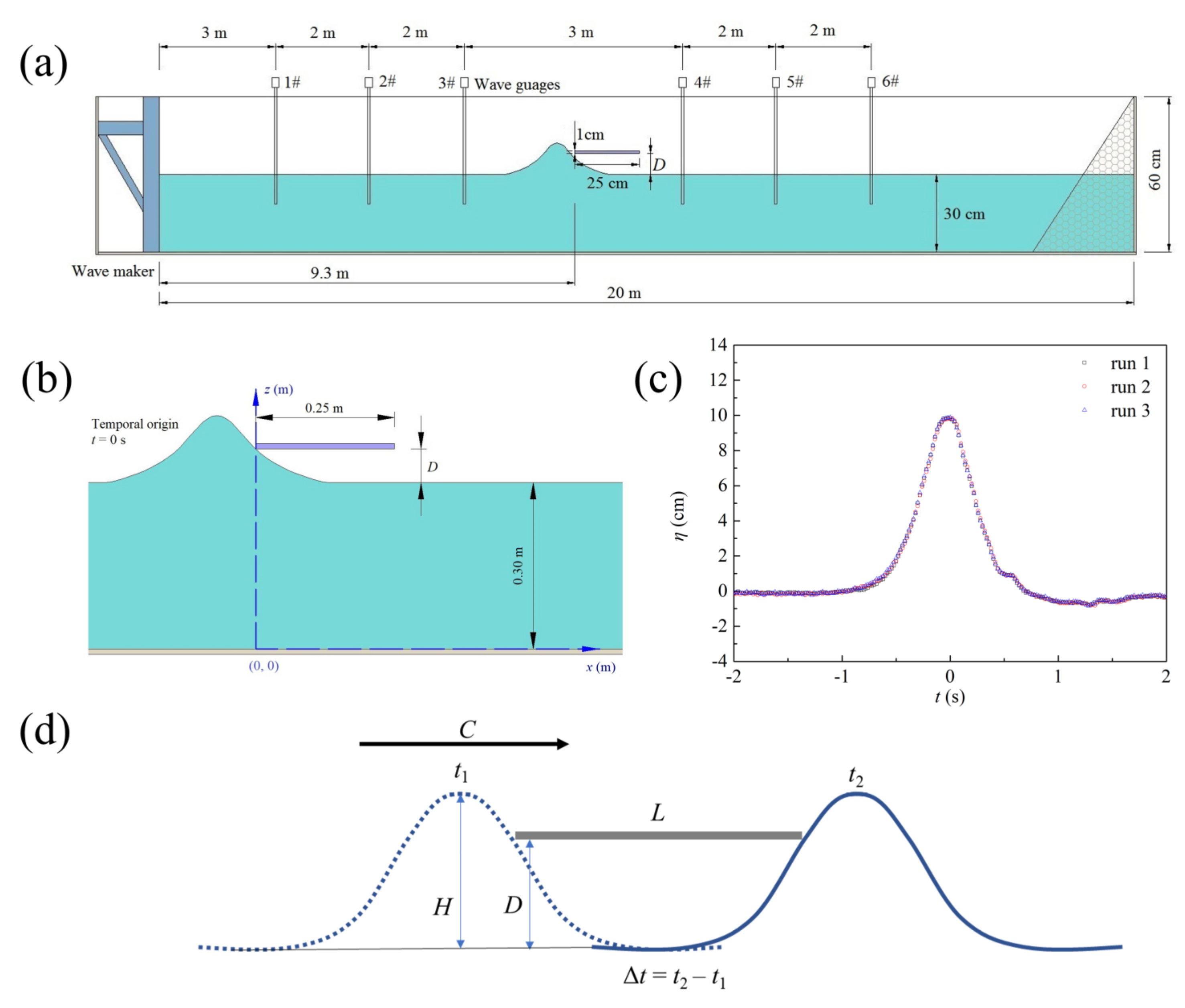
The experiment was carried out in a glass–walled wave flume, which has dimensions of 20 m in length, 0.45 m in width, and 0.6 m in height. A schematic diagram of the wave flume is illustrated in Figure 1a. The model plate is a two–dimensional structure, with a dimension of 0.25 m in length (L), 10 mm in thickness, and spanning the width of the tank. The plate was suspended at several fixed heights above the flume bottom without any supporting frames inside the flume. It should be noted that the plate has a high level of rigidity and is firmly attached to the flume wall. For the whole experiment, it can be assumed that the plate is rigid. Indeed, the displacement of the plate recorded by the high–speed camera is too small to be seen by the human eye.
Using Goring’s procedure [49], a solitary wave was generated by a programmable servo–controlled piston–type wavemaker at one end of the wave flume. A sloping beach of 1/5 (vertical/horizontal) covered with layers of horsehair was installed at the other end of the flume to mitigate wave reflection [50].
The following theoretical solution proposed by Korteweg and De Vries [51] is used to generate the solitary waves in the flume:
where η denotes the free surface elevation above the still water level; x and t denote the streamwise direction and time; H = wave height; h = water depth; and c = wave celerity that can be calculated as .
Assuming the waves traveling in a single direction, Korteweg and De Vries [51] derived Equation (1) from the Boussinesq equation [52], which assumes the flow is inviscid, irrotational, incompressible and the horizontal wavelength is large compared to the depth (l > h).
In our present experiments, the coordinates are shown in Figure 1b. Additionally, the temporal origin t = 0 s is defined as the moment when the solitary wave is just touching the front edge of the plate.
Along the wave flume, the free–surface elevations were recorded by six capacitance–type wave gauges. The repeatability of the incident wave was confirmed by comparing the surface elevation measurements in the absence of the model by conducting the experiments three times. The results of the tested surface elevation are shown in Figure 1c.
2.2. Velocity Measurements by PIV
A high–speed PIV (Particle Image Velocimetry) equipment was used to measure the two–dimensional velocity field surrounding the structure. The PIV system consists of a high–speed CMOS camera, a solid–state laser, and tracer particles mixed in the water.
The 2–D measurement area was illuminated by an 8 W solid–state laser with a 532 nm wavelength. A 1.5 mm thick light sheet was formed and spread into the wave flume vertically along the flume centerline through a cylindrical lens. Borosilicate glass particles of 8–12 μm in diameter were chosen as the seeding material, which was uniformly introduced into the water for velocity field measurement. The particles have a density of 1.1 g/cm3 and keep well suspended and fluid–following in water. A high–speed complementary metal–oxide–semiconductor (CMOS) camera (PCO.dmaxS4) with a resolution of 2016 × 2016 pixels, 12–bit dynamic range, and 1000–Hz framing rate was used to capture the particle–laden images.
Velocity fields were calculated through the cross–correlation analysis. Interrogation windows of 32 × 32 pixels with 50% overlap between adjacent windows were used in the analysis. For the experimental case, 16 runs were repeated, and the ensemble averaged both for the velocity and free surface measurements to reduce measurement uncertainty. It is worth declaring that most of the measurement areas in the experiment are bubble–free water or low aeration areas. At these positions, we can measure the velocity through the motion of particles and the texture motion of the interface. However, in the very high aeration area of fluid separation under the plate, the velocity of fluid movement has not been measured quantitatively, the area of this part is relatively small and has a relatively limited impact on the wave on the plate.
2.3. Experimental Conditions
A total of five experimental cases are tested throughout our experiments, in which the main distinguishing parameters are structural suspended heights and incident wave heights. Table 1 lists the principal parameters of wave conditions and the setting of the plate model. Three relative wave heights H/h = 0.33, 0.27, and 0.20 are employed and three relative suspended heights covering 0.067 to 0.200 are tested.
To analyze the dimensionless velocity variation of different cases, the maximum free stream velocity of the incident wave is calculated and listed in Table 1. Considering the weak nonlinearity [53], and in the assumption of long wave theory (l > h), the velocity distribution along the depth can be expressed as
According to the experimental results of Lee, et al. [54], the maximum fluid velocity appears at the peak of the solitary wave, i.e.,
Substituting Equation (4) to the velocity distribution of Equations (2) and (3), the maximum fluid velocity of the incident wave can be expressed as,
Due to the varying parameters, the interaction process of waves of structures may be difficult to compare. Hence, a normalized time is employed, which considers factors of wave height and structural suspended height, as follows
where Δt is the geometric period of an incident wave passing through the plate, details of which can refer to in the sketch map in Figure 1d.
3. Results and Discussion
3.1. Evolution of Flow Structures
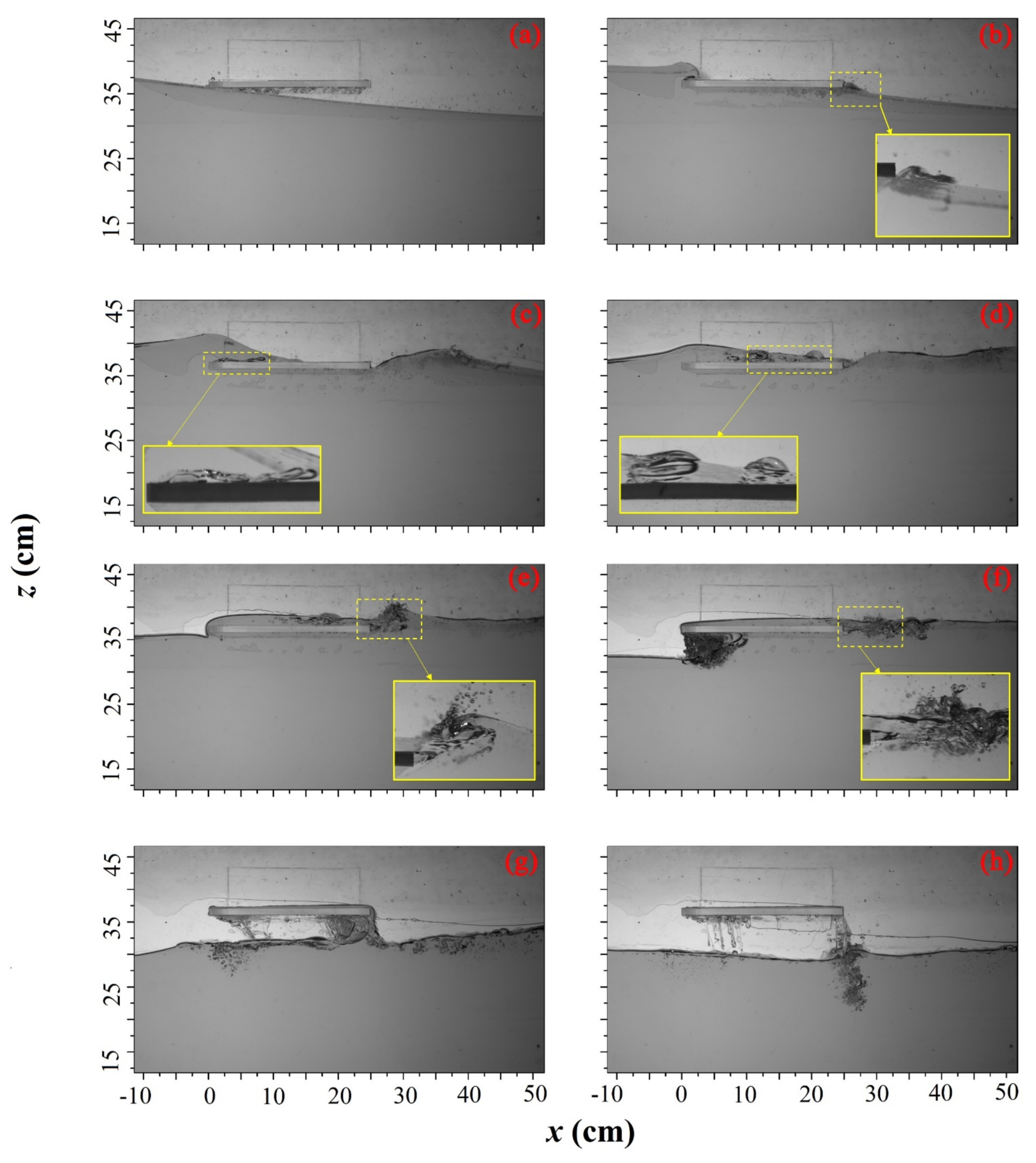
For the lash of waves on suspended structures, the flow kinematics are usually complex and important. Here, Case 1 (D/h = 6/30, H/h = 10/30) is chosen as a representative case to analyze the basic hydrodynamic process of flow evolutions. Through the high–speed camera, the green water flow generated during large solitary waves impinging on the plate structure was recorded. Sample raw images of green water on the plate are presented in Figure 2 to illustrate the physical process. To illustrate the details of bubble structure more clearly, several close–ups of the aerated flow surface are presented. It should be noted that the two–phase flow inside the aerated region exhibits obvious three–dimensional characteristics, which are only described qualitatively here. The flow fields measured by PIV are 2–D profiles without considering the movement of the bubble region. The flow was illuminated by a 20–w led uniform light source projected from the back, which was attached to the back glass wall of the flume. Please note that the wave in front of the structure is aerated and contains air bubbles. Bubbles are subject to the surface tension effect, which may not be amplified by the Froude similarity [21]. Therefore, the air–water mixture flow in this study may suffer from the scale effect.
Figure 2a shows the moment when the front side of the wave is just contacting the structure (T = 0). The wavefront surface is smooth, as the solitary wave has not broken up. After the impact, a jet flow run–up vertically along the front face of the structure (Figure 2b). Under the influence of gravity, the water tongue turned over and dropped down on the front of the upper surface. At T = 0.42, as shown in Figure 2c, the air bubbles involved at the front of the plate begin to break, as the water under the deck’s bottom appears to extrude from the end of the plate. This extrusion phenomenon, which was not mentioned in the previous studies, may induce a significant impact on the bottom of the plate. With the wave propagating, the green water overtopping moves downstream rapidly. As shown in Figure 2d, the area of green water collides with the water behind the plate. The collision of these two parts of the water body occurs on the back side of the plate. At T = 0.74, this collision of water bodies evolves into the fluid splash phenomenon as shown in Figure 2e. The air admixture increased again on the back side of the plate as a result of this. After T = 0.74, the main body of the wave crest gradually starts to separate from the plate. First, in the weather side area of the plate, the body of water begins to separate from the plate as shown in Figure 2f. This process involves a strong gas–liquid admixture phenomenon. After that, the body of water attached to the plate gradually detaches, as the water flows down mainly from the end edge of the plate, see Figure 2g,h.
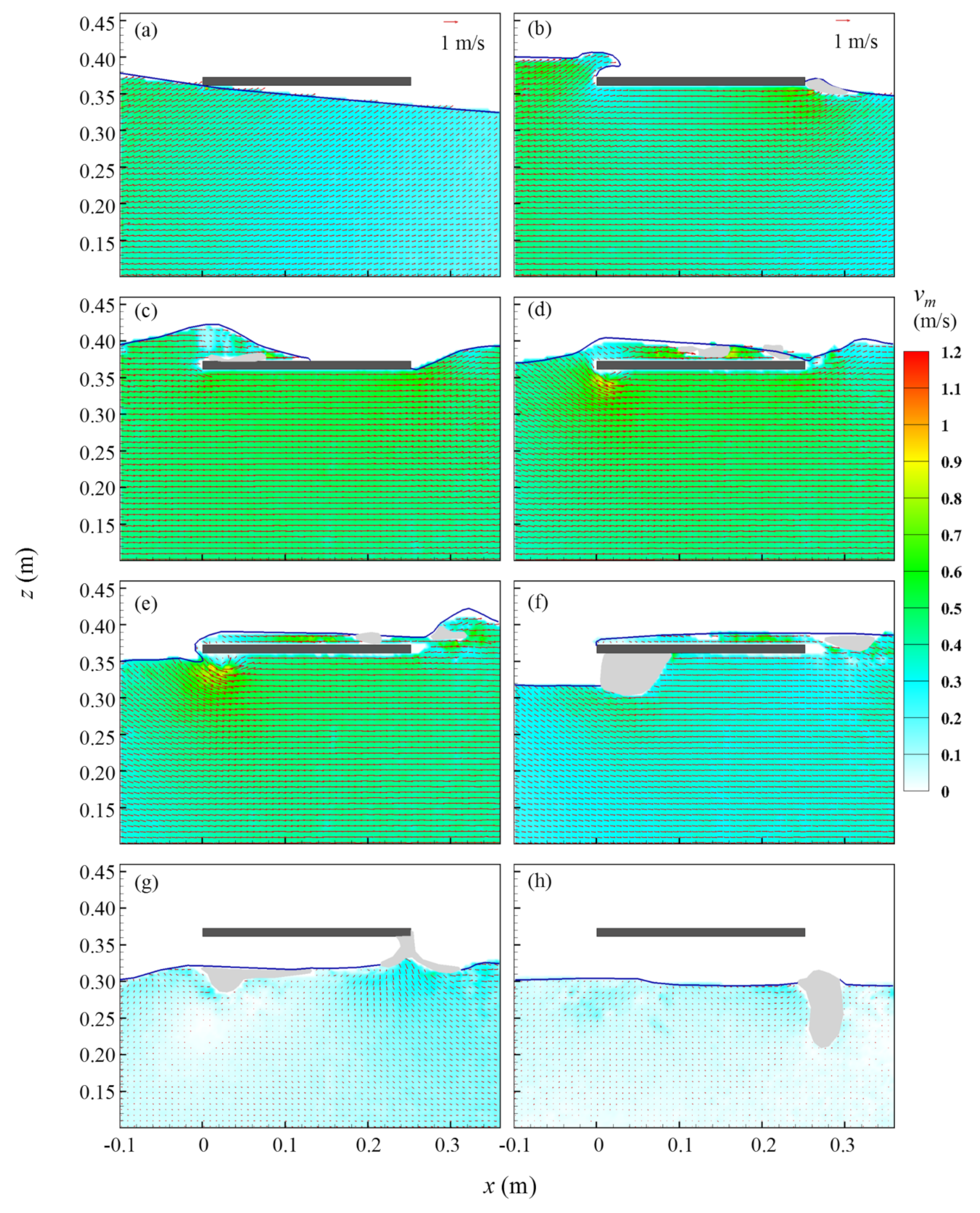
Figure 3 shows the velocity field around the plate obtained from the PIV measurement. The measurement range of the field is −0.10 m < x < 0.36 m and 0.10 m < z < 0.45 m measured from T = 0 to T = 1.92. The velocity fields consist of the velocity vectors and velocity–magnitude color maps. For clarity, only one–half velocity columns are plotted using a regularly spaced grid, and the light gray area is the location where aeration occurs. Before the wave impacts the plate, Figure 3a shows a purely developed solitary wave with no air bubbles entered. At this moment, the velocity is presented as relatively homogeneous, the horizontal velocity component is around 0.92 C0, which is higher than the vertical component with a value of around 0.30 C0. In this paper, C0 is the maximum flow velocity of the incident wave, as 0.68 m/s in this case. Figure 3b shows the velocity of splash–up along the front wall of the deck structure. Although the velocity is still horizontally dominated, there is a significant increase in vertical velocity. More specifically, the maximum horizontal and vertical velocity at this moment increases to the value of 1.28 C0 and 0.63 C0, respectively. After that, as the water tongue extends further forward, the horizontal velocity increases to 1.46 C0. Meanwhile, the maximum vertical velocity is 0.36 C0, significantly decreased compared to the previous period. This is mainly since the splashing tongue of water has finished its falling process. Right after the wave crests through the front of the plate, the dominating momentum changes immediately from upward speed to downward direction due to the phase change of the solitary wave. As shown in Figure 3d, an obvious flow separation phenomenon is presented at the front of the plate while a significant increase in vertical velocity occurs. The maximum horizontal and vertical velocity is around 1.57 C0 and 0.60 C0, respectively. At T = 0.74, the flow separation becomes more pronounced. As shown in Figure 3e, the maximum vertical velocity is around 0.81 C0, while the maximum horizontal velocity is around 1.47 C0. After T = 0.95, the green water is dominated by the separation phase from the plate, the measured velocity magnitude tends to reduce. More specifically, in Figure 3f–h, the maximum horizontal velocity decreases from 1.13 C0 to 0.43 C0, while the maximum vertical velocity decreases from 0.75 C0 to 0.32 C0.
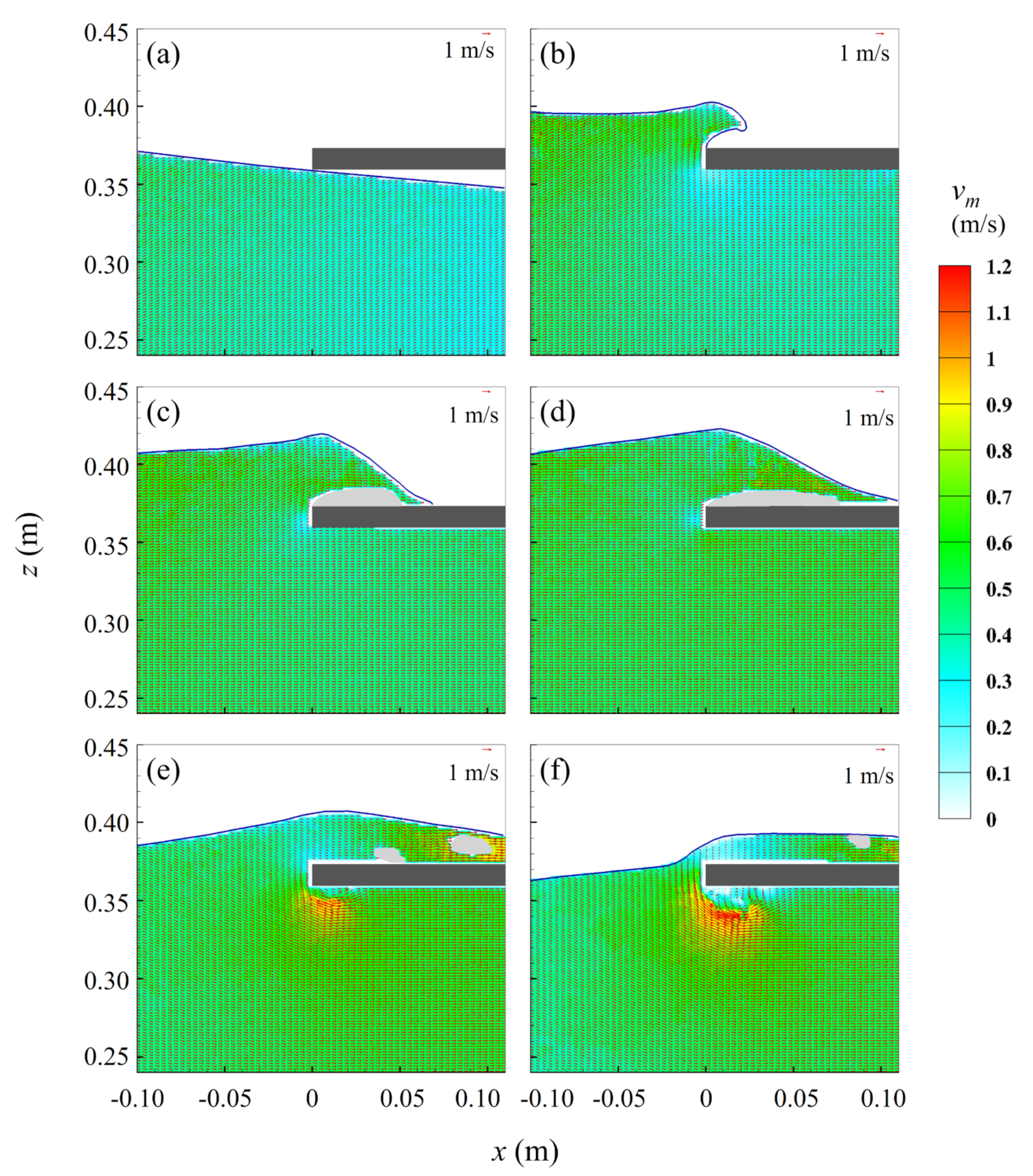
As it always relates to deck stability and vibration, velocity fields around the weather side of the plate are more concerned. In Figure 4, the detailed velocity fields near the front side of the structure are presented. A contour–clockwise vortex is observed at the bottom side of the plate in Figure 4f. Obvious energy accumulation can be seen at the edge of the vortex, such vortex structure was generated after T = 0.31, which is in the phase of wave crest has passed the front side. The vertical velocity changes from upward to downward, causing a flow separation phenomenon to occur on the bottom side. With the rotation of the vortex structure, large amounts of air are drawn into the water column at the edges of the vortex, exacerbating the separation of the green water from the plate.
In general, for the present experiment, the process of solitary wave impact on the plate can be categorized into the following three phases: (A) Green water tongue generation and run–up, (B) Green water overtopping along the plate, (C) Flow separation from the plate.
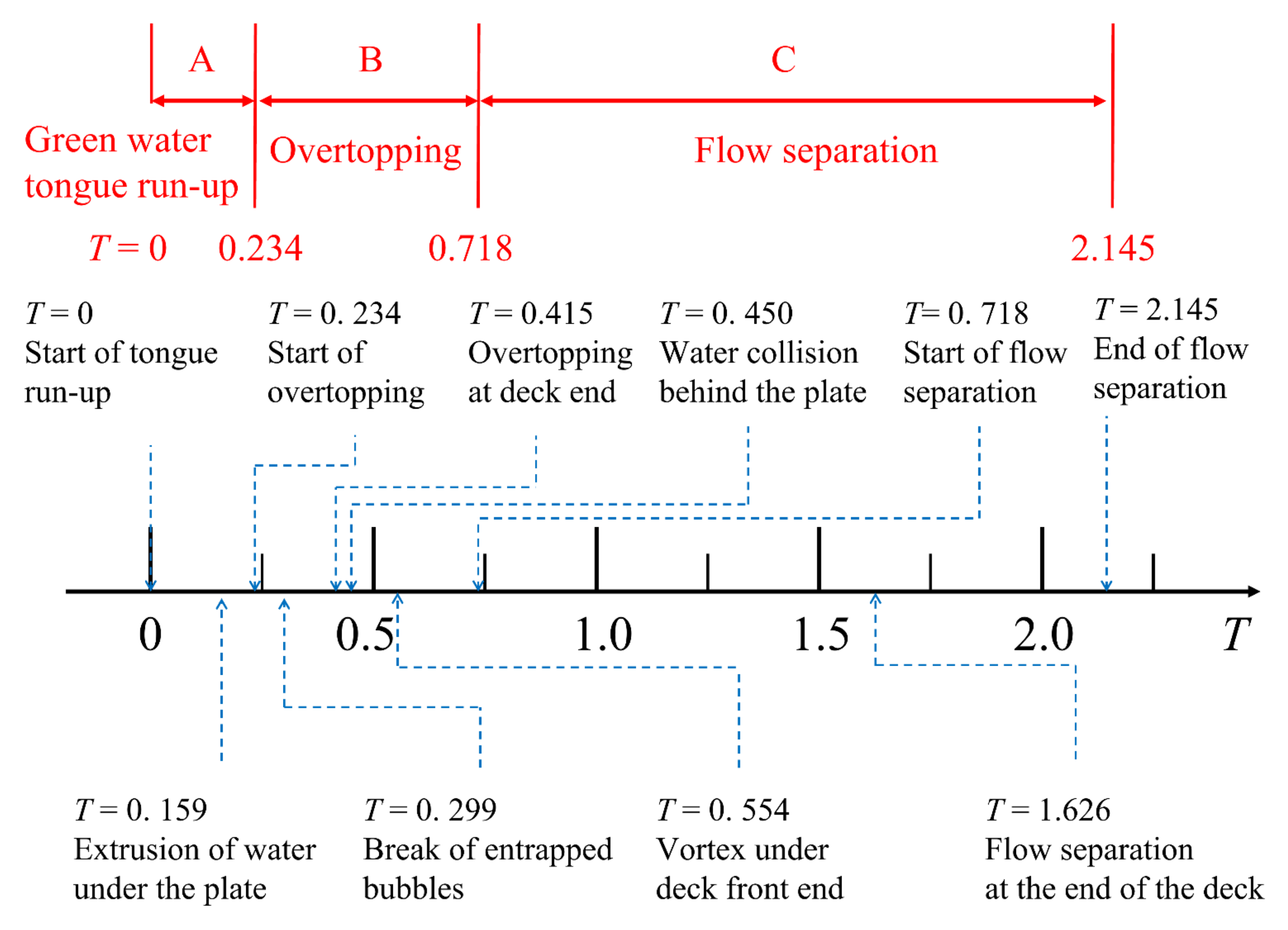
To illustrate the complete evolution of the flow field, the timeline of different stages is summarized in Figure 5. In the figure, the red arrows represent the period of different stages (A. Green water run–up, B. wave overtopping, C. Flow separation from the plate). The duration of each phase is T = 0.23, 0.48, and 1.43 separately. Meanwhile, the blue arrows represent the time nodes of typical flow characteristics. In Phase (A), the start of the green water tongue and the extrusion of water under the plate is included. Phase (B) includes the start of green water overtopping, the break of entrapped bubbles, wave overtopping at the end of the plate, water collision behind the plate, and vortex generation under the plate front end. In Phase (C), there are three typical features: the start of the flow separation, flow separation passing through the end of the plate, and the end of the whole green water process.
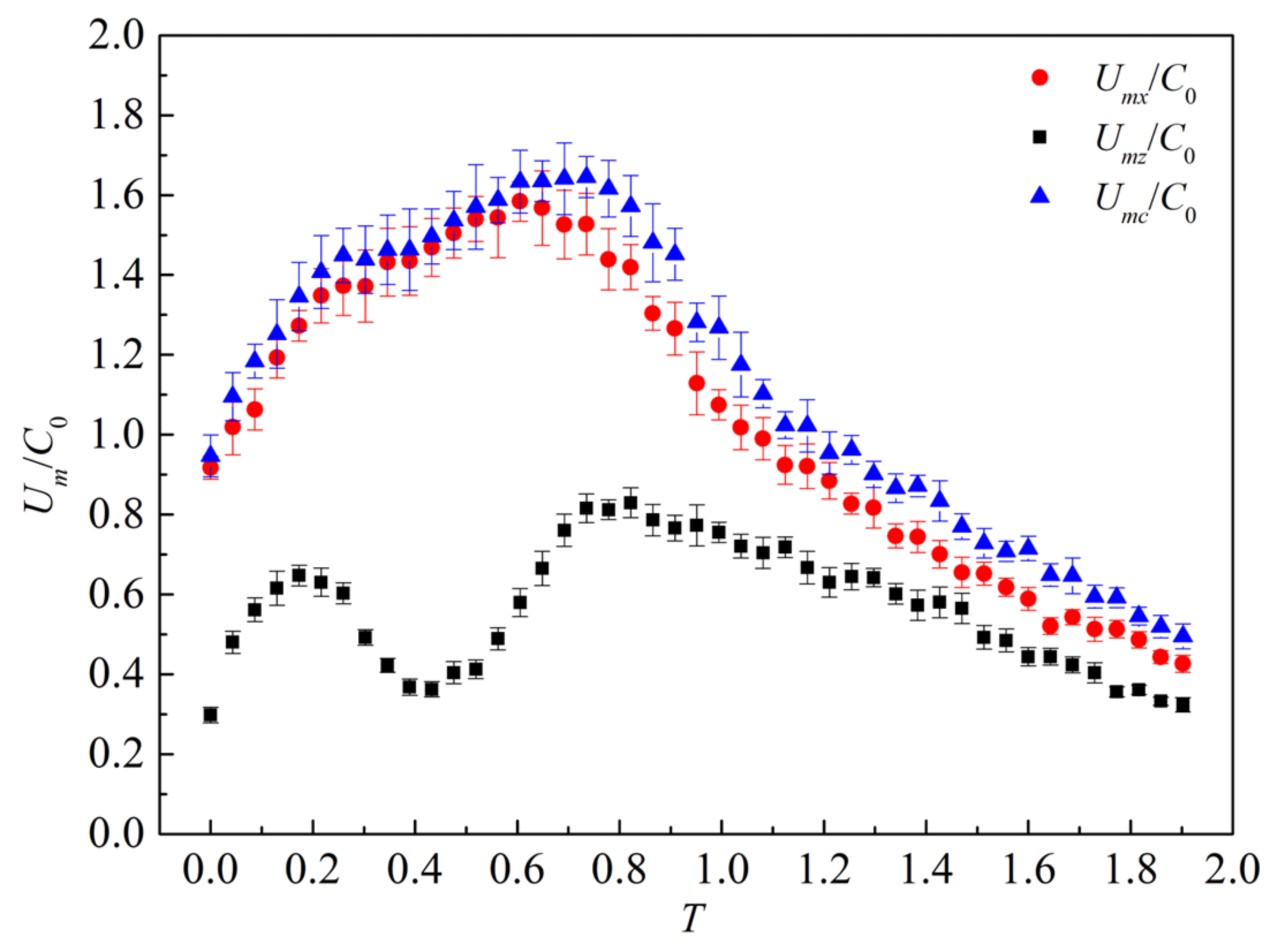
Based on the measured velocity, the maximum horizontal velocity Umx, maximum vertical velocity Umz, and the maximum velocity magnitude Umc is calculated. The time history of the maximum velocity is shown in Figure 6, where the vertical error bars represent the standard deviation of experimental repeated measurements. The velocity is normalized with C0, as C0 is defined in Equation (5) mentioned before as 0.68 m/s in this case. Generally, the green water process is presented to be dominated by the horizontal velocity. After the wavefront impact with the plate front side, the horizontal velocity increases significantly. At T = 0.61, the horizontal velocity increases to a maximum of 1.59 C0, and then the horizontal velocity starts to decrease. Different from the horizontal velocity, the trend of vertical velocity is more complex. With the wave tongue runup along the front side, the vertical velocity shows a rapid increase (0 < T < 0.18). Then, with the splashed tongue falling and attached to the top side of the plate, the maximum vertical velocity declines. After T = 0.42, flow separation starts to occur, causing the vertical velocity restarts to increase. With the incident wave passing forward, the vertical velocity decreases gradually. During this whole process, the maximum vertical velocity presents as 0.83 C0.
3.2. Effect of Wave Height and Structural Suspended Height
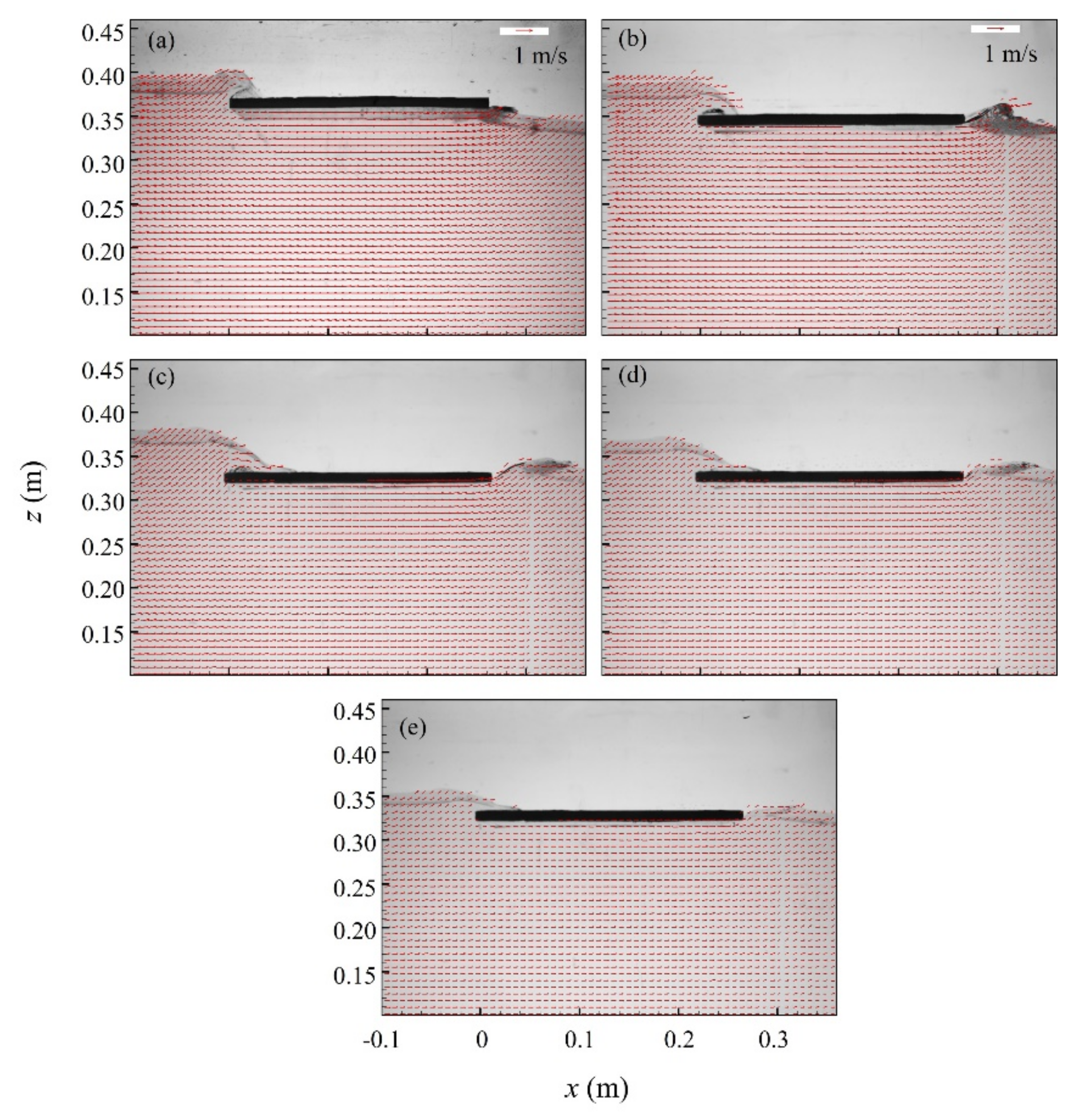
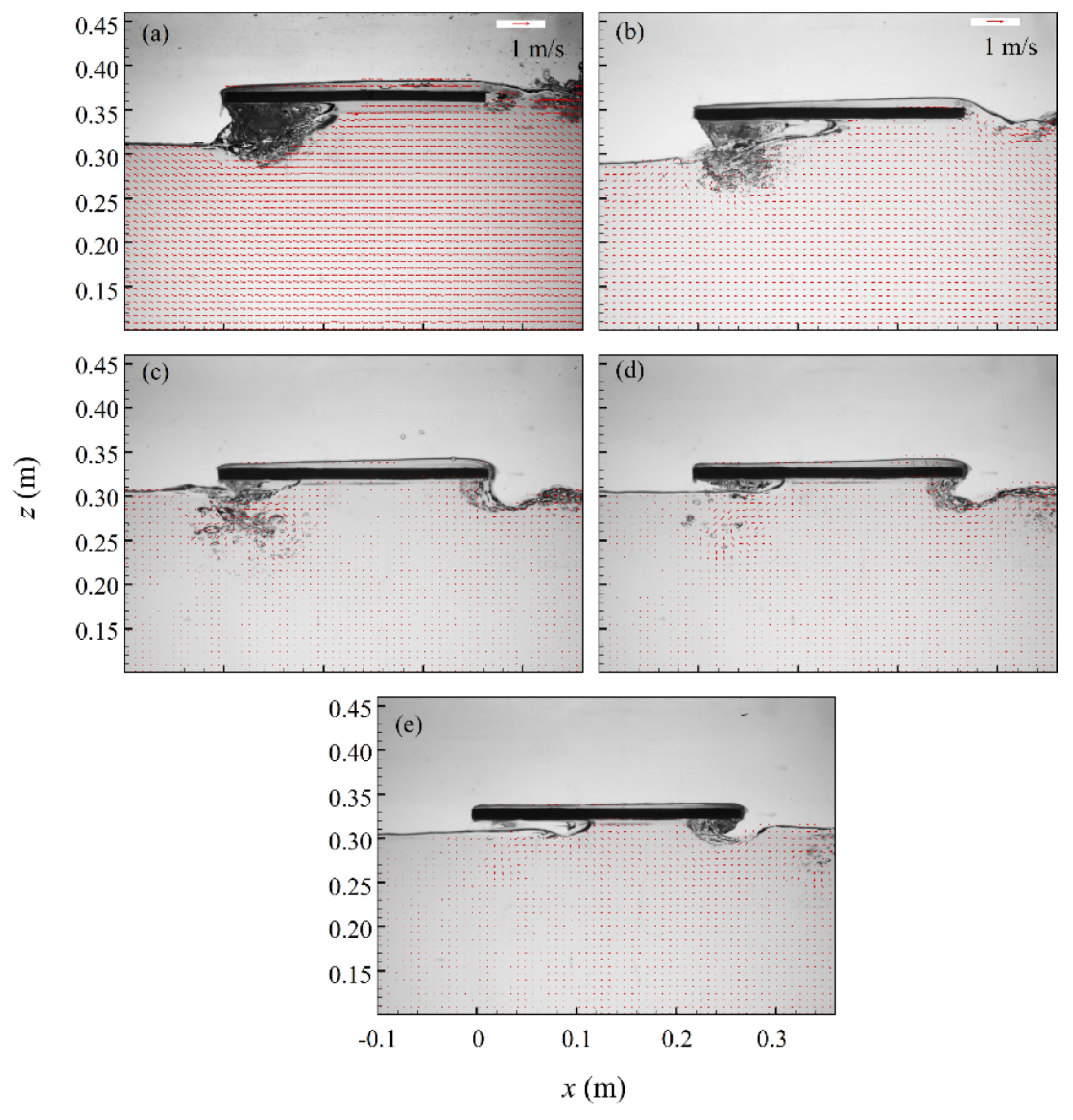
The detailed process of flow evolution for Case 1 was described above. In this section, we mainly analyze the effect of characteristic parameters (D/h and H/h) on the flow process. Figure 7, Figure 8 and Figure 9 present the velocity–field instants of different cases. Three instants T = 0.17, 0.69, and 1.03 are chosen as representative moments for Phase A, Phase B, and Phase C respectively. For the instant of T = 0.17, the velocity field of each case is shown in Figure 7. At this instant, within Phase A, the tongue of the jet flow above the plate is generated and dropped down, while the extrusion of water can be observed behind the plate. Case 1, Case 2, and Case 3 are carried out with the same incident wave, H/h = 10/30, but their structural heights are different as D/h = 6/30, 4/30, and 2/30. Meanwhile, the structural suspended height of Case 3, Case 4, and Case 5 are identical, but these cases are under different–scale incident waves. With fixed incident waves, the wave propagating velocity presents larger for lower structural height, as the water tongue rushes a farther distance for Case 3 (D = 2 cm). This effect can also be seen in the region behind the plate. The aerated volume extruded from the plate end is noticeably larger in the case of D/h = 2/30 and 4/30 than the one in the case of D/h = 6/30. For different incident wave heights, intuitively, lower wave causes slower global velocities and smaller aerated volume, by comparing the Figure 7c–e.
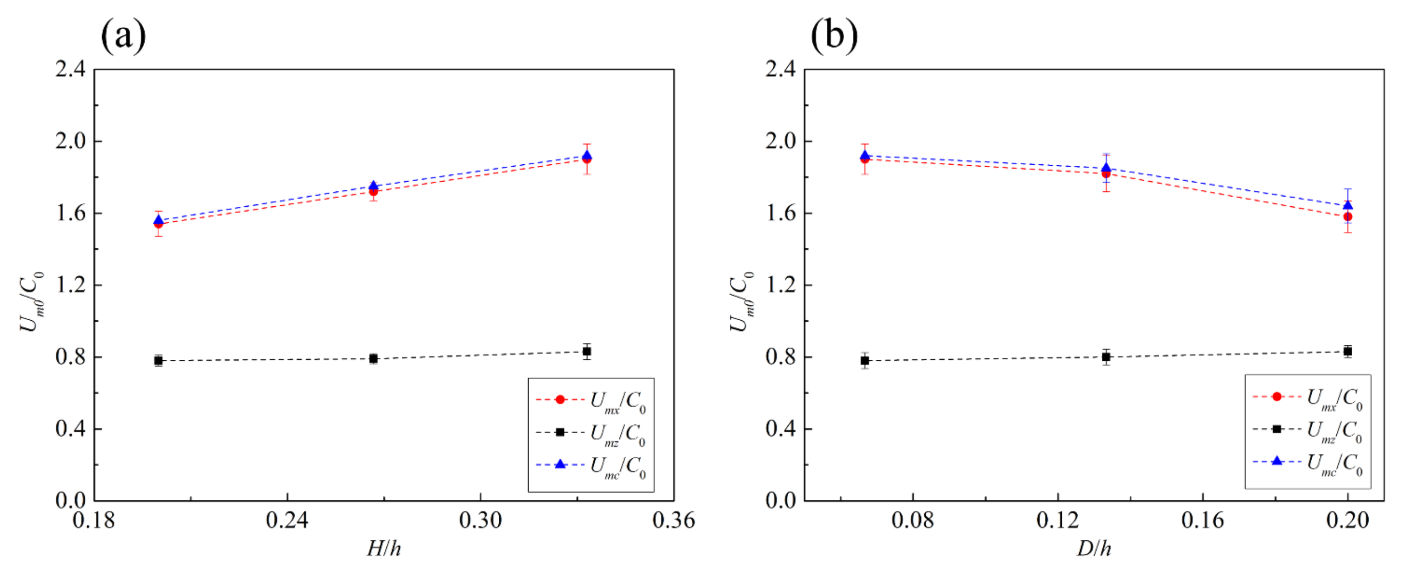
Furthermore, the maximum velocities of the five cases are presented in Figure 10. In the figure, the horizontal velocity, vertical velocity, and velocity magnitude are nondimensionalized by the C0 (incident–wave maximum velocity). Generally, the flow field is dominated by the horizontal velocity, as Umc presents little discrepancy with Umx. Note that the Umc is not the root mean square (RMS) of the Umx and Umz, as the maximum horizontal velocity and vertical velocity may not occur in the same position nor at the same time. Although the velocities are normalized by C0 which is dependent on the wave height, the Umx/C0 and Umc/C0 present incremental over the relative wave height, see Figure 10a. The Maximum Umx/C0 and Umc/C0 is 1.90 and 1.98, which are measured in the case of H/h = 10/30, D/h = 2/30. For the vertical velocity, Umz/C0, the maximum velocity is almost invariable with a constant around 0.8, only slight changes can be seen. For the cases of fixed incident–wave height (H/h = 10/30, Figure 10b), the ratio of maximum velocity magnitude to incident–wave velocity decreases over D/h, while the variation of Umz/C0 is still slight.
3.3. Comparing with the Green Water Model
It is well known that green water flow from the sides of a deck significantly resembles the behavior of dam–break flow [11,55]. According to Ryu, Chang and Mercier [29] and Chuang, et al. [56], the dam–break analogy of green water on fixed and floating structures in 2D flumes can be described through the Ritter solution [24] under certain circumstances. Based on their conclusions, the present study further examined whether the Ritter solution could be applied to green water caused by deck impingement events in the present condition.
For the dam–break problem, the conservation of mass and momentum is considered, which leads to the governing Saint Venant equations:
where x is the downstream distance from the dam, t is the time after dam failure, hd is the flow depth, is the horizontal velocity, g is the gravitational acceleration, S0 is the bottom slope, and Sf is the friction slope.
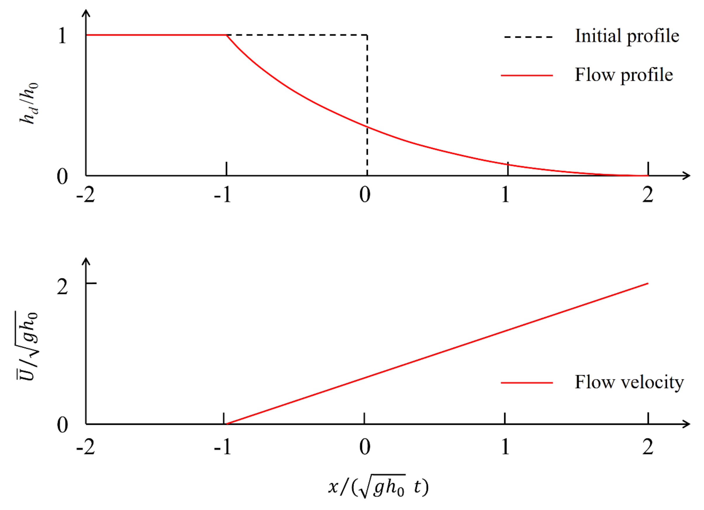
A mathematical solution for the dam–break flow was presented by Ritter [24] assuming that the flow is one–dimensional and has a uniform velocity distribution over the depth. There are two equations in Ritter’s solution, the first one describes the change of water depth regarding the distance, and the other is the distribution of the horizontal velocity:
where h0 is the initial water depth of the dam model.
Note that x/t is valid for , and the dam–break flow velocity is zero for . By examining Equation (8), it is evident that the velocity strongly depends on h0 and increases linearly concerning x. A diagrammatic sketch of Ritter’s solution is shown in Figure 11.
To compare the Ritter’s dam–break solution with the measured velocity field, it is necessary to match the variables at the same scale and coordinates between the dam–break flow and the green water flow. For dam–break flow, the x = 0 is the location of the dam. In our experiment, the leading edge of the plate in the green water measurements is set as the origin of the x coordinate, which is considered equivalent to the definition in the dam–break flow problem. Besides, for dam–break flow, the t = 0 is the instant of dam removal and the start of the green water process. In our experiment, as mentioned above, the t = 0 is defined as the instant when the solitary wave surface touches the leading end of the plate, in other words, the start of the green water. The wave momentum forces the wavefront to move forward onto the plate with the dominant momentum in the horizontal direction after t = 0. Having synchronized spatial coordinates and times, we can directly compare the dam–break solution with the green water measurements.
Based on the difference between the wave height and the suspended plate height, the initial water depth can be calculated as follows
where hdeck is the plate upper surface elevation from the still water level.
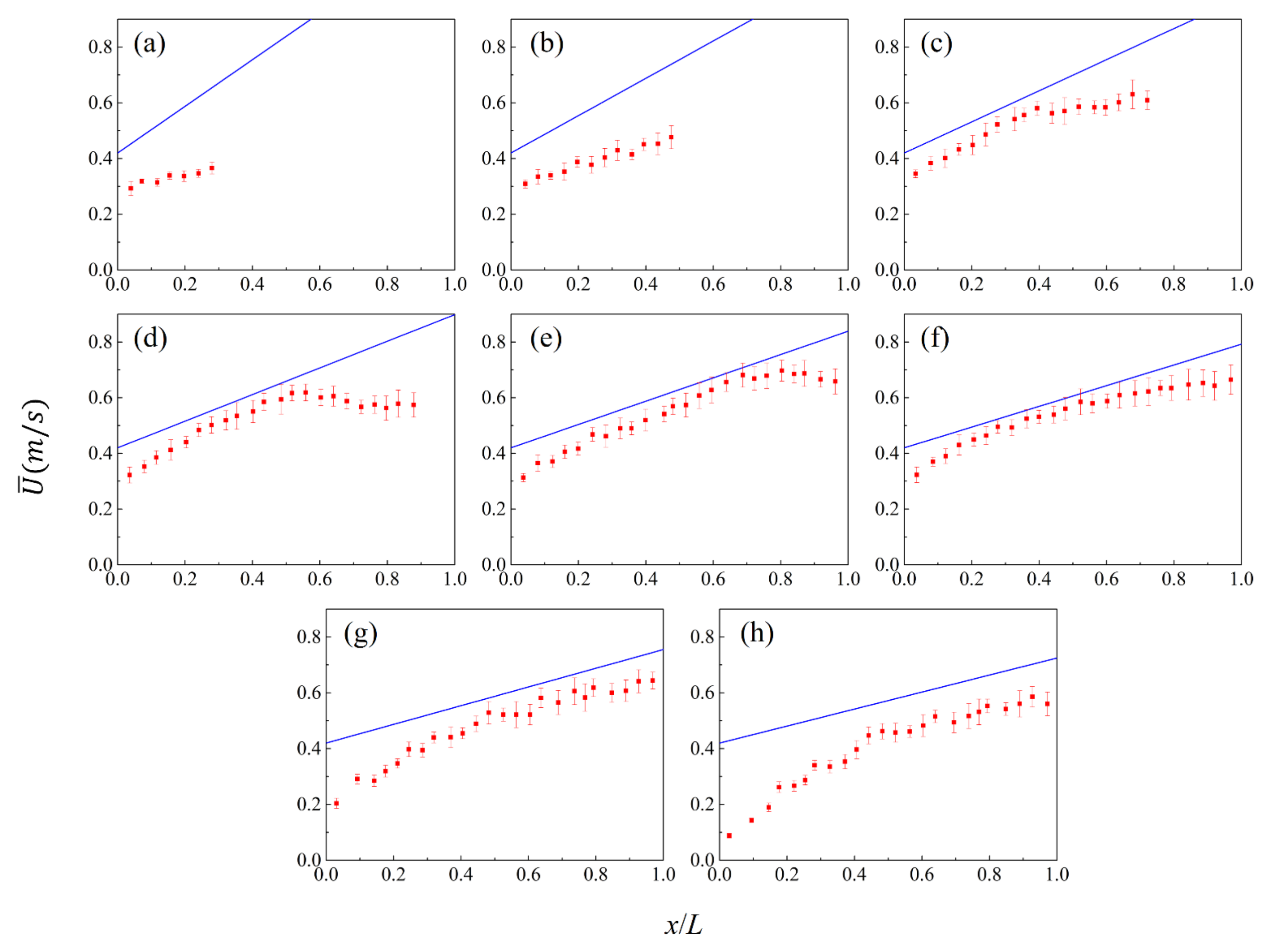
The comparisons for experimental data and Ritter’s solution for Case 1 are shown in Figure 12. Ritter’s solution is a one–dimensional velocity obtained from the dam–break flow solution. For comparison, the experimentally measured velocities were averaged in the depth direction. Note that in the figure the vertical error bars represent the standard deviation, and the ends of the red dot (corresponding to the maximum x values) indicate the farthest positions where the flow front propagates to.
Generally, as shown in Figure 12, Ritter’s solution is essentially a straight line while the green water flow measurements do not exactly show such a trend. Figure 12a corresponds to the moment of T = 0.35 when the green water tongue falls and attaches to the top side of the plate. The length of green water coverage is around 0.3 x/L. The measured horizontal velocity differs markedly from Ritter’s solution. At the tip of green water, Ritter’s value is around 74% larger than the measured velocity. While at the front end of the plate, such discrepancy is 55%. At T = 0.43, as shown in Figure 12b, the green water’s coverage comes to 0.52 x/L. In the same trend as before, the Ritter’s solution is much larger than the measured velocity. The maximum discrepancy of Ritter’s solution presents as 53%. With the wave propagating forward, the measured velocity distribution presents nonlinear against the distance, as shown in Figure 12c. However, based on linear theory, Ritter’s solution increases linearly. At T = 0.52, the Ritter’s value is 37% larger than the measured one. This difference becomes more pronounced at the location near the plate’s rear end. As the time increases, the value of the analytical solution becomes smaller and the difference with the measured value also decreases. As shown in Figure 12e, the analytical solution and experimental values are closer, except at the distal position of the plate. At this moment, the maximum discrepancy of Ritter’s solution is 21%. Furthermore, at T = 0.78, the Ritter’s solution fits the measured velocity better, while the maximum discrepancy is 12%. Then the depth–averaged velocity gradually deviates from the analytical solution, as the flow field is dominated by the flow separation (Phase C). At the front position of the plate, the speeds decrease significantly, presenting a large discrepancy with Ritter’s solution, especially at the more advanced instant of T = 0.95 (Figure 12h).
According to the above comparison, for case 1(D/h = 6/30, H/h = 10/30), the Ritter solution overestimated the depth–averaged velocity of green water flows in solitary wave conditions. In the initial stage of phase B (T ≤ 0.61), the discrepancy of Ritter solution with measured velocity is obvious. The measured velocity presents much smaller than the Ritter solution. However, in the later stage of phase B (T > 0.61), the Ritter solution agrees better with the measured depth–average velocity. In the stage of phase C (T > 0.87), the discrepancy of the Ritter solution becomes markedly again.
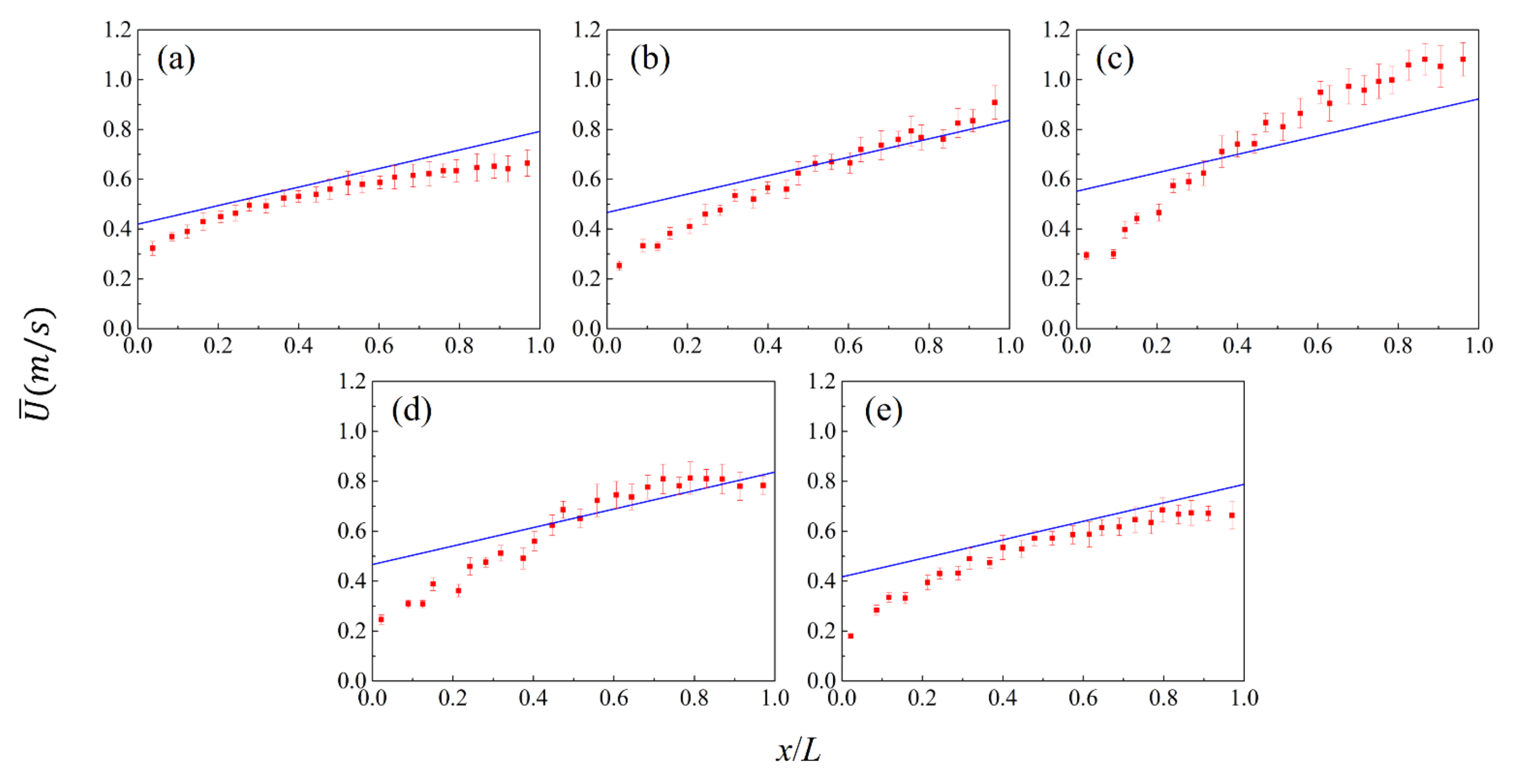
For all experimental cases, the comparisons of depth–averaged velocities (above the plate) and Ritter’s solution are shown in Figure 13, in which the measurement instance is T = 0.45. At this moment the experimental velocities are in good agreement with the dam–break solution. In the cases with the same incident waves (H/h = 10/30, Case 1, Case 2, and Case 3), the measured velocities increase along with the reduction of the model’s suspended height, presenting a trend beyond the Ritter’s solution, especially at the rear of the plate (x/L > 0.8). Besides, the velocities at the front of the plate have not shown an increasing trend. Furthermore, for the cases with fixed structural height (D/h = 2/30), the results are shown in Figure 13c–e. With smaller incident waves, the decrease of the velocities is obvious, mainly in the region of x/L ∈ (0.5, 1), where the cases of H/h = 10/30, 8/30 are beyond the dam–break solution. The velocities of case 5 (D/h = 2/30, H/h = 6/30) are slower than the ones of Ritter’s solution, but the trend of which is like that of case 1, possibly because they have the same submerged depth under the wave crest (H-hdeck = 3 cm).
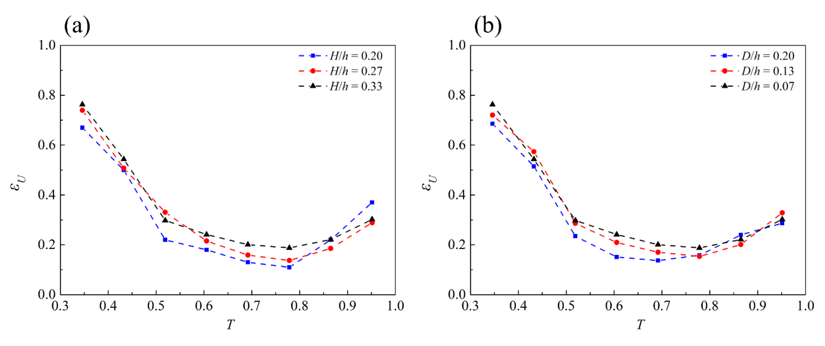
Furthermore, to quantify the predictive power of Ritter’s solutions for different cases. The deviation coefficients are calculated as , where is deviation coefficient; is measured depth–averaged velocity; is the corresponding Ritter’s solution; RMS means root mean square. The deviation coefficients in different cases with the same D/h or H/h are shown in Figure 14a,b. Generally, for all cases, the deviation coefficients decrease in the early stage and then present an increasing trend. The minimum of is in T = 0.6 to 0.9 range when the flow field is in the transition Phase from B to C. After the beginning of the separation, the fluid import is over, and velocities above the plate gradually decrease. This mechanism differs from the dam–break flow, causing the increase of . In Figure 14a, the cases with larger incident waves present larger deviation coefficients, the minimum of which is 0.11 as the case of H/h = 0.20. For the cases with the same incident waves, the minimum of is 0.13, presented in case 1 (D/h = 0.20). The results of minimum are consistent with the velocity distributions in Figure 13.
4. Conclusions
The present study experimentally investigates the 2–D kinematic properties of solitary waves’ impact on a suspended plate. The plate–type structure is rigid and fixed at 2 cm, 4 cm, and 6 cm above the water, as the water depth maintains at 30 cm throughout experiments. Solitary waves with heights ranging from 6 cm to 10 cm are generated to simulate the front bore of nearshore tsunami waves. The Particle Image Velocimetry (PIV) technique has been employed to measure the flow field around the plate. Besides, the experimental data are valuable as a benchmark problem for further numerical model refinement. The main conclusion of this study can be drawn as follows:
- (1)
- The flow evolution of green water can be categorized into the following three phases: (A) Green water tongue generation and run–up, (B) Green water overtopping along the plate, and (C) Flow separation from the plate. In Phase A, the wavefront contacts the plate at T = 0. At the front side of the plate, a green water tongue was generated and run up rapidly. Subsequently, the water tongue overturns and slaps the upper surface of the plate. Phase B includes the effects of the start of green water overtopping, the burst of entrapped bubbles, wave overtopping at the end of the plate, water collision behind the plate, and vortex generation under the plate front end. In Phase C, the flow separation starts at the front side of the plate and ends at the rear side of the plate;
- (2)
- Structural suspended height and incident wave size have different influences on the flow properties in each stage. Their evolutions present obvious similarities in general but several differences in detail. The increase in plate height will lead to a decrease in global velocities, less air entrapped in Phase B but a larger aerated area in Phase C. Besides, the increase in incident wave height can cause a significant increase in global velocities and more air involved in the water;
- (3)
- The maximum velocity around the plate was counted and normalized with C0 (the maximum flow speed of the incident wave). There is little difference between the velocity magnitude and the horizontal component, indicating the flow kinematics is dominated by the horizontal flow. The normalized maximum horizontal velocity increase with larger incident waves and decrease with higher suspended height, while the ratio of maximum vertical velocity to C0 is almost invariable with a constant around 0.8;
- (4)
- The Ritter’s dam–break flow solution for the prediction of green water flow in solitary wave conditions was validated. This solution agrees with the vertical–average horizontal velocities above the plate in the period of T ∈ (0.6, 0.9) when the flow field is in the transition stage from Phase B to Phase C. The rest of the time, the distribution of velocity does not conform to the description of Ritter’s solution. The minimum deviation coefficient throughout the present experiments appears in the case with the smallest submerged depth (under the wave crest, 3 cm).
Author Contributions
X.N.: investigation, data curation, writing—original draft preparation & visualization; Y.M.: Conceptualization, methodology, writing—review and editing & validation; G.D.: supervision, project administration & funding acquisition. All authors have read and agreed to the published version of the manuscript.
Funding
This research is supported financially by the National Nature Science Foundation of China (Grant No. 51720105010, 51979029) and the Fundamental Research Funds for the Central Universities (Grant No. DUT2019TB02).
Data Availability Statement
The data presented in this study are available on request from the author Xuyang Niu. Mail: [email protected].
Conflicts of Interest
The authors declare no conflict of interest.
References
- Hayatdavoodi, M.; Seiffert, B.; Ertekin, R.C. Experiments and computations of solitary-wave forces on a coastal-bridge deck. Part II: Deck with girders. Coast. Eng. 2014, 88, 210–228. [Google Scholar] [CrossRef]
- Maruyama, K.; Tanaka, Y.; Kosa, K.; Hosoda, A.; Mizutani, N.; Nakamura, T. Evaluation of tsunami force acted on bridges by Great East Japan Earthquake. In Proceedings of the Thirteenth East Asia–Pacific Conference on Structural Engineering and Construction (EASEC–13), Sapporo, Japan, 11–13 September 2013; 2013. Available online: https://hdl.handle.net/2115/54508 (accessed on 7 June 2022).
- Bredmose, H.; Peregrine, D.H.; Bullock, G.N. Violent breaking wave impacts. Part 2: Modelling the effect of air. J. Fluid Mech. 2009, 641, 389–430. [Google Scholar] [CrossRef]
- Silva, D.F.; Coutinho, A.L.; Esperanca, P.D.T. Green water loads on FPSOs exposed to beam and quartering seas, Part I: Experimental tests. Ocean Eng. 2017, 140, 419–433. [Google Scholar] [CrossRef]
- Greco, M.; Colicchio, G.; Faltinsen, O.M. Shipping of water on a two–dimensional structure. Part 2. J. Fluid Mech. 2007, 581, 371–399. [Google Scholar] [CrossRef]
- Bea, R.G.; Xu, T.; Stear, J.; Ramos, R. Wave forces on decks of offshore platforms. J. Waterw. Port Coast. Ocean Eng.-Asce 1999, 125, 136–144. [Google Scholar] [CrossRef]
- Rosetti, G.F.; Pinto, M.L.; de Mello, P.C.; Sampaio, C.M.; Simos, A.N.; Silva, D.F. CFD and experimental assessment of green water events on an FPSO hull section in beam waves. Mar. Struct. 2019, 65, 154–180. [Google Scholar] [CrossRef]
- Ma, Y.; Dong, G.; Perlin, M.; Ma, X.; Wang, G. Experimental investigation on the evolution of the modulation instability with dissipation. J. Fluid Mech. 2012, 711, 101–121. [Google Scholar] [CrossRef]
- Peregrine, D.H.; Thais, L. The effect of entrained air in violent water wave impacts. J. Fluid Mech. 1996, 325, 377–397. [Google Scholar] [CrossRef]
- Peregrine, D.H. Water−Wave Impact on Walls. Annu. Rev. Fluid Mech. 2003, 35, 23–43. [Google Scholar] [CrossRef]
- Stansby, P.K.; Chegini, A.; Barnes, T.C.D. The initial stages of dam–break flow. J. Fluid Mech. 1998, 374, 407–424. [Google Scholar] [CrossRef]
- Wu, Y.-T.; Liu, P.L.-F.; Hwang, K.-S.; Hwung, H.-H. Runup of Laboratory–Generated Breaking Solitary and Periodic Waves on a Uniform Slope. J. Waterw. Port Coast. Ocean Eng. 2018, 144. [Google Scholar] [CrossRef]
- Cox, D.T.; Scott, C.P. Exceedance probability for wave overtopping on a fixed deck. Ocean Eng. 2001, 28, 707–721. [Google Scholar] [CrossRef]
- Cox, D.T.; Ortega, J.A. Laboratory observations of green water overtopping a fixed deck. Ocean Eng. 2002, 29, 1827–1840. [Google Scholar] [CrossRef]
- Ryu, Y.; Chang, K.-A.; Mercier, R. Runup and green water velocities due to breaking wave impinging and overtopping. Exp. Fluids 2007, 43, 555–567. [Google Scholar] [CrossRef]
- Gómez-Gesteira, M.; Cerqueiro, D.; Crespo, C.; Dalrymple, R. Green water overtopping analyzed with a SPH model. Ocean Eng. 2005, 32, 223–238. [Google Scholar] [CrossRef]
- Shao, S.; Ji, C.; Graham, D.I.; Reeve, D.E.; James, P.W.; Chadwick, A.J. Simulation of wave overtopping by an incompressible SPH model. Coast. Eng. 2006, 53, 723–735. [Google Scholar] [CrossRef]
- Lu, H.; Yang, C.; Löhner, R. Numerical studies of green water impact on fixed and moving bodies. Int. J. Offshore Polar Eng. 2012, 22. Available online: https://onepetro.org/IJOPE/article-abstract/35604/Numerical-Studies-of-Green-Water-Impact-On-Fixed?redirectedFrom=fulltext (accessed on 7 June 2022).
- Qin, H.; Tang, W.; Hu, Z.; Guo, J. Structural response of deck structures on the green water event caused by freak waves. J. Fluids Struct. 2016, 68, 322–338. [Google Scholar] [CrossRef]
- Chang, K.-A.; Ariyarathne, K.; Mercier, R. Three–dimensional green water velocity on a model structure. Exp. Fluids 2011, 51, 327–345. [Google Scholar] [CrossRef]
- Chuang, W.-L.; Chang, K.-A.; Mercier, R. Kinematics and dynamics of green water on a fixed platform in a large wave basin in focusing wave and random wave conditions. Exp. Fluids 2018, 59, 100. [Google Scholar] [CrossRef]
- Nielsen, K.B.; Mayer, S. Numerical prediction of green water incidents. Ocean Eng. 2004, 31, 363–399. [Google Scholar] [CrossRef]
- Yan, B.; Bai, W.; Qian, L.; Ma, Z. Study on hydro-kinematic characteristics of green water over different fixed decks using immersed boundary method. Ocean Eng. 2018, 164, 74–86. [Google Scholar] [CrossRef]
- Ritter, A. Die fortpflanzung der wasserwellen. Z. Vere. Deutsch. Ing. 1892, 36, 947–954. [Google Scholar]
- Lauber, G.; Hager, W.H. Experiments to dambreak wave: Horizontal channel. J. Hydraul. Res. 1998, 36, 291–307. [Google Scholar] [CrossRef]
- Buchner, B. The impact of green water on FPSO design. In Proceedings of the Offshore Technology Conference, Richardson, TX, USA, 1–4 May 1995. [Google Scholar] [CrossRef]
- Stoker, J. Water Waves. In The Mathematical Theory with Applications; Interscience Publishers Inc.: New York, NY, USA, 1957. [Google Scholar]
- Yilmaz, O.; Incecik, A.; Han, J. Simulation of green water flow on deck using non–linear dam breaking theory. Ocean Eng. 2003, 30, 601–610. [Google Scholar] [CrossRef]
- Ryu, Y.; Chang, K.-A.; Mercier, R. Application of dam–break flow to green water prediction. Appl. Ocean Res. 2007, 29, 128–136. [Google Scholar] [CrossRef]
- Kleefsman, K.; Fekken, G.; Veldman, A.; Iwanowski, B.; Buchner, B. A Volume–of–Fluid based simulation method for wave impact problems. J. Comput. Phys. 2005, 206, 363–393. [Google Scholar] [CrossRef] [Green Version]
- Lee, H.-H.; Lim, H.-J.; Rhee, S.H. Experimental investigation of green water on deck for a CFD validation database. Ocean Eng. 2012, 42, 47–60. [Google Scholar] [CrossRef]
- Silva, D.F.; Esperança, P.T.; Coutinho, A.L. Green water loads on FPSOs exposed to beam and quartering seas, Part II: CFD simulations. Ocean Eng. 2017, 140, 434–452. [Google Scholar] [CrossRef]
- Khayyer, A.; Gotoh, H.; Shao, S. Enhanced predictions of wave impact pressure by improved incompressible SPH methods. Appl. Ocean Res. 2009, 31, 111–131. [Google Scholar] [CrossRef] [Green Version]
- Khojasteh, D.; Tavakoli, S.; Dashtimanesh, A.; Dolatshah, A.; Huang, L.; Glamore, W.; Sadat-Noori, M.; Iglesias, G. Numerical analysis of shipping water impacting a step structure. Ocean Eng. 2020, 209, 107517. [Google Scholar] [CrossRef]
- Lin, C.; Kao, M.-J.; Yang, J.; Raikar, R.V.; Yuan, J.-M.; Hsieh, S.-C. Particle acceleration and pressure gradient in a solitary wave traveling over a horizontal bed. AIP Adv. 2020, 10, 115210. [Google Scholar] [CrossRef]
- Lin, C.; Kao, M.-J.; Raikar, R.V.; Yuan, J.-M.; Yang, J.; Chuang, P.-Y.; Syu, J.-M.; Pan, W.-C. Novel similarities in the free-surface profiles and velocities of solitary waves traveling over a very steep beach. Phys. Fluids 2020, 32, 083601. [Google Scholar] [CrossRef]
- Qu, K.; Ren, X.; Kraatz, S. Numerical investigation of tsunami-like wave hydrodynamic characteristics and its comparison with solitary wave. Appl. Ocean Res. 2017, 63, 36–48. [Google Scholar] [CrossRef]
- Li, Y. Tsunamis: Non-Breaking and Breaking Solitary Wave Run-Up; California Institute of Technology: Pasadena, CA, USA, 2000. [Google Scholar]
- Yeh, H.; Liu, P.; Briggs, M.; Synolakis, C. Propagation and amplification of tsunamis at coastal boundaries. Nature 1994, 372, 353–355. [Google Scholar] [CrossRef]
- Wu, Y.-T.; Higuera, P.; Liu, P.L.-F. On the evolution and runup of a train of solitary waves on a uniform beach. Coast. Eng. 2021, 170, 104015. [Google Scholar] [CrossRef]
- Madsen, P.A.; Fuhrman, D.R.; Schäffer, H.A. On the solitary wave paradigm for tsunamis. J. Geophys. Res. Oceans 2008, 113. [Google Scholar] [CrossRef]
- Tadepalli, S.; Synolakis, C.E. Model for the Leading Waves of Tsunamis. Phys. Rev. Lett. 1996, 77, 2141–2144. [Google Scholar] [CrossRef]
- French, J.A. Wave Uplift Pressures on Horizontal Platforms; California Institute of Technology: Pasadena, CA, USA, 1969. [Google Scholar] [CrossRef]
- McPherson, R.L. Hurricane Induced Wave and Surge Forces on Bridge Decks; Texas A&M University: College Station, TX, USA, 2010. [Google Scholar]
- Lau, T.L.; Ohmachi, T.; Inoue, S.; Lukkunaprasit, P. Experimental and numerical modeling of tsunami force on bridge decks. In Tsunami–A Growing Disaster; IntechOpen: London, UK, 2011. [Google Scholar] [CrossRef] [Green Version]
- Seiffert, B.; Hayatdavoodi, M.; Ertekin, R.C. Experiments and computations of solitary-wave forces on a coastal-bridge deck. Part I: Flat Plate. Coast. Eng. 2014, 88, 194–209. [Google Scholar] [CrossRef]
- Qu, K.; Tang, H.S.; Agrawal, A.; Cai, Y. Hydrodynamic Effects of Solitary Waves Impinging on a Bridge Deck with Air Vents. J. Bridg. Eng. 2017, 22. [Google Scholar] [CrossRef]
- Chen, X.; Xu, G.; Lin, C.; Sun, H.; Zeng, X.; Chen, Z. A comparative study on lateral displacements of movable T-deck and Box-deck under solitary waves. Structures 2021, 34, 1614–1635. [Google Scholar] [CrossRef]
- Goring, D.G. Tsunamis—The Propagation of Long Waves onto a Shelf; California Institute of Technology: Pasadena, CA, USA, 1978; Available online: https://resolver.caltech.edu/CaltechKHR:KH-R-38 (accessed on 7 June 2022).
- Ma, Y.; Tai, B.; Dong, G.; Perlin, M. Experimental study of plunging solitary waves impacting a vertical slender cylinder. Ocean Eng. 2020, 202, 107191. [Google Scholar] [CrossRef]
- Korteweg, D.J.; de Vries, G. XLI. On the change of form of long waves advancing in a rectangular canal, and on a new type of long stationary waves. London, Edinburgh, Dublin Philos. Mag. J. Sci. 1895, 39, 422–443. [Google Scholar] [CrossRef]
- Boussinesq, J. Théorie des ondes et des remous qui se propagent le long d’un canal rectangulaire horizontal, en communiquant au liquide contenu dans ce canal des vitesses sensiblement pareilles de la surface au fond. J. Math. Pures Appl. 1872, 55–108. Available online: https://eudml.org/doc/234248 (accessed on 7 June 2022).
- Mei, C.C. The Applied Dynamics of Ocean Surface Waves; Massachusetts Institute of Technology; Advanced Series on Ocean Engineering; World Scientific Publishing Co. Pte. Ltd.: Singapore, 1989; Volume 1. [Google Scholar]
- Lee, J.-J.; Skjelbreia, J.E.; Raichlen, F. Measurement of Velocities in Solitary Waves. J. Waterw. Port Coast. Ocean Div. 1982, 108, 200–218. [Google Scholar] [CrossRef]
- Goda, K.; Miyamoto, T. A Study of Shipping Water Pressure on Deck by Two-Dimensional Ship Model Tests. J. Soc. Nav. Arch. Jpn. 1976, 1976, 16–22. [Google Scholar] [CrossRef]
- Chuang, W.-L.; Chang, K.-A.; Mercier, R. Impact pressure and void fraction due to plunging breaking wave impact on a 2D TLP structure. Exp. Fluids 2017, 58, 68. [Google Scholar] [CrossRef]
Figure 1.
General setup of present experiments: (a) sketch of the experimental setup; (b) definition of the temporal origin and the spatial coordinates; (c) measured surface profiles in the absence of the model; and (d) sketch map of the definition of the characteristic wave–passing period.
Figure 1.
General setup of present experiments: (a) sketch of the experimental setup; (b) definition of the temporal origin and the spatial coordinates; (c) measured surface profiles in the absence of the model; and (d) sketch map of the definition of the characteristic wave–passing period.

Figure 2.
Snapshots of aerated flow evolution around the plate of Case 1, D/h = 6/30, H/h = 10/30. T = (a) 0, (b) 0.17, (c) 0.42, (d) 0.62, (e) 0.74, (f) 0.95, (g) 1.45, (h) 1.92.
Figure 2.
Snapshots of aerated flow evolution around the plate of Case 1, D/h = 6/30, H/h = 10/30. T = (a) 0, (b) 0.17, (c) 0.42, (d) 0.62, (e) 0.74, (f) 0.95, (g) 1.45, (h) 1.92.

Figure 3.
Measured velocity fields around the plate on the side view of Case 1, D/h = 6/30, H/h = 10/30. T = (a) 0; (b) 0.17; (c) 0.42; (d) 0.62; (e) 0.74; (f) 0.95; (g) 1.45; and (h) 1.92.
Figure 3.
Measured velocity fields around the plate on the side view of Case 1, D/h = 6/30, H/h = 10/30. T = (a) 0; (b) 0.17; (c) 0.42; (d) 0.62; (e) 0.74; (f) 0.95; (g) 1.45; and (h) 1.92.

Figure 4.
Detailed weather–side velocity evolution around the plate of Case 1, D/h = 6/30, H/h = 10/30. T = (a) 0; (b) 0.17; (c) 0.31; (d) 0.42; (e) 0.62; and (f) 0.74.
Figure 4.
Detailed weather–side velocity evolution around the plate of Case 1, D/h = 6/30, H/h = 10/30. T = (a) 0; (b) 0.17; (c) 0.31; (d) 0.42; (e) 0.62; and (f) 0.74.

Figure 5.
Chronological sketches for green water evolution in the solitary wave (Case 1).

Figure 6.
Time history of maximum fluid velocities normalized by the wave velocity of Case 1, D/h = 6/30, H/h = 10/30, C0 = 0.68 m/s.
Figure 6.
Time history of maximum fluid velocities normalized by the wave velocity of Case 1, D/h = 6/30, H/h = 10/30, C0 = 0.68 m/s.

Figure 7.
Measured velocity fields around the plate of different cases at T = 0.17 (Phase A): (a) case 1, D/h = 6/30, H/h = 10/30; (b) case 2, D/h = 4/30, H/h = 10/30; (c) case 3, D/h = 2/30, H/h = 10/30; (d) case 4, D/h = 2/30, H/h = 8/30; and (e) case 5, D/h = 2/30, H/h = 6/30.
Figure 7.
Measured velocity fields around the plate of different cases at T = 0.17 (Phase A): (a) case 1, D/h = 6/30, H/h = 10/30; (b) case 2, D/h = 4/30, H/h = 10/30; (c) case 3, D/h = 2/30, H/h = 10/30; (d) case 4, D/h = 2/30, H/h = 8/30; and (e) case 5, D/h = 2/30, H/h = 6/30.

Figure 8.
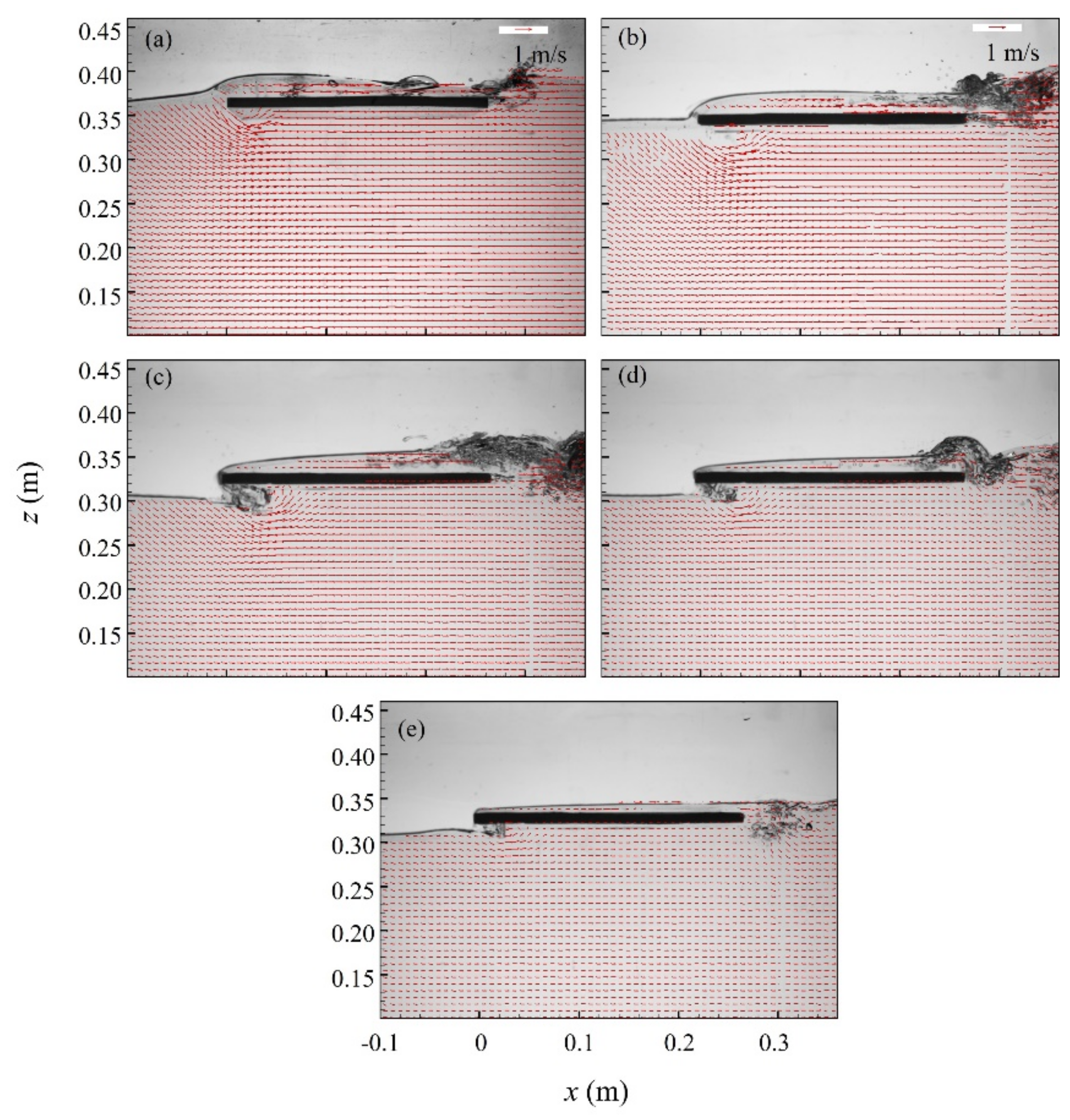
Same with Figure 7 for T = 0.69 (Phase B). (a) Case 1, D/h = 6/30, H/h = 10/30; (b) Case 2, D/h = 4/30, H/h = 10/30; (c) Case 3, D/h = 2/30, H/h = 10/30; (d) Case 4, D/h = 2/30, H/h = 8/30; (e) Case 5, D/h = 2/30, H/h = 6/30.
Figure 8.
Same with Figure 7 for T = 0.69 (Phase B). (a) Case 1, D/h = 6/30, H/h = 10/30; (b) Case 2, D/h = 4/30, H/h = 10/30; (c) Case 3, D/h = 2/30, H/h = 10/30; (d) Case 4, D/h = 2/30, H/h = 8/30; (e) Case 5, D/h = 2/30, H/h = 6/30.

Figure 9.
Same with Figure 7 for T = 1.03 (Phase C): (a) case 1, D/h = 6/30, H/h = 10/30; (b) case 2, D/h = 4/30, H/h = 10/30; (c) case 3, D/h = 2/30, H/h = 10/30; (d) case 4, D/h = 2/30, H/h = 8/30; and (e) case 5, D/h = 2/30, H/h = 6/30.
Figure 9.
Same with Figure 7 for T = 1.03 (Phase C): (a) case 1, D/h = 6/30, H/h = 10/30; (b) case 2, D/h = 4/30, H/h = 10/30; (c) case 3, D/h = 2/30, H/h = 10/30; (d) case 4, D/h = 2/30, H/h = 8/30; and (e) case 5, D/h = 2/30, H/h = 6/30.

Figure 10.
Maximum horizontal velocity, vertical velocity, and velocity magnitude of different cases: (a) case 3; case 4, and case 5, D/h = 2/30; and (b) case 1, case 2, and case 3, H/h = 10/30.
Figure 10.
Maximum horizontal velocity, vertical velocity, and velocity magnitude of different cases: (a) case 3; case 4, and case 5, D/h = 2/30; and (b) case 1, case 2, and case 3, H/h = 10/30.

Figure 11.
Diagrammatic sketch of Ritter’s solution.

Figure 12.
Comparisons of measured velocities and Ritter’s solution above the plate for case 1. Red dot: measured depth–averaged velocity, blue line: Ritter’s solution: T = (a) 0.35; (b) 0.43; (c) 0.52; (d) 0.61; (e) 0.69; (f) 0.78; (g) 0.87; and (h) 0.95.
Figure 12.
Comparisons of measured velocities and Ritter’s solution above the plate for case 1. Red dot: measured depth–averaged velocity, blue line: Ritter’s solution: T = (a) 0.35; (b) 0.43; (c) 0.52; (d) 0.61; (e) 0.69; (f) 0.78; (g) 0.87; and (h) 0.95.

Figure 13.
Comparisons of measured velocities and Ritter’s solution above the plate for T = 0.45. Red dot: measured depth–averaged velocity, blue line: Ritter’s solution: (a) case 1, D/h = 6/30, H/h = 10/30; (b) case 2, D/h = 4/30, H/h = 10/30; (c) case 3, D/h = 2/30, H/h = 10/30; (d) case 4, D/h = 2/30, H/h = 8/30; and (e) Case 5, D/h = 2/30, H/h = 6/30.

Figure 14.
Deviation coefficients between measured velocities and Ritter’s solutions: (a) case 3, case 4, and case 5, D/h = 2/30; and (b) case 1, case 2, and case 3, H/h = 10/30.
Figure 14.
Deviation coefficients between measured velocities and Ritter’s solutions: (a) case 3, case 4, and case 5, D/h = 2/30; and (b) case 1, case 2, and case 3, H/h = 10/30.


Table 1.
Experimental parameters.
| Case | Water Depth h (cm) | Plate Thickness (cm) | Plate Length L (cm) | Suspended Height D (cm) | Wave Height H (cm) | Max. Free Stream Velocity C0 (m/s) | Characteristic Period (s) |
|---|---|---|---|---|---|---|---|
| 1 | 30 | 1 | 25 | 6 | 10 | 0.683 | 0.578 |
| 2 | 4 | 10 | 0.683 | 0.752 | |||
| 3 | 2 | 10 | 0.683 | 1.001 | |||
| 4 | 2 | 8 | 0.513 | 1.045 | |||
| 5 | 2 | 6 | 0.366 | 1.079 |
Publisher’s Note: MDPI stays neutral with regard to jurisdictional claims in published maps and institutional affiliations. |
© 2022 by the authors. Licensee MDPI, Basel, Switzerland. This article is an open access article distributed under the terms and conditions of the Creative Commons Attribution (CC BY) license (https://creativecommons.org/licenses/by/4.0/).
Share and Cite
MDPI and ACS Style
Niu, X.; Ma, Y.; Dong, G. Laboratory Study on Flow Characteristics during Solitary Waves Interacting with a Suspended Horizontal Plate. Water 2022, 14, 2386. https://doi.org/10.3390/w14152386
AMA Style
Niu X, Ma Y, Dong G. Laboratory Study on Flow Characteristics during Solitary Waves Interacting with a Suspended Horizontal Plate. Water. 2022; 14(15):2386. https://doi.org/10.3390/w14152386
Chicago/Turabian StyleNiu, Xuyang, Yuxiang Ma, and Guohai Dong. 2022. "Laboratory Study on Flow Characteristics during Solitary Waves Interacting with a Suspended Horizontal Plate" Water 14, no. 15: 2386. https://doi.org/10.3390/w14152386
Note that from the first issue of 2016, this journal uses article numbers instead of page numbers. See further details here.