
Developing a Decision Support System for Regional Agricultural Nonpoint Salinity Pollution Management: Application to the San Joaquin River, California


1
School of Public Policy, University of California, Riverside, CA 92521, USA
2
HydroEcological Engineering Advanced Decision Support Research Group, Lawrence Berkeley National Laboratory, Berkeley, CA 94720, USA
*
Author to whom correspondence should be addressed.
Water 2022, 14(15), 2384; https://doi.org/10.3390/w14152384
Submission received: 24 April 2022
/
Revised: 1 July 2022
/
Accepted: 28 July 2022
/
Published: 1 August 2022
(This article belongs to the Special Issue Decision Support Tools for Water Quality Management)
Abstract
:Environmental problems and production losses associated with irrigated agriculture, such as salinity, degradation of receiving waters, such as rivers, and deep percolation of saline water to aquifers, highlight water-quality concerns that require a paradigm shift in resource-management policy. New tools are needed to assist environmental managers in developing sustainable solutions to these problems, given the nonpoint source nature of salt loads to surface water and groundwater from irrigated agriculture. Equity issues arise in distributing responsibility and costs to the generators of this source of pollution. This paper describes an alternative approach to salt regulation and control using the concept of “Real-Time Water Quality management”. The approach relies on a continually updateable WARMF (Watershed Analysis Risk Management Framework) forecasting model to provide daily estimates of salt load assimilative capacity in the San Joaquin River and assessments of compliance with salinity concentration objectives at key monitoring sites on the river. The results of the study showed that the policy combination of well-crafted river salinity objectives by the regulator and the application of an easy-to use and maintain decision support tool by stakeholders have succeeded in minimizing water quality (salinity) exceedances over a 20-year study period.
1. Introduction
Irrigated agriculture in semi-arid regions typically produces drainage return flows with high salinity content. Tanji and Kielen [1], review the conditions of low precipitation and high evaporation in semi-arid regions that lead to a high level of salinity in the drainage return flows. They provide examples from several locations such as the Nile Delta in Egypt, the Aral Sea Basin, and the San Joaquin Valley of California. An additional important region affected by salinity and the salinity pollution of water ways is the Murry Darling River Basin in Australia (Hart et al. [2]). The authors indicate that the clearance of deep-rooted native vegetation for the development of dryland agriculture and the development of irrigation systems in the basin have resulted in more water now entering the groundwater systems, resulting in mobilization of salt to the land surface and to rivers. In these examples, the return flows are discharged to water bodies (the Nile River, the Aral Sea, the San Joaquin River, and the Murry Darling River) that could benefit from regulation aimed to minimize negative externalities in the form of damage to crops and the environment. When these negative externalities exceed certain thresholds, the regulator can respond by assessing fines or other means of encouraging compliance with water quality objectives. We have seen different types of regulators, such as a river basin authority, in charge of managing the quantity and quality of water in the basin. A river basin authority could be a state or federal entity with the authority to impose fines or restrict water allocations in the case of nonpoint source pollution. Baccour et al. [3] model the case of the Ebro River Basin in Spain, where regulations to control nonpoint source pollution of nitrates from livestock production are addressed, among other policy interventions, by restriction of water supply, imposed by the Ebro Basin Authority. Quinn [4], compares the performance of real-time, basin-scale salinity regulation in the San Joaquin River in California with those of the Hunter River Basin authority, Australia.
Some numerical simulation models can be configured to act as decision support tools, which provide alerts of potential violations of water quality objectives, and can assist in the development of schemas for creating incentives or assessing fines to encourage compliance [5,6]. Obropta et al. [5] developed a model to address hot spots for a water quality trading program intended to implement the total maximum daily load (TMDL) for phosphorus in the Non-Tidal Passaic River Basin in New Jersey. Zhang et al. [6] develop a model-based decision support system for supporting water quality management under multiple uncertainties. Such tools can have the added benefit of allowing equitable imposition of proposed incentives or fines on those polluters who bear the primary responsibility for the load exceedances. Similar decision support tools have been developed in other sectors and contexts. Ioannou et al. [7] designed a DSS to help managers in the process of decision making, in handling areas that have been burnt by forest fires, by running hypothetical (what-if) scenarios in order to achieve the best form of intervention in fire-affected regions of Greece. Makropoulos et al. [8] demonstrate the development and use of a DSS to facilitate the selection of bundles of water-saving strategies and technologies to support the delivery of integrated, sustainable water management in the UK. Rose et al. [9] identify factors affecting the selection and use of decision support tools by farmers and farm advisers in the UK for agricultural planning purposes.
Our paper presents an approach using a regional framework that enhances the utility of existing modeling tools (Watershed Analysis Risk Management Framework—WARMF), which are currently in use by practitioners in the San Joaquin Valley (Systech Water Resources Inc. [10]), to make forecasts of the salt load assimilative capacity of a major river. The river receives salt loads from catchments in the form of irrigation return flows that often exceed the river’s salt load assimilative capacity. Uses of the modeling framework WARMF by practitioners are described by Quinn et al. [11], Fu et al. [12], and Quinn et al. [13], where WARMF features and performances are compared with other tools currently in use by practitioners.
The nonpoint source nature of agricultural salinity pollution poses a dual challenge for regulators by making it difficult to identify primary polluters, and to quantify pollution loads on a continuous basis. Not all drainage outlets can be monitored; therefore, calibrated simulation models play an important role in predicting pollutant loads under various permutations of hydrological and water quality inputs. Models allow alternative regulatory approaches, including schemes such as voluntary agreements and cap-and-trade in pollution permits to be evaluated, provided they can be adequately calibrated. Examples for such schemes are discussed and explained below [14,15,16,17,18,19,20,21,22,23].
Published literature on economic and regulatory aspects of nonpoint source pollution in irrigated agriculture highlights a variety of socio-political issues. These include the role of asymmetric information, value of information, effectiveness of policy interventions, and adoption of pollution reduction production practices. In an early work Griffin and Bromley [14], established a conceptual model for analyzing agricultural nonpoint pollution. An important aspect of pollution quantification is the representation of the biophysical processes linking production decisions to emission loads. Production decisions are reflected in the type and quantity of inputs in management practices and in local biophysical conditions.
An extension of the analysis in [14], was proposed in Shortle and Dunn [15], which included stochastic components in the pollution functions that arose from random natural processes as a means of addressing the lack of information about key biophysical processes. A review of various nonpoint source pollution control regulations (either incentives, taxes, or quotas) on inputs was also provided in Shortle and Dunn [15]. These are second-best interventions in the absence of direct measurements of polluter discharges. Shortle and Dunn [15], identified a reduction in the cost-effectiveness of these pollution control measures when applied uniformly across diverse agriculturally dominated subareas, which are heterogeneous in terms of water management practices and landscape characteristics, that can lead to different receiving water impact functions. To address such shortcomings, a cost-effective approach was developed by Shortle at al. [16] and was used to determine the best single-input tax policy for nonpoint source pollution in agriculture. The authors examined the question of reducing nitrate leaching from lettuce fields in California. Larson et al. [17] argue that under the certain circumstances applied, irrigation water can be the easiest single input to regulate since nitrate loading to groundwater is directly related to soil leaching rates. However, for other contaminants such as salinity, salt loads in subsurface drainage return flows may not be well correlated with surface water applications since most of the salt captured by the sub-surface drains may originate from deeper layers in the aquifer rather than from infiltrating water. Considerations of transaction costs and other political, legal, or informational constraints for dealing with nonpoint source pollution regulation were presented in Ribaudo et al. [18]. Such considerations could be applied to achieve specific environmental goals in a cost-effective manner. The authors discussed the economic characteristics of five instruments that could be used to reduce agricultural nonpoint source pollution (economic incentives, standards, education, liability, and research).
Several authors [9,10,11,12,13,14,15,16,17,18,19,20,21,22,23], considered regulation that had a spatial component in the presence of heterogeneity instead of regionally uniform instruments. In these works, authors demonstrated that spatially uniform policies resulted in economic efficiency losses and reduction in welfare. Kolstad [19], modeled a two-pollutant economy and showed that when marginal costs and benefits become steeper, the inefficiency associated with undifferentiated regulation increases. Wu and Babcock [20], demonstrate, among other things, that a uniform tax on polluter farmers may result in some farmers not using the chemical, and a uniform standard may have no effect on low-input land. Doole [21], finds that because of the disparity in the slopes of abatement–cost curves across dairy farms in New Zealand, a differentiated policy is more cost-effective at the levels of regulation required to achieve key societal goals for improved water quality. Doole and Pannell [22], find that due to variation in nitrate baseline emissions and the slopes of abatement–cost curves among polluting dairy farms renders a differentiated policy which is less costly than a uniform standard in the Waikato Region of New Zealand. Finally, the work by Esteban and Albiac [23], demonstrated and quantified the welfare loss from a spatially uniform regulatory policy to reduce salinity pollution and the efficiency gains from different policy measures based on the same spatial characteristics, applied in the Ebro River Basin of Spain.
Very few studies consider joint management of the nonpoint source pollution in a regional setting, using cooperative arrangements and trade, including trade-in water rights/quotas and trade-in pollution disposal permits in a regional setting. Several examples from actual cases exist. The Murray Darling Basin Authority [24], initiated a basin-wide agreement, a joint work program designed for setting salt disposal permits based on historical loads, including a revised cost-sharing formula and salinity credit allocation shares for Victoria, New South Wales, South Australia, and the Commonwealth [25]. In the Hunter Basin of New South Wales, Australia [25,26], a scheme of salt permit discharges has been put into work. The main idea of this scheme was to permit discharge of salt loads only when there was available salt load assimilative capacity in the Hunter River that drains the Hunter Basin. Quinn [4], reviews how salt load discharges to the river were scheduled by quantity, time, and location based on stakeholder need and calculations of salt load assimilative capacity using a simple spreadsheet mass–balance model.
Increasing use of high-salinity water as an irrigation source could be a serious problem. Yaron et al. [27] analyzed the economic potential to address such a problem by cooperative settlements in Israel and calculated income distribution schemes for three farms, using cooperative game theory (GT) algorithms. Work by Dinar et al. [28] also applied cooperative GT to the regional use of irrigation water under scarcity and salinity. Their model addressed inter-farm cooperation in water use for irrigation and determined the optimal water quantity and quality mix for each water user in the region.
Several additional works that represent various efforts and methods include Nicholson et al. [29] who conducted a comprehensive assessment of decision support tools used by farmers, advisors, water managers, and policy makers across the European Union as an aid to meeting the EU Common Agricultural Policy objectives and targets. Development and use of a GIS-based decision support framework was suggested by Chowdary et al. [30], integrating field scale models of nonpoint source pollution processes for assessment of nonpoint source pollution measures of groundwater-irrigated areas in India. A GIS was used to represent the spatial variation in input data over the project area and to produce a map that displayed the output from the recharge and nitrogen balance models. Different strategies for water and fertilizer were evaluated using this framework to foster long-term sustainability of productive agriculture in large irrigation projects.
The work by Quinn [4], which uses monitoring, modeling, and information dissemination for salt management in the Hunter River Basin in Australia, was compared to a more model-intensive approach deployed in the San Joaquin River Basin in California. Decision support systems for these river basins were developed to achieve environmental compliance and to sustain irrigated agriculture in an equitable and socially and politically acceptable manner. In both basins, web-based stakeholder information dissemination was a key for the achievement of a high level of stakeholder involvement and the formulation of effective decision support salinity management tools. The paper also compared the opportunities and constraints of governing salinity management in the two basins as well as the integrated use of monitoring, modeling, and information technology to achieve project objectives.
In the present paper, we provide a scalable water quality simulation model and decision support tool for a regional water quality (salinity) management problem that incorporates water/irrigation regions, each serving several individual farmers. The model operates at the subarea level where each subarea has distinct features that include political and hydrologic boundaries and which recognize different accesses to water supply and drainage resources. These subareas have been recognized by the State of California water regulatory agency with jurisdiction over the project area. We highlight the role of top-down regulations as well as market-based arrangements that might form a basis for cap and trade in pollution permits. We compare and discuss the physical as well as the welfare consequences of various policy interventions. The combination of monitoring system networks and decision support frameworks are scalable—hence, the final work product can be applied at the individual stakeholder level or aggregated at the water district level. Institutional and managerial components of the schema would need to be separately developed. Regional cooperation in the form of a market for tradeable salinity pollution permits [16], would be a significant outcome of a future study and one that is facilitated by the unique application of the simulation modeling tool.
The paper develops as follows: First, we present the analytical model aimed to evaluate the various options for pollution control at the subarea (regional) levels, responses of individual dischargers to introduced regulations, and the allocation of joint costs and benefits among the salt-discharging regions. Next, we introduce a proposed empirical framework to be applied to the San Joaquin River in California, given existing model resources in use by regulatory agencies. Then, we define a subset of seven subareas within the region as the basis for the empirical application aimed to test the analytical model. Finally, we evaluate the results to expand the method to incorporate future cooperative strategies.
2. Theoretical Model Building
2.1. Theoretical Perspective of the Analytical Model
We refer to a region that is composed of N subareas (n = 1, 2, …, N). Each subarea n could comprise water/irrigation districts that incorporate several agricultural producers regulated by individual water district mandates. Each subarea n includes Kn (kn = 1, 2, …, Kn) agricultural producers that are considered nonpoint source polluters of a given pollutant, or of a set of several pollutants (for simplicity we will refer to salinity as the pollutant in question). Each agricultural producer applies water on agricultural crops to produce market products. A byproduct in the form of agricultural pollution is the irrigation return flow that may contain a regulated water quality pollutant, which we will specify to be salinity.
Each of the k producers in the n-th subarea may have different factors affecting agricultural production conditions (natural and technical) that can lead to different cropping patterns, crop yields, net revenue, and the salt concentration and salt load of the return flow. We define a production function of agricultural yield and return flow for producer k as (for simplicity we drop the indexes k and n):
where Y is yield per acre of a given crop, W is water applied per acre, C is salinity level of applied water, T is irrigation technology used (expressed in integer values to indicate various irrigation technologies available to each agricultural grower within a designated subarea), Q is volume of return flow produced on that farm, S is the salt concentration of the return flows, and is a vector of all fixed effects related to the location of that producer. We will discuss later the first and second order conditions of the production function derivatives, namely the shape of these three components of the production function.
Given Equation (1), agricultural producers within a designated subarea maximize their net revenue under constraints imposed by both natural and regulatory conditions:
:
Additional constraints imposed on each agricultural producer within a designated subarea by subarea management, are summarized in (5), and discussed below
where for each agricultural producer within a designated subarea, p is the price per unit of crop, L is the area grown with that crop, w is the price of water, is the per-acre cost of the technology, is the total cultivable land of the agricultural producer, and is the water quota imposed by the subarea on the agricultural producer. Net revenue is defined as the revenue from crop sales minus the variable costs of production and payments of fees for exceedance of pollution load.
The solution to (2)–(5) provides for each agricultural grower within a designated subarea: the area under production with each crop selected; the total amount of water applied; the technology selected for each crop; the total profit; the total volume of return flow from the designated subarea; and the salt concentration of the return flow that can be used to compute drainage salt (mass) loads. While we may predict the volume Q and salt loading with associated S for each subarea, such information is not available to either the subarea management or to the federal regulator.
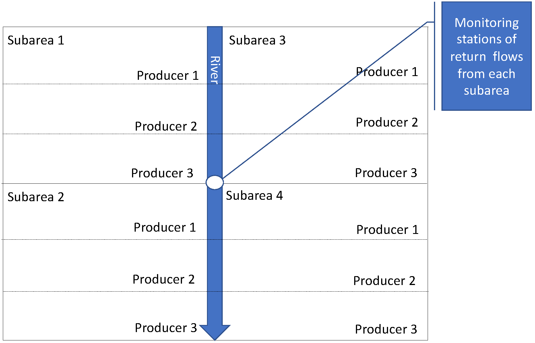
The subarea managers have access to monitoring data that provides the total volume of Q from all agricultural producers and its quality, S, that can be used to estimate salt loading. Salt loading is the factor each subarea manager is obligated not to exceed on a monthly and annual basis by the regulator, as defined within the Total Maximum Daily Load (TMDL) allocation for each subarea. TMDLs are the policy vehicles that are used by the US Environmental Protection Agency to limit nonpoint source pollution to levels that do not exceed the assimilative capacity of the receiving water body. TMDLs are keyed into water quality standards or objectives at a compliance monitoring station for the pollutant in the receiving water, and are designed to be protective. The agricultural non-point source pollutant management problem is a typical principal–agent problem under circumstances of asymmetry of information. Hence, we need to introduce several simplifying assumptions. We start by drawing (Figure 1) a schematic regional setting, using four agriculturally dominated subareas located on the valley floor, and a water body in the form of a river (describing the actual situation in the region that we will empirically analyze). The remaining three subareas are tributary river watersheds where water flow is controlled by upstream dams and reservoirs and whose operation is largely independent of agricultural drainage decision making.
2.2. Real-World Model Fitting
Water supply for the westside of the San Joaquin River Basin (SJRB) is provided by a water agency (e.g., United States Bureau of Reclamation) to the two westside subareas (Grasslands and the North-West Side subareas), according to water contracts negotiated between the water agency and individual water districts within each subarea. The individual water districts, in turn, allocate and distribute water supply according to agreements made with agricultural producers within each subarea. Water supply to subareas on the eastside of the SJRB derives largely from snowpack runoff from the Sierra Nevada Mountain Range, stored in downstream reservoirs along each major San Joaquin River (SJR) tributary. A state government water quality regulator (such as the California State Water Board), with the Regional Water Quality Control Board as enforcer, sets salt load objectives for the Basin in accordance with a Total Maximum Daily Load (TMDL) allocation developed by the Environmental Protection Agency for the basin. The load-based TMDL was further refined to develop subarea-level salt load allocations that take account of different water year hydrology. The conservative nature of the TMDL computation that utilizes the lowest 10% average low-flow condition resulted in allocations that were unattainable without major impact to the agricultural economy in each subarea. Hence, the initial TMDL allocations were replaced by concentration objectives, based on a 30-day running average electrical conductivity (EC), for the most downstream monitoring location on the SJR, Vernalis. A concentration objective allows agricultural producers and other salinity dischargers to utilize more of the available salt load assimilative capacity in the SJR. This initial compliance-monitoring objective has been supplemented with two additional upstream salinity objectives, ostensibly to protect the water quality of agricultural diversions made by westside agricultural producers. These additional salinity objectives are set at 1550 uS/cm year-round, as opposed to the 1000 uS/cm non-irrigation season, and 700 uS/cm objective set at Vernalis. The regulator suggested a number of approaches by which the original salinity load allocations, under the TMDL, might form the basis for salt load reduction strategies or cost allocation in situations where these various salt load objectives were violated.
The salinity load (mass of salt from all producers which is calculated by summing the product of drainage volume and salt concentration from each producer) produced on subarea n is the result of the return flows (drainage) from the agricultural activity of all producers, such that . There is no practical way that the regulator could equitably assign salt pollution levels to the individual agricultural producers or enforce this regulation at a reasonable cost to individual agricultural producers. Therefore, the regulator has chosen to allow stakeholders to internally govern the strategies to attain and abide by river EC objectives, while encouraging stakeholders to consider the subarea as the organizing entity for stakeholder action. Stakeholder compliance is monitored by the Regional Board using data supplied by state and federal water agencies.
To maintain compliance the agricultural producers can dynamically allocate salt loads to each subarea given that available salt load assimilative capacity at each compliance station is the product of the total assimilative capacity (defined by the current flow multiplied by the EC objective) and the current salt load in the river.
The monthly salt load cap can be calculated for each subarea individually based on the calculated TMDL allocations and the current salt loading to the river from each subarea (measured in terms of tons of salt: SL = d [salt concentration, S; volume, Q]), where SL is salt load (In the San Joaquin River the current TMDL criterion is a 30-day running average salt concentration that is multiplied by a monthly design flow to determine allowable salt loading). Using this stakeholder-maintained salinity load cap approach subareas would pay a fine (F) to the regulator, which could be a price per unit of salt load above the cap or some other equitable formula for dividing the fine amongst stakeholders. F can be specific to each subarea or similar for all subareas (see [23], for critique on uniform tax). F is then equitably distributed according to some formula (by land area, drainage volume, incremental salt load etc.) among all Kn agricultural producers in the different subareas (or by water user associations/districts in each subarea). We assume, for simplicity, that since we have a non-point source salinity management problem where the exact source of salt is not known, the most straight-forward and cost-effective initial approach to distribute F is to divide it equally per acre of land in production, or per acre–foot of irrigation water supply delivered. These initial approaches ignore the fact that some crops are associated with higher drainage return flow volumes and that subsurface drainage return flow salt loads may be poorly correlated with irrigation applications. Alternative allocation formulas may be relevant and will be considered in the empirical model. We assume that the (hypothetical) subarea manager (While there is no actual subarea manager, it is assumed that the model allocations are respected by the individual farmers and other decision makers at the water district level) has the authority or power to impose these allocations of river salt load assimilative capacity. We also do not want to set an optimal level for F, but rather take F as given in the empirical analysis. We will use several levels of F in a sensitivity analysis to evaluate the effect of F on the behavior of the agricultural decisionmakers at the subarea level.
An additional consideration is in the temporal administration of fines and fee schedules, which has a bearing on the design of a decision support system to aid the subarea manager to orchestrates stakeholder responses to potential violations of the river salinity objectives. An approach that attempts to respond to potential exceedance of salt load assimilative capacity at each compliance site in real-time would require model simulation tools that ran on a monthly timestep at a minimum. An optimization model would choose between available salt load reduction strategies, purchase of available water supply for dilution purposes, or payment of fines each month. Alternatively, accounting could be postponed until the end of each year and fines imposed retroactively. The latter strategy would rely on uncertainty and the fear of a potential exceedance to motivate compliance. However, the decision tool needed to support this strategy could be simplified to operate on an annual timestep.
2.3. Individual Responses to Water Quality Regulations
We expect that each stakeholder within each subarea will respond to F, depending on the level of F and the conditions (cropping patterns, physical conditions such as soil properties, etc.) in that subarea. In the empirical application, we will look at the effects of surface water and irrigation land and water limits and fees, as these are the main forms of regulation that can affect salinity load in the case of a nonpoint source pollution. In future empirical applications, we propose limits on the output of the model, specifically the salinity loading. Here, we outline the full analytical model.
Given F, each subarea faces the following two options:
- (a)
- Maintain the current (status quo) level of salt loading if F the cost of abatement. The cost of abatement could include changing the crop mix and/or land use changes (e.g., fallowing land) (Changes in land use (crop mix or fallowed land) is an important component to maximize revenue and obtain maximum resource use efficiency. In the empirical model, changes in land use is incorporated at a later stage in the model development process), surface and/or subsurface drainage reuse, investing in more efficient irrigation technology, changing irrigation scheduling, and other options.
- (b)
- Abate to a level of allowable salt loading than the cap. Each subarea will require abatement activities (detailed below) to the point where the marginal abatement cost equals F.
We consider the abatement in (a) and (b) to be “individual responses” to the salinity management regulation. That is, each subarea acts on its own responses, given its resources and local conditions (In the empirical application section, we also consider some of the individual responses, such as restrictions on water quotas, restrictions on cropping patterns, land fallowing, and investment in water-conserving irrigation technologies, as regulatory-imposed policies).
Each subarea is characterized by an aggregate revenue function (of all agricultural producers within each water district) minus fines on excess salt loading and minus abatement cost, such that
where is a fine on excess salt loads, is pollution fine per unit of excess salt load, is salt load, is abatement cost, and is a set of abatement options, such as changing cropping patterns, fallowing land, adopting more efficient irrigation technologies, and investing in monitoring drainage quantity and quality. Each subarea can select one of these abatement options or a subset of the abatement options.
2.4. Allocation of Joint Costs and Benefits in the Case of Individual Responses
In both individual and cooperative responses, we estimate the subarea net benefits as revenues minus variable operational costs and incremental costs. The incremental costs include costs associated with activities that polluters introduce to the agricultural production process in response to the regulatory objectives or constraints on input use imposed by the regulator for each subarea. In the case of a fine imposed on the entire region for exceeding the pollution EC objective, the subarea level of fine is allocated, based on several allocation principles, and the subarea amount of fine, , is added to the incremental costs. In the case of cooperation among the subareas; we estimate first the regional net benefits to the entire region. The value of the regional benefits is obtained by running a regional optimization model, coined ‘a social planner’ model, which maximizes the entire regional welfare rather than looking at welfare of each subarea individually.
Economic theory [31], suggests that a social planner allocating regional benefits or costs among the agents involved maximizes the joint welfare of the region, subject to physical and institutional constraints relevant to the situation under study. Under a social planner optimization, the region is seen as one unit without political borders. An optimal social planner allocation is considered as first best and serves as reference (benchmark) to which other allocation schemes are compared. Deviations from the social planner outcomes represent inefficiency (welfare loss) of the alternative allocations.
Once a regional social planner allocation solution has been found, the regional gains (either welfare benefits or savings of joint costs—such as regulatory fines) must be distributed among the regional parties. We will consider a couple of schemes for the allocation of the joint benefits or the costs of pollution control, or regulatory fines, among resource management regions, namely, the subareas (and the individual farmers in each subarea). For example, allocation of benefits or fines could be based on annual drainage flows or based on irrigated area. The likelihood of subareas forming stable coalitions aimed to reduce salt loads can be measured by comparing the empirical attributes of the standard allocation schemes with game theoretic allocation schemes whose acceptability and stability can be measured. We introduced several allocation schemes, based on the subarea’s contribution of pollution load and consistent with the strategy described previously [32].
2.4.1. Allocation of Regulatory Fines Based on Surface Water Applied
This allocation scheme simply suggests that each polluter (subarea) will be charged in proportion to the volume of surface water applied on that subarea. Therefore, the cost to subarea j is
where is the regulatory fine allocated to subarea j; F is total regional regulatory fine. This scheme allocates all the regulatory fine among all N subareas. is the volume of surface water applied for irrigation in subarea j (a summation over all irrigated area). The disadvantage of this regulatory method is that it does not target those stakeholders who physically discharge to the SJR and not take into account the significant reuse that occurs in some areas that helps to curtail salt loading to the river. It is a blunt policy instrument that is nonetheless relatively easy to administer.
2.4.2. Allocation of Regulatory Fines Based on Total Irrigation Water Applied
This allocation scheme simply suggests that each polluter (subarea) will be charged in proportion to the total volume of water applied (surface water + groundwater + recycled wastewater) on that subarea. Therefore, the cost to subarea j is
The drawbacks to this policy are the same as those of the prior policy, although, it does account for groundwater use that can add significant salt to the total salt discharged from each region, since the EC of groundwater is typically more than double that of applied surface water on the westside of the Valley, and more than four times the average EC of eastside water applications.
2.4.3. Allocation of Regulatory Fines Based on Salt Load Generation
The allocation scheme in (11) simply suggests that each polluter (subarea) will be charged in proportion to the amount of salt load it generates. Therefore, the cost to subarea j is
where is the quantity of salt load generated by subarea j.
This policy is the most equitable but also the most difficult to administer since current monitoring and modeling is insufficient to accurately measure or estimate the salt load export from each subarea. Current models are not capable of recognizing the amount off drainage reuse within each subarea.
2.4.4. Allocation of Regulatory Fines Based on Cultivated Area
The allocation based on cultivated area is built on a similar rule as in Equation (12), except that is cultivated land and not disposed drainage.
where is the cultivated land area in subregion j.
3. Model Testing
3.1. Application to Water Quality Issues in the San Joaquin River
Salinity loads to the San Joaquin River (SJR), the receiving water body for agricultural drainage in the San Joaquin Basin, are regulated by the State of California through the Central Valley Regional (Water Quality Control) Board. A TMDL was developed that set load limits for each subarea [33,34]. The TMDL for each of the seven subareas (Figure 2) was largely based on basin hydrography, and existing water district and jurisdictional boundaries. Four of these subareas (Northwest Side, East Valley Floor, Grasslands, and San Joaquin River Above Salt Slough) are located on the valley floor, and drainage from these subareas is dominated by agricultural and managed wetland decision-makers. The other three subareas are watersheds serving three major east-side tributaries to the SJR, namely the Stanislaus, Tuolumne, and Merced rivers. Given the institutional history and management functions within the basin, these seven subareas are the most logical management units and any possible future trade in salinity load permits would initially occur between these entities.
The load allocations under the TMDL ended up being overly restrictive, following the typical TMDL development methodology and would have resulted in potential annual fines in the order of USD 300,000 per subarea based on a 9-year average of salt loads. Load allocations were based on a design flow hydrology representing the lowest 10% of monthly flows. An additional safety factor was applied to the allowable monthly salt loads which further reduced stakeholder ability to meet objectives. The Regional Board adopted a real-time concentration-based schema to substitute for the TMDL salt load based approach which allowed greater use of the river’s assimilative capacity. Salinity management in the San Joaquin River Basin is complex, involving agricultural, wetlands, and municipal stakeholders within the basin. Being cognizant of this complexity and the difficulty of building coalitions among entities that had little history of working cooperatively, the Regional Water Board named the alternative approach to TMDL implementation “real-time salinity management”. The current Basin Water Quality Control Plan for the San Joaquin Basin lays out the general requirements for a Board-approved Real-Time Salinity Management Program:
- The program is a basin-wide program requiring all stakeholders discharging to the SJR to be signatories and active participants.
- Real-time monitoring networks should be developed and maintained to allow the estimation of net salt loading to the San Joaquin River and residual salt load assimilative capacity at the Vernalis compliance monitoring station.
- Provision should be made to allow for free and easy sharing of real-time flow and EC data that will be the basis for salt load assimilative capacity estimation.
- A decision support tool or simulation model should be developed to allow reliable forecasting of salt load assimilative capacity to give stakeholders adequate time to make scheduling decisions to maintain compliance with River salinity objectives.
Salinity concentration objectives for compliance monitoring stations at Crows Landing bridge, Maze Road bridge and Vernalis were set as 30-day running averages of EC. For Vernalis these salinity concentration objectives were a winter objective of 1000 uS/cm and a summer objective of 700 uS/cm. The summer irrigation season salinity objective was considered protective of irrigation agriculture and salt-sensitive crops. A year-round salinity objective of 1550 uS/cm was later set for compliance monitoring stations at Maze Road Bridge and Crows Landing Bridge, set to be protective riparian diversions used primarily on orchards in the river reach between Crows Landing Bridge and Maze Road Bridge.
Using a water quality simulation model as a real-time decision support tool, two-week forecasts of the 30-day running average salt load assimilative capacity were made routinely for the San Joaquin River at each compliance monitoring station. The model provides information on the salt loads from each of the seven subareas and computes the excess load that must be removed from the system by one or a number of salinity management options that can adjust the scheduling of salt load discharge into the river, including: temporary storage of these salt loads in ponds; shutting off discharge from agricultural drainage sump pumps into drainage conveyances for periods of time; recirculating or reusing return flows of high salinity; and/or providing dilution flows from eastside tributary reservoirs to lower ambient salt concentration in the river to meet salinity concentration objectives. To illustrate the potential use of assimilative capacity, the USBR calculated the available daily salt load assimilative capacity in 2008, a year when violations of the salinity objective were still common. During 2008, the SJR salt load assimilative capacity was available on 246 days of the year (conservatively estimated when the SJR salinity was less than 85 percent of the salinity objective) for a total of around 115,000 tons of salt (calculated on a daily basis). The salt load assimilative capacity of the SJR was exceeded for 119 days.
A “strawman” allocation policy was developed as part of an analysis by Regional Board staff in 2015, to demonstrate the potential fines that might have occurred under the published TMDL using a suggested daily fine of US$5000 per day for each overage of the EC objectives. The cultivated area in each subarea was the means by which the total fine was distributed among subareas and the stakeholders within each subarea. During periods when salt load assimilative capacity in the San Joaquin River was exceeded, stakeholders within each subarea were obliged to provide a collective response to salinity objective exceedances. Stakeholders in one subarea could engage in voluntary agreements with stakeholders in other subareas through their representatives to trade individual subarea salinity load exceedances for a number of management actions to be deployed in the other subregions. The schema that was developed (Table 1) made clear the merits of a collaborative and coordinated real-time water quality management program, even though the ability of stakeholders to develop the partnerships required to realize the benefits of the proposed alternative regulatory policy remained untested. One concession made by the Regional Board was that in critically dry years, when the option was typically foreclosed of releasing dilution flows from tributary reservoirs to help meet the three salinity concentration objectives in the San Joaquin River, was that all three salinity concentration compliance objectives would be waived.
3.2. Analysis of Exceedance Frequency of San Joaquin River Salinity Objectives
The first step in assessing salinity management options and developing policy for the trading of salt load credits was to look at the exceedance frequency at the three compliance monitoring sites. Given the changes in the San Joaquin Basin hydrology over the past fifty years, in part due to the hydrologic variability induced by a warming planet and climate change, only the past decade of the San Joaquin River hydrology was included in this analysis. A pattern is emerging in California of more persistent back-to-back droughts punctuated by years of abnormally wet weather (State of California [35]).
Table 1 presents a schedule of potential annual average penalties (2001–2012) that could have been assessed for exceedances of salinity objectives at Vernalis under the salinity TMDL, assuming a hypothetical penalty of USD 5000/day for each monthly overage [28]. Subareas include Northwest side (NWS), Grasslands (GL), Upstream San Joaquin River (SJR), and East Valley Floor (EVF).
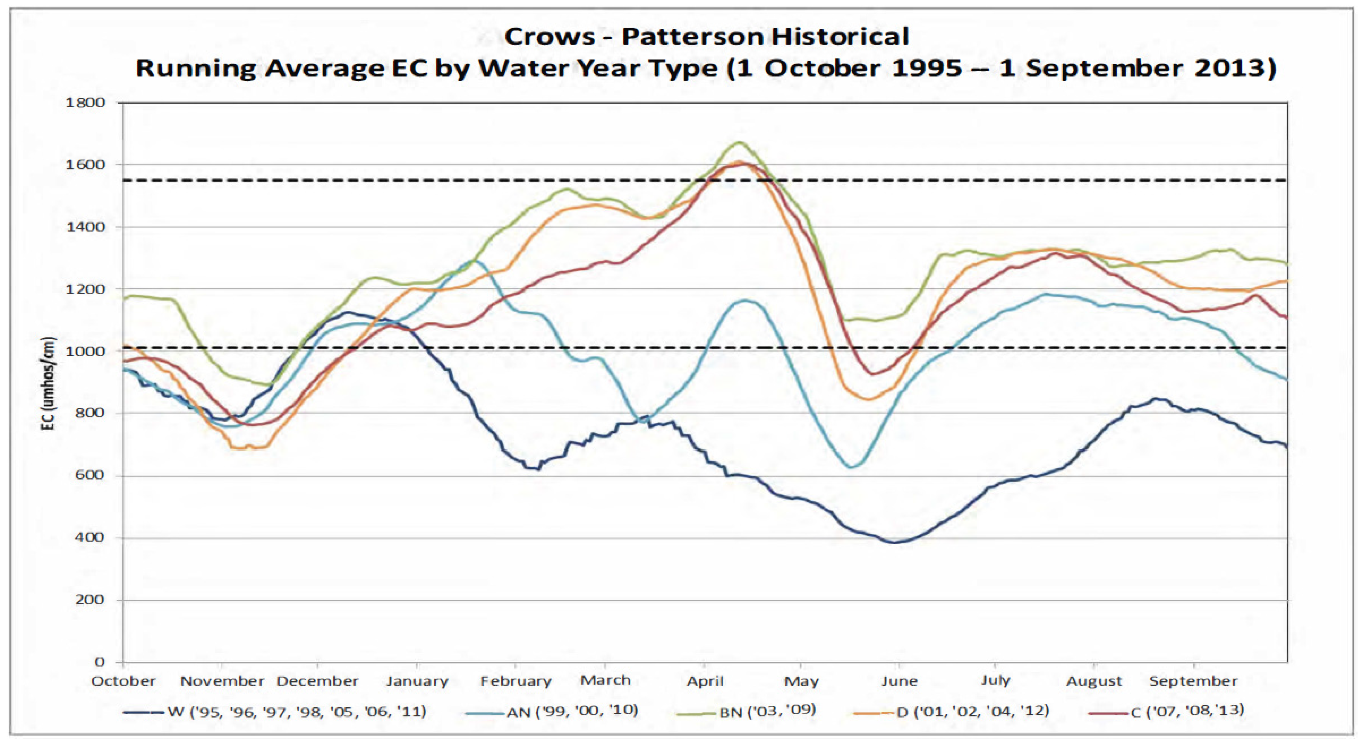
In December 2018 the Environmental Protection Agency approved a Regional Water Board Basin Plan amendment that established upstream objectives at the Maze and Crows Landing monitoring locations on the San Joaquin River. These objectives were ostensibly to protect the water quality of riparian diversions to westside San Joaquin River irrigation districts. The objectives of 1550 uS/cm apply year-round at both monitoring stations and considered the field crops and orchards farmed adjacent to this reach of the river. Figure 3 and Figure 4 show the 30-day running average EC at the Maze and Crows Landing compliance monitoring stations for the period 1 October 1995 through 1 September 2013. At Maze Road some of the highest EC values occurred in below-normal years as opposed to dry and critically dry years, although, all the data appear well below the 1550 uS/cm concentration objective. Maze Road is downstream of the Tuolumne River which appears to provide adequate dilution flow year-round. On the other hand, the Crows Landing site did show exceedances of the 1550 uS/cm objective during April for all three water year types (below normal, dry, and critically dry). Since the Vernalis compliance monitoring station is downstream of the Stanislaus River and was obligated to meet the winter 1000 uS/cm objective and 700 uS/cm objective through controlled releases by the USBR through their New Melones Reservoir operation, the incidence of exceedance was largely eliminated at this site [33,34].
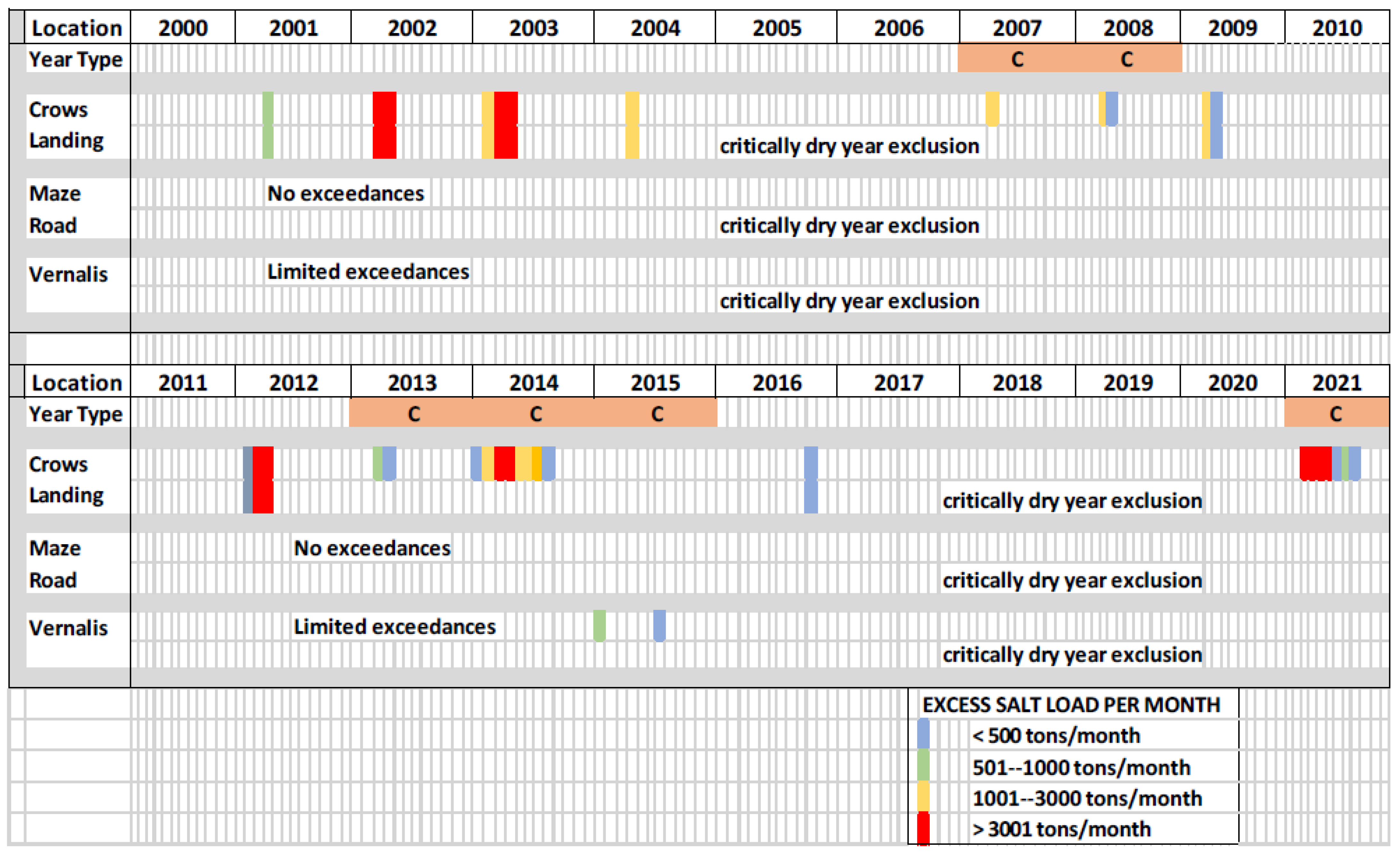
An analysis of the 30-day running average EC was subsequently conducted for all three compliance monitoring stations using more decent data for a 21-year period between 2000 and 2021. The same logic was applied as in the prior Regional Water Board compliance penalty analysis [35], although in this instance a second policy was introduced that imposed a fine of USD 10 per ton of salt. This fine schedule was chosen ostensibly to be a round number that produced an outcome of similar magnitude to the first policy when the 30-day running average monthly objective was exceeded. Figure 5 is a bar chart showing the frequency (number of days) that the 30-day running average EC was exceeded at each of the compliance monitoring stations. In Table 2 and Table 3 the potential fines were compared for the two policies for each month of the 21-year period. Note that this is a slight variation of the prior Regional Water Board policy, which imposed a penalty for all days of the month anytime the 30-day running average EC was exceeded in any month. With the use of the WARMF forecasting model and decision support system, calculation of the 30-day running average has become routine and provided a more equitable policy outcome. With better online real-time access to estimated salt load from each of the seven subareas the response time for remedial actions on the river was reduced. However, an institutional mechanism for deciding real-time actions has still to be ratified by designated resource managers for each of the seven subareas contributing salt load to the San Joaquin River.
The summary provided in Table 2 and Table 3 shows that the Crows Landing station is largely controlling salt management in the San Joaquin River. Hence, actions to achieve compliance with the Crows Landing objectives need to be implemented in the three subareas upstream of this compliance monitoring site. This would include the Grasslands, San Joaquin River Above Salt Slough and Merced River catchment subareas (Figure 2). The Grasslands subarea comprises agricultural, wetland, and municipal stakeholders and a cost-effective equitable response would need to be developed among these entities. The majority of exceedances at the Crows Landing compliance monitoring station occurred in the months of March–May (Figure 4), which coincided with the wetland drawdown period when irrigated agriculture in the subarea was also providing pre-irrigation to field crops and orchards. Although the last 20 years have seen a significant move to drip irrigation, more water conserving technologies and selenium management practices have eliminated a major source of salt load from the subarea. Subsurface tile drainage is now diverted to a dedicated 6000+ acres of reuse area, thus, any response would be expected to include actions from all three entities. Managed seasonal wetlands in the Grasslands subarea are constrained by the fact that any significant delay in wetland drainage from the 160 private duck clubs and state and federal refuge wetland complexes can change the germination success of high-value grasses potentially leading to lower value habitat for the overwintering waterfowl that rely on this resource [37,38]. Irrigated agriculture may need to invest in additional temporary storage ponds in areas free of selenium in shallow groundwater (selenium is a potential toxin when drainage concentrations exceed 5 ppb) or automation of sump pumps and new drainage conveyance plumbing to facilitate salt management through reuse and drainage recirculation. Municipal discharge of salts in the Grassland sub-basin is minimal with most ponded water being eliminated through seepage to groundwater. Municipal wastewater facilities may own storage ponds that might be usable and temporary storage facilities to reduce salt loading from the Grassland subarea. The potential for this cooperative and coordinated salt management strategy is unknown at this time. In the Merced River catchment subarea, the salt load contribution to the river is dominated by the reservoir releases from the McSwain and New Exchequer Dams and irrigation return flows into the Merced River. The Merced National Wildlife refuge contributes an insignificant return flow given its reliance on groundwater as the water supply source. The subarea south of Salt Slough is bottomland in the Valley trough and contributes to the San Joaquin River through groundwater seepage. Reservoir releases from Friant Dam can be diverted into the subarea through riparian pumping. Seepage may occur from the river into the subarea in response to local groundwater pumping.
3.3. Economic Analysis of Selected Salt Management Strategies
The first part of this paper laid out the theoretical underpinning and principles of a collaborative strategy that was anticipated would be necessary by the state regulator and that is necessary to achieve cost-effective and equitable salt management strategies. The cost and institutional feasibility of these strategies should be juxtaposed against paying the fine that the Regional Water Board has formulated to provide an incentive for regional basin cooperation and coordination without creating an undue burden on stakeholders or incentivizing stakeholder litigation. The seven subareas were chosen, not only from a hydrological perspective but also from a jurisdictional and institutional viewpoint. This paper now provides an economic rationale for a couple of effective salt management strategies that were proposed for consideration in the region.
We start by comparing the strategy of building and maintaining temporary holding ponds to store salt loads until they can be safely discharged to the San Joaquin River without exceeding objectives at any of the three compliance monitoring sites. Other means of providing temporary storage are surface and subsurface drainage reuse or short-term storage of salt load in the shallow groundwater, achieved by temporarily switching off tile drainage sump pumps. The analyses in [39], and prior in the United States Department of the Interior, Bureau of Reclamation model report [40], provide realistic cost parameters for various temporary salt storage options relevant to real-time management of salt loading to the San Joaquin River.
The CDM Smith report [39], refers to two regions that can be relevant to two of our sub areas: Tulare Lake Bed (TLB) (Note that the Tulare Lake bed is outside our study area. It does not export salt to the San Joaquin River. However, the costs of ponds may be relevant to our study.) and San Joaquin River Quality Improvement Project (SJRIP). Table 4 summarizes the relevant results to our work from the report of [39].
We used the observed data for the region during 2001 through 2021 as the basis for calculating the excess annual salt load above the regional allowances that could either be disposed of to the river with an excess fine paid, or be temporarily stored and reduced through reuse, recirculation, or storage in the shallow groundwater system (shut off sump pumping). The cost values in Table 4 are based on several assumptions. First, it is assumed that the cost per ton of salt stored in the pond include variable, fixed, and the opportunity cost of the land assigned to the pond. We used the working assumption in [39], without changing them.
The pond technology in [39], was assessed in two regions in the Central Valley. However, in our analysis we used the cost and effectiveness values in each region as our higher and lower values within which the technology performed. One set of values suggested that it took USD 9.62 per ton of stored salt and with an effectiveness rate of 90%. The second set of values suggested a USD 24.72 per ton of temporary storage of salt with an effective rate of 11% (Table 4).
Salt load that exceeded the allowance for disposal was subject to a fine. Taxes were either by days of exceedance of salt concentration or by total tons of salt above the level of allowance (Table 2 and Table 3). The analysis in this paper refers only to tons of salt observed on a monthly basis between 2001 and 2021. Two levels of fine rates have been arbitrarily used (USD 10/ton and USD 20/ton) to reflect incentive–provision fines on the part of the stakeholders in the subarea. Since the analysis spans over 20 years (2001–2021) we used a discount rate to allow comparisons of sums between 2001 and 2021. We used the directive for using a real discount rate of 7% [41]. That source requires the use also of a 3% discount rate, but for our purposes this was not necessary.
The WARMF model provided the salt load allocation for each of the seven subareas that was developed for the Real-Time Program by the Regional Water Quality Control Board based on the original salt load TMDL. These salt load allocations provide an initial basis for negotiation and allow the excess salt loads over and above the subarea allocation to be calculated. If treated, we applied the cost and effectiveness parameters to calculate the treatment cost. Since effectiveness is always less than 100%, the remainder of the salt to be disposed of was subject to the fine. Then, we compared the total annual cost of treating the salt plus paying the incremental fee to the total annual cost in the case that the salt load is not treated and is disposed of in its entirety.
4. Results and Discussion
4.1. Results
Table 5 presents the results of our analysis under the various assumptions regarding the parameters we presented earlier.
The results provide a clear distinction between the different scenarios: efficient-inexpensive-low fine ((90%; USD 9.62/ton); USD 10/ton); inefficient-expensive-low fine ((1%; USD 24.72/ton); USD 10/ton); efficient-inexpensive-high fine ((90%; USD 9.62/ton); USD 20/ton); and inefficient-expensive-high fine ((1%; USD 24.72/ton); USD 20/ton), which are reflected in Table 5. Clearly seen are the suggestions that, in three out of the four scenarios, the net present value of the differences between the fee payments for the total managed salt load and the storage or reuse cost plus the fee payment for the remainder of the unmanaged salt suggest that the subarea should not engage in managing the salt and should pay the cost of the fine. Only under the scenario of a high level of fee per ton and efficient and inexpensive treatment, the difference between the costs was positive, suggesting that treatment is justified.
4.2. Discussion
As California battles another year of drought; records are being broken for climate extreme conditions impacting the sustainability of water resources and human-induced problems of water scarcity, quality, and misallocation. The State of California has taken aggressive action starting in 2014 with the passage of the Sustainable Groundwater Management Act and the formation of the stakeholder-led Central Valley salinity Coalition (CVSALTS) that together address problems of unsustainable groundwater pumping practices, problems of subsidence and water quality degradation of surface and groundwater resources, and the fertility of agricultural soils. Although salinity degradation of receiving waters, such as rivers and deep percolation of saline water to aquifers, have been studied for over 100 years and are well understood, there has been a reluctance of the state to commit to addressing this problem. The publication of the 2002 Total Maximum Daily Load (TMDL) by the federal EPA for salt and boron incentivized the search for effective and cost-effective policy tools to address salinity impairments in the San Joaquin River and to find a feasible and equitable schema that would be accepted by stakeholders and foreclose costly litigation that would result in a continuation of the status quo.
TMDL required the state government water quality regulator to set salt load objectives for the basin in 2002. However, the conservative nature of the TMDL computation and utilizing the lowest 10% average low-flow condition resulted in allocations that were unattainable without a major impact to the agricultural economy in each subarea. This created a need to replace the initial TMDL allocations with more flexible concentration objectives based on a 30-day running average electrical conductivity (EC) that will accommodate agricultural production and irrigation practices. A concentration objective allows agricultural producers and other salinity dischargers to utilize more of the available salt load assimilative capacity in the SJR. This initial compliance monitoring objective has been supplemented with two additional upstream salinity objectives, ostensibly, to protect the water quality of agricultural diversions made by westside agricultural producers.
The adjustments of the quality standards to seasons and to the different locations (subareas) and the real-time reporting to the stakeholders allow farmers more flexibility in adjusting their practices and responding to the standards in a creative way. In that respect, the approach suggested in our work is similar to Doole [21], and Doole and Pannell [22], which take into account the differences in abatement cost and ability to address quality standards by different dairy farms in New Zealand. Hence, a differential standard is suggested for more cost-effective results at the regional level.
Adjustment of the salinity standard to the conditions in the river assimilative capacity and in each subarea along the river also allows introduction of trade in salinity disposal permissions among subareas as another way of handling the salinity load to the river. In that respect, the experience of the Hunter Basin of New South Wales, Australia [25,26], is similar to the suggested scheme in the SJR as discussed in our paper. The main idea of the scheme in the Hunter was to permit discharge of salt loads only when there was available salt load assimilative capacity in the river that drains the Hunter Basin. Details in Quinn [4], explain how salt load discharges to the river were scheduled by quantity, time, and location, based on stakeholder need and calculations of salt load assimilative capacity using a simple spreadsheet mass–balance model. While our work has not explored regional cooperative arrangements, such as trade in salt load permissions, or side payments for improvements in on-farm salinity load disposal, our future work will focus on such options.
5. Conclusions and Policy Implication
This paper presents an alternative approach to salt regulation and control that follows first attempts to implement the 2002 TMDL, when it was realized that TMDL policy objectives could not be achieved without potential annual costs to stakeholders in the millions of dollars annually, using typical penalty schedules for daily exceedance of a 30-day running average EC objective at a single downstream compliance site. These costs would have potentially risen with the inclusion of two additional upstream compliance monitoring sites adopted to protect agricultural riparian diverters from high salt concentrations in irrigation applied water. The novel concept of “Real-Time Water Quality management” relies on a continually updated forecasting model to provide daily estimates of salt load assimilative capacity in the San Joaquin River and assessments of compliance with salinity concentration objectives at three monitoring sites on the river, based on the 30-day running average EC. A water quality forecasting model WARMF was developed as part of this alternative regulatory schema, which served both as a compliance forecasting tool and the means by which salt load allocations and salt exports from each of the seven contributing subareas could be estimated and compared. The trading of salt loads between subareas is now feasible as both the regulatory salt load allocation and actual salt load discharge to the river can be quantified. The results of the study have shown that the policy combination of well-crafted river salinity objectives by the regulator and the application of an easy-to use and maintain decision support tool by stakeholders have succeeded in minimizing water quality (salinity) exceedances over a 20-year study period. The WARMF model improvements, and consequent increase in stakeholder and agency confidence in this decision support tool, suggest its potential application in other river basins facing similar challenges. Our framework allows farmers and regulators to jointly understand and evaluate the meaning of various regulatory policy interventions on the emission of salinity and on the cost to be incurred by farmers at various locations along the river. The results of the paper support the development of close collaboration between farmers and regulators in the application of non-point source pollution policy. The paper also suggests significant benefit from better cooperation and coordination among and between farmers and other dischargers of salt load who rely on the river for drainage disposal and who are already organized into sensible subareas for salt management. This can provide a cost-effective pathway for agricultural sustainability.
Author Contributions
Conceptualization, A.D. and N.W.T.Q.; methodology, A.D. and N.W.T.Q.; validation, A.D. and N.W.T.Q.; formal analysis, A.D. and N.W.T.Q.; investigation, A.D. and N.W.T.Q.; resources, A.D.; data curation, A.D. and N.W.T.Q.; writing—original draft preparation, A.D.; writing—review and editing, A.D. and N.W.T.Q.; supervision, A.D. All authors have read and agreed to the published version of the manuscript.
Funding
This research was funded, in part, by the Gianni Foundation Mini-grant Program 2020 DAVIS CA, 95616, USA.
Institutional Review Board Statement
Not applicable.
Informed Consent Statement
Not applicable.
Data Availability Statement
All data used in this paper is reported in the various tables. Additional clarifications regarding the data can be obtained from the corresponding author upon request.
Acknowledgments
The work leading to this paper was funded by the Giannini Foundation of Agricultural Economics Mini-grant Program. Ariel Dinar would like to acknowledge support from the W4190 Multistate NIFA-USDA-funded project, “Management and Policy Challenges in a Water-Scarce World”. Financial support for the development of the real-time salinity management concept has been provided by the US Bureau of Reclamation, Division of Planning, and the California Department of Water Resources through Proposition 84- funded grants.
Conflicts of Interest
The authors declare no conflict of interest.
References
- Tanji, K.K.; Kielen, K.C. Agricultural Drainage Water Management in Arid and Semi-Arid Areas; FAO Irrigation and Drainage Paper 61; Food and Agriculture Organization of the United Nations: Rome, Italy, 2002. [Google Scholar]
- Hart, B.; Walker, G.; Katupitiya, A.; Doolan, J. Salinity Management in the Murray–Darling Basin, Australia. Water 2020, 12, 1829. [Google Scholar] [CrossRef]
- Baccour, S.; Albiac, J.; Kahil, T.; Esteban, E.; Crespo, D.; Dinar, A. Hydroeconomic modeling for assessing water scarcity and agricultural pollution abatement policies in the Ebro River Basin, Spain. J. Clean. Prod. 2021, 327, 129459. [Google Scholar] [CrossRef]
- Quinn, N.W.T. Adaptive implementation of information technology for real-time, basin-scale salinity management in the San Joaquin Basin, USA and Hunter River Basin, Australia. Agric. Water Manag. 2011, 98, 930–940. [Google Scholar] [CrossRef]
- Obropta, C.C.; Niazi, M.; Kardos, J.S. Application of an environmental decision support system to a water quality trading program affected by surface water diversions. Environ. Manag. 2008, 42, 946–956. [Google Scholar] [CrossRef] [PubMed]
- Zhang, X.; Huang, G.H.; Nie, X.; Lin, Q. Model-based decision support system for water quality management under hybrid uncertainty. Expert Syst. Appl. 2011, 38, 2809–2816. [Google Scholar] [CrossRef]
- Ioannou, K.; Lefakis, P.; Arabatzis, G. Development of a decision support system for the study of an area after the occurrence of forest fire. Int. J. Sustain. Soc. 2011, 3, 5–32. [Google Scholar] [CrossRef]
- Makropoulos, C.K.; Natsis, K.; Liu, S.; Mittas, K.; Butler, D. Decision support for sustainable option selection in integrated urban water management. Environ. Model. Softw. 2008, 23, 1448–1460. [Google Scholar] [CrossRef]
- Rose, D.C.; Sutherland, W.J.; Parker, C.; Lobley, M.; Winter, M.; Morris, C.; Twining, S.; Ffoulkes, C.; Amano, T.; Dicks, L.V. Decision support tools for agriculture: Towards effective design and delivery. Agric. Syst. 2016, 149, 165–174. [Google Scholar] [CrossRef] [Green Version]
- Systech Water Resources, Inc. Watershed Analysis Risk Management Framework (WARMF): Technical Model Documentation; Systech Water Resources, Inc.: Walnut Creek, CA, USA, 2017. [Google Scholar]
- Quinn, N.W.T.; Tansey, M.K.; Lu, J. Comparison of Deterministic and Statistical Models for Water Quality Compliance Forecasting in the San Joaquin River Basin, California. Water 2021, 13, 2661. [Google Scholar] [CrossRef]
- Fu, B.; Horsburgh, J.S.; Jakeman, A.J.; Gualtieri, C.; Arnold, T.; Marshall, L.; Green, T.R.; Quinn, N.W.T.; Volk, M.; Hunt, R.J.; et al. Modeling water quality in watersheds: From here to the next generation. Water Resour. Res. 2020, 56, e2020WR027721. [Google Scholar] [CrossRef]
- Quinn, N.W.T.; Hughes, B.; Osti, A.; Herr, J.; Wang, J. Real-time, web-based decision support for stakeholder implementation of basin-scale salinity management. In Environmental Software Systems: Computer Science for Environmental Protection, Proceedings of the 12th IFIP WG 5.11 International Symposium, ISESS 2017, Zadar, Croatia, 10–12 May 2017; Hrebicek, J., Denzer, R., Schimak, G., Pitner, T., Eds.; Springer: Cham, Switzerland, 2018. [Google Scholar]
- Griffin, R.C.; Bromley, D.W. Agricultural runoff as a nonpoint externality: A theoretical development. Am. J. Agric. Econ. 1982, 64, 547–552. [Google Scholar] [CrossRef]
- Shortle, J.S.; Dunn, J.W. The relative efficiency of agricultural source water pollution. Am. J. Agric. Econ. 1986, 68, 668–677. [Google Scholar] [CrossRef]
- Shortle, J.S.; Abler, D.G.; Horan, R.D. Research issues in nonpoint pollution control. Environ. Resour. Econ. 1998, 11, 571–585. [Google Scholar] [CrossRef]
- Larson, D.M.; Helfand, G.E.; House, B.W. Second best tax policies to reduce nonpoint source pollution. Am. J. Agric. Econ. 1996, 78, 1108–1117. [Google Scholar] [CrossRef] [Green Version]
- Ribaudo, M.; Horan, R.D.; Smith, M.E. Economics of Water Quality Protection from Nonpoint Sources: Theory and Practice; Agricultural Economic Report No. 782; Resource Economics Division, Economic Research Service, U.S. Department of Agriculture: Washington, DC, USA, 1999. [Google Scholar]
- Kolstad, C.D. Uniformity versus differentiation in regulating externalities. J. Environ. Econ. Manag. 1987, 14, 386–399. [Google Scholar] [CrossRef]
- Wu, J.; Babcock, B.A. Babcock. Spatial heterogeneity and the choice of instruments to control nonpoint pollution. Environ. Resour. Econ. 2001, 18, 173–192. [Google Scholar] [CrossRef]
- Doole, G.J. Evaluating input standards for nonpoint pollution control under firm heterogeneity. J. Agric. Econ. 2010, 61, 680–696. [Google Scholar] [CrossRef]
- Doole, G.J.; Pannell, D.J. Empirical evaluation on nonpoint pollution policies under agent heterogeneity: Regulating intensive dairy production in the Waikato Region of New Zealand. Aust. J. Agric. Resour. Econ. 2011, 56, 82–101. [Google Scholar] [CrossRef] [Green Version]
- Esteban, E.; Albiac, J. Salinity pollution control in the presence of farm heterogeneity: An empirical analysis. Water Econ. Policy 2016, 2, 1650017. [Google Scholar] [CrossRef]
- Murray-Darling Basin Authority. Basin Salinity Management Strategy 2001–2015. Australian Government. 2001. Available online: https://www.mdba.gov.au/sites/default/files/pubs/BSMS-full.pdf (accessed on 31 July 2022).
- Department of Environment and Conservation, New South Wales, Australia. Hunter River Salinity Trading Scheme: Working Together to Protect River Quality and Sustain Economic Development. 2003. Available online: https://www.cbd.int/financial/pes/australia-pesriver.pdf (accessed on 31 July 2022).
- NSW Minerals Council. Review of Hunter River Salinity Trading Scheme. 2014. Available online: https://www.epa.nsw.gov.au/-/media/epa/corporate-site/resources/licensing/hrsts/nsw-minerals-council.pdf (accessed on 31 July 2022).
- Yaron, D.; Ratner, A. Regional cooperation in the use of irrigation water: Efficiency and income distribution. Agric. Econ. 1990, 4, 45–58. [Google Scholar] [CrossRef]
- Dinar, A.; Ratner, A.; Yaron, D. Evaluating cooperative game theory in water resources. Theory Decis. 1992, 32, 1–20. [Google Scholar] [CrossRef]
- Nicholson, F.; Laursen, R.K.; Cassidy, R.; Farrow, L.; Tendler, L.; Williams, J.; Surdyk, N.; Velthof, G. How Can Decision Support Tools Help Reduce Nitrate and Pesticide Pollution from Agriculture? A Literature Review and Practical Insights from the EU FAIRWAY Project. Water 2020, 12, 768. [Google Scholar] [CrossRef]
- Chowdary, V.; Rao, N.; Sarma, P. Decision support framework for assessment of non-point-source pollution of groundwater in large irrigation projects. Agric. Water Manag. 2005, 75, 194–225. [Google Scholar] [CrossRef]
- Mas-Colell, A.; Whinston, M.D.; Green, J.R. Chapter 16: Equilibrium and Its Basic Welfare Properties. In Microeconomic Theory; Oxford University Press: Oxford, UK, 1995. [Google Scholar]
- Dinar, A.; Howitt, R.E. Mechanisms for allocation of environmental cost: Empirical tests of acceptability and stability. J. Environ. Manag. 1997, 49, 183–203. [Google Scholar] [CrossRef]
- (RWQCB) California Environmental Protection Agency, (CalEPA) Regional Water Quality Control Board, Central Valley Region. Total Maximum Daily Load for Salinity and Boron in the Lower San Joaquin River; Staff Report; Califorinia Environmental Protection Agency, Regional Water Quality Control Board, Central Valley Region: Sacramento, CA, USA, 2002. [Google Scholar]
- (RWQCB) California Environmental Protection Agency, (CalEPA) Regional Water Quality Control Board, Central Valley Region. Amendments to the Water Quality Control Plan for the Sacramento River and San Joaquin River Basins for the Control of Salt and Boron Discharges into the Lower San Joaquin River; Final Staff Report; California Environmental Protection Agency, Regional Water Quality Control Board, Central Valley Region: Sacramento, CA, USA, 2004.
- Brownell, J.; (Regional Water Quality Control Board, Central Valley Region, Rancho Cordova, CA 95670, USA). Personal communication, 2013.
- (LWA) Larry Walker Associates, Inc.; Systech Water Resources; Carollo Engineers; PlanTierra. Development of a Basin Plan Amendment for Salt and Boron in the Lower San Joaquin River (LSJR)—Task 4 Implementation Planning for Proposed Salinity Objectives; San Joaquin Valley Drainage Authority: Los Banos, CA, USA, 2015. [Google Scholar]
- Quinn, N.W.T.; Hanna, W.M. Real-Time Adaptive Management of Seasonal Wetlands to Improve Water Quality in the San Joaquin River. Adv. Environ. Res. 2002, 5, 309–317. [Google Scholar] [CrossRef]
- Ortega, R. Swamp Timothy Production Response to a Modified Hydrology in Wetlands of the Grassland Ecological Area. Master’s Thesis, Department of Avian Studies, UC Davis, Davis, CA, California, 2009. [Google Scholar]
- CDM Smith. Central Valley Salinity Alternatives for Long-Term Sustainability (CV-Salts). Strategic Salt Accumulation Land and Transportation Study (SSALTS), Draft Phase 3 Report–Evaluate Potential Salt Disposal Alternatives to Identify Acceptable Alternatives for Implementation; Prepared for San Joaquin Valley Drainage Authority, October 2016; CDM Smith: Boston, MA, USA, 2016. [Google Scholar]
- United States Department of the Interior, Bureau of Reclamation, San Luis Unit Drainage, Central Valley Project, California, Fresno, Merced, and Kings Counties. Draft Environmental Impact Statement; Report S621.M531 1991; United States. Bureau of Reclamation. Mid-Pacific Regional Office: Sacramento, CA, USA, 1991.
- (OMB) US Office of Management and Budget. 2021 Discount Rates. 2021. Available online: https://www.energy.gov/sites/default/files/2021-04/2021discountrates.pdf (accessed on 17 April 2022).
Figure 1.
A schematic representation of the region with subareas, agricultural producers, and a regulated receiving water body (river).
Figure 1.
A schematic representation of the region with subareas, agricultural producers, and a regulated receiving water body (river).

Figure 2.
Map of the various San Joaquin River Basin contributing subareas as defined in the 2002 TMDL Regulation Plan: Northwest Side (NWS), Grasslands Agriculture (GRA), East Valley Floor (EVF), Merced River (MER), Stanislaus River (STL), Tuolumne River (TLU), and San Joaquin River above Salt Slough (SJR). Note: the eight red triangles in the Figure that are indicated in the legend by numbers 1–8 are the locations of the flow and salinity load monitoring stations. Source: [33,34].

Figure 3.
Maze Road Historical 30-day Running Average EC by Water Year Type [36].
Figure 3.
Maze Road Historical 30-day Running Average EC by Water Year Type [36].

Figure 4.
Crows Landing Historical 30-day Running Average EC by Water Year Type [36].
Figure 4.
Crows Landing Historical 30-day Running Average EC by Water Year Type [36].

Figure 5.
Exceedance frequency of 30-day running average EC at all three compliance monitoring stations of the San Joaquin River for 21 years: 2000–2021.
Figure 5.
Exceedance frequency of 30-day running average EC at all three compliance monitoring stations of the San Joaquin River for 21 years: 2000–2021.


Table 1.
Potential Salt Discharge Load Exceedance Fees by subarea (2001–2012), ref. [35].
Table 1.
Potential Salt Discharge Load Exceedance Fees by subarea (2001–2012), ref. [35].
| Subarea | NWS | GL | SJR | EVF | |
|---|---|---|---|---|---|
| Days exceeded by period | Oct | 0 | 0 | 0 | 0 |
| Nov | 90 | 60 | 0 | 0 | |
| Dec | 124 | 248 | 0 | 0 | |
| Jan | 186 | 0 | 310 | 0 | |
| Feb | 28 | 196 | 0 | 0 | |
| Mar | 0 | 279 | 0 | 0 | |
| Apr | 28 | 56 | 42 | 14 | |
| VAMP a | 0 | 0 | 30 | 30 | |
| May | 0 | 0 | 51 | 17 | |
| Jun | 30 | 30 | 210 | 90 | |
| Jul | 0 | 0 | 248 | 91 | |
| Aug | 0 | 0 | 248 | 31 | |
| Sep | 0 | 0 | 0 | 0 | |
| Total days of exceedances | 486 | 869 | 1139 | 273 | |
| Total penalties [US$5000 per day penalty] | US$2,430,000 | US$4,345,000 | US$5,695,000 | US$1,365,000 | |
| Years calculated | 8 | 10 | 10 | 3 | |
| Average penalty per year | US$303,750 | US$434,500 | US$569,500 | US$455,000 | |
| Subarea acreage | 118,000 | 353,000 | 187,000 | 201,000 | |
| Average penalty per acre | US$2.57 | US$1.23 | US$3.05 | US$2.26 | |
Note: a VAMP stands for Vernalis Adaptive Management Program. These were programmatic reservoir releases for fish migration that occurred each year from 15 April to 15 May. Values in the table are elaborated by the authors, based on data in [35].
Table 2.
Historical accounting on salt load exceedance, days of exceedance, monthly fees, and fine for salt load exceedance 2001–2021 at Crows Landing [36].
Table 2.
Historical accounting on salt load exceedance, days of exceedance, monthly fees, and fine for salt load exceedance 2001–2021 at Crows Landing [36].
| Month-Year | Excess Monthly Salt Load (ton) | Days of Exceedance | Monthly Fine (US$) | Fine (US$) |
|---|---|---|---|---|
| US$5000/day | US$10/ton of Salt | |||
| Apr-2001 | 552 | 12 | 60,000 | 5518 |
| Mar-2002 | 4967 | 16 | 80,000 | 49,669 |
| Apr-2002 | 4510 | 23 | 115,000 | 45,099 |
| Feb-2003 | 2238 | 18 | 90,000 | 22,377 |
| Mar-2003 | 4403 | 31 | 155,000 | 44,034 |
| Apr-2003 | 2245 | 18 | 90,000 | 22,453 |
| Apr-2004 | 2034 | 18 | 90,000 | 20,344 |
| Apr-2007 | 134 | 12 | 60,000 | 1340 |
| Apr-2008 | 1807 | 21 | 105,000 | 18,066 |
| May-2008 | 823 | 11 | 55,000 | 8233 |
| Apr-2009 | 1559 | 25 | 125,000 | 15,593 |
| May-2009 | 82 | 4 | 20,000 | 820 |
| Feb-2012 | 66 | 4 | 20,000 | 658 |
| Mar-2012 | 3374 | 31 | 155,000 | 33,743 |
| Apr-2012 | 2898 | 29 | 145,000 | 28,979 |
| Mar-2013 | 178 | 6 | 30,000 | 1777 |
| Apr-2013 | 1264 | 20 | 100,000 | 12,641 |
| Jan-2014 | 147 | 6 | 30,000 | 1474 |
| Feb-2014 | 2544 | 28 | 140,000 | 25,435 |
| Mar-2014 | 7855 | 31 | 155,000 | 78,549 |
| Apr-2014 | 7230 | 30 | 150,000 | 72,299 |
| May-2014 | 1607 | 31 | 155,000 | 16,072 |
| Jun-2014 | 1280 | 30 | 150,000 | 12,802 |
| Jul-2014 | 1132 | 31 | 155,000 | 11,321 |
| Aug-2014 | 82 | 25 | 125,000 | 823 |
| Oct-2016 | 28 | 14 | 70,000 | 280 |
| Mar-2021 | 77,514 | 27 | 135,000 | 775,145 |
| Apr-2021 | 47,752 | 30 | 150,000 | 477,518 |
| May-2021 | 30,491 | 31 | 155,000 | 304,910 |
| Jun-2021 | 4719 | 8 | 40,000 | 47,193 |
| Jul-2021 | 53 | 7 | 35,000 | 528 |
| Aug-2021 | 547 | 31 | 155,000 | 5472 |
| Sep-2021 | 14 | 5 | 25,000 | 40 |
| Total cost | US$3,320,000 | US$2,161,305 |
Note: Total cost in nominal dollars. Values elaborated by authors, based on data in [36].
Table 3.
Historical accounting on salt load exceedance, days of exceedance, monthly fees, and fine for salt load exceedance 2001–2021 at Maze Road [36].
Table 3.
Historical accounting on salt load exceedance, days of exceedance, monthly fees, and fine for salt load exceedance 2001–2021 at Maze Road [36].
| Month-Year | Excess Monthly Salt Load (ton) | Days of Exceedance | Monthly Fine (US$) US$5000/day | Fine (US$) US$10/ton of Salt |
|---|---|---|---|---|
| Jan-2015 | 727 | 14 | 70,000 | 7276 |
| Jul-2015 | 5 | 3 | 15,000 | 48 |
| Total cost | US$85,000 | US$7315 |
Notes: (1) Exceedence during the analyzed period occurred only in January and July 2015. (2) Total cost in nominal US dollars. Values elaborated by authors, based on data in [36].
Table 4.
Costs and effectiveness in removing salt of the evaporation pond technology in two locations in the Central Valley.
Table 4.
Costs and effectiveness in removing salt of the evaporation pond technology in two locations in the Central Valley.
| Region | Water Volume (AFY) | Salt Stored (Ton/Year) | Salt Accumulation (Ton) | Salt /Managed (%) | Cost/AF (US$) | Cost/Salt Stored (US$/Ton) |
|---|---|---|---|---|---|---|
| TLB | 17,240 | 139,897 | 155,479 | 90 | 76.58 | 9.62 |
| SJRIP | 19,248 | 98,108 | 890,639 | 11 | 129.62 | 24.72 |
Source: Extracted from [39], Table 2 and Table 3. Note: pond cost assumed to be equivalent to the cost of an evaporation pond. Selenium issues have pretty much nixed mixed evaporation ponds for the past 20 years. However, any selenium in drainage will warrant bird hazing and the cost of temporary holding ponds may not be that different from evaporation ponds. Values elaborated by authors, based on data in [39].
Table 5.
Cost of temporarily storing salt in surface ponds, reusing, or recirculating the salt or temporarily storing it in the shallow groundwater system under different assumptions of fee level, storage efficiency, and cost.
Table 5.
Cost of temporarily storing salt in surface ponds, reusing, or recirculating the salt or temporarily storing it in the shallow groundwater system under different assumptions of fee level, storage efficiency, and cost.
| Year with Exceedance | Salt LOAD Excess (ton) | ANNUAL Fine Payment on Stored or Reused Quantity | Annual Storage or Reused Fee Cost on Remainder of Salt Retained and Managed (US$10/ton) | Annual Fee Cost on Remainder of Salt Not Temporarily Retained and Managed (US$20/ton) | |||
|---|---|---|---|---|---|---|---|
| US$10/ton | US$20/ton | (US$9.62/ton; 90%) | (US$24.72/ton; 1%) | (US$9.62/ton; 90%) | (US$24.72/ton; 1%) | ||
| 2001 | 552 | 5520 | 11,040 | 5862 | 18,558 | 1159 | 23,471 |
| 2002 | 9477 | 94,770 | 189,540 | 100,645 | 318,616 | 19,901 | 402,962 |
| 2003 | 8886 | 88,860 | 177,720 | 94,369 | 298,747 | 18,660 | 377,832 |
| 2004 | 2034 | 20,340 | 40,680 | 21,601 | 68,383 | 4271 | 86,485 |
| 2007 | 134 | 1340 | 2680 | 1423 | 4505 | 281 | 5697 |
| 2008 | 2630 | 26,300 | 52,600 | 27,930 | 88,420 | 5523 | 111,827 |
| 2009 | 1641 | 16,410 | 16,410 | 17,427 | 55,170 | 3446 | 69,775 |
| 2012 | 6338 | 63,380 | 126,760 | 67,309 | 213,083 | 13,309 | 269,491 |
| 2013 | 1442 | 14,420 | 28,840 | 15,314 | 48,480 | 3028 | 61,313 |
| 2014 | 21,877 | 217,300 | 437,540 | 230,772 | 730,562 | 45,941 | 930,210 |
| 2015 | 732 | 7320 | 14,640 | 7773 | 24,609 | 1537 | 31,124 |
| 2016 | 28 | 280 | 560 | 297 | 941 | 59 | 1190 |
| 2021 | 161,090 | 1,610,900 | 3,221,800 | 1,710,775 | 5,415,845 | 338,289 | 6,849,547 |
| Net Present Value of Difference Between Payment for Management of Entire Salt Load and Cost of treatment and payment for incremental storage or reuse (In 2021 dollars, 7% discount rate) | −172,574 | −6,610,459 | +5,030,130 | −6,229,518 | |||
Publisher’s Note: MDPI stays neutral with regard to jurisdictional claims in published maps and institutional affiliations. |
© 2022 by the authors. Licensee MDPI, Basel, Switzerland. This article is an open access article distributed under the terms and conditions of the Creative Commons Attribution (CC BY) license (https://creativecommons.org/licenses/by/4.0/).
Share and Cite
MDPI and ACS Style
Dinar, A.; Quinn, N.W.T. Developing a Decision Support System for Regional Agricultural Nonpoint Salinity Pollution Management: Application to the San Joaquin River, California. Water 2022, 14, 2384. https://doi.org/10.3390/w14152384
AMA Style
Dinar A, Quinn NWT. Developing a Decision Support System for Regional Agricultural Nonpoint Salinity Pollution Management: Application to the San Joaquin River, California. Water. 2022; 14(15):2384. https://doi.org/10.3390/w14152384
Chicago/Turabian StyleDinar, Ariel, and Nigel W. T. Quinn. 2022. "Developing a Decision Support System for Regional Agricultural Nonpoint Salinity Pollution Management: Application to the San Joaquin River, California" Water 14, no. 15: 2384. https://doi.org/10.3390/w14152384
Note that from the first issue of 2016, this journal uses article numbers instead of page numbers. See further details here.