
Investigation of Annual Lake Water Levels and Water Volumes with Şen Innovation and Mann-Kendall Rank Correlation Trend Tests: Example of Lake Eğirdir, Turkey


 , , , , ,
Abstract
:1. Introduction
2. Materials and Methods
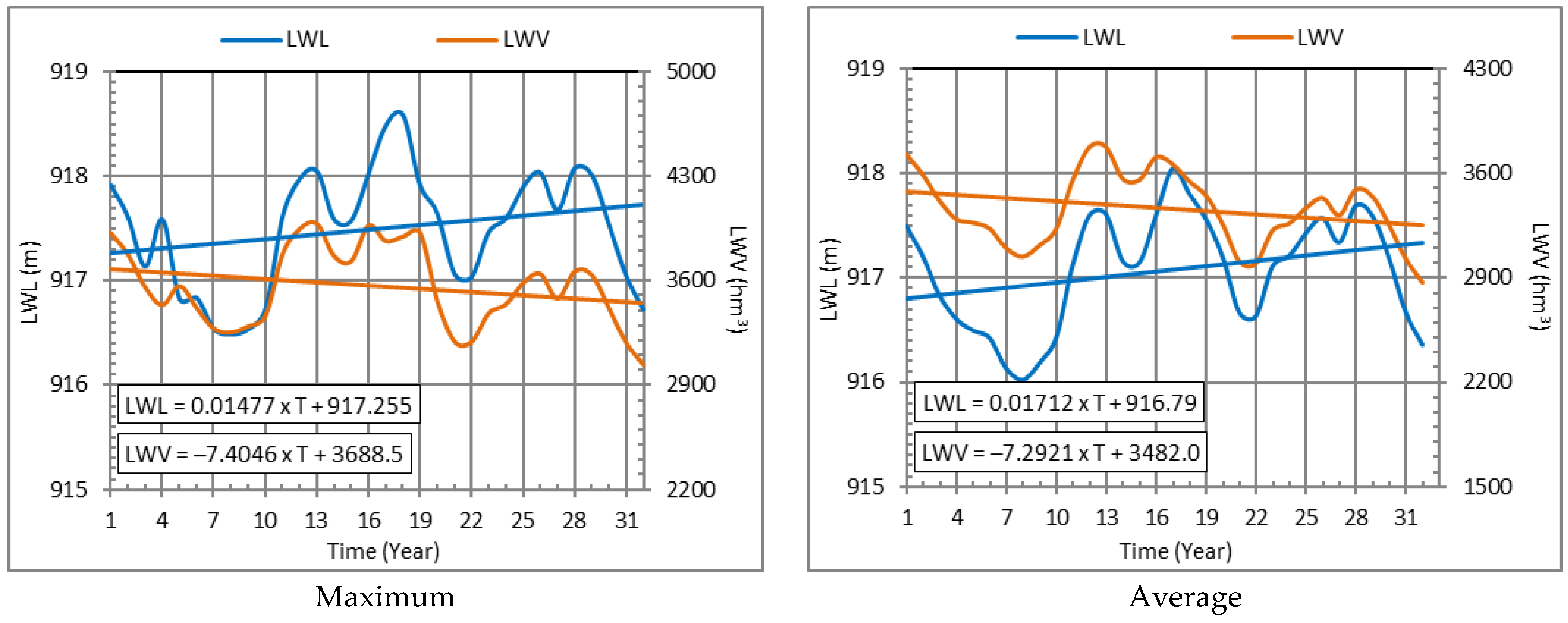
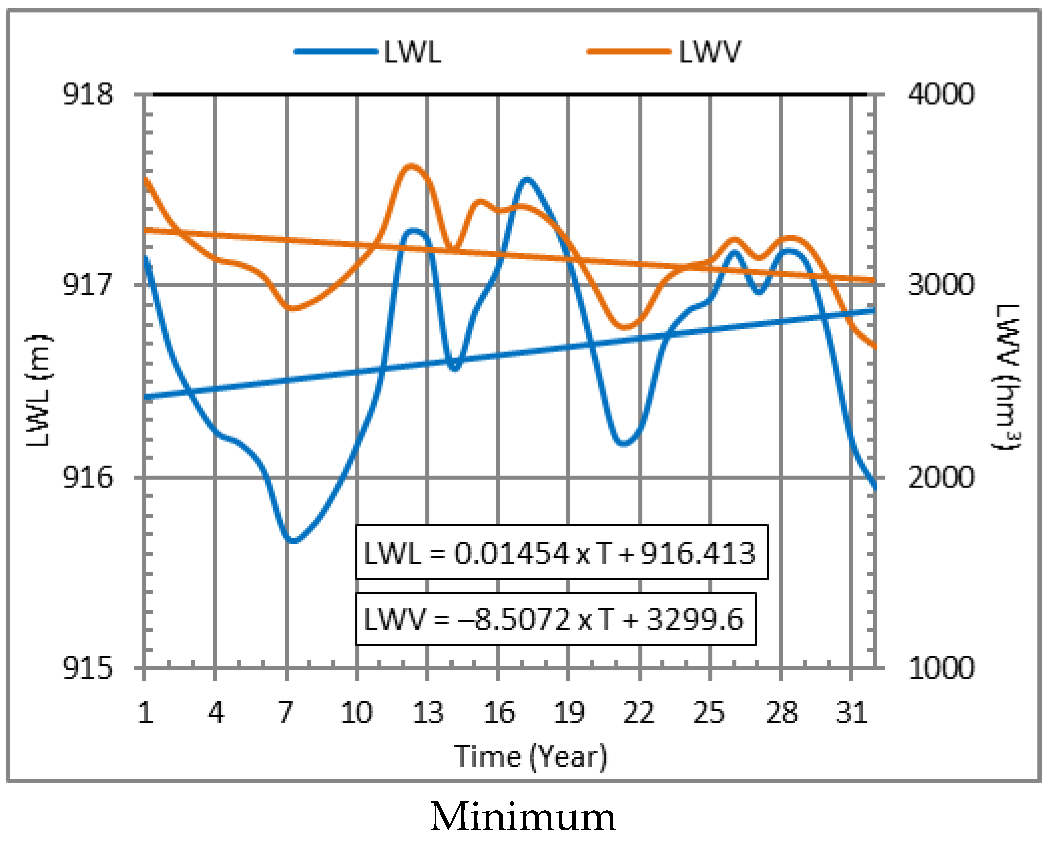
2.1. Materials
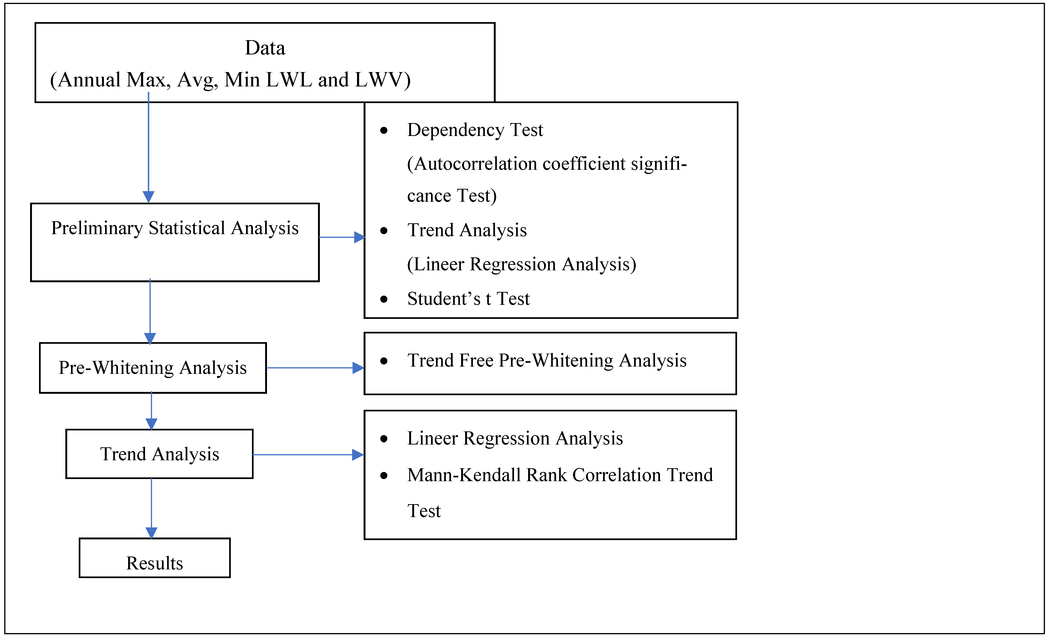
2.2. Methods
2.2.1. Dependency Test (DT)
2.2.2. Autocorrelation Coefficient Significance Test
2.2.3. Linear Regression Analysis (LRA)
- Hypothesis tests are used to test whether the coefficients are significant in the developed regression equation. The hypotheses established are: H0 = no relationship between the dependent and independent variables ( = 0), and H1 = there is a relationship between the dependent and independent variables ( ≠ 0), and it is checked whether the parameters are equal to zero.
2.2.4. t-Test (Student’s t)
- = calculated test statistic;
- , = series start and end average;
- n = number of observations;
- = standard deviation.
- = calculated test statistic;
- , = average of each sub-series;
- = standard deviation of each sub-series;
- n = total number of data in the series;
- , = number of data for each sub-series.
- = calculated test statistic;
- , = average of each sub-series;
- = variance of each subseries;
- n = total number of data in the series;
- , = number of data for each sub-series.
2.2.5. Rate of Change (CR)
- CR = rate of change (%);
- = first series average;
- = second series average.
2.2.6. Pre-Whitening Analysis (PA)
2.2.7. Trend Free Pre-Whitening
- = de-trend series;
- = chronologically ordered (t) observation series value;
- = calculated slope value of the LRA;
- = value of the de-trended series at time t;
- = de-trend series;
- = lagged-1 autocorrelation coefficient of the old (with dependency) series;
- = de-trended series at time t − 1, the recalculated lag–1 autocorrelation coefficient for the de-trended series is ().
- = re-trendless pre-adjusted series;
- = value of the de-trended series at time t;
- = calculated slope value of the LRA;
- t = chronologically ordered time.
2.2.8. Trend Test
2.2.9. Mann-Kendall Rank Correlation Trend Test (MKRCTT)
- = smaller or bigger value after its ordinal number within the ordinal numbers of the serial values;
- = total number;
- n = number of the observations;
- i = serial chronological ordinal number;
- N = total number of data in the series;
- = series average;
- var(ti) = series variance;
- = ordinal number of each data in the series;
2.2.10. Şen Innovation Trend Test (SITT)
- The slope of the trend test is calculated using Equation (13):where:
- = standard deviation;
- = the arithmetic means of each sub-series (first sub-series () and second sub-series ()) formed by dividing the dependent variable series into two;
- n = serial total number of data.
- The relative error of the trend slope is calculated using Equation (14):where:
- = relative error of the trend slope;
- = trend equation coefficient created by LRA of the new de-trended series;
- = coefficient of the LRA equation created by graphing the two lower series.
- 3.
- The cross-correlation coefficient () is calculated using Equation (15):where:
- = the arithmetic means of each sub-series (first sub-series () and second sub-series ()) formed by dividing the dependent variable series into two;
- E(E( = each subseries slope (first-order moment);
- , = variance of each subseries slope;
- = the cross-correlation coefficient between two parts.
- 4.
- The standard deviation of the trend slope is calculated using Equation (16):where:
- = standard deviation of the trend slope;
- = series variance;
- n = serial total number of data;
- = the arithmetic means of each sub-series (first sub-series () and second sub-series ()) formed by dividing the dependent variable series into two.
- 5.
- The confidence limits of the trend slope ( = upper confidence limit, = lower confidence limit) are calculated using Equation (17):
- = confidence limit;
- = standard deviation of the trend slope;
- = t distribution is the table value [65].
3. Results and Discussion
3.1. Dependency Test Results
3.2. t-Test Results
3.3. Rate of Change Results
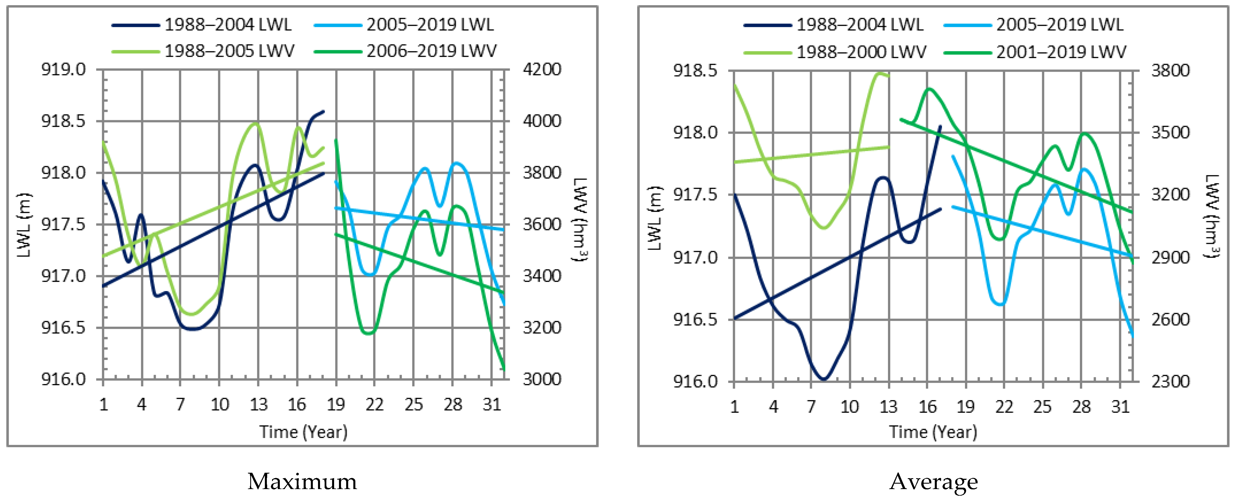
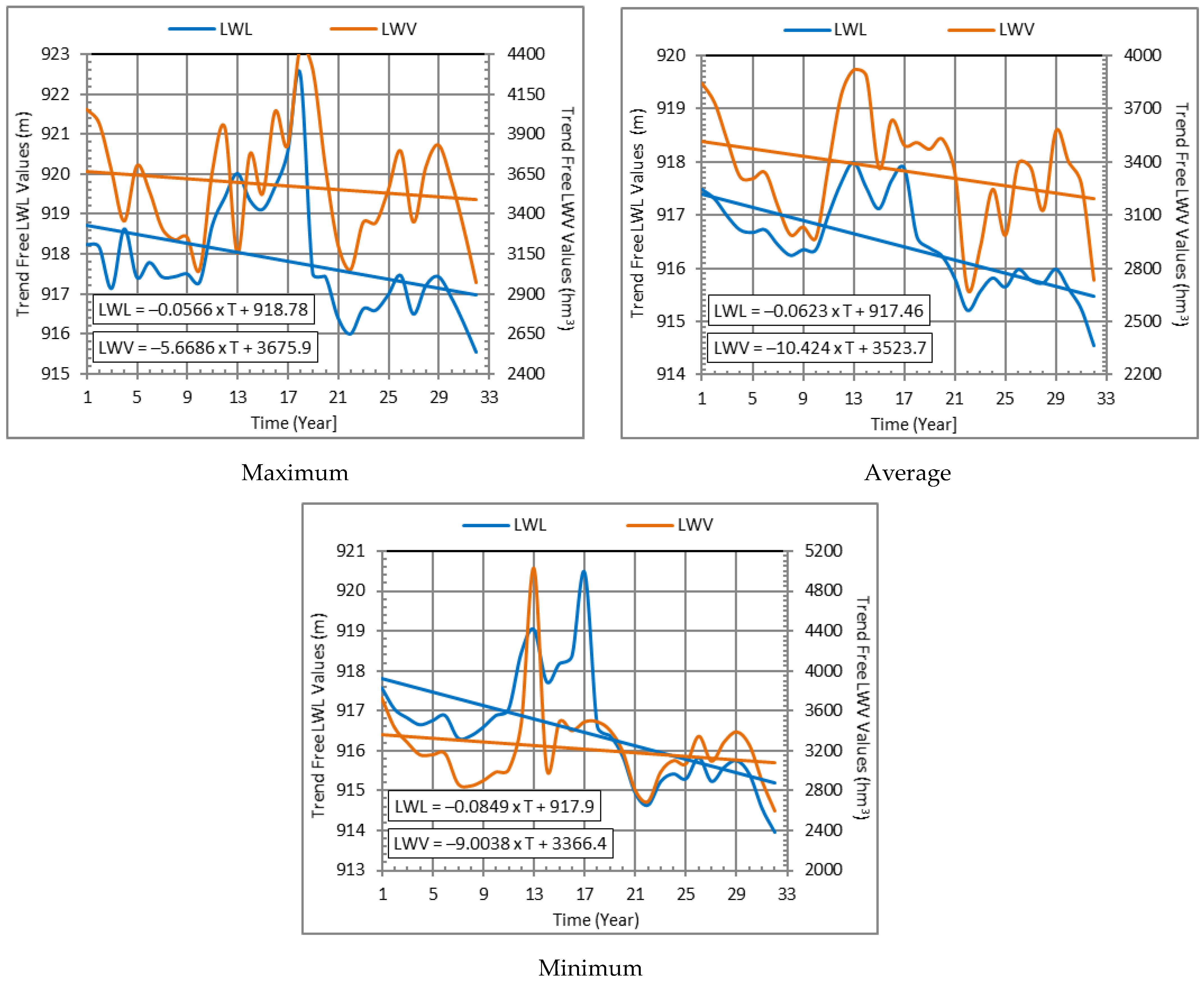
3.4. Pre-Whitening Method Results
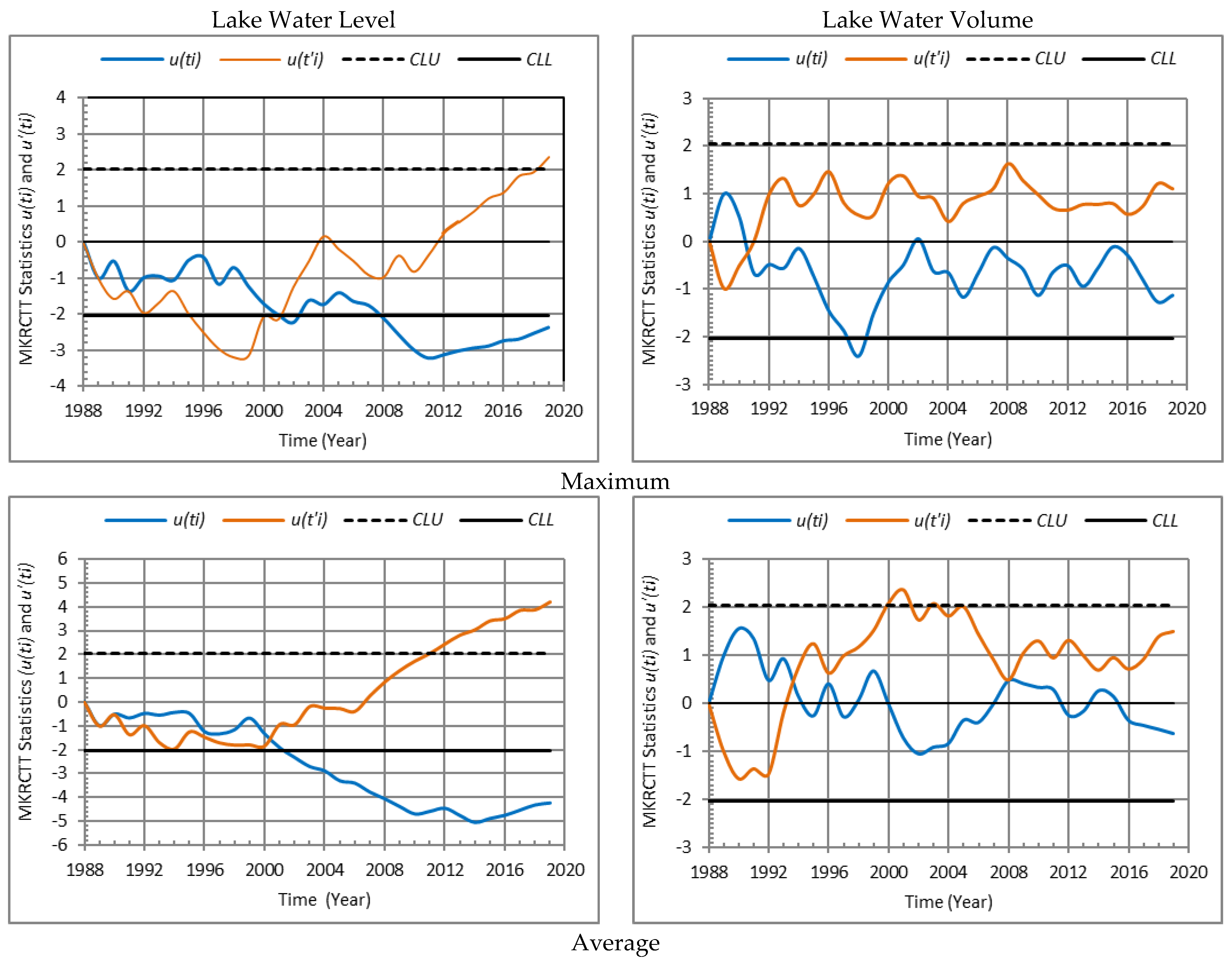
3.5. Mann-Kendall Rank Correlation Trend Test Results
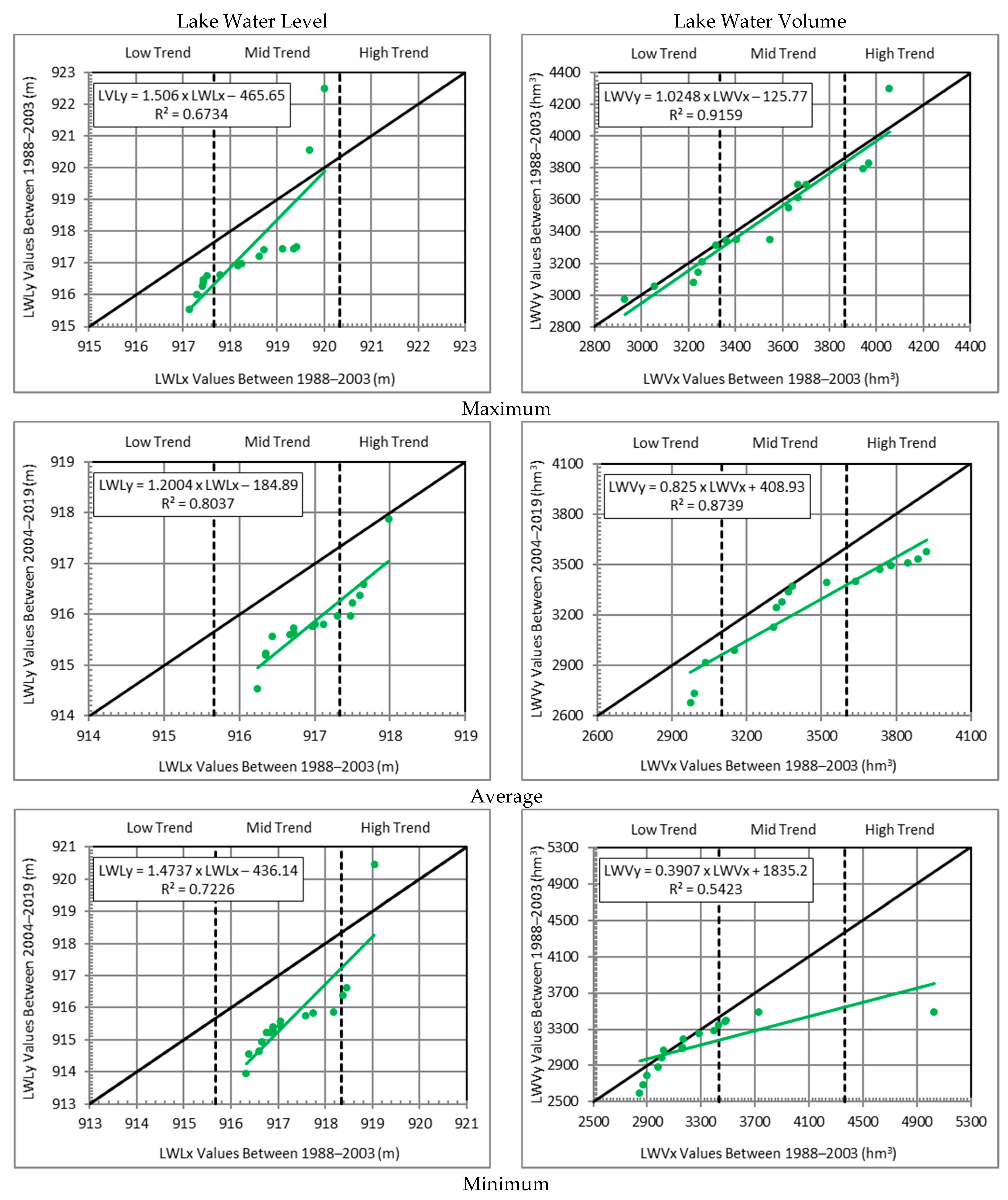
3.6. Şen Innovation Trend Test Results
4. Conclusions
Author Contributions
Funding
Institutional Review Board Statement
Informed Consent Statement
Data Availability Statement
Conflicts of Interest
References
- Akin, M.; Akin, G. Importance of Water, Water Potential in Turkey, Water Basins and Water Pollution. Ank. Univ. J. Fac. Lang. Hist. Geogr. 2007, 47, 105–118. [Google Scholar]
- Yilmaz, M.L.; Peker, H.S. A Possible Jeopardy of Water Resources in Terms of Turkey’s Economic and Political Context: Water Conflicts. J. Fac. Econ. Adm. Sci. 2013, 3, 57–74. [Google Scholar]
- Water Resources Management and Security, Specialization Commission report 11. Kalkýnma Planý. Available online: https://www.sbb.gov.tr (accessed on 10 June 2021).
- Chin, D.A. Water-Resources Engineering; Prentice Hall: Hoboken, NJ, USA, 2000. [Google Scholar]
- Gümüş, V.; Başak, A.; Oruç, N. Drought Analysis of Şanlıurfa Station with Standard Precipitation Index (SPI). Harran Univ. J. Eng. 2016, 1, 36–44. [Google Scholar]
- Büken, M.E. Assessment of Climate Change Impacts on Adana. Master’s Thesis, Çukurova Üniversitesi Fen Bilimleri Enstitüsü, Adana, Turkey, 2016. [Google Scholar]
- Biberoglu, E. Statistical Scale Reduction of Precipitation and Temperature Predictions of Global Climate Models. Ph.D. Thesis, Dokuz Eylül Üniversitesi Fen Bilimleri Enstitüsü, Izmir, Turkey, 2017. [Google Scholar]
- Dabanli, I. Climate Change Impact on Precipitation-temperature In Turkey and Drought Analysis: Akarcay Case Study. Ph.D. Thesis, Istanbul Teknik Üniversitesi Fen Bilimleri Enstitüsü, Istanbul, Turkey, 2017. [Google Scholar]
- Çeribasi, G. Analyzing Rainfall Datas’ of Eastern Black Sea Basin by Using Sen Method and Trend Methods. J. Inst. Sci. Technol. 2019, 9, 254–264. [Google Scholar] [CrossRef]
- Göncü, S.; Albek, E.A.; Albek, M.B. Trend Analysis of Burdur, Eđirdir, Sapanca and Tuz Lake Water Levels Using Nonparametric Statistical Methods. AKU J. Sci. Eng. 2017, 17, 555–570. [Google Scholar] [CrossRef]
- Büyükracacigan, N. Variability of Hydrological Data Analysis and Applications; Iksad Publications: Golbasi, Turkey, 2019; ISBN 978-625-7029-03-2. [Google Scholar]
- Sen, Z. Innovative trend significance test and applications. Theor. Appl. Climatol. 2017, 127, 939–947. [Google Scholar] [CrossRef]
- Anonymous. Lake Eğirdir, Republic of Turkey. District Governorate of Eđirdir. 2022. Available online: http://www.egirdir.gov.tr/egirdir-golu (accessed on 8 July 2022).
- Atilgan, A.; Yucel, A.; Markovic, M. Determination of Relationship between Water Level, Volume and Meteorological Variables: Study of Lake Egirdir. In Proceedings of the 19th International Scientific Conference Engineering for Rural Development, Jelgava, Latvia, 20–22 May 2020; pp. 140–146. [Google Scholar]
- Google Earth. Available online: https://earth.google.com/web/@38.06096307,30.85629056,916.15254252a,117139.314088d,35y,0.72213093h,13.2535658t,0r (accessed on 7 July 2022).
- Fethi, F.Y.; Ileri, Ö.; Avci, K.M.; Kocadere, B. Periodical Costal Line Changes of Eđirdir and Beyţehir Lakes Using Satellite Data and Topographic Maps. Dođal Kay. Eko. Bült. 2015, 20, 37–45. [Google Scholar]
- Davraz, A.; Şener, Ş.; Şener, E. Improving of Usage and Protection Methodology of Water Resources: A Case Study of Eđirdir Lake Basin. J. Eng. Sci. Des. 2016, 4, 227–238. [Google Scholar]
- Anonymous. General Directorate of State Hydraulic Works, DSI Current Observation Yearbooks (1959–2015), Ankara. 2022. Available online: https://www.dsi.gov.tr/Sayfa/Detay/744 (accessed on 7 July 2022).
- Anonymous. Republic of Turkey, Ministiry of Enviroment, Urbanization and Climate Change. 2022. Available online: https://antalya.mgm.gov.tr/istasyonlar.aspx (accessed on 7 July 2022).
- Bulut, C.; Kubilay, A. The determination with Trophic State Indices of Water Quality in Egirdir Lake. Acta Aquat. Turc. 2018, 14, 324–338. [Google Scholar]
- Şener, Ş.; Şener, E.; Davraz, A.; Karagüzel, R.; Bulut, C. Preliminary Findings in Eğirdir Lake Water Quality: Assessment of In-Situ Measurements, Süleyman Demirel University. J. Sci. Inst. 2010, 14, 72–83. [Google Scholar]
- Yücel, A.; Topalođlu, F.; Tülücü, K. Examining statistical sufficiency of rainfall intensities at standard times of Adana. Turk. J. Agric. For. 1999, 23, 179–185. [Google Scholar]
- Hirsch, R.M.A. Perspective on Nonstationarity and Water Management. J. Am. Water Resour. Assoc. 2011, 47, 436–446. [Google Scholar] [CrossRef]
- Kottegoda, N.T. Stochastic Water Resources Technology; Macmillan Press: Hong Kong, China, 1980; p. 384. [Google Scholar]
- McCuen, R.H. Modeling Hydrologic Change, Statistical Methods; Lewis Publishers, CRC Press Company: Boca Raton, FL, USA, 2000; p. 433. [Google Scholar]
- Maity, R. Statistical Methods in Hydrology and Hydroclimatology, Springer Transactions in Civil and Environmental Engineering; Springer Nature Singapore Pte: Singapore, 2018; p. 451. [Google Scholar]
- Hydrology Dictionary, General Directorate of State Hydraulic Works, Ankara. Available online: https://www.dsi.gov.tr/Sayfa/Detay/1352# (accessed on 12 March 2021).
- Yevjevich, V. Structural Analysis of Hydrologic Time Series, Hydrology Series No:56; Colorado State University: Fort Collins, CO, USA, 1972; p. 89. [Google Scholar]
- Salas, J.D. Analysis and Modeling of Hydrologic Time Series. In Handbook of Hydrology, 1st ed.; Maidment, D.R., Ed.; McGraw-Hill Professional Press: New York, NY, USA, 1993; p. 19. [Google Scholar]
- Şen, Z. Statistical Data Processing Methods, (Hydrology and Meteorology); Water Foundation Publications: Ýstanbul, Turkey, 2002; p. 243. [Google Scholar]
- Eslamian, S. Handbook of Engineering Hydrology: Environmental Hydrology and Water Management; Taylor & Francis Group, CRC Press: New York, NY, USA, 2014; p. 576. [Google Scholar]
- Kundzewicz, Z.W.; Robson, A. Detecting Trend and Other Change in Hydrological Data, WCDMP-45, WMO/TD-No. 1013; WMO: Geneva, Switzerland, 2000; p. 168. [Google Scholar]
- Gocic, M.; Trajkovic, S. Analysis of Precipitation and Drought Data in Serbia over the Period 1980–2010. J. Hydrol. 2013, 494, 32–42. [Google Scholar] [CrossRef]
- Şen, K.; Aksu, H. Trend Analysis of Observed Standard Duration Maximum Precipitation for Istanbul. Teknik Dergi 2021, 32, 10495–10514. [Google Scholar]
- Hamilton, L.C. Regression with Graphics: A Second Course in Applied Statistics, 1st ed.; Print Book: Pacific Grove, CA, USA, 1992; p. 363. [Google Scholar]
- Wooldridge, J.M. Introductory Econometrics: A Modern Approach, 5th ed.; South-Western Cengage Learning: Mason, OH, USA, 2013; p. 910. [Google Scholar]
- Weisberg, S. Applied Linear Regression, 4th ed.; John Wiley & Sons: Hoboken, NJ, USA, 2014; p. 370. [Google Scholar]
- Hoshmand, A.R. Statistical Methods for Environmental & Agricultural Sciences, 2nd ed.; CRC Press: Boca Raton, FL, USA, 1998; p. 439. [Google Scholar]
- Mendenhall, W.; Beaver, R.J.; Beaver, B.M. Introduction to Probability and Statistics, 14th ed.; Brooks/Cole, Cengage Learning: Boston, MA, USA, 2013; p. 753. [Google Scholar]
- Helsel, D.R.; Hirsch, R.M. Statistical Methods in Water Resources; Elsevier: Amsterdam, the Netherlands, 1992; p. 529. [Google Scholar]
- Kahraman, B. Practical Economic Information for Engineers. 2002, p. 36. Available online: https://www.slideshare.net/imyusyil/mhendisler-in-pratik (accessed on 1 July 2022).
- Percentile Value Calculation. Available online: https://hesap.guru/yuzdelik-degisim-hesaplama (accessed on 1 May 2021).
- Percentage Change. Available online: https://hesap.guru/yuzdelik-degisim-hesaplama (accessed on 1 May 2021).
- Engle, R.F.; Granger, C.W.J. Co-integration and Error Correction: Representation, Estimation, and Testing. Econometrica 1987, 55, 251–276. [Google Scholar] [CrossRef]
- Johansen, S.; Juselius, K. Maximum Likelihood Estimation and Inference on Cointegration-with Applications to the Demand for Money. Oxf. Bull. Econ. Stat. 1990, 52, 169–210. [Google Scholar] [CrossRef]
- Hamed, K.H. Enhancing the Effectiveness of Pre-Whitening in Trend Analysis of Hydrologic Data. J. Hydrol. 2009, 368, 143–155. [Google Scholar] [CrossRef]
- Lebe, F.; Ersungur, Ş.M. Empirical Analysis of Economic Factors Affecting Foreign Direct Investment in Turkey. Ataturk University IIBF Dergisi, 10. Ekonometri ve Istatistik Sempozyumu Özel Sayiyisi 2011, 25, 321–339. [Google Scholar]
- Aydýn, S. Analysis of Time Series for Estimation and Some Methods. J. Curr. Res. Bus. Health Sect. 2020, 10, 43–52. [Google Scholar]
- von Storch, H.; Navarra, A. Analysis of Climate Variability: Applications of Statistical Techniques, 2nd ed.; Springer: Berlin/Heidelberg, Germany; New York, NY, USA, 1999; p. 345. [Google Scholar]
- Adib, A.; Kalaee, M.M.K.; Shoushtari, M.M.; Khalili, K. Using of Gene Expression Programming and Climatic Data for Forecasting Flow Discharge by Considering Trend, Normality, and Stationarity Analysis. Arab. J. Geosci. 2017, 10, 208–221. [Google Scholar] [CrossRef]
- Patakamuri, S.K.; Muthiah, K.; Sridhar, V. Long Term Homogeneity, Trend and Change-Point Analysis of Rainfall in The Arid District of Ananthapuramu, Andhra Pradesh State, India. Water 2020, 12, 211–232. [Google Scholar] [CrossRef] [Green Version]
- Yue, S.; Pilon, P.; Phinney, B.; Cavadias, G. The Influence of Autocorrelation on the Ability to Detect Trend in Hydrological Series. Hydrol. Process. 2002, 16, 1807–1829. [Google Scholar] [CrossRef]
- Bayazit, M. Probability Methods in Civil Engineering; ÝTÜ Civil Engineering Press: Ýstanbul, Turkey, 1996; p. 231. [Google Scholar]
- Bayazit, M. Nonstationarity of Hydrological Records and Recent Trends in Trend Analysis: A State-of-the-art Review. Environ. Process. 2015, 2, 527–542. [Google Scholar] [CrossRef]
- Sneyers, R. On the Statistical Analysis of Series of Observations, World Meteorological Organization Technical Note No. 143; WMO: Geneva, Switzerland, 1990; p. 192. [Google Scholar]
- Ahmed, S.I.; Rudra, R.; Dickinson, T.; Ahmed, M. Trend and Periodicity of Temperature Time Series in Ontario. Am. J. Clim. Change 2014, 3, 272–288. [Google Scholar] [CrossRef] [Green Version]
- Soydan, N.G.; Gümüţ, V.; Ţimţek, O.; Gerger, R.; Ađun, B. Trend Analysis of Monthly Average Flow and Precipitation Data of Seyhan Basin. DÜ J. Eng. Fac. 2016, 7, 319–328. [Google Scholar]
- Zelenáková, M.; Vido, J.; Portela, M.; Purcz, P.; Blištán, P.; Hlavatá, H.; Hluštík, P. Precipitation Trends over Slovakia in the Period 1981–2013. Water 2017, 9, 922–941. [Google Scholar] [CrossRef] [Green Version]
- Kendall, M.G. Rank Correlation Methods; Oxford University Press: New York, NY, USA, 1975; p. 196. [Google Scholar]
- Çeribaţý, G.; Dogan, E.; Sönmez, O. Analysis of Meteorological and Hydrological Data of Iznik Lake Basin by Using Innovative Sen Method. 3. In Proceedings of the International Water Congress and Exhibition, Bursa, Turkiye, 22–24 March 2013; Proceedings Book Volume 1, pp. 1036–1041. [Google Scholar]
- Çeribaţý, G.; Dogan, E.; Sönmez, O.; Kýzýlarslan, M.A.; Demir, F.; Akkaya, U. Evaluation of Temperature, Rainfall and Lake Water Level Data of Sapanca Basin By Trend Analysis Method. In Proceedings of the International Civil Engineering & Architecture Symposium for Academicians Hydraulic And Hydrological Engineering, ICESA 2014, Antalay, Turkey, 17–20 May 2014; pp. 167–180. [Google Scholar]
- Şen, Z. Innovative Trend Analysis Methodology. J. Hydrol. Eng. 2012, 17, 1042–1046. [Google Scholar] [CrossRef]
- Şen, Z. Trend Identification Simulation and Application. J. Hydrol. Eng. 2014, 19, 635–642. [Google Scholar] [CrossRef]
- Çeribaţý, G.; Akgürbüz, Z.B. Analysis of Sapanca Lake’s Monthly and Annual Lake Water Levels Using Innovative Şen Method. In Proceedings of the International Engineering Research Symposium (UMAS’2017), Düzce, Türkiye, 11–13 September 2017; pp. 353–361. [Google Scholar]
- Şen, Z. Innovative Trend Methodologies in Science and Engineering; Springer International Publishing AG: Cham, Switzerland, 2017; p. 360. [Google Scholar]
- Güçlü, Y.S. Fundamentals and Applications of Comparative Innovative Trend Analysis. J. Natural Hazards Environ. 2018, 4, 182–191. [Google Scholar]
- Zhou, Z.; Wang, L.; Lin, A.; Zhang, M.; Niu, Z. Innovative Trend Analysis of Solar Radiation in China during 1962–2015. Renew. Energy 2018, 119, 675–689. [Google Scholar] [CrossRef]
- Dong, Z.; Jia, W.; Sarukkalige, R.; Fu, G.; Meng, Q.; Wang, Q. Innovative Trend Analysis of Air Temperature and Precipitation in the Jinsha River Basin, China. Water 2020, 12, 3293–3302. [Google Scholar] [CrossRef]
- Cengiz, T.M.; Kahya, E. Trends and first harmonic analysis in Turkish lake levels. ITÜ Journal Seri D Engineering 2006, 5.3, 215–224. [Google Scholar]
- Montanari, A.; Koutsoyiannis, D. Modeling and Mitigating Natural Hazards: Stationarity is Immortal. Water Resour. Res. 2014, 50, 9748–9756. [Google Scholar] [CrossRef]
- Davraz, A.; Şener, E.; Şener, Ş.; Varol, S. Water Balance of the Lake Egirdir and the Influence of Budget Components, Isparta, Turkey. Süleyman Demirel Üniversitesi Fen Bilimleri Enstitüsü Dergisi 2014, 18, 27–36. [Google Scholar]
- Keskin, M.E.; Aksoy, Y.R.; Aksoy, A.S.; Yýlmazkoç, B. Water Level Estimation: Lake Eđirdir. J. Eng. Sci. Des. 2017, 5, 601–608. [Google Scholar]
- Büyükyildiz, M.; Yilmaz, V. Investigation of Water Level Changes of Some Lakes in Turkey. e-J. New World Sci. Acad. 2011, 6, 1061–1073. [Google Scholar]
- Kesici, E.; Kesici, C. The effects of interverences in natural structure of Lake Eđirdir (Isparta) to ecological disposition of the lake. J. Fish. Aquat. Sci. 2006, 23, 99–103. [Google Scholar]
- Bahadir, M. A Statistical Analysis of The Level Changes of Kovada Lake. Turk. Stud.—Int. Period. Lang. Lit. Hist. Turk. or Turk. 2012, 7, 441–452. [Google Scholar] [CrossRef]
- Aydin, F.A.; Dogu, A.F. Level Changes and Reasons in Lakes: The Example of Lake Van, Yüzüncü Yıl Üniversitesi. J. Soc. Sci. Inst. 2018, 41, 183–208. [Google Scholar]
- Zhao, G.; Hörmann, G.; Fohrer, N.; Zhang, Z.; Zha, J. Streamflow trends and climate variability impacts in Poyang lake basin, China. Water Resour. Manag. 2010, 24, 689–706. [Google Scholar] [CrossRef]


| Station | Coordinate | Height (m, a.s.l.) | Registration Years | |
|---|---|---|---|---|
| Latitude | Longitude | |||
| Lake Level Measurement Statom (09–09) | 37°53′00″ | 30°50′00″ | 916 | 1988–2019 |
| Lake Meteorology Measurement Station (17,882) | 37°83′77″ | 30°87′20″ | 920 | 1988–2019 |
| Lake Eğirdir Features | ||||
| Height of the lake (m, a.s.l.) | 915 | |||
| Maximum depth of the lake (m) | 13.5–15.00 | |||
| Average depth of the lake (m) | 8–9 | |||
| Variable | Standard Deviation (σ) | Maximum (xmax) | Minimum (xmin) | Coefficient of Change (%) | ||||||
|---|---|---|---|---|---|---|---|---|---|---|
| LWL (m) | LWV (hm3) | LWL (m) | LWV (hm3) | LWL (m) | LWV (hm3) | LWL (m) | LWV (hm3) | LWL (m) | LWV (hm3) | |
| Maximum | 917.5 | 3566.3 | 0.57 | 269.1 | 918.5 | 3984.3 | 916.5 | 3039.3 | 0.063 | 7.55 |
| Average | 917.1 | 3361.7 | 0.54 | 244.5 | 918.1 | 3774.4 | 916.0 | 2872.0 | 0.059 | 7.27 |
| Minimum | 916.6 | 3159.2 | 0.52 | 233.4 | 917.5 | 3613.3 | 915.6 | 2683.8 | 0.056 | 7.38 |
| Variable | Period | Equation | Total Number of Data in the Series of Observations (N) | Standard Deviation (s) | |
|---|---|---|---|---|---|
| Lake Water Level | |||||
| Maximum | 1988–2004 | LWL1 = +0.06413 × T + 916.84 | 18 | 917.45 | 0.59 |
| 2005–2019 | LWL2 = −0.01659 × T + 917.98 | 14 | 917.55 | 0.45 | |
| Average | 1988–2004 | LWL1 = +0.05427 × T + 916.46 | 17 | 916.55 | 0.56 |
| 2005–2019 | LWL2 = −0.02815 × T + 917.91 | 15 | 917.21 | 0.44 | |
| Minimum | 1988–2004 | LWL1 = +0.05088 × T + 916.10 | 17 | 916.55 | 0.53 |
| 2005–2019 | LWL2 = −0.02946 × T + 917.50 | 15 | 916.77 | 0.47 | |
| Lake Water Volume | |||||
| Maximum | 1988–2005 | LWV1 = +21.065 × T + 3458.10 | 18 | 3658.18 | 242.43 |
| 2006–2019 | LWV2= −17.381 × T + 3891.50 | 14 | 3448.259 | 237.01 | |
| Average | 1988–2000 | LWV1 = +5.915 × T + 3552.90 | 13 | 3394.29 | 273.06 |
| 2001–2019 | LWV2 = −24.889 × T+3911.80 | 19 | 3339.38 | 195.55 | |
| Minimum | 1988–1999 | LWV1 = −8.1228 × T + 3239.40 | 12 | 3186.61 | 240.26 |
| 2000–2019 | LWV2 = −25.244 × T + 3710.80 | 20 | 3142.78 | 192.02 | |
| Variable | Standard Error of Slope Coefficient (sb) | Calculated Test Statistic (tH) | Table Value of the t Distribution (tTable) | Probability p < 0.05 | |||||
|---|---|---|---|---|---|---|---|---|---|
| LWL (m) | LWV (hm3) | LWL | LWV | LWL | LWV | LWL | LWV | ||
| Maximum | −0.0566 | −5.6686 | 0.0268 | 6.450 | −2.110 | −0.879 | +2.0399 | 0.043 | 0.345 |
| Average | −0.0623 | −10.4240 | 0.0260 | 5.830 | −5.180 | −1.787 | 0.000 | 0.084 | |
| Minimum | −0.0849 | −9.0038 | 0.0226 | 8.080 | −3.750 | −1.114 | 0.001 | 0.274 | |
| Variable | Period | Total Number of Data in the Series (n) | Standard Deviation (s) | Calculated Test Statistic (TCalculation) | Table Value of the t Distribution (tTable) | Significance | |
|---|---|---|---|---|---|---|---|
| ) Formed by Splitting the Series into Two | |||||||
| Lake Water Level | |||||||
| Maximum | 1988–2003 | 16 | 918.332 | 0.956 | −2.723 | ±2.0399 | Significant |
| 2004–2019 | 917.370 | 1.755 | |||||
| Average | 1988–2003 | 917.004 | 0.538 | −7.135 | |||
| 2004–2019 | 915.869 | 0.721 | |||||
| Minimum | 1988–2003 | 917.297 | 0.827 | −5.457 | |||
| 2004–2019 | 915.700 | 1.434 | |||||
| Lake Water Volume | |||||||
| Maximum | 1988–2003 | 16 | 3579.502 | 325.243 | +0.0634 | ±2.0399 | Insignificant |
| 2004–2019 | 3585.331 | 406.322 | |||||
| Average | 1988–2003 | 3448.929 | 322.527 | −2.558 | Significant | ||
| 2004–2019 | 3254.446 | 284.644 | |||||
| Minimum | 1988–2003 | 3308.079 | 525.182 | −1.717 | Insignificant | ||
| 2004–2019 | 3127.627 | 228.506 | |||||
| ) before and after the Time When the Change in the Series Started | |||||||
| Lake Water Level | |||||||
| Maximum | 1988–2004 | 18 | 918.687 | 1.410 | −26.755 | ±2.0399 | Significant |
| 2005–2019 | 14 | 916.776 | 0.606 | ||||
| Average | 1988–2005 | 13 | 916.907 | 0.544 | −16.270 | ||
| 2006–2019 | 19 | 916.115 | 0.883 | ||||
| Minimum | 1988–2004 | 17 | 917.483 | 1.110 | −35.810 | ||
| 2005–2019 | 15 | 915.382 | 0.688 | ||||
| Lake Water Volume | |||||||
| Maximum | 1988–2000 | 18 | 3641.296 | 369.866 | −5.910 | ±2.0399 | Significant |
| 2001–2019 | 14 | 3506.714 | 350.300 | ||||
| Average | 1988–2005 | 13 | 3407.163 | 329.695 | −4.635 | ||
| 2006–2019 | 19 | 3313.731 | 307.906 | ||||
| Minimum | 1988–1999 | 13 | 3309.342 | 578.477 | −5.719 | ||
| 2000–2019 | 19 | 3155.255 | 275.193 | ||||
| t-Test Inter Sub-Series before and after the Time When Trend Initiation in the Series | |||||||
| Lake Water Level | |||||||
| Maximum | 1988–2001 | 14 | 918.179 | 0.917 | −6.311 | ±2.0399 | Significant |
| 2002–2019 | 18 | 917.596 | 1.777 | ||||
| Average | 1988–2000 | 13 | 916.907 | 0.544 | −16.270 | ||
| 2001–2019 | 19 | 916.115 | 0.883 | ||||
| Minimum | 1988–2002 | 15 | 917.225 | 0.803 | −17.524 | ||
| 2003–2019 | 17 | 915.857 | 1.533 | ||||
| Lake Water Volume | |||||||
| Maximum | 1988–1990 | 3 | 3896.705 | 204.211 | −9.166 | ±2.0399 | Significant |
| 1991–2019 | 29 | 3549.904 | 361.202 | ||||
| Average | 1988–1993 | 6 | 3510.745 | 231.944 | −7.876 | ||
| 1994–2019 | 26 | 3314.982 | 323.880 | ||||
| Minimum | 1988–1989 | 2 | 3577.423 | 202.632 | −7.077 | ||
| 1990–2019 | 30 | 3193.882 | 425.203 | ||||
| t-Test of All Series (n) | |||||||
| Lake Water Level | |||||||
| Maximum | 1988–2019 | 32 | 917.851 | 1.473 | −4277.326 | ±2.0399 | Significant |
| Average | 1988–2019 | 916.437 | 0.850 | −5621.346 | |||
| Minimum | 1988–2019 | 916.498 | 1.409 | −4367.685 | |||
| Lake Water Volume | |||||||
| Maximum | 1988–2019 | 32 | 3582.417 | 362.049 | −1065.043 | ±2.0399 | Significant |
| Average | 1988–2019 | 3351.688 | 315.118 | −1068.076 | |||
| Minimum | 1988–2019 | 3217.853 | 423.581 | −884.449 | |||
| Variable | Period | Total Number of Data in the Series (n) | Sub-Series Change Rate (%) | Series Change Rate (%) |
|---|---|---|---|---|
| ) Formed by Splitting the Series into Two | ||||
| Lake Water Level | ||||
| Maximum | 1988–2003 | 16 | +0.158 | −0.294 |
| 2004–2019 | –0.547 | |||
| Average | 1988–2003 | +0.019 | −0.321 | |
| 2004–2019 | −0.364 | |||
| Minimum | 1988–2003 | +0.087 | −0.396 | |
| 2004–2019 | −0.712 | |||
| Lake Water Volume | ||||
| Maximum | 1988–2003 | 16 | +0.333 | −36.364 |
| 2004–2019 | −28.723 | |||
| Average | 1988–2003 | +5.414 | −40.637 | |
| 2004–2019 | −27.827 | |||
| Minimum | 1988–2003 | +8.754 | −43.632 | |
| 2004–2019 | −34.502 | |||
| The CR between Sub-Series before and after the Start of Change in the Series | ||||
| Lake Water Level | ||||
| Maximum | 1988–2005 | 18 | +0.463 | −0.294 |
| 2006–2019 | 14 | −0.215 | ||
| Average | 1988–2000 | 13 | +0.097 | −0.321 |
| 2001–2019 | 19 | −0.201 | ||
| Minimum | 1988–2004 | 17 | +0.314 | −0.396 |
| 2005–2019 | 15 | −0.290 | ||
| Lake Water Volume | ||||
| Maximum | 1988–2005 | 18 | +8.723 | −36.364 |
| 2006–2019 | 14 | −44.673 | ||
| Average | 1988–2000 | 13 | +8.680 | −40.637 |
| 2001–2019 | 19 | −27.068 | ||
| Minimum | 1988–2004 | 13 | +25.931 | −43.632 |
| 2005–2019 | 19 | −16.574 | ||
| The CR between Sub-Series before and after the Trend in the Series Started | ||||
| Lake Water Level | ||||
| Maximum | 1988–2001 | 14 | +0.121 | −0.294 |
| 2002–2019 | 18 | −0.390 | ||
| Average | 1988–2000 | 13 | +0.003 | −0.321 |
| 2001–2019 | 19 | −0.281 | ||
| Minimum | 1988–2000 | 13 | +0.066 | −0.396 |
| 2001–2019 | 19 | −0.483 | ||
| Lake Water Volume | ||||
| Maximum | 1988–1990 | 3 | +9.596 | −36.364 |
| 1991–2019 | 29 | −12.909 | ||
| Average | 1988–1993 | 6 | +8.465 | −40.637 |
| 1994–2019 | 26 | −21.372 | ||
| Minimum | 1988–1989 | 2 | +7.884 | −43.632 |
| 1990–2019 | 30 | −26.579 | ||
| Variables | Statistical Confidence Limits | Trend Beginning (Year) | Trend Result | |||||
|---|---|---|---|---|---|---|---|---|
| LWL | LWV | CLU * | CLL ** | LWL | LWV | LWL | LWV | |
| Maximum | −2.368 | −1.135 | +2.0399 | −2.0399 | mid-2001 | mid-1990 | Yes | No |
| Average | −4.216 | −0.616 | mid-2000 | mid-1993 | ||||
| Minimum | −3.665 | −1.058 | mid-2002 | mid-1989 | ||||
| Variable | n * | Trend Slope (s) | Trend Standard Deviation (σs) | Trend Correlation Coefficient | Standard Deviation (σ) | Relative Error (%) | Confidence Limits at 5% Significance | Trend Result | |
|---|---|---|---|---|---|---|---|---|---|
| CLU ** | CLL *** | ||||||||
| Lake Water Level | |||||||||
| Maximum | 32 | –0.03975 | 0.00975 | 0.821 | 1.473 | –0.050 | +0.001989 | –0.001989 | Yes |
| Average | 32 | –0.07646 | 0.00428 | 0.896 | 0.850 | +0.248 | +0.008721 | –0.008721 | |
| Minimum | 32 | –0.10982 | 0.00853 | 0.850 | 1.409 | –0.119 | +0.017392 | –0.017392 | |
| Lake Water Volume | |||||||||
| Maximum | 32 | –2.28063 | 1.08967 | 0.957 | 336.402 | +3.817 | +2.22281 | –2.22281 | Yes |
| Average | 32 | –11.08250 | 1.25678 | 0.935 | 315.118 | +0.020 | +2.56370 | –2.56370 | |
| Minimum | 32 | –33.81688 | 3.39780 | 0.736 | 423.581 | –6.067 | +6.93117 | –6.93117 | |
Publisher’s Note: MDPI stays neutral with regard to jurisdictional claims in published maps and institutional affiliations. |
© 2022 by the authors. Licensee MDPI, Basel, Switzerland. This article is an open access article distributed under the terms and conditions of the Creative Commons Attribution (CC BY) license (https://creativecommons.org/licenses/by/4.0/).
Share and Cite
Yücel, A.; Markovic, M.; Atilgan, A.; Rolbiecki, R.; Ertop, H.; Jagosz, B.; Ptach, W.; Łangowski, A.; Jakubowski, T. Investigation of Annual Lake Water Levels and Water Volumes with Şen Innovation and Mann-Kendall Rank Correlation Trend Tests: Example of Lake Eğirdir, Turkey. Water 2022, 14, 2374. https://doi.org/10.3390/w14152374
Yücel A, Markovic M, Atilgan A, Rolbiecki R, Ertop H, Jagosz B, Ptach W, Łangowski A, Jakubowski T. Investigation of Annual Lake Water Levels and Water Volumes with Şen Innovation and Mann-Kendall Rank Correlation Trend Tests: Example of Lake Eğirdir, Turkey. Water. 2022; 14(15):2374. https://doi.org/10.3390/w14152374
Chicago/Turabian StyleYücel, Ali, Monika Markovic, Atilgan Atilgan, Roman Rolbiecki, Hasan Ertop, Barbara Jagosz, Wiesław Ptach, Ariel Łangowski, and Tomasz Jakubowski. 2022. "Investigation of Annual Lake Water Levels and Water Volumes with Şen Innovation and Mann-Kendall Rank Correlation Trend Tests: Example of Lake Eğirdir, Turkey" Water 14, no. 15: 2374. https://doi.org/10.3390/w14152374