Water Purification from Heavy Metals Due to Electric Field Ion Drift

Abstract

A water purification method using a static electric field that may drift the dissolved ions of heavy metals is proposed here. The electric field force drifts the positively charged metal ions of continuously flowing contaminated water to one sidewall, where the negative electrode is placed, leaving most of the area of the duct purified. The steady-state ion distributions, as well as the time evolution in the linear regime, are studied analytically and ion concentration distributions for various electric field magnitudes and widths of the duct are reported. The method performs well with a duct width less than 10⁻³ m and an electrode potential of 0.26 V or more. Moreover, a significant reduction of more than 90% in heavy metals concentration is accomplished in less than a second at a low cost.

1. Introduction

In general, heavy metals are defined as the elements of the periodic table with densities higher than 5 gr/cm³; they are produced in high quantities in industries. They are often disposed in the environment in the form of metallic ions, the most dangerous of which are elements such as Cd, Cr, Cu, Ni, Pb and Zn that can dissolve easily in fresh water [1]. Thus, heavy metals can be absorbed through contaminated water by living organisms, such as humans, animals and plants. Consequently, high concentrations measured in the human body may cause serious illness [2,3,4]. The most dangerous elements are listed in ref. [1] together with their maximum contaminant level (MCL), the concentration level that is permitted in wastewater according to the UESPA [1,3] (for example for As(III) is $6.6\times {10}^{-4}$ mol/m³, for Cr(VI) is 9.6 $\times$ 10⁻⁴ mol/m³, for Cd(II) is 8.9 $\times$ 10⁻⁵ mol/m³, for Hg(II) is 1.5 $\times$10⁻⁷ mol/m³, and for Zn(II) is 0.0122 mol/m³). Thus, wastewater treatment is an important task for industries before they dispose waste in the ecosystem.

This paper aspires to provide a solution to the problem of the contamination of surface waters, groundwaters, stormwaters and wastewater, which could transport heavy metals (such as the river Asopos in the Attica region in Greece). It is therefore crucial that we should be able to propose a method for the removal of heavy metals at a moderate cost.

Several methods have been proposed so far for the removal of heavy metals from contaminated water [5,6], the most important of which are chemical precipitation [7,8], the adsorption method [9,10,11,12,13,14,15,16,17,18,19,20,21], separation due to membranes [22,23,24,25,26,27,28,29,30], photocatalytic methods [31,32,33,34], electrodialysis [35,36,37,38,39,40], electrocoagulation [41,42] and electric-based separation [43], based on the electrostatic field effect in the contaminated solution. Specifically, in electrochemical treatment [44,45,46,47], an oxidation process occurs to the anode, whereas a reduction process occurs to the cathode, leading to water purification. Ion exchange treatment [48,49] is a reversible chemical reaction in which a heavy metal ion is replaced with another friendly to the environment.

In the present work, an alternative and more cost-effective water purification method is proposed using ion drift from an electric field, and without the need of membranes. The cost and the affordability of the method, which is essential for its application, are probably much lower and will be examined in a future paper.

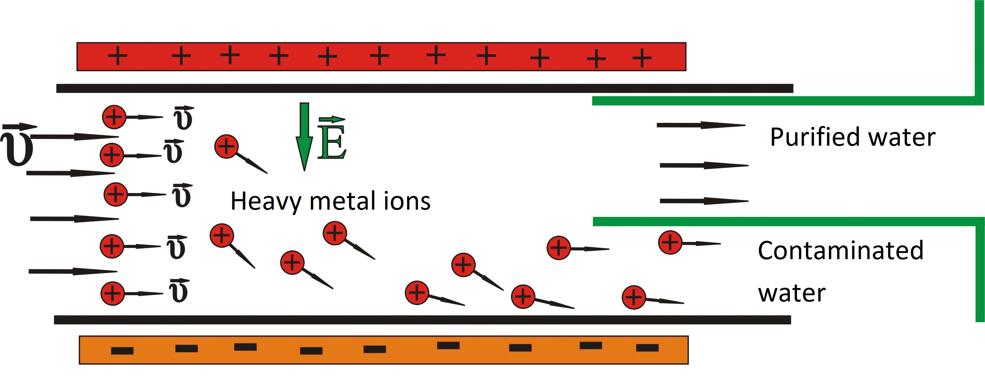
The continuous contaminated water flow in a duct is considered in an area which is under the effect of an external DC electric field (Figure 1) similar to the one detailed by Bartzis and Sarris [50,51]. The proposed configuration is thus similar to that of a usual capacitor, in which the positive heavy metal ions are attracted by the electric potential and drift to the non-conductive sidewalls of the duct. Thus, the concentration of heavy metal ions is decreased in the central area of the duct, as well as in the other sidewall area, which is a region suitable to collect the purified fluid. The effectiveness of the method is influenced by the width of the duct, the initial concentration of heavy metals, by the applied potential and the valence of the ions. An analogous configuration in nanochannels [52,53,54] within a molecular dynamics simulation showed that this method can drift salt ions successfully.

2. Materials and Methods

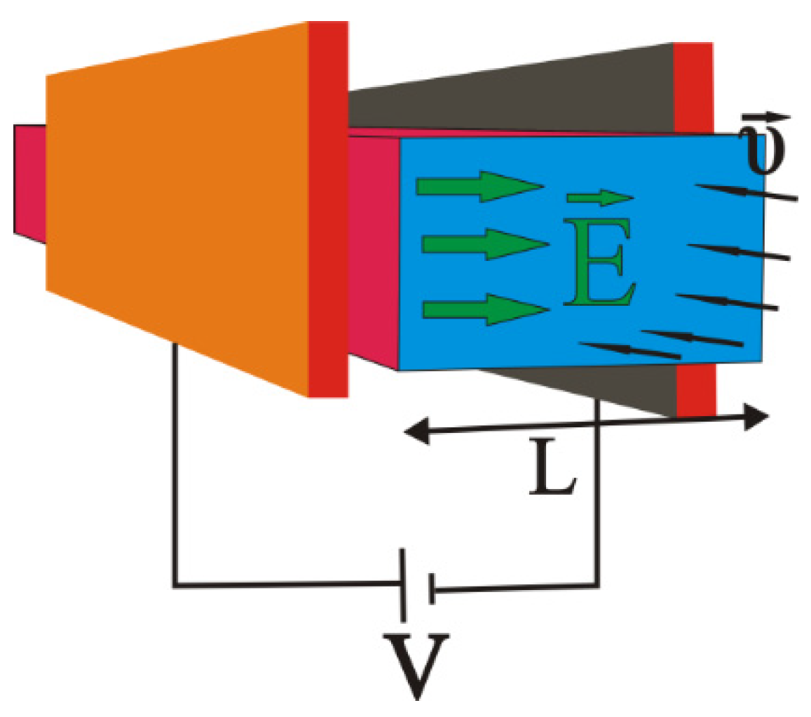
Let us assume that contaminated water contains some Cr⁺³, Cr⁺⁶, Cd⁺², Zn⁺², Fe⁺³ and/or Hg⁺² in significant concentrations. Our target is to reduce the heavy metal concentration in the outflow duct by their drift in the sidewalls of the duct. Figure 1 and Figure 2 represent the reactor that is studied in this paper. It consists of:

(1)

Two electrodes charged by a voltage V, producing between them an almost homogeneous and constant electric field with direction going from positive to negative;

(2)

An insulated duct of width L that is placed between and along the electrodes at minimal distance to ensure field uniformity. Thus, the contaminated water flows perpendicular to the electric field (Figure 1, Figure 2 and Figure 3).

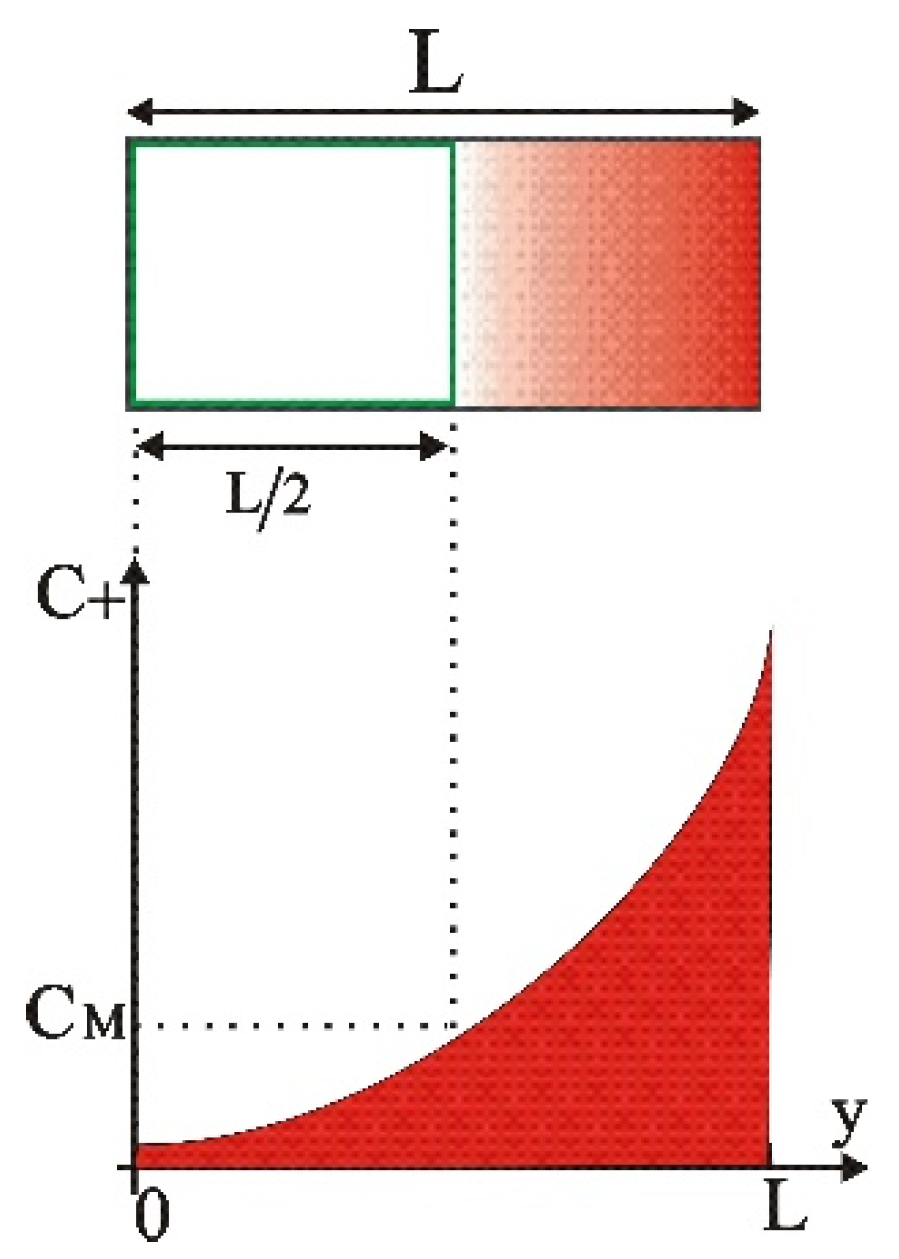
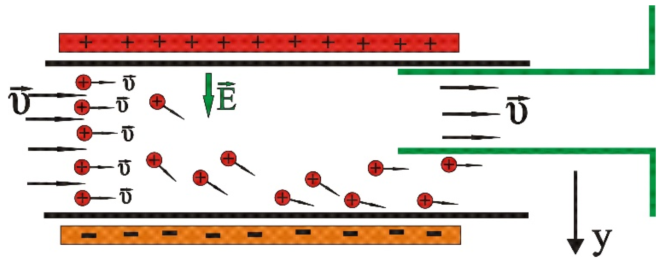
It is assumed that the water with heavy metal ions flows inside the duct. Thus, it is supposed that the solution is under the effect of the external electric field. It is considered for simplicity’s sake that the solution contains only one species of heavy metal ions. The basic idea is presented in Figure 3. Due to the electric field, the metallic ions drift towards the negative electrode of the conductor, which in Figure 3 is placed at the bottom, leaving almost ion-free water at the upper part of the duct.

Throughout the present study, water is considered as a continuous dielectric media [55,56,57,58], with electric permittivity $\mathsf{\epsilon }={\mathsf{\epsilon }}_{\mathrm{r}}{ \mathsf{\epsilon }}_0$, where ${\mathsf{\epsilon }}_{\mathrm{r}}\approx 80$ is the relative permittivity of the water and ${\mathsf{\epsilon }}_0=8.85\times {10}^{-12} \mathrm{F}/\mathrm{m}$.

3. General Study of the Final State for the Stern Model

3.1. Boundary Conditions

For the present analysis we consider the Stern model, in which the ions have finite sizes. So, the minimal distance that the ions can approach the duct’s walls is in the order of the ionic radius (further increased by hydration), and a layer that is called the compact layer is created (Stern layer), which is simulated by a Helmholtz capacitor with an effective width that is considered a constant. We use the term ‘effective’ because in this layer, due to extremely large fields, the water cannot considered a continuous medium, and if we continue to use the permittivity ε we must change its thickness ${\lambda }_s$. As usual we consider ${\lambda }_s\approx 5\dot{\mathrm{A}}$ [59,60,61]. After the compact layer, we have the diffuse layer which is simulated by a Gouy–Chapman type capacitor. These two layers form the double layer.

Before starting the study, we have to declare the boundary conditions. We consider at $y=\frac{L}{2}$ (the center of the duct) the potential to be equal to zero, $\phi (y=\frac{L}{2})=0$. In that case $\phi (0)$ is the potential at y = 0 and $-\phi (0)$ at $y=L$. Moreover, by assuming that the relation between the potential and the distance is linear inside the compact layer, we have the following:

$$\phi =\pm \phi (0)\pm {\lambda }_s\frac{\partial \phi }{\partial y} \mathrm{for} y=0,L$$

(1)

3.2. Accurate Solution for the Final State

Following the method of ref. [62] we can accurately calculate the intensity of the electric field within the compact layer and surface charge density. So according to ref. [62] we have the following:

$$\sigma =-\sqrt{8\epsilon C_{M}RT}\sinh [\frac{zF}{2RT}(\frac{\sigma {\lambda }_s}{\epsilon }+\phi (0))]$$

(2)

Or, after substituting:

$$\sigma =-3.76\times {10}^{-3}{C}_M^{\raisebox{1ex}{$1$}\!\left/ \!\raisebox{-1ex}{$2$}\right.}\sinh [z(19.34\phi (0)+13.65\sigma )] (\mathrm{S}.\mathrm{I}.)$$

(3)

where $C_M$ is the ion concentration at the middle of the duct after the electric potential application, T is the absolute temperature which is considered T = 300 K throughout this work, z is the number of overflow protons or electrons (considered positive throughout the article and equal for both positive and negative ions), $\mathrm{R}$ is the universal gas constant and F = 96,485.34 C/mol is the Faraday constant.

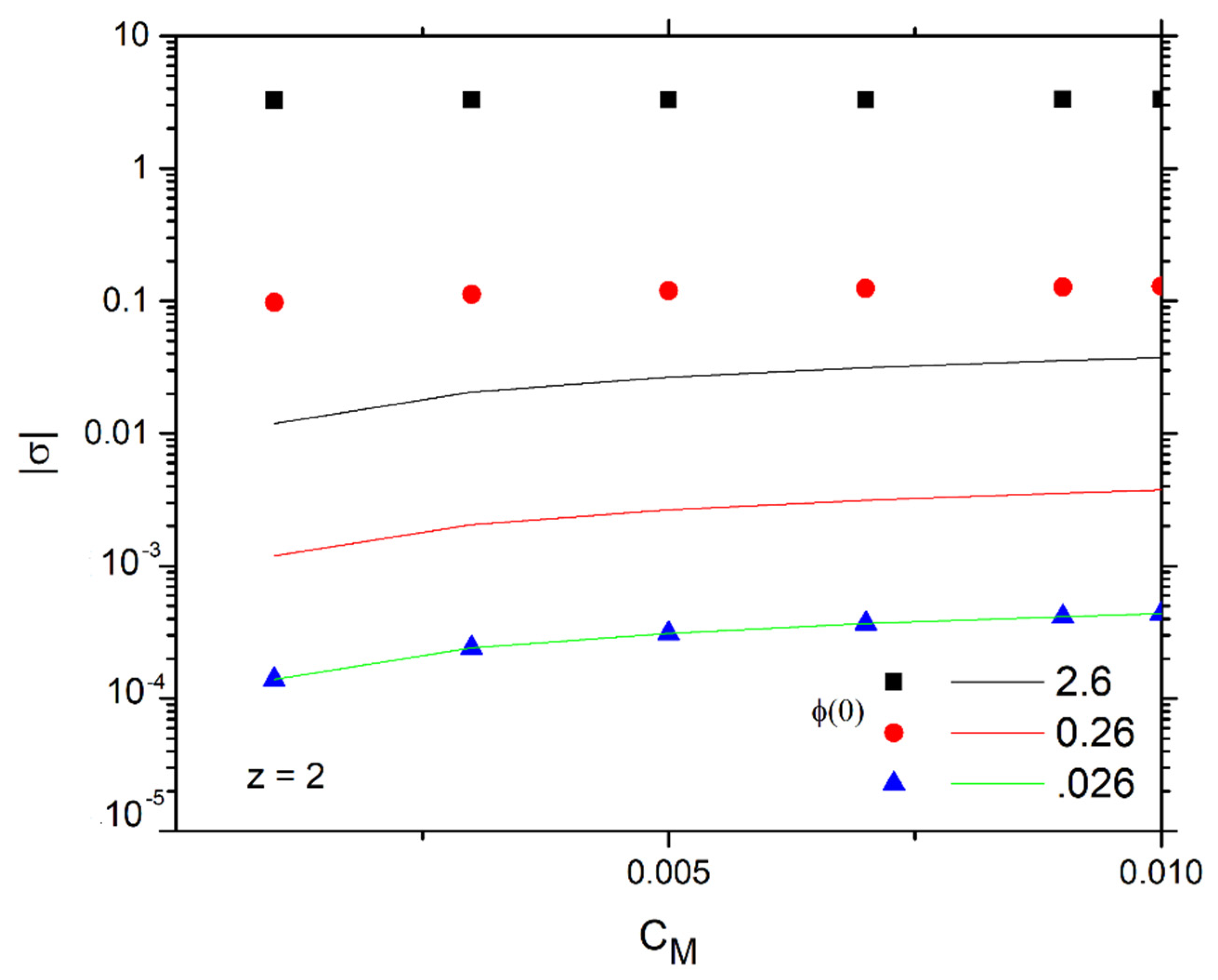
Figure 4 presents the surface charge density in its exact calculation in Equation (2) for bivalent ions as a function of $C_M$ and for various $\phi (0)$ (discrete points). It is found that $\left|\sigma \right|$ increases slightly with the increase in $C_M$, especially for low $\phi (0)$, and many orders of magnitude as $\phi (0)$ increases.

Inside the compact layer, the intensity of the electric field is given by [62]:

$${{\rm E}}_{{\lambda }_S}=-\frac{\sigma }{\epsilon }\to {{\rm E}}_{{\lambda }_S}=\sqrt{\frac{8C_{M}RT}{\epsilon }}\sinh [\frac{zF}{2RT}(-{\lambda }_s{{\rm E}}_{{\lambda }_S}+\phi (0))]$$

(4)

$$\mathrm{or}, {{\rm E}}_{{\lambda }_S}=5.31\times {10}^6{C}_M^{\raisebox{1ex}{$1$}\!\left/ \!\raisebox{-1ex}{$2$}\right.}\sinh [z(19.34\phi (0)-9.67\times {10}^{-9} {{\rm E}}_{{\lambda }_S})] (\mathrm{S}.\mathrm{I})$$

(5)

Outside the compact layer, the electric field and the potential distribution are of the form:

$$E=-\frac{\partial \phi }{\partial y}=\sqrt{\frac{8C_{M}RT}{\epsilon }}\sin \mathrm{h}(\frac{zF}{2RT}\phi )$$

(6)

$$\mathrm{or} E=-\frac{\partial \phi }{\partial y}=5.31\times {10}^6{C}_M^{\raisebox{1ex}{$1$}\!\left/ \!\raisebox{-1ex}{$2$}\right.}\sin \mathrm{h}(19.34\times z\phi )$$

(7)

$$\mathrm{where} \phi =\frac{4RT}{zF}\tan h^{-1}\{\tan h(\frac{zF{\phi }_s}{4RT})\times e^{-\kappa (y-{\lambda }_s)}\} \mathrm{for} {\lambda }_s\le y\le \raisebox{1ex}{$L$}\!\left/ \!\raisebox{-1ex}{$2$}\right.$$

(8)

$$\mathrm{and} \phi =\frac{4RT}{zF}\tan h^{-1}\{-\tan h(\frac{zF{\phi }_s}{4RT})\times e^{\kappa (y-L+{\lambda }_s)}\} \mathrm{for} \raisebox{1ex}{$L$}\!\left/ \!\raisebox{-1ex}{$2$}\right.\le y\le L-{\lambda }_s$$

(9)

where ${\lambda }_s\approx 5\dot{\mathrm{A}}$ and the potential ${\phi }_s$ at the outer Helmholtz plane (OHP) is:

$${\phi }_s=\phi (0)-{\lambda }_s\sqrt{\frac{8C_{M}RT}{\epsilon }}\sinh (\frac{zF}{2RT}{\phi }_s)$$

(10)

$$\mathrm{or} {\phi }_s=\phi (0)-2.65\times {10}^{-3}{C}_M^{\raisebox{1ex}{$1$}\!\left/ \!\raisebox{-1ex}{$2$}\right.}\sinh (19.34\times z{\phi }_s) (\mathrm{S}.\mathrm{I})$$

(11)

The total differential capacitance that is defined as $c_{tot}=\frac{\left|d\sigma \right|}{d\phi (0)}$ is given by the relation:

$$c_{tot}=\frac{\sqrt{\frac{2C_M\epsilon z^2{F}^2}{RT}}\cos \mathrm{h}(\frac{zF}{2RT}{\phi }_s)}{1+\frac{{\lambda }_s}{\epsilon }\sqrt{\frac{2C_M\epsilon z^2{F}^2}{RT}}\cos \mathrm{h}(\frac{zF}{2RT}{\phi }_s)}$$

(12)

By considering as usual that the boundary layer is constituted by two in-line capacitors, one for the compact layer (Stern layer), $c_H$, and one for the diffuse layer, $c_D$, it is found that:

$$c_H=\frac{\epsilon }{{\lambda }_s}$$

(13)

$$c_D=\sqrt{\frac{2C_M\epsilon z^2{F}^2}{RT}}\cos \mathrm{h}(\frac{zF}{2RT}{\phi }_s)$$

(14)

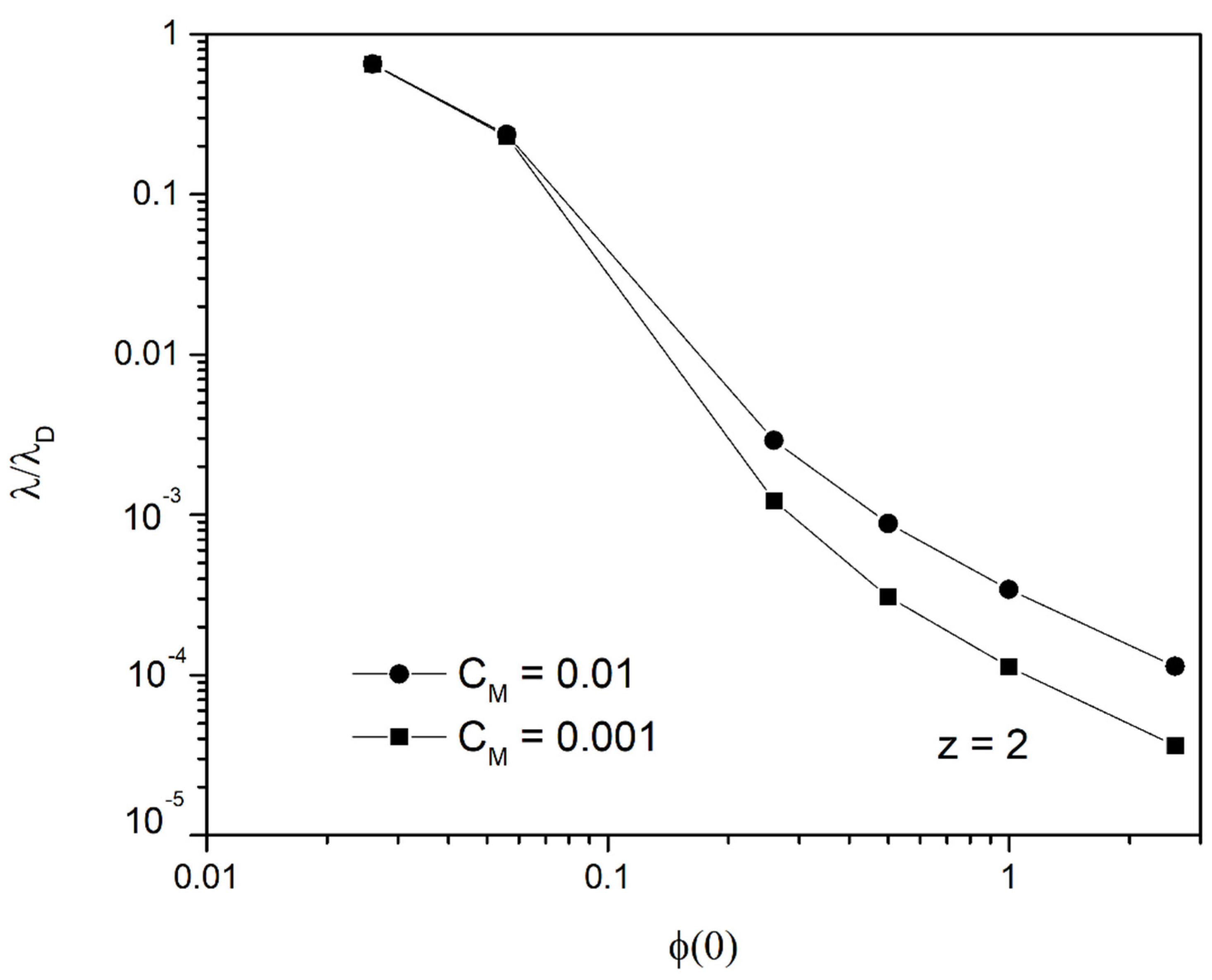
Furthermore, by substitution it is found that $c_H=1.4 \mathrm{F}/{\mathrm{m}}^2$, while $c_D$ depends on the initial concentration and the applied electric field. $c_D$ can be expressed by $c_D=\frac{\epsilon }{{\lambda }_D}\cos \mathrm{h}(\frac{zF}{2RT}{\phi }_s)$, where ${\lambda }_D={\kappa }^{-1}=\sqrt{\frac{\epsilon RT}{2z^2{C}_M{F}^2}}$ is the diffuse layer width in the linear approximation of thickness, between 50 and 150 nm for the concentrations of ions studied here. By expressing $c_D$ as $c_D=\frac{\epsilon }{\lambda }$, where $\lambda$ represents the thickness of the effective capacitor of the diffuse layer, the ration $\frac{\lambda }{{\lambda }_D}$ is then found as:

$$\frac{\lambda }{{\lambda }_D}={\left[\cos \mathrm{h}(\frac{zF}{2RT}{\phi }_s)\right]}^{-1}$$

(15)

The variation of $\frac{\lambda }{{\lambda }_D}$ is shown in Figure 5 as a function of $\phi (0)$ for two different $C_M$. As it is observed, $\frac{\lambda }{{\lambda }_D}$ is a fraction of the diffuse layer thickness in the linear regime. Thus, ions are drifted mainly in an area of thickness of the order of nm (or even smaller) for electric potentials $\phi (0)$ of interest, i.e., 0.26 V and more, leaving most of the duct free of heavy metals.

Moreover, the ion concentration distribution along the duct is considered to follow the Boltzmann distribution, which gives for the case of the negative ions (which are exactly symmetrical at the opposite pole of the positive ions) the distribution outside of the diffuse layers ${\lambda }_s$ at the two sidewalls of the duct:

$$C_{-}=C_M{e}^{+\frac{zF}{RT}\phi }$$

(16)

where $\phi$ is given by the relations (8) and (9).

Considering that $C_M$ is the ion concentration at the middle of the duct after the electric potential application, the uniform initial concentration can be estimated as:

$$C_{bef}=\frac{C_M{\int }_{{\lambda }_s}^{L-{\lambda }_s}{e}^{+\frac{zF}{RT}\phi }dy}{L}$$

(17)

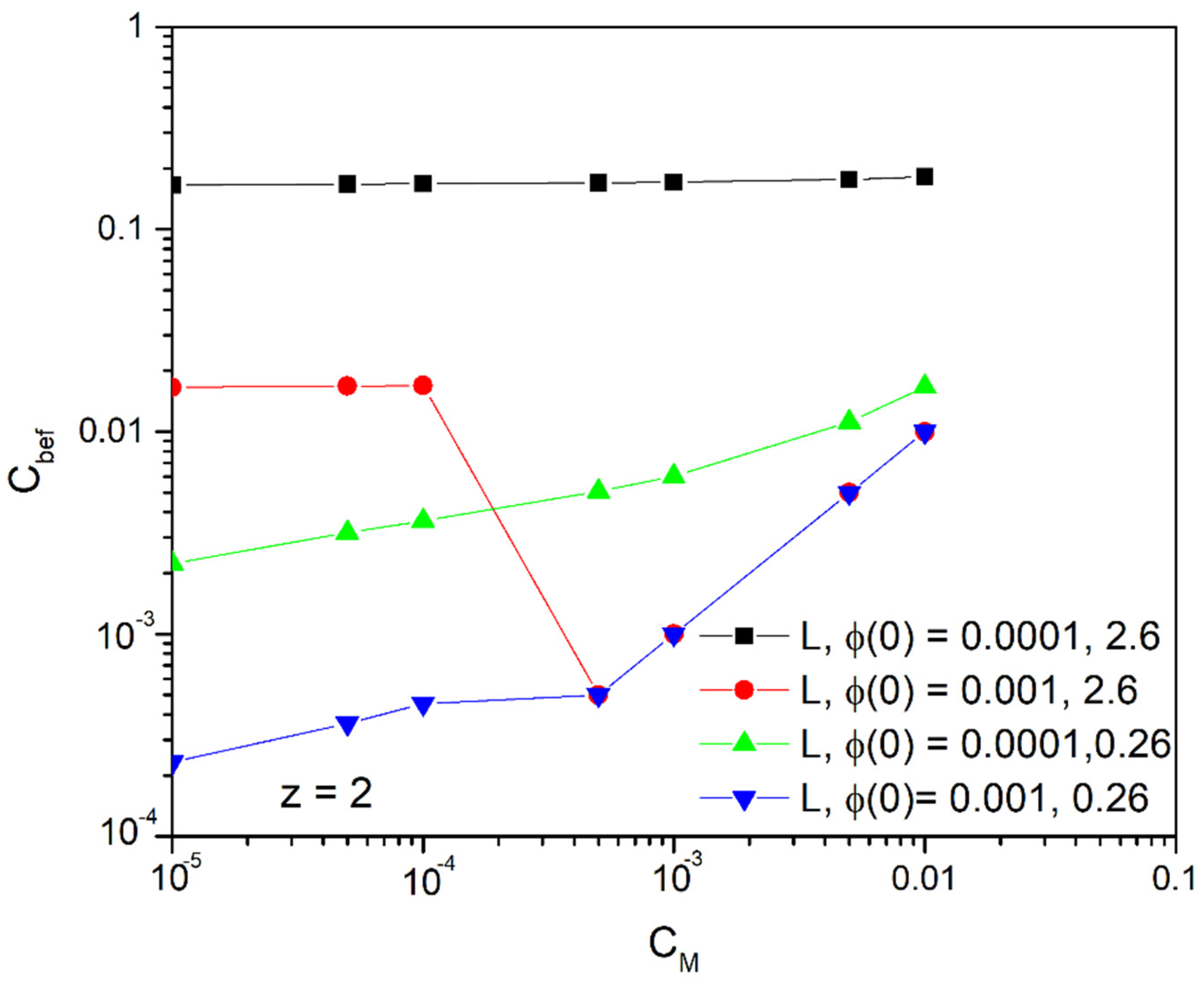
Figure 6 gives an initial idea of the regimes in which this method works efficiently. In general, $C_{bef}$ should be higher than the ion concentration in middle of the duct after the electric potential application $C_M$. As it is observed, for bivalent ions and for ducts of widths $L=0.0001 \mathrm{m}$ and smaller, the method is applied (i.e., we have a decrease in the concentration of the main volume of the solution) when we want to achieve concentrations $C_M$ below 0.01 mol/m³ and for the two potentials $\phi (0)=0.26 \mathrm{V}$ and $\phi (0)=2.6 \mathrm{V}$ (green and black lines, respectively).

For duct widths of $L=0.001 \mathrm{m},$ the method is applied in the case of the potential $\phi (0)=0.26 \mathrm{V}$ (blue line) when we want to achieve concentrations $C_M$ below 0.001 mol/m³. The case in which $\phi (0)=2.6 \mathrm{V}$, $L=0.001 \mathrm{m},$ corresponding to the red line, is discontinuous and we consider that it is reliable only in the part where it coincides with the blue line. We must emphasize here that as the potential grows above $\phi (0)=0.26 \mathrm{V}$, the steric effects become more and more important, as we will explore later, and the above model diverges more and more. Nevertheless, the results have their qualitative significance.

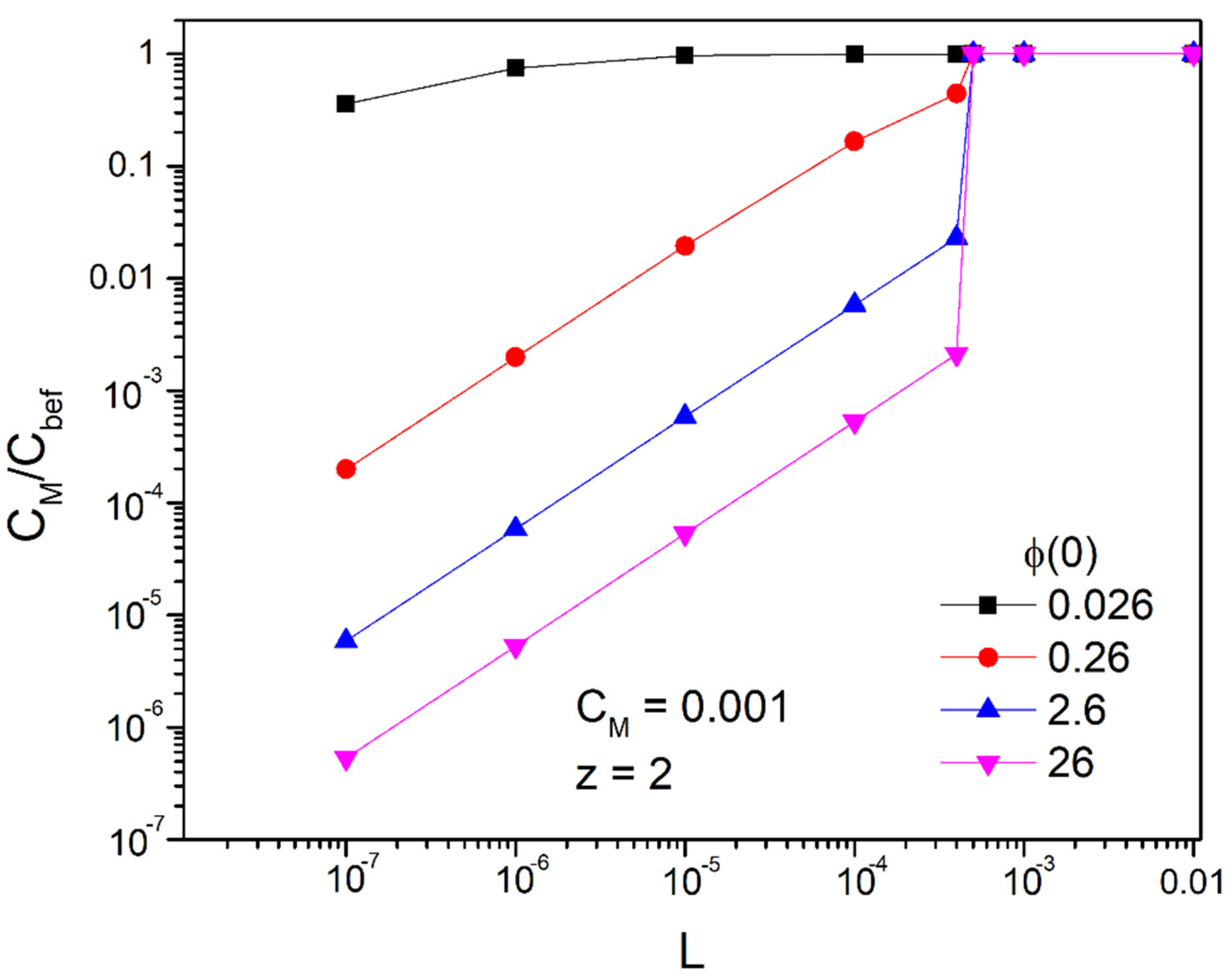
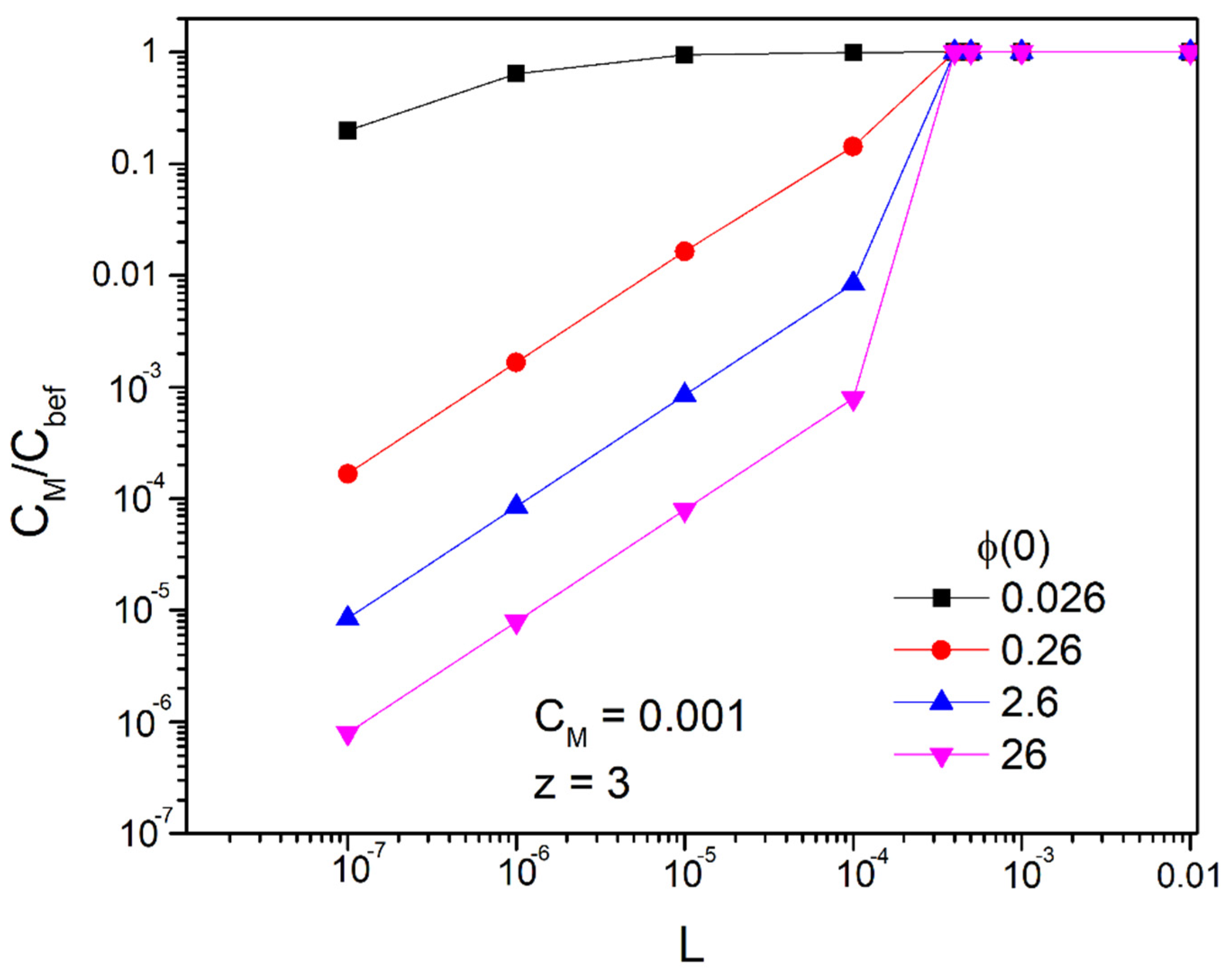
According to the above, we are led to the conclusion that if we want to achieve concentrations below $C_M=0.001 \mathrm{mol}/{\mathrm{m}}^3,$ as is the limit based on the international literature [1] for hexavalent chromium, we can achieve it by using ducts with a width of L < 0.001 m (in fact smaller than 4 × 10⁻⁴ m, as we will see below). In Figure 7 and Figure 8 we represent the fraction

$$\frac{C_M}{C_{bef}}=\frac{L}{{\int }_{{\lambda }_s}^{L-{\lambda }_s}{e}^{+\frac{zF}{RT}\phi }dy}$$

(18)

as a function of the width of the duct L for the bivalent and trivalent ions, respectively, and for the desired concentration, $C_M=0.001 \mathrm{mol}/{\mathrm{m}}^3$.That is, keeping constant the numerator of the fraction which represents the desired concentration, $C_M=0.001 \mathrm{mol}/{\mathrm{m}}^3$, we find the ratio of this with the concentration before the application of the field, $C_{bef}$. Therefore, the smaller the ratio, the better results we have

We observe that for potentials $\phi (0)$ greater than or equal to 0.26 V and for widths up to 1 mm there is an extremely large decrease in the concentration of the bulk of the solution. Of course, as expected, with the reduction in the width, the ratio $\frac{C_M}{C_{bef}}$ becomes smaller. The critical amplitude at which there is no significant decrease in the concentration of the bulk of the solution after application of the field is between $L=0.0001 \mathrm{m}$ and $L=0.001 \mathrm{m}$. For z = 2 it is approximately in $L=4\times {10}^{-4} \mathrm{m}$ and for z = 3 in $L=2\times {10}^{-4} \mathrm{m}$. Even for small magnitudes of the applied potentials of the order $\phi (0)=0.26 \mathrm{V},$ we have a reduction in concentration by 90% with a width $L=0.0001 \mathrm{m}$. For an order of magnitude higher potential, it reaches 99%. However, as we will see below when potential $\phi (0)$ is greater than 0.26 V, we can only draw qualitative conclusions because steric effects are then involved. Nevertheless, we see an extremely large reduction in the concentration of heavy metals in the main volume of the solution.

3.3. Validity of the Model

There are a few limitations posed by the fact that ions have finite dimensions. Let us consider that the diameter of the ion is of the order ${\mathrm{a}}_0=1\dot{\mathrm{A}}$. If we include the solvation shell, its diameter becomes $\mathrm{a}=3\dot{\mathrm{A}}$. However, if we also take into account the ion, ion correlations will effectively increase to $\mathrm{a}=7\dot{\mathrm{A}}$, equal to the Bjerrum length. Lastly, we should mention the solvent effect. It is generally believed that in the Stern layer, the water dipoles are so highly aligned that the effective permittivity drops from $80{\epsilon }_0$ to $5{\epsilon }_0$. In applied large voltages, this probably extends to the diffuse layer by changing the Bjerrum length perhaps up to 10 nm. By taking into account a middle value, we then consider that $\mathrm{a}=10\dot{\mathrm{A}}$. The maximum concentration is reached where the Stern layer (compact layer) ends and the diffuse layer begins. This cannot be greater than [63]:

$$C_{max}=\frac{1}{N_A{a}^3}=1660\raisebox{1ex}{$\mathrm{mol}$}\!\left/ \!\raisebox{-1ex}{${\mathrm{m}}^3$}\right.$$

The relationship that connects it with the ${\phi }_s$ that prevails at this point is:

$$C_{max}=C_M{e}^{+\frac{zF}{RT}{\phi }_s}$$

Thus:

$${\phi }_s=\frac{RT}{zF}\ln (\frac{C_{max}}{C_M}) |$$

(19)

where the corresponding $\phi (0)$ is calculated from Equation (10). Replacing the values of the parameters, we find that for $z=2$ and $C_M=0.001 \mathrm{mol}/{\mathrm{m}}^3$ is $\phi (0)=0.24 \mathrm{V}$, while for $z=3$ and for the same $C_M$, it is $\phi (0)=0.17 \mathrm{V}$. We cannot claim that the above values are more than indicative because of the approximations with which they were extracted. However, again, the closer we approach them, the more the density increases in OHP and the less the dilute solution approximation is valid, which is necessary for the Boltzmann distribution to apply. So, referring to the previous analysis, for potentials above approximately 0.26 V, the results can only be considered qualitatively. However, given the extremely large reduction we achieve in the concentration of heavy metals even with potentials $\phi (0)$ of the order of 0.26 V as already mentioned, the further increase in the potential can only bring about an increase in performance.

4. PNP Equations for the Stern Model

Following the methodology of ref. [62], the Poisson–Nernst–Plank equations (PNP) for the ionic flux and the charge density read as:

$$\frac{\partial C_{\pm }}{\partial t}=-\frac{\partial }{\partial y}(J_{\pm })=-\frac{\partial }{\partial y}(\mp C_{\pm }ze\mu \frac{\partial \phi }{\partial y}-D\frac{\partial C_{\pm }}{\partial y})$$

(20)

$$\frac{{\partial }^2\phi }{\partial y^2}=-\frac{\rho }{\epsilon }\to \frac{{\partial }^2\phi }{\partial y^2}=-\frac{zF(C_{+}-C_{-})}{\epsilon }$$

(21)

where $C_{\pm }$ and $J_{\pm }$ are the concentration and ionic flux of the positive and negative ions, respectively,$\mathrm{D}=\mu \mathrm{kT}$ is the diffusion coefficient of the ions,$\mu$ is their mobility (we considered in Εquation (20) that both positive and negative ions have the same mobility ${\mu }_{+}={\mu }_{-}=\mu$, and thus the same diffusion coefficient $D_{+}=D_{-}=D$). Additionally, $\mathrm{k}\equiv \frac{\mathrm{R}}{{\mathrm{N}}_{\mathrm{A}}}$ is the Boltzmann constant and the mobility is related with the dynamic viscosity $\mathsf{\nu }$ and with the effective radius of the ions $\mathrm{r}$ by the relation $\mu \equiv \frac{1}{6\mathsf{\pi }\mathsf{\nu }\mathrm{r}}$. Moreover, φ is the potential of the fluid’s bulk,${ \mathsf{{\rm N}}}_{\mathrm{A}}$ is the Avogadro constant, and the absolute temperature is considered T = 300 K throughout this work as we have already mentioned. In the above Equation (20), the electric field intensity has been substituted by $\mathsf{{\rm E}}=-\frac{\partial \mathsf{\phi }}{\partial \mathrm{y}}$. Additionally z is the number of overflow protons or electrons (considered positive throughout the article and equal for both positive and negative ions) and $\mathrm{e}=1.6\times {10}^{-19}\mathrm{Cb}$. So the charge density has the form:

$$\mathsf{\rho }={\mathrm{C}}_{+}\mathrm{zF}-{\mathrm{C}}_{-}\mathrm{zF}=\mathrm{zF}({\mathrm{C}}_{+}-{\mathrm{C}}_{-})$$

(22)

where F = 96,485.34 C/mol is the Faraday constant.

Since no charge is transferred between the electrodes, a non-Faradaic procedure [61] is performed, and the ionic fluxes and the current density are given by:

$$J_{\pm }=\mp C_{\pm }ze\mu \frac{\partial \phi }{\partial y}-D\frac{\partial C_{\pm }}{\partial y}=0 \mathrm{for} y=0,L$$

(23)

$$i=ze{N}_A(J_{+}-J_{-})=0 \mathrm{for} y=0,L$$

(24)

Moreover, uniform ion distribution $C_{+}^{bef}=C_{-}^{bef}=C^{bef}$ is initially assumed and the zero potential is at t < 0.

4.1. Linearized Solution of the PNP Equations

The linear approximation in the solution of PNP Equations (20) and (21) is discussed in ref. [62], in which their validity in the fluid’s bulk was proven because of the weak ion drift towards the duct and the small concentration shift in the y-axis. The linear approximation can also cover the diffuse layer in the case of [62]:

$$\left|z\frac{\mathrm{F}}{\mathrm{RT}}\mathsf{\phi }\right|<1 \mathrm{or} z\mathsf{\phi }(0)\le 0.026 \mathrm{V}$$

(25)

$$\mathrm{So} \mathrm{we} \mathrm{have} \frac{1}{\mathrm{D}}\frac{\partial \mathsf{\rho }}{\partial \mathrm{t}}=\frac{{\partial }^2\mathsf{\rho }}{\partial {\mathrm{y}}^2}-{\mathsf{\kappa }}^2\mathsf{\rho }$$

(26)

$$\mathrm{where}, \mathsf{\kappa }=\sqrt{\frac{2{\mathrm{z}}^2{\mathrm{C}}_{\mathrm{M}}{\mathrm{F}}^2}{\mathsf{\epsilon }\mathrm{RT}}}$$

(27)

The solution of the above Equation of Equations gives [62]:

$$\mathsf{\rho }=\alpha \sinh \left(\mathsf{\kappa }\left(\mathrm{y}-\frac{\mathrm{L}}{2}\right)\right)(1-e^{-\frac{t}{\tau }})$$

(28)

$$\frac{\partial \mathsf{\phi }}{\partial \mathrm{y}}=-\frac{\mathsf{\alpha }}{\mathsf{\epsilon }\mathsf{\kappa }}\cosh \left(\mathsf{\kappa }\left(\mathrm{y}-\frac{\mathrm{L}}{2}\right)\right)\left(1-e^{-\frac{t}{\tau }}\right)-\alpha \frac{1}{\tau }{e}^{-\frac{t}{\tau }}\frac{\cosh \left(\mathsf{\kappa }\frac{\mathrm{L}}{2}\right)}{\epsilon D{\kappa }^3}$$

(29)

$$\mathsf{\phi }=-\alpha \frac{\sinh \left[\mathsf{\kappa }\left(\mathrm{y}-\frac{\mathrm{L}}{2}\right)\right]}{{\mathsf{\epsilon }\mathsf{\kappa }}^2} \left(1-e^{-\frac{t}{\tau }}\right)-\mathsf{\alpha }\frac{1}{\tau }{e}^{-\frac{t}{\tau }} \frac{\left(\mathrm{y}-\frac{\mathrm{L}}{2}\right)}{\mathsf{\epsilon }\mathrm{D}{\kappa }^3}\cosh \left(\mathsf{\kappa }\frac{\mathrm{L}}{2}\right)$$

(30)

$$\mathrm{where}, \alpha =\frac{\mathsf{\phi }\left(0\right){\mathsf{\epsilon }\mathsf{\kappa }}^2}{\cosh \left(\mathsf{\kappa }\frac{\mathrm{L}}{2}\right)\left({\mathsf{\lambda }}_{\mathrm{s}}\mathsf{\kappa }+\tanh \left(\mathsf{\kappa }\frac{\mathrm{L}}{2}\right)\right)}$$

(31)

$$\tau =\frac{\mathrm{L}\left(1+\frac{2{\mathsf{\lambda }}_{\mathrm{s}}}{\mathrm{L}}\right)}{2\mathrm{D}\mathsf{\kappa }\left({\mathsf{\lambda }}_{\mathrm{s}}\mathsf{\kappa }+\tanh \left(\mathsf{\kappa }\frac{\mathrm{L}}{2}\right)\right)}$$

(32)

By using the definition of charge density, the ion concentration distributions can be estimated as:

$$C_{+}=C_M+\frac{\alpha \sinh \left(\mathsf{\kappa }\left(\mathrm{y}-\frac{\mathrm{L}}{2}\right)\right)}{2zF}(1-e^{-\frac{t}{\tau }})$$

(33)

$$C_{-}=C_M-\frac{\alpha \sinh \left(\mathsf{\kappa }\left(\mathrm{y}-\frac{\mathrm{L}}{2}\right)\right)}{2zF}(1-e^{-\frac{t}{\tau }})$$

(34)

If the duct has width $L\ge {10}^{-5} \mathrm{m}$, and since ${\lambda }_s~1-10\dot{\mathrm{A}},$ it is found that the rate $\frac{{\lambda }_s}{L}\le {10}^{-4}$, and thus may be considered negligible. Moreover, for such duct width and since $\kappa ~{10}^6{\mathrm{m}}^{-1}$, it can also be considered that $\tanh (\mathsf{\kappa }\frac{\mathrm{L}}{2})\approx 1$. Introducing these simplifications, we have the following:

$$\tau =\frac{\mathrm{L}}{2\mathrm{D}\mathsf{\kappa }({\mathsf{\lambda }}_{\mathrm{s}}\mathsf{\kappa }+1)}$$

(35)

$$\alpha =\frac{\mathsf{\phi }(0){\mathsf{\epsilon }\mathsf{\kappa }}^2}{\cosh (\mathsf{\kappa }\frac{\mathrm{L}}{2})({\mathsf{\lambda }}_{\mathrm{s}}\mathsf{\kappa }+1)}$$

(36)

4.2. Long Time Behavior of the Linearized Approximation

In this paragraph we will study the above magnitudes of Equations (28)–(30), (33) and (34) in the final equilibrium state as the time increases to infinity, and then $(1-e^{-\frac{t}{\tau }})\to 1$ and $e^{-\frac{t}{\tau }}\to 0$. So the above magnitudes have equilibrium equations as follows:

$$\mathsf{\rho }=\alpha \sinh \left(\mathsf{\kappa }\left(\mathrm{y}-\frac{\mathrm{L}}{2}\right)\right)$$

(37)

$$\frac{\partial \mathsf{\phi }}{\partial \mathrm{y}}=-\frac{\mathsf{\alpha }}{\mathsf{\epsilon }\mathsf{\kappa }}\cosh \left(\mathsf{\kappa }\left(\mathrm{y}-\frac{\mathrm{L}}{2}\right)\right)$$

(38)

$$\mathsf{\phi }=-\alpha \frac{\sinh \left[\mathsf{\kappa }\left(\mathrm{y}-\frac{\mathrm{L}}{2}\right)\right]}{{\mathsf{\epsilon }\mathsf{\kappa }}^2}$$

(39)

$$C_{+}=C_M+\frac{\alpha \sinh \left(\mathsf{\kappa }\left(\mathrm{y}-\frac{\mathrm{L}}{2}\right)\right)}{2zF}$$

(40)

$$C_{-}=C_M-\frac{\alpha \sinh \left(\mathsf{\kappa }\left(\mathrm{y}-\frac{\mathrm{L}}{2}\right)\right)}{2zF}$$

(41)

The above results (which were obtained on the basis of the linear approach) should be compatible with those found in Section 3.2. To verify this, we will calculate the surface charge density (in $\mathrm{C}/{\mathrm{m}}^2$). Following the methodology of ref. [62] we have for the surface charge density the following:

$$\left|{\sigma }_l\right|=\phi (0)\frac{\epsilon }{({\lambda }_S+{\kappa }^{-1})}$$

(42)

Figure 4 shows the variation in the graph of $\left|{\sigma }_l\right|$ as a function of the concentration $C_M$ for bivalent ions but also for different externally applied potentials $\phi (0)$ (solid lines). In the same plot with the discrete points, the surface charge density is represented for the same potentials using the exact calculations of Equation (2) or (3). We observe the full identification of the results for potentials $\phi (0)$ up to 0.026 V (as should be the case for the linear approach to apply) and their gradual deviation for larger potentials. Specifically, the predictions of the exact calculation method give higher surface charge density values for potentials $\phi (0)$ from 0.26 V (two orders of magnitude difference) and above, with the difference increasing as the potential increases, as expected.

4.3. Time Prediction with the Linear Approach

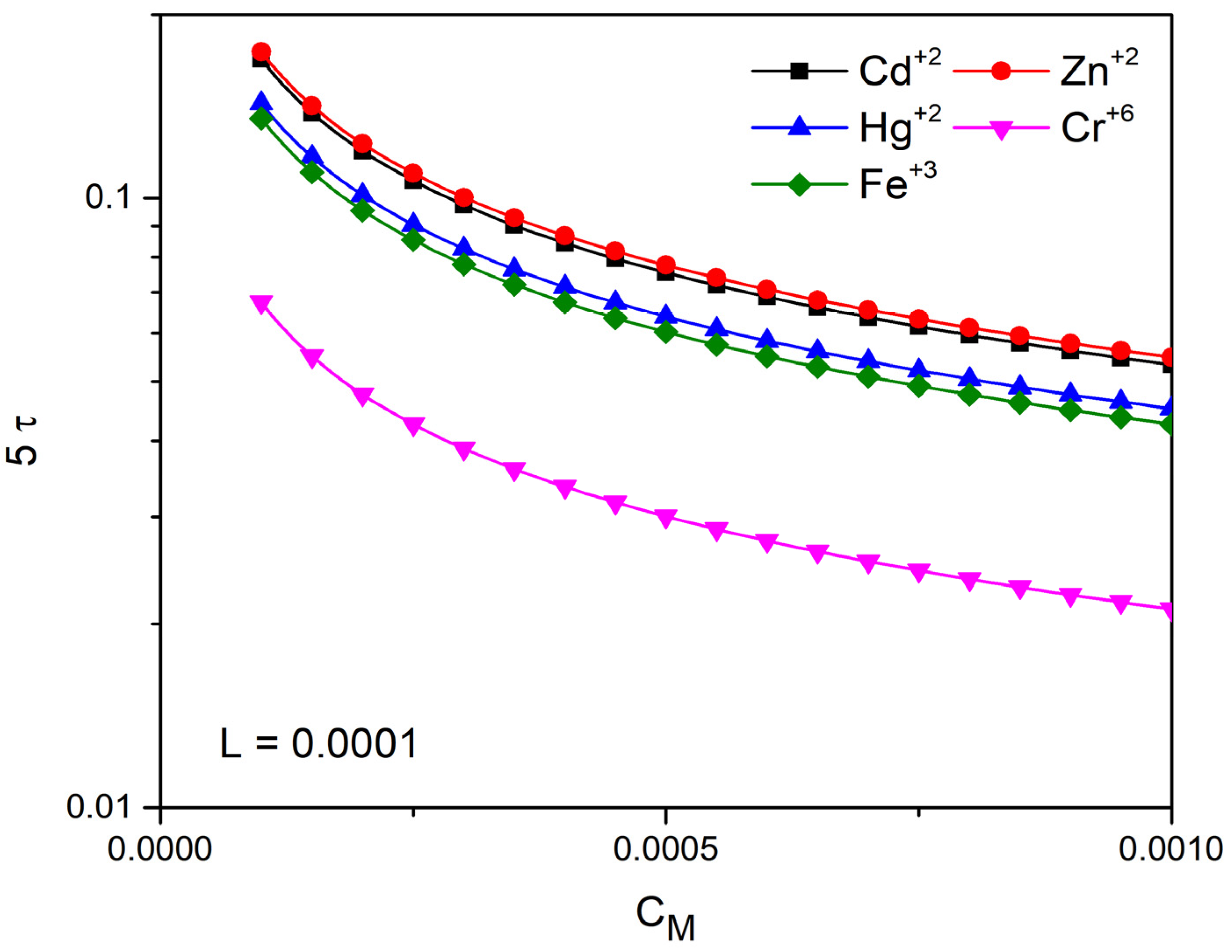
The linear solution above is equivalent to a RC circuit with time constant $\tau$, ref. [62]. Thus, according to the electric circuit theory, the equilibrium will be reached at $5\tau$. In Figure 9 and Figure 10, we plot 5τ versus concentration for characteristic ions with z = 2 and z = 3 with the following diffusion coefficients.

$$\begin{gathered} D_{C{d}^{+2}}=0.72\times {10}^{-9} {\mathrm{m}}^2/\mathrm{s} \\ {D}_{Z{n}^{+2}}=0.70\times {10}^{-9} {\mathrm{m}}^2/\mathrm{s} \\ {D}_{H{g}^{+2}}=0.85\times {10}^{-9} {\mathrm{m}}^2/\mathrm{s} \\ {D}_{C{r}^{+6}}=0.60\times {10}^{-9} {\mathrm{m}}^2/\mathrm{s} \\ {D}_{F{e}^{+3}}=0.60\times {10}^{-9} {\mathrm{m}}^2/\mathrm{s} \end{gathered}$$

while in the calculations it is assumed that ${\mathsf{\lambda }}_{\mathrm{s}}\approx 5\dot{\mathrm{A}}$.

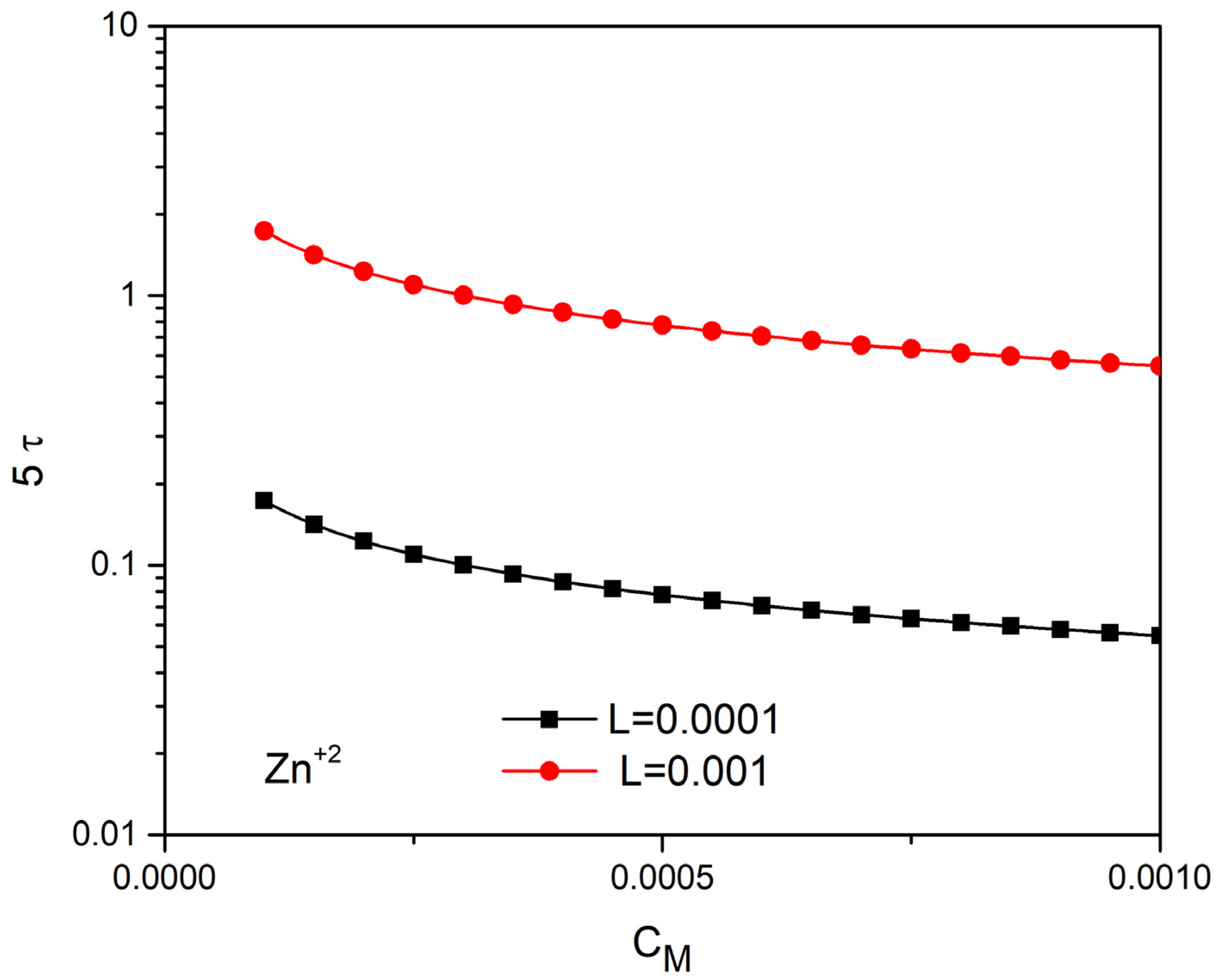
In Figure 9, keeping the thickness of the tube constant $L=0.0001 \mathrm{m}$, we examine the time of completion of the phenomenon as a function of the ion concentration and for five different ions. We observe that the higher valence ions complete their movement in less time. We notice that increasing the concentration reduces the time of completion. The completion time is also reduced when the thickness of the conductor decreases (Figure 10).

Of course, the above analysis for the time of completion of the phenomenon applies, assuming the aforementioned linear approach applies when $\left|z\frac{\mathrm{F}}{\mathrm{RT}}\mathsf{\phi }\right|<1$ or $z\mathsf{\phi }(0)\le 0.026 \mathrm{V}$. Applying larger external voltages, we have every reason to believe that the phenomenon will be completed in even shorter times, i.e., below sec for widths of the order of mm while below a tenth of the sec for widths of about a tenth of mm.

5. Conclusions

In our opinion, the present results are very encouraging for the application of the above method for the decontamination of heavy metals from water solutions. For small pipeline widths below 1 mm and even for small applied potentials $\phi (0)$ of the order of 0.26 V, we have a 90% reduction in the concentration of heavy metals in the main volume of the solution and for target concentrations of 0.001 mol/m³. That is, we can have acceptable concentration values of heavy metals with potentially ten times more contaminated solutions, which makes the method promising for practical applications.

Generally speaking, the above method can be applicable for all ions with proper potentials and duct widths.

References

- Bakarat, Μ.A. New trents in removing heavy metals from industrial wastewater. Arab. J. Chem. 2011, 4, 361–377. [Google Scholar] [CrossRef] [Green Version]
- Babel, S.; Kurniawan, T.A. Low-cost adsorbents for heavy metals uptake from contaminated water: A review. J. Hazard. Mater. 2003, B97, 219–243. [Google Scholar] [CrossRef]
- Babel, S.; Kurniawan, T.A. Various treatment technologies to remove arsenic and mercury from contaminated groundwater: An overview. In Proceedings of the First International Symposium on Southeast Asian Water Environment, Bangkok, Thailand, 24–25 October 2003; pp. 433–440. [Google Scholar]
- Babel, S.; Kurniawan, T.A. Cr (VI) removal from synthetic wastewater using coconut shell charcoal and commercial activated carbon modified with oxidizing agents and/or chitosan. Chemosphere 2004, 54, 951–967. [Google Scholar] [CrossRef] [PubMed]
- Alves-Junior, C.; Rodrigues-Junior, F.E.; Vitoriano, J.O.; Barauna, J.B.F.O. Investigating the Influence of the Pulsed Corona Discharge over Hypersaline Water. Mater. Res. 2021, 24, e20210261. [Google Scholar] [CrossRef]
- Abdelmoaty, H.M.; Mahgoub, A.U.; Abdeldayem, A.W. Performance analysis of salt reduction levels in indirect freeze desalination system with and without magnetic field exposure. Desalination 2021, 508, 115021. [Google Scholar] [CrossRef]
- Wang, L.K.; Vaccari, D.A.; Li, Y.; Shammas, N.K. Chemical Precipitation Physicochemical Treatment Processes; Humana Press: Totowa, NJ, USA, 2004; Volume 3, pp. 141–198. [Google Scholar]
- Aziz, H.A.; Adlan, M.N.; Ariffin, K.S. Heavy metals (Cd, Pb, Zn, Ni, Cu and Cr (III)) removal from water in Malaysia: Post treatment by high quality limestone. Bioresour. Technol. 2008, 99, 1578–1583. [Google Scholar] [CrossRef] [PubMed]
- Igwe, J.C.; Ogunewe, D.N.; Abia, A.A. Competitive adsorption of Zn (II), Cd (II) and Pb(II) ions from aqueous and non-aqueous solution by maize cob and husk. Afr. J. Biotechnol. 2005, 4, 1113–1116. [Google Scholar]
- Ajmal, M.; Rao, R.; Ahmad, R.; Ahmad, J. Adsorption studies on Citrus reticulata (fruit peel of orange) removal and recovery of Ni (II) from electroplating wastewater. J. Hazard. Mater. 2000, 79, 117–131. [Google Scholar] [CrossRef]
- Bansode, P.R.; Losso, J.N.; Marshall, W.E.; Rao, R.M.; Portier, R.J. Adsorption of metal ions by pecan shell-based granular activated carbons. Bioresour. Technol. 2003, 89, 115–119. [Google Scholar] [CrossRef]
- Tang, P.; Lee, C.K.; Low, K.S.; Zainal, Z. Sorption of Cr (VI) and Cu(II) in aqueous solution by ethylenediamine modified rice hull. Environ. Technol. 2003, 24, 1243–1251. [Google Scholar] [CrossRef] [PubMed]
- Fenga, D.; Aldrich, C. Adsorption of heavy metals by biomaterials derived from the marine alga Ecklonia maxima. Hydrometallurgy 2004, 73, 1–10. [Google Scholar] [CrossRef]
- Uysal, M.; Ar, I. Removal of Cr (VI) from industrial wastewaters by adsorption: Part I: Determination of optimum conditions. J. Hazard. Mater. 2007, 149, 482–491. [Google Scholar] [CrossRef] [PubMed]
- Deliyanni, E.A.; Peleka, E.N.; Matis, K.A. Removal of zinc ion from water by sorption onto iron-based nanoadsorbent. J. Hazard. Mater. 2007, 141, 176–184. [Google Scholar] [CrossRef] [PubMed]
- Barakat, M.A. Adsorption behavior of copper and cyanide ions at TiO2–solution interface. J. Colloid Interface Sci. 2005, 291, 345–352. [Google Scholar] [CrossRef]
- Bose, P.; Bose, M.A.; Kumar, S. Critical evaluation of treatment strategies involving adsorption and chelation for wastewater containing copper, zinc, and cyanide. Adv. Environ. Res. 2002, 7, 179–195. [Google Scholar] [CrossRef]
- Barakat, M.A. Adsorption of heavy metals from aqueous solutions on synthetic zeolite. Res. J. Environ. Sci. 2008, 2, 13–22. [Google Scholar]
- Solenera, M.; Tunalib, S.; Ozcan, A.S.; Ozcanc, A.; Gedikbey, T. Adsorption characteristics of lead (II) ions onto the clay/poly(methoxyethyl) acrylamide (PMEA) composite from aqueous solutions. Desalination 2008, 223, 308–322. [Google Scholar] [CrossRef]
- Crini, G. Recent developments in polysaccharide-based materials used as adsorbents in wastewater treatment. Prog. Polym. Sci. 2005, 30, 38–70. [Google Scholar] [CrossRef]
- Lee, S.T.; Mi, F.L.; Shen, Y.J.; Shyu, S.S. Equilibrium and kinetic studies of copper (II) ion uptake by chitosan–tripolyphosphate chelating resin. Polymer 2001, 42, 1879–1892. [Google Scholar] [CrossRef]
- Kurniawan, T.A.; Chan, G.Y.S.; Lo, W.H.; Babel, S. Physicochemical treatment techniques for wastewater laden with heavy metals. Chem. Eng. J. 2006, 118, 83–98. [Google Scholar] [CrossRef]
- Vigneswaran, S.; Ngo, H.H.; Chaudhary, D.S.; Hung, Y.T. Physico-chemical treatment processes for water reuse. In Physicochemical Treatment Processes; Humana Press: Totowa, NJ, USA, 2004; Volume 3, pp. 635–676. [Google Scholar]
- Juang, R.S.; Shiau, R.C. Metal removal from aqueous solutions using chitosan-enhanced membrane filtration. J. Membr. Sci. 2000, 165, 159–167. [Google Scholar] [CrossRef]
- Saffaj, N.; Loukil, H.; Younssi, S.A.; Albizane, A.; Bouhria, M.; Persin, M.; Larbot, A. Filtration of solution containing heavy metals and dyes by means of ultrafiltration membranes deposited on support made of Morrocan clay. Desalination 2004, 168, 301–306. [Google Scholar] [CrossRef]
- Cohen-Tanugi, D.; Grossman, J. Water Desalination across Nanoporous Graphene. Nano Lett. 2012, 12, 3602–3608. [Google Scholar] [CrossRef] [PubMed]
- Lv, J.; Wang, K.Y.; Chung, T.S. Investigation of amphoteric polybenzimidazole (PBI) nanofiltration hollow fiber membrane for both cation and anions removal. J. Membr. Sci. 2008, 310, 557–566. [Google Scholar] [CrossRef]
- Khedr, M.G. Membrane methods in tailoring simpler, more efficient, and cost effective wastewater treatment alternatives. Desalination 2008, 222, 135–145. [Google Scholar] [CrossRef]
- Abu Qdaisa, H.; Moussab, H. Removal of heavy metals from wastewater by membrane processes: A comparative study. Desalination 2004, 164, 105–110. [Google Scholar] [CrossRef]
- Telles, I.; Levin, Y.; Santos, A. Reversal of Electroosmotic Flow in Charged Nanopores with Multivalent Electrolyte. Langmuir 2022, 38, 3817–3823. [Google Scholar] [CrossRef] [PubMed]
- Skubal, L.R.; Meshkov, N.K.; Rajh, T.; Thurnauer, M. Cadmium removal from water using thiolactic acid-modified titanium dioxide nanoparticles. J. Photochem. Photobiol. A Chem. 2002, 148, 393–397. [Google Scholar] [CrossRef]
- Herrmann, J.M. Heterogeneous photocatalysis: Fundamentals and applications to the removal of various types of aqueous pollutants. Catal. Today 1999, 53, 115–129. [Google Scholar] [CrossRef]
- Zhang, F.S.; Itoh, H. Photocatalytic oxidation and removal of arsenite from water using slag–iron oxide–TiO2 adsorbent. Chemosphere 2006, 65, 125–131. [Google Scholar] [CrossRef]
- Barakat, M.A.; Chen, Y.T.; Huang, C.P. Removal of toxic cyanide and Cu (II) ions from water by illuminated TiO2 catalyst. J. Appl. Catal. B Environ. 2004, 53, 13–20. [Google Scholar] [CrossRef]
- Pedersen, A.J. Characterization and electrolytic treatment of wood combustion fly ash for the removal of cadmium. Biomass Bioenergy 2003, 25, 447–458. [Google Scholar] [CrossRef]
- Chen, G.H. Electrochemicals technologies in wastewater treatment. Sep. Purif. Technol. 2004, 38, 11–41. [Google Scholar] [CrossRef]
- Tzanetakis, N.; Taama, W.M.; Scott, K.; Jachuck, R.J.J.; Slade, R.S.; Varcoe, J. Comparative performance of ion exchange membrane for electrodialysis of nickel and cobalt. Sep. Purif. Technol. 2003, 30, 113–127. [Google Scholar] [CrossRef]
- Mohammadi, T.; Razmi, A.; Sadrzadeh, M. Effect of operating parameters on Pb2+ separation from wastewater using electrodialysis. Desalination 2004, 167, 379–385. [Google Scholar] [CrossRef]
- Jakobsen, M.R.; Rasmussen, J.F.; Nielsen, S.; Ottosen, L.M. Electrodialytic removal of cadmium from wastewater sludge. J. Hazard. Mater. 2004, 106, 127–132. [Google Scholar] [CrossRef] [PubMed]
- Al-Amshaweea, S.; Yunus, M.; Azoddeina, A.; Hassell, D.; Dakhil, I.; Hasan, H. Electrodialysis desalination for water and wastewater: A review. Chem. Eng. J. 2020, 380, 122231. [Google Scholar] [CrossRef]
- Oliveira, M.; Torres, I.; Ruggeri, H.; Scalize, P.; Albuquerque, A.; Gil, E. Application of Electrocoagulation with a New Steel-Swarf-Based Electrode for the Removal of Heavy Metals and Total Coliforms from Sanitary Landfill Leachate. Appl. Sci. 2021, 11, 5009. [Google Scholar] [CrossRef]
- Kim, T.; Kim, T.-K.; Zoh, K. Removal mechanism of heavy metal (Cu, Ni, Zn, and Cr) in the presence of cyanide during electrocoagulation using Fe and Al electrodes. J. Water Process Eng. 2020, 33, 101109. [Google Scholar] [CrossRef]
- Qasem, N.; Mohammed, R.; Lawal, D. Removal of heavy metal ions from wastewater: A comprehensive and critical review. Npj Clean Water 2021, 4, 1–5. [Google Scholar] [CrossRef]
- Pretorius, W.A.; Johannes, W.G.; Lempert, G.G. Electrolytic iron flocculant production with a bipolar electrode in series arrangement. Water SA 1991, 17, 133–138. [Google Scholar]
- Yang, X.; Liu, L.; Tan, W.; Qiu, G.; Liu, F. High-performance Cu2+ adsorption of birnessite using electrochemically controlled redox reactions. J. Hazard. Mater. 2018, 354, 107–115. [Google Scholar] [CrossRef] [PubMed]
- Jin, W.; Fu, Y.; Hu, M.; Wang, S.; Liu, Z. Highly efficient SnS-decorated Bi2O3 nanosheets for simultaneous electrochemical detection and removal of Cd(II) and Pb(II). J. Electroanal. Chem. 2020, 856, 113744. [Google Scholar] [CrossRef]
- Baghban, E.; Mehrabani-Zeinabad, A.; Moheb, A. The effects of operational parameters on the electrochemical removal of cadmium ion from dilute aqueous solutions. Hydrometallurgy 2014, 149, 97–105. [Google Scholar] [CrossRef]
- Dabrowski, A.; Hubicki, Z.; Podkościelny, P.; Robens, E. Selective removal of the heavy metal ions from waters and industrial wastewaters by ion-exchangemethod. Chemosphere 2004, 56, 91–106. [Google Scholar] [CrossRef] [PubMed]
- Tenório, J.A.; Espinosa, D. Treatment of chromium plating process effluents with ion exchange resins. Waste Manag. 2001, 21, 637–642. [Google Scholar] [CrossRef]
- Bartzis, V.; Sarris, I.E. A theoretical model for salt ion drift due to electric field suitable to seawater desalination. Desalination 2020, 473, 114163. [Google Scholar] [CrossRef]
- Bartzis, V.; Sarris, I.E. Electric field distribution and diffuse layer thickness study due to salt ion movement in water desalination. Desalination 2020, 490, 114549. [Google Scholar] [CrossRef]
- Sofos, F.; Karakasidis, T.; Spetsiotis, D. Molecular dynamics simulations of ion separation in nano-channel water flows using an electric field. Mol. Simul. 2019, 45, 1395–1402. [Google Scholar] [CrossRef]
- Sofos, F.; Karakasidis, T.; Sarris, I. Effects of channel size, wall wettability, and electric field strength on ion removal from water in nanochannels. Sci. Rep. 2022, 12, 641. [Google Scholar] [CrossRef] [PubMed]
- Sofos, F. A Water/Ion Separation Device: Theoretical and Numerical Investigation. Appl. Sci. 2021, 11, 8548. [Google Scholar] [CrossRef]
- Atkins, P.; Paola, J. Atkin’s Physical Chemistry, 8th ed.; Oxford University Press: Oxford, UK, 2006; Volume 5, pp. 136–169. [Google Scholar]
- Mortimer, R.G. Physical Chemistry, 3rd ed.; Elsevier: Amsterdam, The Netherlands, 2008; Volume 8, pp. 351–378. [Google Scholar]
- Brett, C.A.; Arett, A. Electrochemistry Principles, Methods, and Applications; Oxford University Press: Oxford, UK, 1994. [Google Scholar]
- Debye, P.; Hückel, E. The theory of electrolytes. I. Lowering of freezing point and related phenomena. Phys. Z. 1923, 24, 185–206. [Google Scholar]
- Bonnefont, A.; Argoul, F.; Bazant, M. Analysis of diffuse layer on time-dependent interfacial kinetics. J. Electroanal. Chem. 2001, 500, 52. [Google Scholar] [CrossRef]
- Bazant, M.; Thornton, K.; Ajdari, A. Diffuse-charge dynamics in electrochemical systems. Phys. Rev. E 2004, 70, 021506. [Google Scholar] [CrossRef] [PubMed] [Green Version]
- Biesheuvel, P.M.; Porada, S.; Dykstra, J.E. The difference between Faradaic and Nonfaradaic processes in Electrochemistry. arXiv 2018, arXiv180902930v4. [Google Scholar]
- Bartzis, V.; Sarris, I.E. Time Evolution Study of the Electric Field Distribution and Charge Density Due to Ion Movement in Salty Water. Water 2021, 13, 2185. [Google Scholar] [CrossRef]
- Kilic, M.S.; Bazant, M.Z.; Ajdari, A. Steric effects in the dynamics of electrolytes at large applied voltages. I. Double-layer charging. Phys. Rev. E 2007, 75, 021502. [Google Scholar] [CrossRef] [Green Version]
Figure 1.
Configuration of the ion drift model.
Figure 2.
Sketch of the ion concentration across the duct of width L.
Figure 3.
Configuration of heavy metal ion movement through the duct.
Figure 4.
Surface charge density ( as a function of ) for z = 2 ions and various (discrete points). Solid lines are the corresponding values.
Figure 5.
Ratio of for ions as a function of (V) for and .
Figure 6.
Initial concentration, as a function of the concentration in the middle of the conductor, after applying the field for various duct widths (m) and potentials (V).
Figure 7.
as a function of L (m) for z = 2, concentration and various potentials (V).
Figure 8.
as a function of L (m) for z = 3, concentration for various potentials (V).
Figure 9.
5τ (s) as a function of for ions with z = 2 (Cd+2, Zn+2, Hg+2) and z = 3 (Fe+3) and z=6 (Cr+6) for L = 0.0001 m.
Figure 10.
5τ (s) as a function of ( for Zn+2 for L = 0.001 m and L = 0.0001 m.
Publisher’s Note: MDPI stays neutral with regard to jurisdictional claims in published maps and institutional affiliations. |
© 2022 by the authors. Licensee MDPI, Basel, Switzerland. This article is an open access article distributed under the terms and conditions of the Creative Commons Attribution (CC BY) license (https://creativecommons.org/licenses/by/4.0/).
Share and Cite
MDPI and ACS Style
Bartzis, V.; Ninos, G.; Sarris, I.E. Water Purification from Heavy Metals Due to Electric Field Ion Drift. Water 2022, 14, 2372. https://doi.org/10.3390/w14152372
AMA Style
Bartzis V, Ninos G, Sarris IE. Water Purification from Heavy Metals Due to Electric Field Ion Drift. Water. 2022; 14(15):2372. https://doi.org/10.3390/w14152372
Chicago/Turabian StyleBartzis, Vasileios, Georgios Ninos, and Ioannis E. Sarris. 2022. "Water Purification from Heavy Metals Due to Electric Field Ion Drift" Water 14, no. 15: 2372. https://doi.org/10.3390/w14152372
Note that from the first issue of 2016, this journal uses article numbers instead of page numbers. See further details here.