Article

Surface Water Quality Assessment of the Arkavathi Reservoir Catchment and Command Area, India, through Multivariate Analysis: A Study in Seasonal and Sub-Watershed Variations

by
Jyothi Roopa Surendra Kumar
1,* and
Vijayanarasimha Hindupur Pakka
2
1
Department of Civil Engineering, MS Ramaiah Institute of Technology, MSR Nagar, Bengaluru 560054, India
2
Faculty of Computing, Engineering & Media, Institute of Energy & Sustainable Development, De Montfort University, Leicester LE1 9BH, UK
*
Author to whom correspondence should be addressed.
Water 2022, 14(15), 2359; https://doi.org/10.3390/w14152359
Submission received: 10 July 2022 / Revised: 23 July 2022 / Accepted: 28 July 2022 / Published: 30 July 2022
(This article belongs to the Special Issue Water Quality Monitoring, Analysis and Restoration of Lakes)

Abstract

:
The Arkavathi River, one of the major tributaries of the Cauvery River in southern India, is a major source of drinking water and agricultural irrigation to villages and townships in the region. Surface water quality distribution and characteristics of the Arkavathi Reservoir catchment and command area were evaluated using multivariate statistical analysis on 29 water quality parameters collected across 30 monitoring stations over a two-year, three-season period. Factor analysis (FA), agglomerative hierarchical clustering (AHC), analysis of variance (ANOVA) and t-tests were used to reveal strong links between parameters and to reveal significant variations in their concentration levels with respect to monsoon seasons and sampling locations across the sub-watersheds. Results from factor analysis showed strong groupings of specific parameters across seasons, while results from clustering revealed distinct clusters of sampling points around the river, upstream from the reservoir (where human activity is high), in the command area downstream from the reservoir (where irrigation activity is similar), in hilly regions towards the northeast of the study area and in the scrubland regions. Based on multivariate analysis findings, specific recommendations are made for water quality improvement in the reservoir catchment and command area.

1. Introduction

Water, being one of the vital components of life, is under more scrutiny in recent decades due to urbanization, industrial and agricultural activities, and improper management at various levels causes deterioration in water quality, in turn affecting its use for all human activities [1,2]. Deterioration of surface water quality in reservoirs and lakes is of particular significance when they are used for crop irrigation and more-so for drinking purposes, as evident in the present case of the Arkavathi River, which feeds into the Cauvery River, which is one of the main sources of drinking water for the region. For an effective water management strategy, it is therefore imperative to collect and analyze reliable data for spatio–temporal variations of surface water contaminants across monsoons and sub-watersheds in reservoir catchment and command areas, which in turn can be used to identify pollution sources and propose remedial measures to improve water quality.

1.1. Multivariate Analysis of Surface Water

Various contaminants, along with sediments, through runoff are carried through the tributaries of the Arkavathi River (total flow length of about 210 kms) at various locations and further into the Cauvery River, which is the main source of water supply to many townships in the southern Indian state of Karnataka. The quality of vegetation in the command area of the Arkavathi Reservoir (also known as the Harobele Reservoir) is affected by the water quality due to various stressors such as untreated domestic sewage, effluents from agricultural runoff, etc. Surface water samples were collected to analyze various characteristics of water quality in the six sub-watershed areas (Section 2.1) and were analyzed with the aid of appropriate multivariate statistical tools (Section 3) to derive meaningful conclusions about various parameters within each of these datasets and to propose remedial solutions.
One of the most-applied multivariate methods in watershed studies is principal components analysis (PCA), which uses correlations among multiple water quality constituents to effectively reduce the number of parameters [3]. For example, in [4], the potential pollution sources affecting the Jinsha River watershed in western China from 2016 to 2018 were investigated using an improved method in combination with correlation analysis and absolute principal component score multiple linear regression receptor modelling. The multivariate statistical techniques presented good adaptability for the analysis of pollution sources in this river watershed, and the results were useful for the protection and management of the watershed eco-environment. To determine relationships between physical and chemical water quality parameters, PCA and CCA (canonical correlation analysis) have been widely used in studies such as those in restored wetlands in northeast Denmark [5] and in the Llobregat River in northeast Spain [6]. Though PCA has been widely used in such studies, factor analysis (FA) has been found to be better-suited if the main objective is to identify parameters of water quality that are related to each other and to separate them from each other. FA has been applied to surface water quality data, for example, for a river basin in Turkey during two different hydrological periods of low- and high-flow periods [7], where the source of pollution changed from agricultural uses to land use during high-flow periods.
Cluster analysis (CA) has also been widely used, sometimes in conjunction with PCA/FA for assessing variation of contaminants across either locations or seasons. In a longitudinal analysis study, pollution profiles of 40 rivers in India were created based on the levels of biochemical oxygen demand (BOD) [8]. CA was used to represent groups of rivers with similar levels of pollutants. Another similar application of CA was to evaluate dam water quality, for example that of northcentral Algeria [9], where clusters of sampling sites reflected differences between water quality at different locations. There have been studies demonstrating the usefulness of multivariate statistical approaches for analyzing temporal variations in water quality for effective river water quality management [10,11,12,13,14]. In [13], the authors assessed the surface water quality data for 16 physical and chemical parameters collected from 22 monitoring sites during the years from 1998 to 2001. PCA was used to extract the parameters that were most important in assessing seasonal variations of river water quality. The analysis showed that parameters that are most important in contributing to water quality variation during one season may not be important during another season, except for dissolved organic carbon and electrical conductance, which were always the most important parameters in contributing to water quality variations over all four seasons.
One-way and two-way ANOVA have been used to extract temporal and spatial variations of water quality [15], mainly to show the reliability of results from CA and FA [16]. However, two-way, and particularly three-way, ANOVA have not been widely applied in this context. To obtain a comprehensive view of variations across years, seasons and locations, we need to combine all the above tools in a meaningful way. In this study, we have used a combination of factor analysis, clustering, two-way and three-way ANOVA and t-tests to reveal interesting annual spatio–seasonal variations and groupings of different parameters in order to identify potential sources of pollution and remedial measures for effective water management in the catchment and command area.
Multivariate statistical analyses of surface water quality datasets in different environmental settings have been proven to be effective for deriving meaningful associations, relationships between various quantities and environmental factors and in assessing spatio–temporal variations, as seen from some of the relevant studies discussed above. In our present study, FA is used comprehensively to derive relationships between parameters across seasons and to reconfirm the clustering of sampling locations, which are derived through AHC. Spatial variations are not only confirmed through AHC but also through three-way ANOVA, which includes, apart from spatial, seasonal and annual variations in parameter values. Most of the literature has focused on individual use of these tools, which provides a limited view of the relationships between surface water parameters. Additionally, most articles invariably focus on either one or the dual aspects of seasonal and locational variations. In this article, we combine annual, seasonal and spatial variations in a significant study area that involves reservoir catchment and command areas. The above methodology of FA–AHC–ANOVA and t-tests highlights some very interesting relationships amongst parameters and spatio–temporal variations across the study area. Additionally, the articles in the literature that focus on seasonal aspects do so in a monthly or a traditional seasonal approach [17,18]. However, we have collected samples and analyzed them based on monsoon seasons typical for this part of the world. This gives insight into the monsoon effects with respect to concentration levels and groupings between physico–chemical and biological parameters, which is vital for water management and water usage monitoring programs in this part of the world.

1.2. Geogenic Contamination Analysis of Groundwater

The quality and quantity of surface and groundwater is influenced by geogenic and anthropogenic factors. Pollution of groundwater primarily results from substances that naturally occur in groundwater and the mineral environment and/or by all types of point and diffuse sources of pollution [19]; therefore, groundwater requires regular monitoring. In a study related to global water pollution and human health [20], the authors discussed water pollution issues related to various pollutant source classifications such as agriculture, geogenic, biogenic, mining, hazardous waste, and urban wastewater in industrial, developing, and emerging countries. One of the important conclusions of this study was that geogenic contaminants act as diffuse sources of toxic elements at regional scales, inflicting chronic diseases on large populations of all continents. To solve this problem, the authors suggested using geochemical modeling of hydrogeochemical data and spatial analysis to improve the geogenic problem. Monitoring of the quality of groundwater is based on water chemistry analysis to identify the nature of pollutants. In one study [21], reaction path modelling was used to investigate the evolution of water chemistry in shallow to deep crystalline aquifers, with a special focus on fluoride. The water–rock interaction led to Ca-enrichment due to the dissolution of Ca phases originating from the Ca-HCO3 water type. Magnesium was mainly contributed to the aqueous solution through biotite dissolution, whereas chlorite dissolution played a subordinate role throughout the whole rock-dissolution process. This study became a valuable tool for environmental applications to understand the geochemical processes occurring in aquifers of interest and to predict the fate of pollutants in different geological settings. In another study [22], geochemical modelling was used to understand the release and fate of pollutants in crystalline aquifers. It was concluded that the geochemical behavior of groundwater depends on several geogenic processes that cause hazardous enrichment of natural waters, even in remote areas far from anthropogenic sources. In this work, arsenic pollution was addressed by studying water–rock interactions and applying reaction-path modelling as a tool to understand the rock-to-water release of arsenic and the fate of this natural pollutant in crystalline aquifers. comparison of theoretical trends and experimental data showed that SO4, Fe and As groundwater concentrations in which no arsenic anomalies were observed were explained by the dissolution of the considered granitic rock.
A multivariate, nonparametric approach has been successfully applied for estimating the probability of exceeding the local natural background level of arsenic in the aquifers of the Calabria region (southern Italy) [23]. In this study, the concept of the natural background level was used to distinguish between natural and anthropogenic contributions to concentrations of specific contaminants as a groundwater management and protection tool. It was concluded that, based on the triangular plots of major anions and major cations, 165 of the 337 groundwater samples from crystalline-metamorphic water groups could be attributed to the Ca-HCO3 chemical type, followed by Na-HCO3 (110 samples), Na-Cl (33 samples) and Mg-HCO3 (23 samples) hydro–chemical facies. These compositions reflected the typical groundwater evolution from shallow to deep crystalline-metamorphic aquifers [23]. In a recent study [24], the hydrogeological features, main sources of geogenic hazardous substances, dominant hydrogeochemical processes and key factors controlling the occurrence of high arsenic (As ≥ 10 μg/L), high fluoride (F  ≥  1 mg/L) and high iodine (I  ≥  100 μg/L) in groundwater were discussed. Four basic genetic types of geogenic contaminated groundwaters (GCGs) were proposed by summarizing the characteristics of the distribution and major hydrogeochemical processes, namely leaching–enrichment, burial–dissolution, compaction–release and evaporation–concentration types. The complex genetic mechanisms of GCGs were integrated into a new theoretical framework to analyze their genesis and predict their spatial and temporal distribution.
In our present work, the following methodology was followed to analyze groundwater samples. The total study area was divided into six sub-watersheds for surface water sampling based on the drainage features of the area. The monitoring/sampling stations were located based on practical considerations. A total of 33 groundwater samples were collected for each of the three monsoon seasons over a period of two years. The samples were collected and subjected to various physical, chemical and biological characteristics as per the Bureau of Indian Standards [25] and as explained briefly in the Supplementary Material. Piper Trilinear diagrams were generated to interpret the groundwater chemistry, and the conclusions are noted in Section 3.4.

1.3. Significance of the Present Study

This work highlights the significance of multivariate analysis in analyzing surface water quality of reservoir catchment and command areas, with the focus on variations across sub-watershed locations, monsoons and years. This study is significant especially due to the type of region we analyzed, as it has a good variety of landcover, including forest, scrubland and irrigated land and a variety of land uses, such as domestic, agricultural and quarrying activities, as discussed in Section 2.3. The geological features, as given in Section 2.2, and the chemical analysis of groundwater, as given in Section 3.4, make this region interesting for analyzing the quality of both surface water and groundwater. This work brings out important relationships amongst water quality parameters and valuable information on spatio–seasonal variations for effective watershed management, thereby improving water quality for agricultural and drinking purposes in this significant region of southern India.

2. Materials and Methods
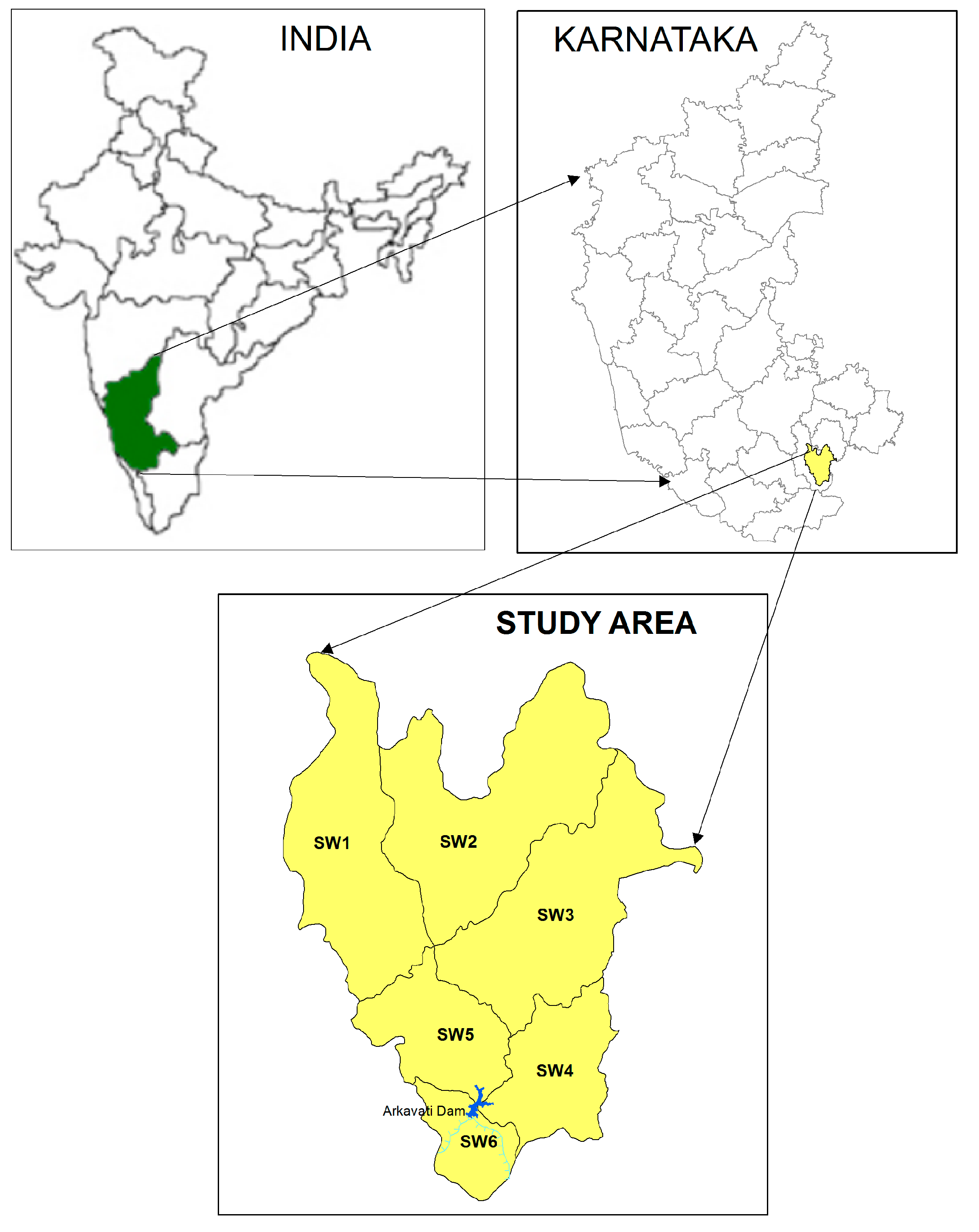
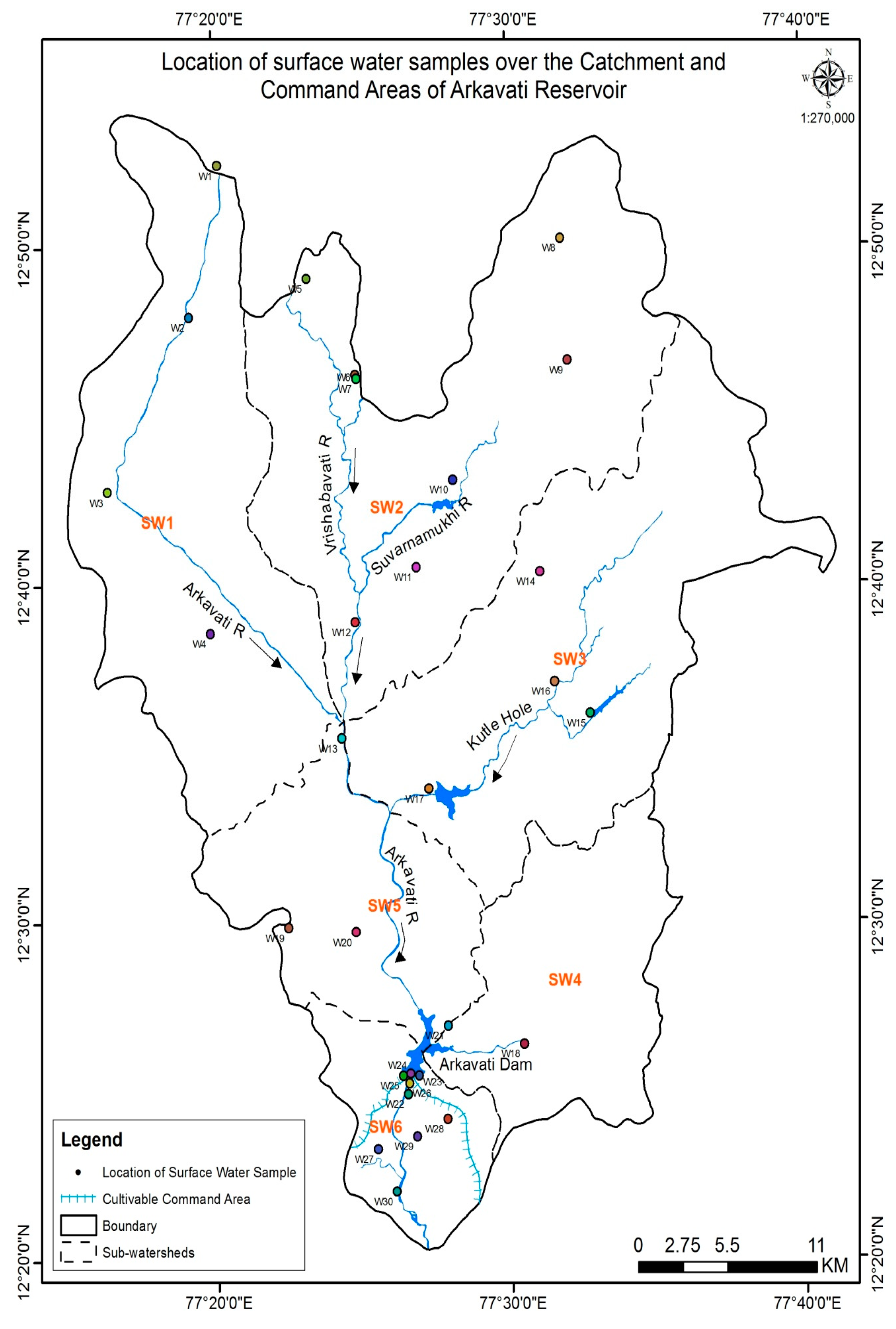
2.1. Study Area

The Arkavathi River, with a total flow length of about 210 kms, originates in the Nandidurga Hills (13°22′11″ N and 77°41′5″ E) of Karnataka state at an altitude of 1467 m amsl (above mean sea level) and flows through various parts of the region before draining into the Cauvery River, which is one of the most prominent rivers in southern India. The study area covered approximately 1572 km2 with a total perimeter 245.72 kms and is located between 12°20′ to 12°54′ N and 77°15′ to 77°44′ E (Figure 1, Figure 2, Figure 3, Figure 4 and Figure 5). The flow system of the main Arkavathi River from the point of its entry into the study area at Manchanabele Reservoir (12°52′19″ N and 77°20′5″ E) till its exit with a waterfall at Chunchi village (12°21′5″ N and 77°26′ 46″ E) is geologically structurally controlled. The Arkavathi River has a flow length of 65 kms from Manchanabele (720 m amsl) up to the Chunchi waterfalls (540 m amsl) and has a total fall in gradient of 180 m, i.e., an average fall in gradient of 2.8 m per km of flow length. The flow path of the subsidiary drainages is also linear. A total area of 62.32 km2 (cultivable command area), which is part of sub-watershed SW6, is irrigated with Arkavathi Reservoir water. The study area is demarcated into six sub-watersheds, which are named accordingly (Table 1) based on the drainage features of the area. The geology map of the study area is given in Figure 2. Contour maps, a digital elevation model map (prepared using RS and GIS), a slope map and a drainage map are given as online Supplementary Materials.

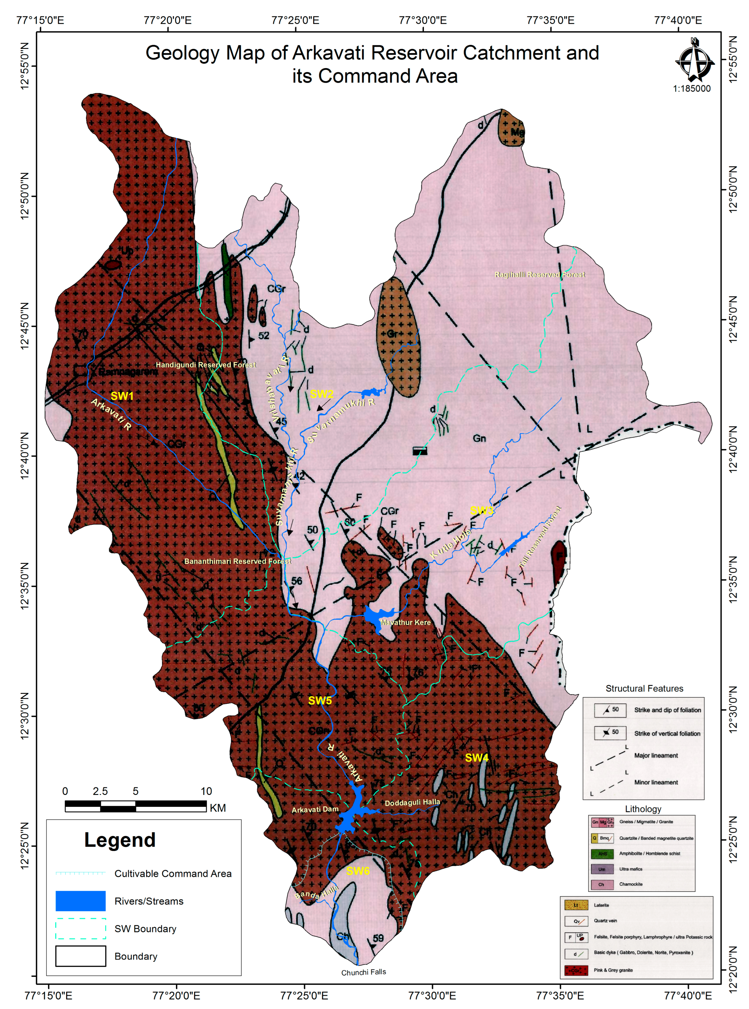
2.2. Geology and Geomorphological Features

A large extent of the Arkavathi Reservoir catchment and part of its command area, particularly the western parts, with a geomorphic display of abundant hills, hill ranges, inselbergs, intermittent valleys, rock-cut valleys, etc., is a type of area generally referred to as ‘Closepet Granites’. The Geology map of the study area (Figure 2) and a soil erosion map (Figure 3) are given here for reference. The hills at the eastern peripheral parts of the area are the southern extension of the granite belt [26]. This long but narrow intrusive rock body is composed of diorites, granodiorites and grey granites, and forms a divide between the Ponnaiyar River catchment to the east and the Vrishabhavati stream system of the Arkavathi sub-basin to the west. Suvarnamukhi, a subsidiary drainage of the Vrishabhavati stream, is born in the western part of this granite belt. The gneissic rocks of the younger gneissic complex are drained mainly by the Vrishabhavati stream system in the northcentral part of the area, which is bound by the Closepet Granites. The western part of the area, parallel to the southern-flowing Vrishabhavati stream, forms a longitudinal contact between the massive Closepet Granite body to the west and the young Gneissic group of rocks to the east. The Closepet Granites are of both grey and pink varieties and are coarse-grained and porphyritic. Granites are poorly jointed and are weathered to an average depth of 15 m in the valley zone. The depth of weathering thins out as we move towards the pediment part of the terrain.
Granite to the west and southern extension of the granite belt forms a moderately undulating topography. A small extent of the Arkavathi Reservoir command area also forms part of the gneissic terrain. Most of the gneissic terrain forms a pediplain with considerably weathered rock. The depth of weathering ranges up to 30 m. The gneissic rocks are easterly dipping, and the dip angle of the mineral foliation ranges from between 65° and 80°. Dip joints are more prominent. These gneissic rocks are fractured at the contact with granites, and the presence of pegmatites and quartz veins in gneisses are common.
A large part, excluding the part constituting hills and the hill range, forms the pediment zone. The presence of pediplains becomes transitionally significant from third-order streams and onwards. The thickness of soil is dependent upon the type of landscape. Red gravelly to loamy soils 0.3 to 1.5 m thick are commonly seen in the pediment part of the terrain, whereas the thickness ranges up to 2.5 m in the pediplain. While the hill range in the granite belt to the east of the southerly flowing Arkavathi River is N–S oriented, the hills west of the river (i.e., right bank catchment part) are E–W to ESE–WSW oriented. The height of the hills in the granite terrain ranges between 680 and 1043 m above mean sea level (amsl). These hills are massive and steep, and many are monoliths, with most of them attaining a height of more than 950 m amsl. The entire study area is a highly tectonically disturbed zone. South of 13° latitude, the Closepet Granite is flanked on its east by a ‘broad gravity low’ with its center near the town of Kanakapura (latitude 12°32′36″ N and longitude 77°25′2″ E).

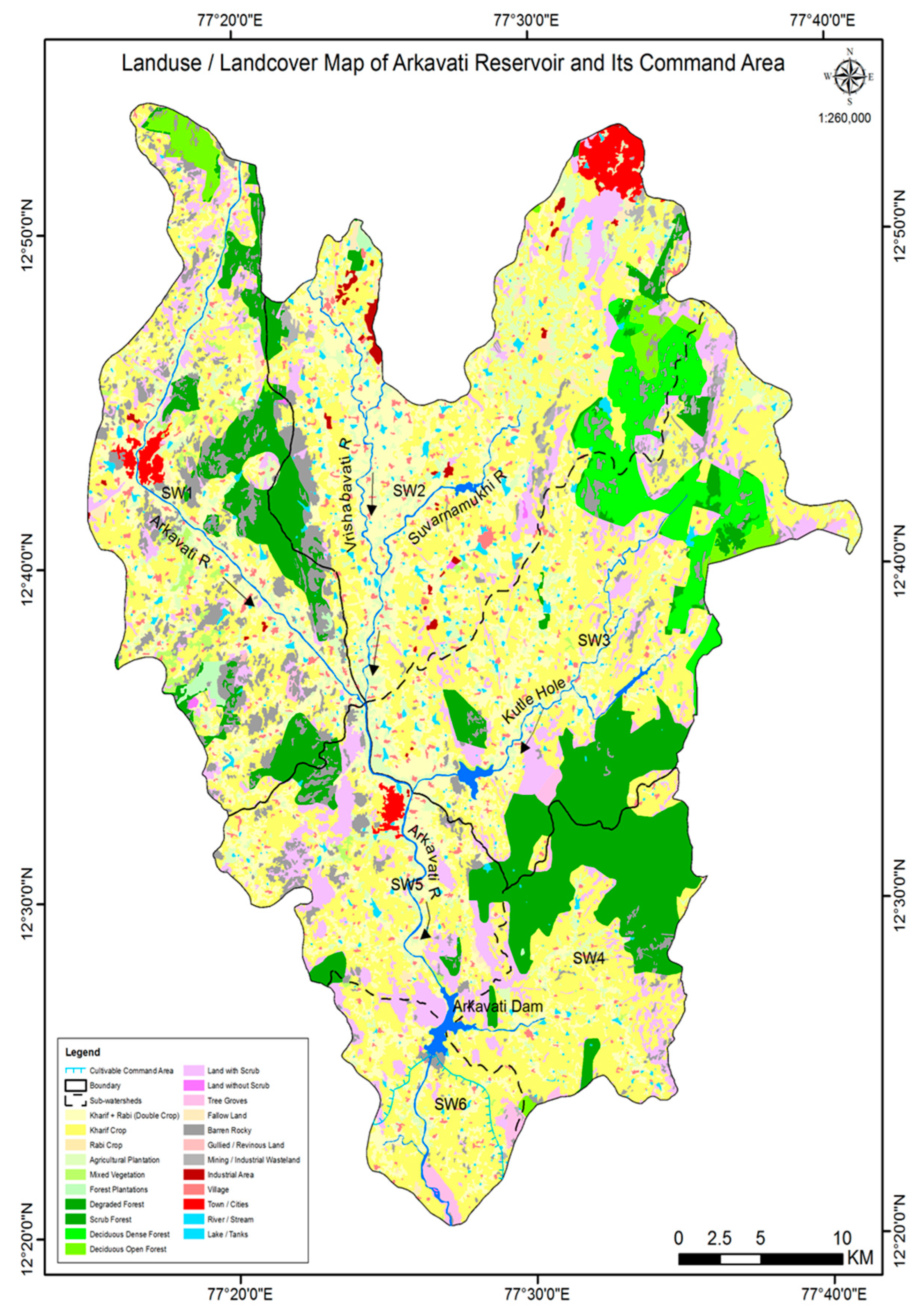
2.3. Land Use and Landcover of the Study Area

The study area is mainly composed of fertile land where kharif and rabi crops are grown (Figure 4). It also comprises scrub forest, land with scrub, agricultural plantations and an equal area of barren rocky sheetrock. A small portion of the area is occupied by moist, dry deciduous, dense and open forest. Though not significant, mining/industrial wasteland forms a minor part of the study area. Vegetation forms a major portion of the study area, along with a few villages and small towns. Sub-watershed areas SW1 and SW2 have townships along the Arkavathi River, where some cultivation takes places using the river water. This is true to some extent in SW5 as well. Human activity is increased in these three areas. SW3 and SW4 are predominantly forest and hilly areas with less human activity. However, SW4 has a significant number of quarries. SW6 is the command area and is rich in nutrients since it is mostly agricultural/irrigation land. A total area of 62.32 km2 (cultivable command area), which is part of sub-watershed (SW6), is irrigated with Arkavathi Reservoir water. Further details regarding land use and landcover are given in Table 2 below.

2.4. Sample Collection and Testing

Water samples were collected from 30 monitoring points over a study period of two years covering three prominent seasons of Pre-Monsoon, Monsoon and Post-Monsoon (Figure 5). To analyze the surface water quality of the area, we identified the sub-watersheds using Survey of India (SOI) Topographic Maps at 1:50,000 scale—57 H5, 57 H6, 57 H7, 57 H9, 57 H10 and 57 H11. Surface water samples within these sub-watersheds were then collected for further analysis. Two-liter polyethylene bottles/cans were thoroughly cleaned and were used to collect samples from the sampling locations. To avoid impurities on the surface of streams, the samples were drawn away from turbulence due to the banks and few centimeters below the water surface. For microbiological analysis of water samples, glass containers were used that could withstood 160 °C sterilization and would not produce or release any harmful chemicals that would inhibit biological activity, induce mortality or encourage growth. Samples for bacteriological examination were collected in clean, sterilized, narrow-mouthed, neutral glass bottles of 250 mL, 500 mL or 1000 mL capacity. The bottles were sterilized in a hot air oven at 100 °C for one hour. The sampling bottles were not opened except at the time of sampling. The detailed sampling (BIS, Part 1: Sampling [25]) and testing procedures for each of the contaminants along with the full dataset are given in the online Supplementary Materials section.
The samples were subjected to various physical, chemical and bacteriological tests as per the procedure given in [25] (Bureau of Indian Standards: Public Safety Standards of the Republic of India: Chemical: Environmental Protection and Waste Management: Part 1 to 63), as explained briefly in the Supplementary Materials. For example, to test for dissolved oxygen (DO), sampling and sample preservation were done as prescribed in BIS [25], Part 38: Dissolved Oxygen. The min–max ranges of the concentration levels of these parameters are provided in Table 3 for both years of the study.

2.5. Data Suitability

The KMO (Kaiser–Meyer–Olkin) (Kaiser, 1974) measure of sampling adequacy tests how well-suited the data are to perform FA. It measures the proportion of variance among parameters that might be common variances. KMO [27] returns a value between 0 and 1. If the value is closer to 1, it means that the data are better qualified for FA. In most of our analyses, we got a KMO value in the range of 0.6–0.7. Bartlett’s test of sphericity compares the correlation matrix to an identity matrix, i.e., it checks for redundancy between parameters. In this case, Bartlett’s test was very highly significant (<0.001), and, therefore, FA was appropriate. FA, clustering, ANOVA and t-tests were performed using the IBM SPSS statistical software [28] and XLSTAT Excel add-on data analysis package [29].

2.6. Multivariate Analysis

2.6.1. Factor Analysis

Principal factor analysis (PFA) is a dimension-reduction technique and was used as an extraction method [30,31,32] to reduce the large number of parameters while retaining most of the information contained in the original dataset. Factor analysis (FA) is a model-based statistical technique to bring out relationships between measured parameters and latent factors, which are unobserved parameters that are believed to be the cause of the measured values of observed parameters. The assumption is that correlations between observed parameters are due to the causal influence of one or more factors (latent parameters). Each principal component is identified with its eigenvalue and eigenvector. The eigenvalue for each component (or factor, in the case of FA) measures the variance in all the parameters that are accounted for by that component. Factors can be better interpreted with rotation, a process which increases the loading of different parameters on the extracted factors while reducing their loading on the rejected factors. There are different methods of rotation, which can mainly be divided into two categories. Orthogonal rotations such as varimax are useful if factors are expected to be unrelated, while oblique rotations such as oblimin are more applicable if some correlation between the extracted factors is expected. Further details on the outcome of FA are given in the results (Section 3.1 below).

2.6.2. Cluster Analysis

Cluster analysis has been used with good success in various studies of water quality around the world. It is usually used in conjunction with other multivariate analyses as a spatial clustering tool [33] or for assessing seasonal and spatial variability of water quality [34]. In this study, the distance between datapoints was calculated by the Euclidean distance in m-dimensional space, and agglomerative hierarchical clustering (AHC) was used for clustering. An agglomeration criterion such as unweighted pair–group average was used to minimize and form clusters. Here, we clustered the dataset based on observations, i.e., the points at which samples were collected; this was done across all the parameters.

2.6.3. Two-Way and Three-Way ANOVA and t-Tests

Analysis of variance (ANOVA) is a statistical tool that tests the hypothesis of whether there are any differences in the means of a group of datasets or not [35,36]. The null hypothesis in ANOVA is that the means of subjects are the same in different groups, and the alternative hypothesis is that there is a statistically significant difference in the means—either between one group compared to all others or between multiple groups within the study. On the other hand, for comparing whether the means of only two groups are related or not, the t-test is used. Since sampling was conducted across three seasons over two years, a total of six datasets for each parameter were expected for analysis. Attention was drawn to some of the prominent parameters discovered in FA to avoid repetition of analysis of similar parameters or similar groups of parameters. The repeated measures considered in two-way ANOVA were the two factors of “season” and “year” together, while three-way ANOVA was used to consider the additional aspect of “sampling location”. The repeated measures method was used because the data from the same set of samples were used but across different seasons and different years.

3. Results and Discussion

3.1. Factor Groupings
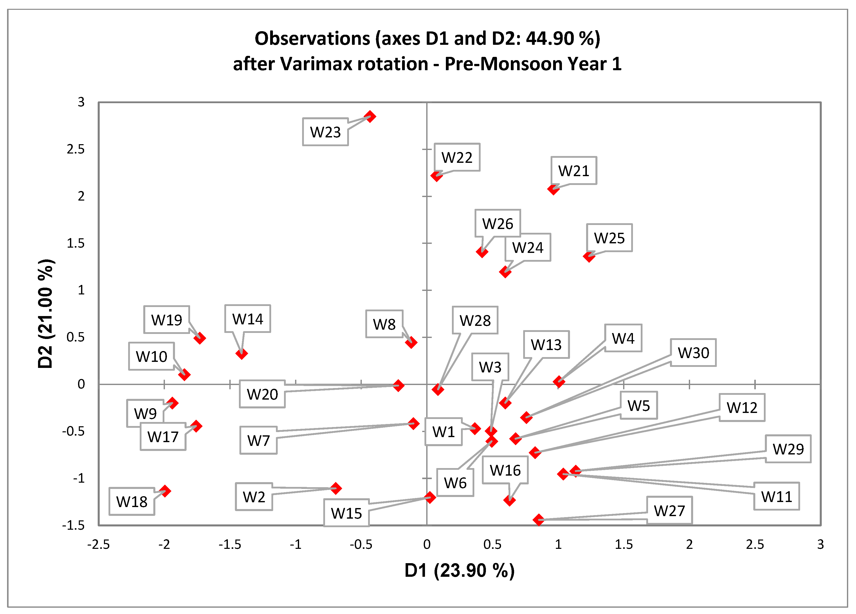
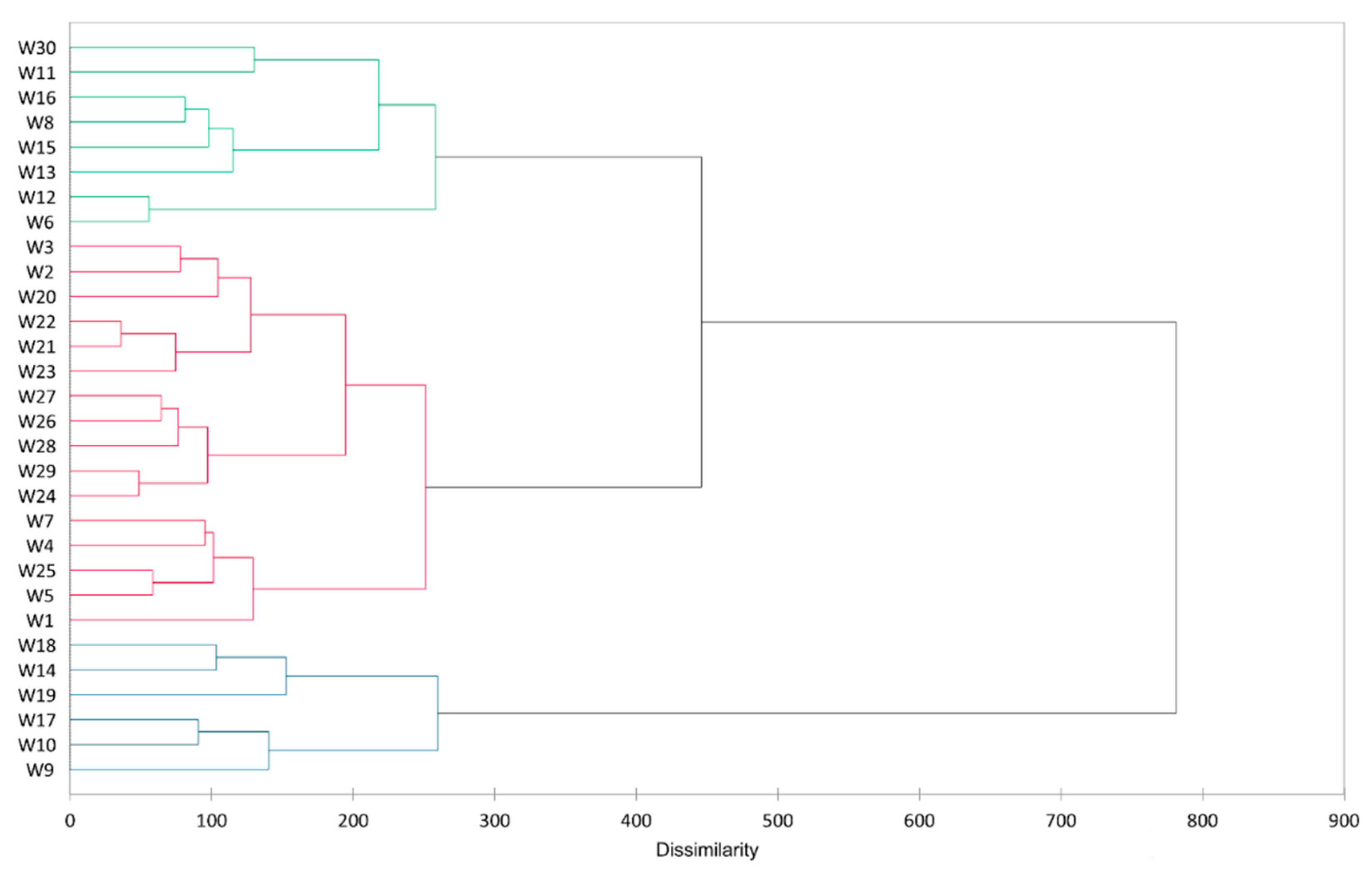
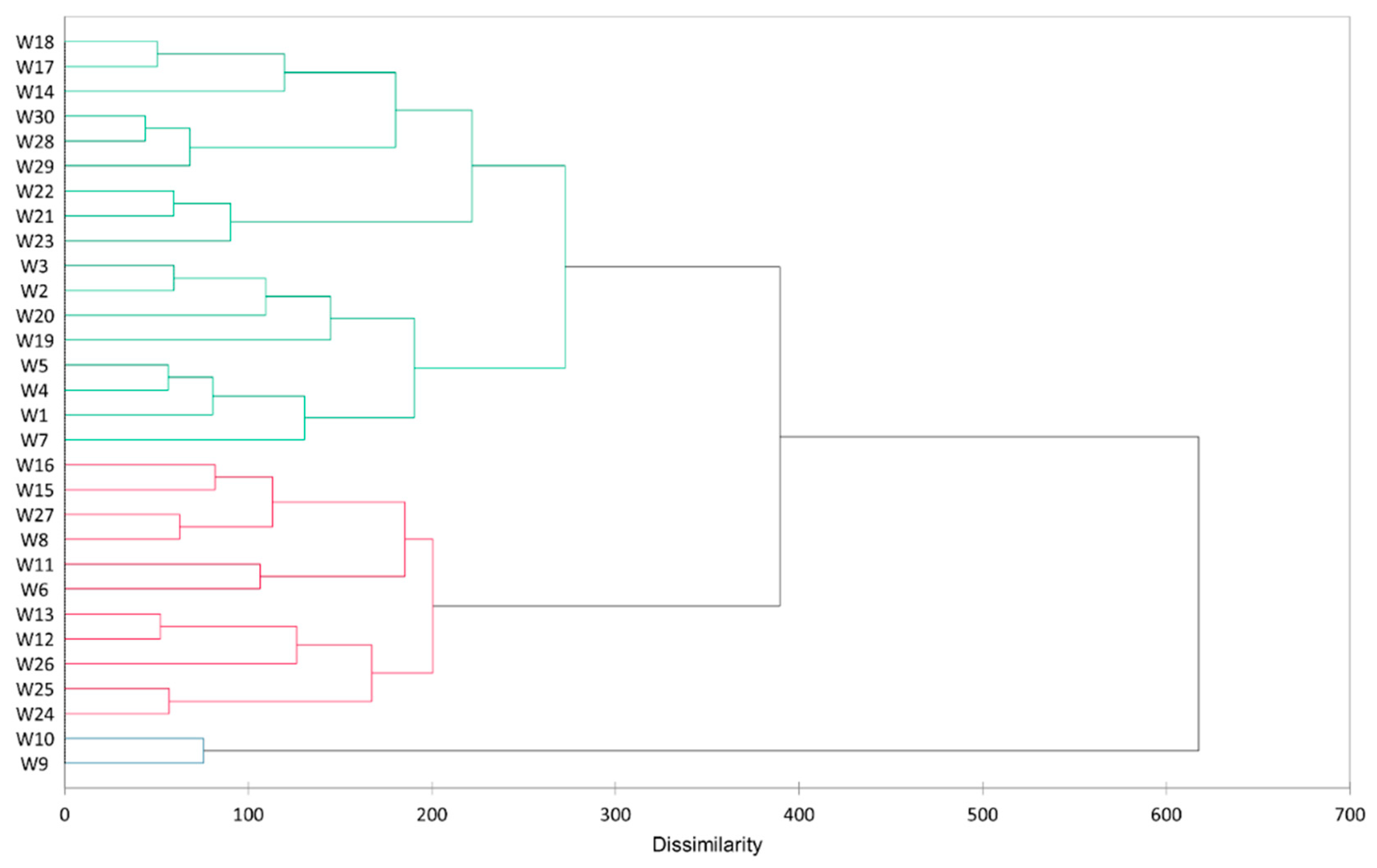
The total variance explained for the dataset of the Pre-Monsoon season of the first year in terms of variability (%) per factor is 41.70, 13.50, 9.76, 6.39 and 3.25 for the first five factors, whose eigenvalues were >1. The cumulative variance for these first 5 factors is 74.6%, and for the first 12 factors it is 82.34%, as shown in the scree plot in Figure 6. We used varimax rotation to increase the loading of different parameters on the extracted factors. We then found that five new rotated factors (D1 through D5) accounted for a cumulative variation of approximately 75%, as shown in Table 4.
Table 5 gives the component matrix or factor loadings for each of the five rotated factors for the Pre-Monsoon season. The corresponding matrices for the monsoon and Post-Monsoon seasons for Year 1 are given in Table A1 in Appendix A. The values in bold in Table 5, when read down through each column, indicate the groupings of the parameters that influenced the corresponding factor to a similar extent. During the Pre-Monsoon season, Factor 1 (D1) was influenced by parameter groupings TDS–EC, Cations K+, Ca2+, Mg2+, Total Hardness, Cl , HCO 3 and Total Alkalinity. These parameters loaded strongly on D1 and hence are related to each other and can be grouped together. This grouping was largely carried forward during the monsoon season, but during the Post-Monsoon period, TDS and EC formed a separate grouping on D4, while Na+, K+, Ca2+, Mg2+, Cl and HCO 3 formed a distinct group based on their loading on D2. For both years, TDS and EC consistently loaded together on the same factor across all seasons. The more salts dissolved in the water, the higher the value of EC. Hence, TDS and EC grouped together. Similar is the case with BOD5–COD and Total Coliform–Fecal Coliform and the group of Cations (Na+, K+, Ca2+, Mg2+), Total Hardness, HCO 3 and Total Alkalinity. The granitic material of the study area contains mineral feldspar, which is composed of sodium, potassium and calcium, hence the grouping of these ions.
BOD5 (for 5 days) and COD were consistently grouped together across all the seasons. This is because BOD is the oxygen demand of organic matter in water, whereas COD is the oxygen demand of organic and inorganic matter. We also noticed that pH and DO loaded negatively with BOD5 and COD during Pre-Monsoon, and this negative linkage incrementally changed from the Pre- to Post-Monsoon seasons. High COD concentrations indicate organic and inorganic pollution [37]. Increased nutrient concentration leads to increased organic matter concentration, and the consequent respiration and degradation of organic matter reduces DO concentration [38]. There was another interesting grouping of BOD5 and COD with Total and Fecal Coliforms in Pre-Monsoon, which reduced significantly during the Monsoon season and again became slightly more positively linked during the Post-Monsoon season. This was due to the population density of Fecal Coliform in the river being directly proportional to the degree of sewage pollution, which was reflected by BOD5 levels [39]. Though heavy metals were largely nonexistent due to a smaller number of industrial sites, Fe2+ and Zn2+ formed a group and loaded together during the Monsoon and Post-Monsoon seasons. Turbidity and Fe2+ loaded together on the same factor consistently across seasons since iron content in the form of colloidal particles contributes to turbidity [40]. FA not only allows us to track the evolution of these groupings/relationships through the season, but, as shown in Figure 7, it also validates the clustering of datapoints based on the sampling locations across the study area. It confirms the clusters formulated through AHC (Section 3.2, Figure 8) by plotting the observation points onto the rotated factor axes D1, D2 as shown in Figure 7.

3.2. Clustering

While samples from sub-watersheds SW1 and SW6 formed clear clusters, the clustering is varied in other sub-watersheds. Sampling locations W9, W10, W14, W17, W18 and W19 formed a distinct cluster during Pre-Monsoon and Monsoon seasons since these sampling points are located in hilly areas in sub-watersheds SW3, SW4, SW5 and partially in SW2. Dendrogram representations revealed, as shown in Figure 8 for Pre-Monsoon season of Year 1 and Figure A1 and Figure A2 in Appendix A for the Monsoon and Post-Monsoon seasons, respectively, that the locations W1, W2, W3, W4, W5, W7 and W20 formed a subcluster not only during the Pre-Monsoon season of Year 1, but also during the Post-Monsoon season due to these samples being upstream from the reservoir and around the main Arkavathi River. W21, W22 and W23 formed smaller subclusters over all the seasons. W26, W27, W28, W29 and W30 formed a subcluster due to their location in the command area downstream from the reservoir (sub-watershed SW6), with irrigation activities being similar in these locations. Another interesting subcluster formation was of W6, W11 and, W12 and W8, W13, W15 and W16 (due to these locations being covered with scrub) across all three seasons. This is confirmed further by the distance to the cluster centroids, where points W6, W11 and W12 have similar distances to the centroids, while W8, W13, W15 and W16 have different distances to the same cluster centroid. For Year 2 observations, the clusters largely remain the same. For example, W9, W10, W14, W17, W18 and W19 form a distinct cluster during the Pre-Monsoon and Monsoon seasons. However, W9 and W10 form a separate cluster during the Post-Monsoon season. The other subclusters also largely follow patterns similar to those of Year 1.

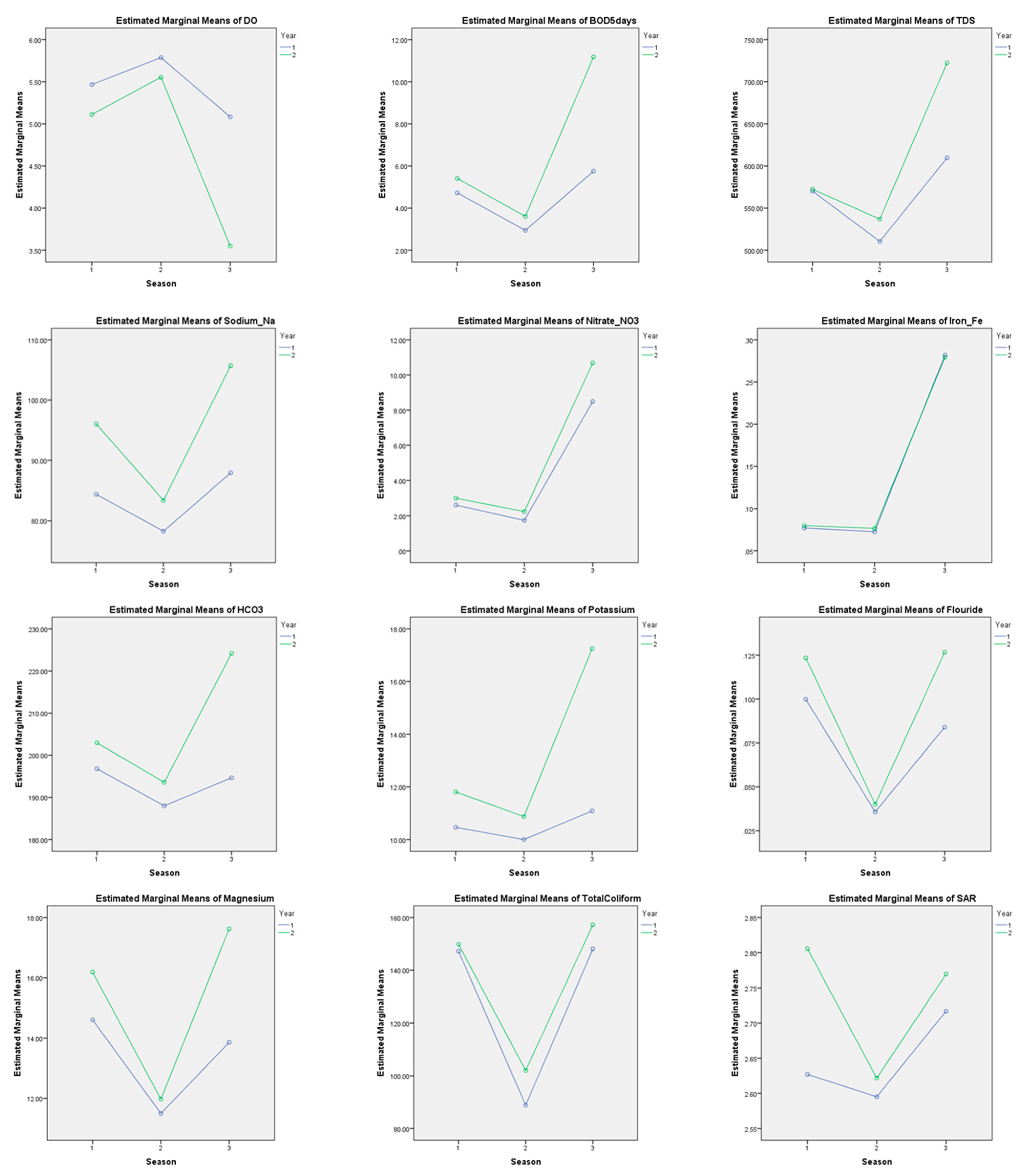
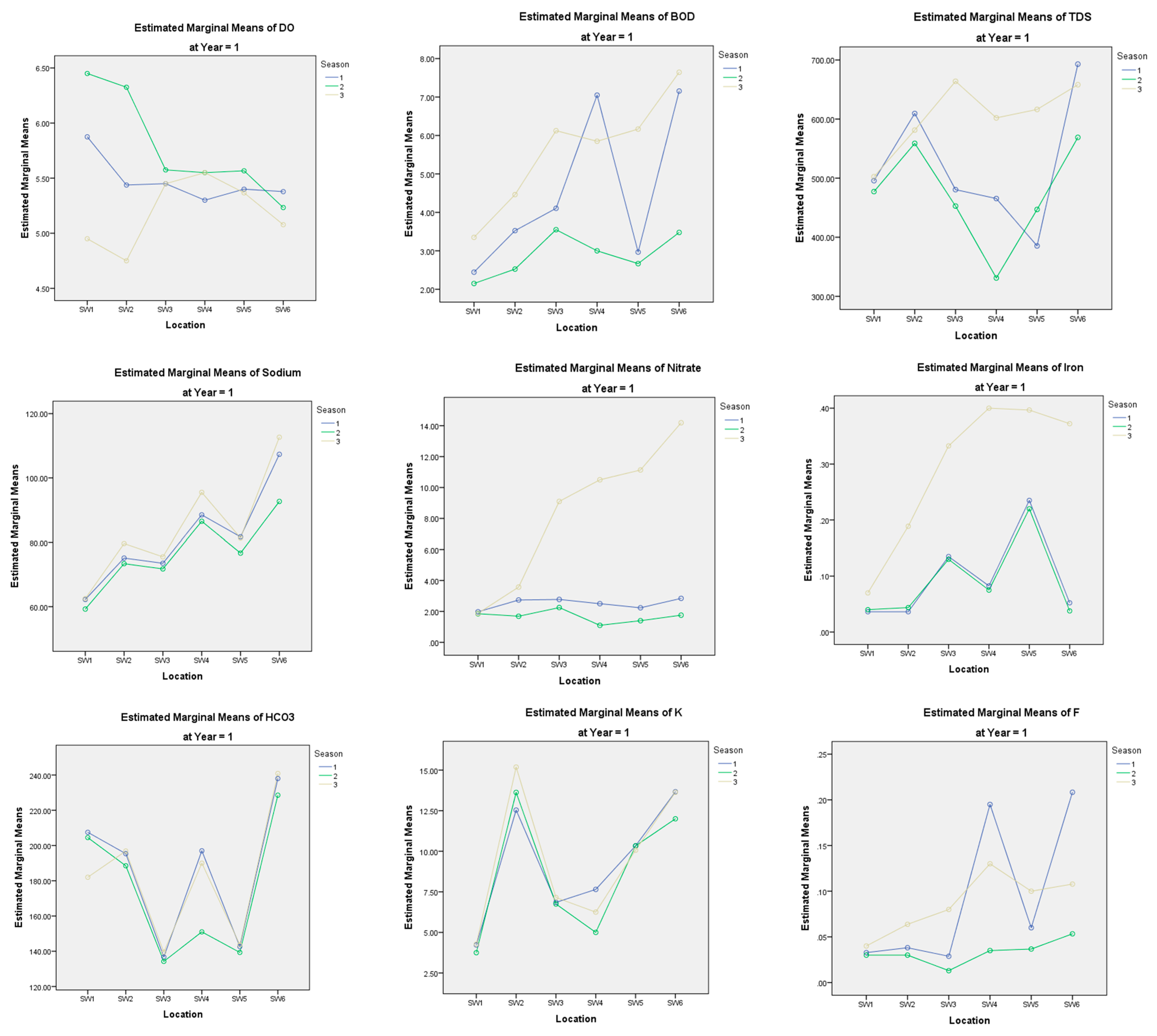
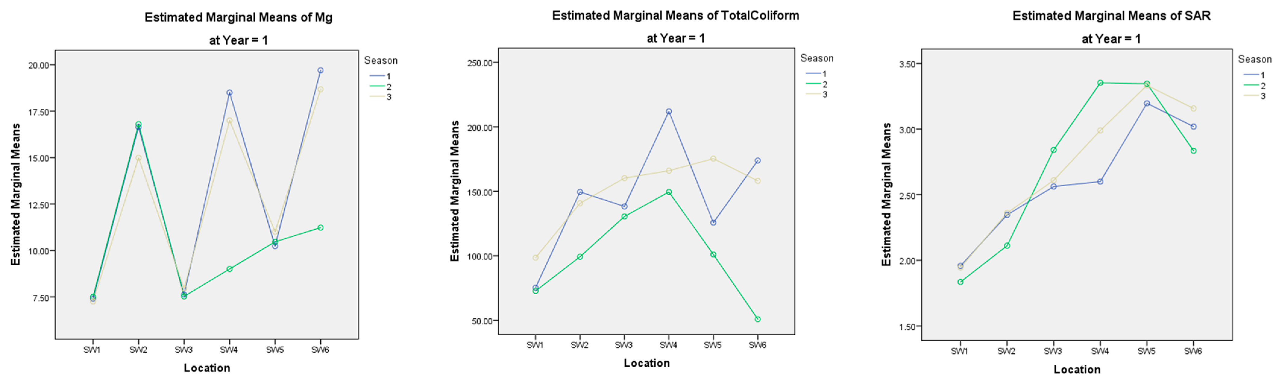
3.3. Two-Way and Three-Way ANOVA: Effects due to Years, Seasons and Locations

For comparing differences between years, two-way ANOVA [35,36] was applied to compare the means between seasons and across the two years, as shown in Figure 9 below. The mean concentration levels across seasons and years and the corresponding F-statistics are given in Table A2 in Appendix A. For DO, the F-statistic was F(1,29) = 69.16 for the variation between years (considered over all seasons), which was very highly significant at p < 0.001, while the seasonal variation (considered across both years) had F(2,58) = 56.51, which was also very highly significant with p < 0.001. This showed that when the effects of both seasonal and yearly variation were considered, the DO levels were significantly different across seasons and years. Similarly, the mean BOD5 levels were different across seasons (5.069 mg/L, 3.275 mg/L and 8.467 mg/L) with F(1,29) = 139.997 and p < 0.001 and across the two years (4.474 mg/L and 6.733 mg/L) with F(2,58) = 55.608 and p < 0.001. Similarly, mean levels of other parameters such as TDS, TSS, NO 3 , Na+ and Total Hardness were statistically different across seasons and years. We found that most of the physical and chemical parameters were diluted and displayed lower concentrations during the Monsoon season versus during Pre- or Post-Monsoon seasons. Additionally, in cases such as that of Mg2+ and F , results showed that, while Monsoon levels were substantially different to that of Pre- and Post-Monsoon levels, there was no difference in concentration levels of F between Pre- and Post-Monsoon levels in the case of both years. The mean Total Coliform levels were different across seasons (148.517 MPN/100 mL, 95.45 MPN/100 mL and 152.65 MPN/100 mL) with F(2,58) = 21.97 and p = 0.01, and across the two years (128.04 MPN/100 mL and 136.37 MPN/100 mL) with F(1,29) = 38.44 and p < 0.001; also, the effect of interaction between seasons and years was strong with regard to the mean levels of Total Coliform, with F(2,58) = 4.25 and p = 0.019. In the case of Total Coliform levels, however, paired t-tests between pairs of seasons for both years showed that, while Monsoon levels were substantially different from those of Pre- and Post-Monsoon levels, there were no difference in concentration levels of Total Coliform between Pre- and Post-Monsoon season in the case of both years.
On applying three-way ANOVA (to consider the effect of sampling locations), we observed that there were some differences in mean levels of most of the parameters across different sub-watersheds. BOD5, Na+, NO 3 , Fe2+, HCO 3 , K+, F , SAR and COD all showed significant (p < 0.05) differences between concentration levels across the six sub-watershed locations (Figure 10, Table A3 in Appendix A). Further, the parameters BOD5, Total Hardness, NO 3 , K+, Ca2+, F, SAR and COD showed statistically strong differences in mean values when interactions between year, location and seasons were considered together. Since organic-pollution-loading in water bodies increases from upstream to downstream from the reservoir, BOD5 and COD of water samples increased, while DO decreased as we moved along from SW1 to SW6 due to addition of sewage and other domestic activities along the river course. Since nitrate is the representation of oxidized organic matter in water and is one of the main components of fertilizers used in irrigation, and its presence increases BOD5, nitrates varied similar to BOD5 with respect to location, especially during the Post-Monsoon season. Due to run-off, TDS was especially high in SW6, indicating potential soil erosion in upper sub-watersheds. This is supported by the soil erosion map (see online Supplementary Materials), which indicates high soil erosion in SW3, SW4 and SW5. The presence of iron in natural waters can be attributed to the dissolution of rock and minerals containing biotite as part of the weathering process. We observed that iron content was higher in the forest and hilly areas SW3, SW4 and SW5. Similarly, Mg was high in SW4 and SW6.

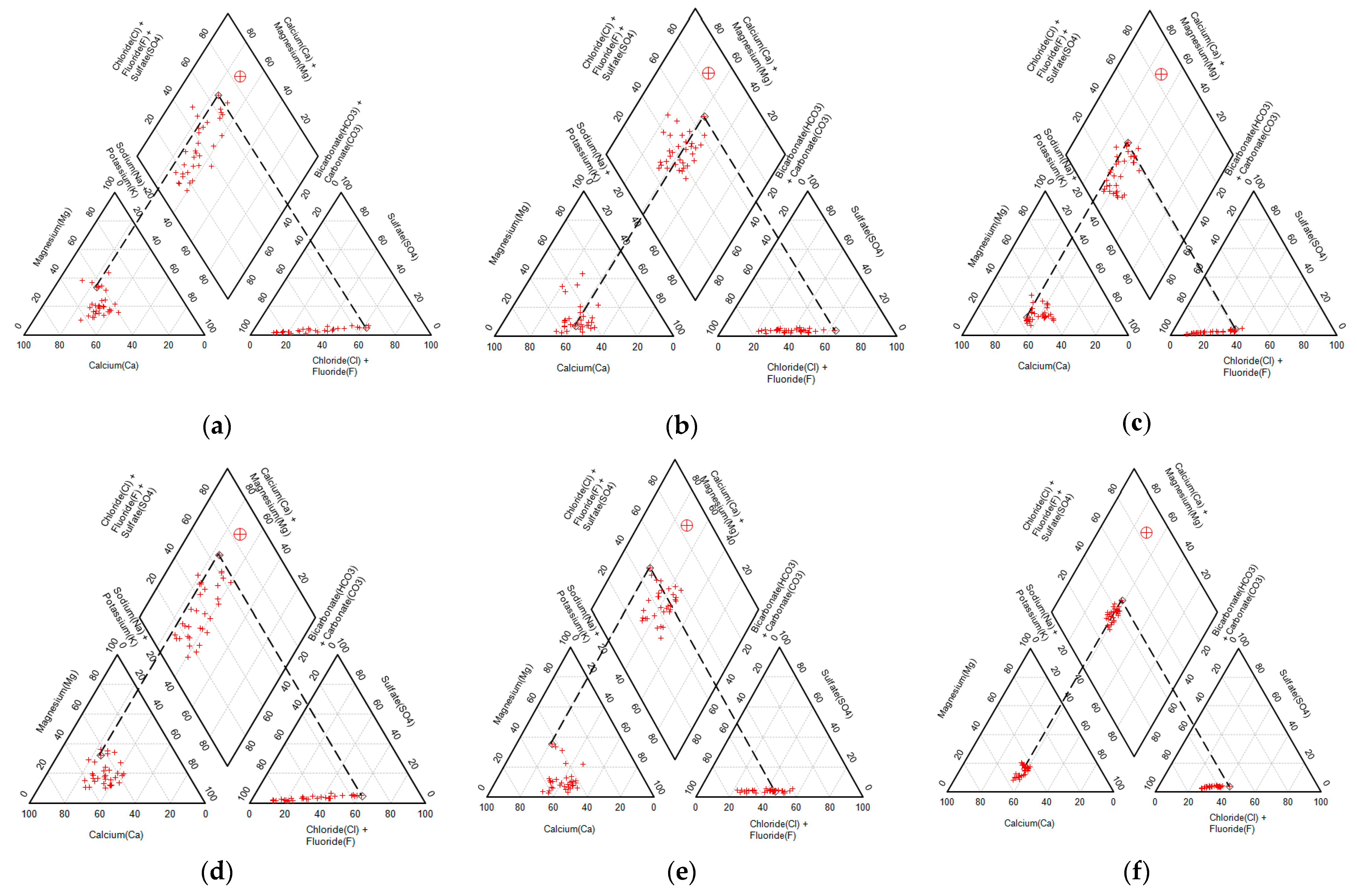
3.4. Groundwater Quality of the Study Area—Piper Trilinear Diagrams

The objective of groundwater analysis is to understand the groundwater chemistry, the impact of land use and landcover changes on quality of groundwater, and to suggest suitable measures to improve groundwater quality. This is important as local populations depend on groundwater to supplement surface water. A total of 33 groundwater samples were collected for each of the three monsoon seasons over a period of two years. Based on the results of the analysis, Piper Trilinear diagrams were generated to interpret the groundwater chemistry and the conclusions were noted. Graphical interpretation of groundwater quality of the study area is necessary since it contains minerals that are to be assessed for the irrigation suitability. A Piper Trilinear diagram is useful for bringing out the chemical relationships between groundwater samples in more definite terms than available with other plotting methods [41]. This plot helps in understanding and identifying the water composition in different classes. The triangular plots of major anions and major cations have been successfully used in the interpretation of results of groundwater from aquifers of the Calabria region (southern Italy) [23]. Piper Trilinear diagrams generated for groundwater for the three seasons and over the two years of study are presented in Figure 11a–f. They reveal the analogies, dissimilarities and different types of water in the study area as identified and listed in Table 6. It can be concluded from the below results that during the Pre-Monsoon and Monsoon seasons, most of the samples consist of calcium and magnesium bicarbonate waters, which is typically shallow, fresh groundwater, and a few samples are of calcium and magnesium sulfate waters, which is typically gypsum groundwater. During the Post-Monsoon season of both the years, all samples are of calcium and magnesium bicarbonate waters, which is typically shallow, fresh groundwater. This indicates that Ca and Mg are dominant in the groundwater of the study area during the study period.

4. Conclusions

In this study, we carried out a comprehensive multivariate statistical analysis of the concentration levels of physical, chemical and biological parameters in surface water samples collected from six sub-watersheds of the Arkavathi Reservoir catchment and command area over a period of two years (2013 and 2014) and three seasons of monsoon (Pre-Monsoon, Monsoon and Post-Monsoon). We also conducted chemical analysis of groundwater of the study area and classified the groundwater based on Piper Trilinear diagrams. The present study demonstrates the applicability of FA–AHC–ANOVA as a significant analysis tool for effective watershed management to improve water quality in rivers and reservoir catchment and command areas. This work forms a basis for further exploration of variations of such surface water contaminants in different terrains and watersheds worldwide. A few specific, significant recommendations follow:
  • Considering the many townships along the Arkavathi River in SW1, domestic sewage needs to be treated effectively at the border region of SW1 and SW5 and within SW6, especially during the Post-Monsoon season.
  • Usage of fertilizers, especially in the agricultural lands in command area SW6, should be closely monitored and controlled.
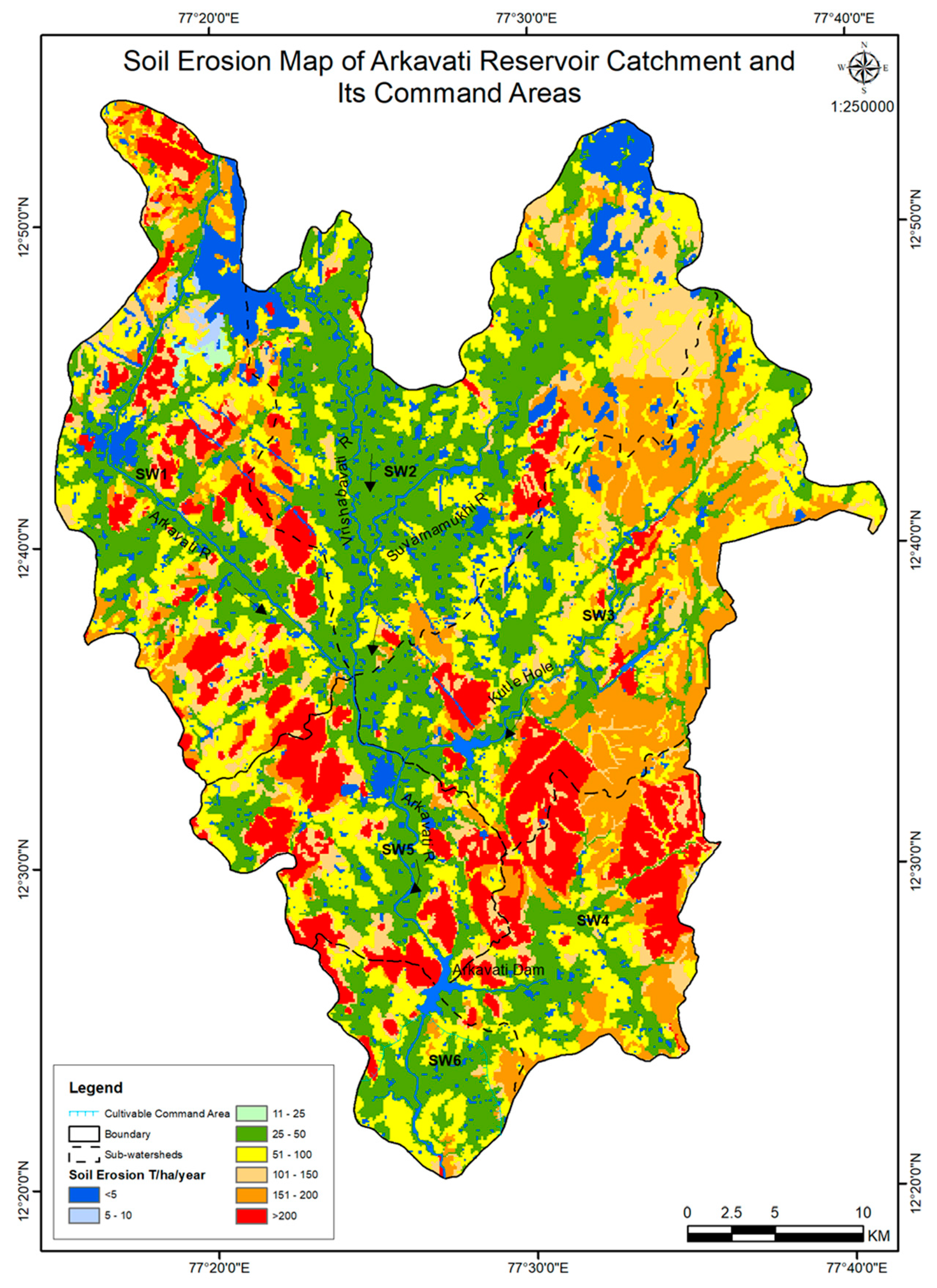
  • Erosion control plans need to be put in place in SW3, SW4 and SW5, as indicated by high TDS in SW6.
  • Quarry activities in SW4 and SW3 need to be monitored for potential contamination of smaller streams.

Supplementary Materials

The following supporting information can be downloaded at: http://doi.org/10.17632/rwcw59p9g2.7: Contour map; Digital Elevation Model map; Drainage map; Slope map; Full Dataset; and Sampling and testing procedure.

Author Contributions

Conceptualization, J.R.S.K.; methodology, J.R.S.K. and V.H.P.; software, V.H.P.; validation, J.R.S.K.; formal analysis, J.R.S.K. and V.H.P.; investigation, J.R.S.K.; resources, J.R.S.K.; data cura-tion, J.R.S.K.; writing—original draft preparation, J.R.S.K. and V.H.P.; writing—review and edit-ing, J.R.S.K. and V.H.P.; visualization, J.R.S.K. and V.H.P.; supervision, J.R.S.K.; project admin-istration, J.R.S.K. All authors have read and agreed to the published version of the manuscript.

Funding

This research received no external funding.

Data Availability Statement

The full dataset is available at http://doi.org/10.17632/rwcw59p9g2.7.

Acknowledgments

The authors are thankful to Chandrashekar. H, Senior Lecturer, MEI Polytechnic, Bengaluru, India for his guidance in locating and collecting the samples. The authors would also like to thank Subhash Chandra K C, Retired Senior Hydrogeologist, Mines and Geology Department, Karnataka State, India, for his guidance regarding the geological aspects of the study. The authors would also like to thank the anonymous reviewers whose helpful comments have aided in improving the final draft of this article.

Conflicts of Interest

The authors declare no conflict of interest.

Appendix A

Figure A1. Dendrogram of sampling/observation points for the Monsoon season of Year 1.
Water 14 02359 g0a1
Figure A2. Dendrogram of sampling/observation points for the Post-Monsoon season of Year 1.
Water 14 02359 g0a2
Table A1. Factor pattern or the rotated component matrix for Monsoon and Post-Monsoon seasons of Year 1.
MonsoonPost-Monsoon
D1D2D3D4D5D1D2D3D4D5
pH−0.015−0.3790.225−0.031−0.134−0.011−0.212−0.030−0.089−0.509
DO0.008−0.523−0.4280.157−0.383−0.267−0.1030.747−0.0030.017
BOD50.1900.3250.2690.1640.7390.4770.073−0.0120.1690.811
COD0.0570.052−0.410−0.0030.6940.5090.063−0.0060.1820.783
TSS0.046−0.621−0.0440.0320.1050.6950.333−0.3790.1050.291
Turbidity−0.039−0.1170.9650.0840.1610.8600.258−0.0430.186−0.070
TDS0.889−0.0470.059−0.0760.2130.2720.2960.0290.8880.201
Conductivity0.895−0.0570.065−0.0800.2090.2740.2970.0220.8880.198
Na+0.5180.726−0.001−0.1420.2830.4360.7440.2970.1250.307
K+0.6400.164−0.219−0.054−0.080−0.0880.523−0.1440.4110.349
Ca2+0.863−0.186−0.003−0.1990.2050.1070.699−0.2690.126−0.217
Mg2+0.6970.158−0.1620.264−0.3310.2420.7690.0280.1760.144
Total hardness as CaCO30.935−0.067−0.0060.011−0.0850.7620.386−0.0740.2870.219
Cl 0.7960.446−0.0930.0760.2370.3220.8490.0420.0920.055
HCO 3 0.7750.239−0.270−0.3950.0510.0350.896−0.0450.1900.166
F 0.2030.479−0.249−0.4130.3180.7650.279−0.1500.0820.243
NO 3 0.523−0.3470.1350.0390.2860.6010.1560.1500.1580.673
[ PO 4 ] 3 −0.275−0.3620.3500.1740.0220.7150.0270.0530.0110.325
SO 4 2 0.668−0.3640.0710.045−0.3080.7600.443−0.045−0.0310.109
Fe2+−0.1720.0260.7930.090−0.0890.690−0.1540.1860.0960.618
Zn2+0.1200.0970.5510.340−0.1570.7940.277−0.3290.1090.310
Total alkalinity as CaCO30.7340.082−0.234−0.4300.0350.7690.3400.0230.3210.095
Total coliform/100 mL−0.113−0.1800.1720.872−0.0140.742−0.1330.0330.1720.378
Fecal coliform/100 mL−0.0940.0390.0820.9520.1440.713−0.0620.2680.1850.575
SAR−0.2820.7750.1100.0050.1030.3520.1680.5440.0580.399
Note: Values in bold for each parameter correspond to the factor for which the squared cosine is the largest [30].
Table A2. Mean concentration levels of a few parameters across seasons and years, and the corresponding F-statistic.
Pre-MonsoonMonsoonPost-MonsoonF-Statistic for SeasonsYear 1Year 2F-Statistic for YearsF-Statistic for Interaction between Seasons and Years
ParameterMean concentration level (mg/L)Mean concentration level (mg/L)Mean concentration level (mg/L)(F(2,58) at p < 0.001)Mean concentration level (mg/L)Mean concentration level (mg/L)(F(1,29) at p < 0.001)(F(2,58) at p < 0.001)
TDS571.27523.72666.1514.58563.48610.6129.2220.59
TSS5.0654.2307.7236.0335.116.23101.7324.56
NO 3 2.8041.9879.5852.84.285.3179.2522.61
Na+90.2280.8296.8322.2283.5395.0437.378.676 (p = 0.001)
Total Hardness242.017201.688347.8347.04249.29278.453.0231.02
Mg2+15.39711.7415.749.2 (p = 0.01)13.3215.2627.017.437
F 0.1120.0380.10512.21 (p = 0.01)0.0730.09722.613.97
Ca2+61.7362.0369.684.93 (p = 0.01)59.0569.9176.7322.35
HCO 3 199.88190.78209.434.91 (p = 0.01)193.156206.9128.349.48
K+11.1410.4414.1724.55 (p = 0.01)10.5213.3147.1718.16
Table A3. Tests of between-subject effects of surface water when location is considered.
SourceMeasureType III Sum of SquaresdfMean SquareFSig.Partial Eta Squared
LocationDO13.50052.7001.3480.2790.219
BOD5465.845593.1697.2390.0000.601
TDS806,893.1565161,378.6311.1050.3840.187
TSS92.440518.4881.6800.1780.259
Na+54,851.996510,970.3996.2120.0010.564
Total Hardness229,868.853545,973.7711.4360.2470.230
NO 3 558.4405111.6889.6260.0000.667
Fe2+0.79650.1599.4610.0000.663
HCO 3 196,681.589539,336.3183.3280.0200.409
K+2739.1245547.8256.7480.0000.584
Ca2+17,471.29353494.2591.5810.2030.248
F 0.39750.0795.2600.0020.523
Mg2+2795.7725559.1542.0260.1110.297
Total Coliform95,860.353519,172.0712.1360.0960.308
SAR38.72457.7456.9470.0000.591
COD1677.7075335.5417.4830.0000.609
ErrorDO48.084242.003
BOD5308.9062412.871
TDS3,505,192.48824146,049.687
TSS264.0952411.004
Na+42,387.315241766.138
Total Hardness768231.2992432,009.637
NO 3 278.4712411.603
Fe2+0.404240.017
HCO 3 283,709.8772411,821.245
K+1948.3452481.181
Ca2+53,035.943242209.831
F 0.362240.015
Mg2+6623.99324276.000
Total Coliform215,430.875248976.286
SAR26.758241.115
COD1076.2172444.842

References

  1. Iticescu, C.; Georgescu, L.P.; Murariu, G.; Topa, C.; Timofti, M.; Pintilie, V.; Arseni, M. Lower Danube Water Quality Quantified through WQI and Multivariate Analysis. Water 2019, 11, 1305. [Google Scholar] [CrossRef] [Green Version]
  2. Wang, X.; Zhang, F. Multi-Scale Analysis of the Relationship between Landscape Patterns and a Water Quality Index (WQI) Based on a Stepwise Linear Regression (SLR) and Geographically Weighted Regression (GWR) in the Ebinur Lake Oasis. Environ. Sci. Pollut. Res. 2018, 25, 7033–7048. [Google Scholar] [CrossRef] [PubMed]
  3. Olsen, R.L.; Chappell, R.W.; Loftis, J.C. Water Quality Sample Collection, Data Treatment and Results Presentation for Principal Components Analysis—Literature Review and Illinois River Watershed Case Study. Water Res. 2012, 46, 3110–3122. [Google Scholar] [CrossRef] [PubMed]
  4. Cheng, G.; Wang, M.; Chen, Y.; Gao, W. Source Apportionment of Water Pollutants in the Upstream of Yangtze River Using APCS–MLR. Environ. Geochem. Health 2020, 42, 3795–3810. [Google Scholar] [CrossRef] [PubMed]
  5. Matamoros, V.; Arias, C.A.; Nguyen, L.X.; Salvadó, V.; Brix, H. Occurrence and Behavior of Emerging Contaminants in Surface Water and a Restored Wetland. Chemosphere 2012, 88, 1083–1089. [Google Scholar] [CrossRef]
  6. González, S.; López-Roldán, R.; Cortina, J.L. Presence and Biological Effects of Emerging Contaminants in Llobregat River Basin: A Review. Environ. Pollut. 2012, 161, 83–92. [Google Scholar] [CrossRef] [PubMed]
  7. Boyacioglu, H. Surface Water Quality Assessment Using Factor Analysis. Water SA 2006, 32, 43. [Google Scholar] [CrossRef] [Green Version]
  8. Dani, A.; Bărbulescu, A. Statistical Analysis of the Water Quality of the Major Rivers in India. In Frontiers in Water-Energy-Nexus—Nature-Based Solutions, Advanced Technologies and Best Practices for Environmental Sustainability, Proceedings of the 2nd WaterEnergyNEXUS Conference, Salerno, Italy, 14–17 November 2018; Naddeo, V., Balakrishnan, M., Choo, K.-H., Eds.; Springer: Cham, Switzerland, 2020; pp. 281–283. [Google Scholar]
  9. Hamil, S.; Bouchelouche, D.; Arab, S.; Doukhandji, N.; Smaoune, G.; Baha, M.; Arab, A. Statistical Multivariate Analysis Assessment of Dams’ Water Quality in the North-Central Algeria. In Advances in Sustainable and Environmental Hydrology, Hydrogeology, Hydrochemistry and Water Resources, Proceedings of the 1st Springer Conference of the Arabian Journal of Geosciences (CAJG-1), Sousse, Tunisia, 12–15 November 2018; Chaminé, H.I., Barbieri, M., Kisi, O., Chen, M., Merkel, B.J., Eds.; Springer: Cham, Switzerland, 2019; pp. 381–383. [Google Scholar]
  10. Bhat, S.A.; Meraj, G.; Yaseen, S.; Pandit, A.K. Statistical Assessment of Water Quality Parameters for Pollution Source Identification in Sukhnag Stream: An Inflow Stream of Lake Wular (Ramsar Site), Kashmir Himalaya. J. Ecosyst. 2014, 2014, 1–18. [Google Scholar] [CrossRef]
  11. Garizi, A.Z.; Sheikh, V.; Sadoddin, A. Assessment of Seasonal Variations of Chemical Characteristics in Surface Water Using Multivariate Statistical Methods. Int. J. Environ. Sci. Technol. 2011, 8, 581–592. [Google Scholar] [CrossRef] [Green Version]
  12. Najar, I.A.; Basheer, A. Assessment of Seasonal Variation in Water Quality of Dal Lake (Kashmir, India) Using Multivariate Statistical Techniques. WIT Trans. Ecol. Environ. 2012, 164, 123–134. [Google Scholar] [CrossRef] [Green Version]
  13. Ouyang, Y.; Nkedi-Kizza, P.; Wu, Q.T.; Shinde, D.; Huang, C.H. Assessment of Seasonal Variations in Surface Water Quality. Water Res. 2006, 40, 3800–3810. [Google Scholar] [CrossRef] [PubMed]
  14. Saha, N.; Rahman, M.S. Multivariate Statistical Analysis of Metal Contamination in Surface Water around Dhaka Export Processing Industrial Zone, Bangladesh. Environ. Nanotechnol. Monit. Manag. 2018, 10, 206–211. [Google Scholar] [CrossRef]
  15. Sun, X.; Zhang, H.; Zhong, M.; Wang, Z.; Liang, X.; Huang, T.; Huang, H. Analyses on the Temporal and Spatial Characteristics of Water Quality in a Seagoing River Using Multivariate Statistical Techniques: A Case Study in the Duliujian River, China. Int. J. Environ. Res. Public Health 2019, 16, 1020. [Google Scholar] [CrossRef] [PubMed] [Green Version]
  16. Bu, H.; Tan, X.; Li, S.; Zhang, Q. Temporal and Spatial Variations of Water Quality in the Jinshui River of the South Qinling Mts., China. Ecotoxicol. Environ. Saf. 2010, 73, 907–913. [Google Scholar] [CrossRef] [PubMed]
  17. Noori, R.; Sabahi, M.S.; Karbassi, A.R.; Baghvand, A.; Zadeh, H.T. Multivariate Statistical Analysis of Surface Water Quality Based on Correlations and Variations in the Data Set. Desalination 2010, 260, 129–136. [Google Scholar] [CrossRef]
  18. Noori, R.; Karbassi, A.; Khakpour, A.; Shahbazbegian, M.; Badam, H.M.K.; Vesali-Naseh, M. Chemometric Analysis of Surface Water Quality Data: Case Study of the Gorganrud River Basin, Iran. Environ. Model. Assess. 2012, 17, 411–420. [Google Scholar] [CrossRef]
  19. Sasakova, N.; Gregova, G.; Takacova, D.; Mojzisova, J.; Papajova, I.; Venglovsky, J.; Szaboova, T.; Kovacova, S. Pollution of Surface and Ground Water by Sources Related to Agricultural Activities. Front. Sustain. Food Syst. 2018, 2, 42. [Google Scholar] [CrossRef] [Green Version]
  20. Schwarzenbach, R.P.; Egli, T.; Hofstetter, T.B.; von Gunten, U.; Wehrli, B. Global Water Pollution and Human Health. Annu. Rev. Environ. Resour. 2010, 35, 109–136. [Google Scholar] [CrossRef]
  21. Fuoco, I.; Marini, L.; de Rosa, R.; Figoli, A.; Gabriele, B.; Apollaro, C. Use of Reaction Path Modelling to Investigate the Evolution of Water Chemistry in Shallow to Deep Crystalline Aquifers with a Special Focus on Fluoride. Sci. Total Environ. 2022, 830, 154566. [Google Scholar] [CrossRef] [PubMed]
  22. Fuoco, I.; de Rosa, R.; Barca, D.; Figoli, A.; Gabriele, B.; Apollaro, C. Arsenic Polluted Waters: Application of Geochemical Modelling as a Tool to Understand the Release and Fate of the Pollutant in Crystalline Aquifers. J. Environ. Manag. 2022, 301, 113796. [Google Scholar] [CrossRef]
  23. Apollaro, C.; di Curzio, D.; Fuoco, I.; Buccianti, A.; Dinelli, E.; Vespasiano, G.; Castrignanò, A.; Rusi, S.; Barca, D.; Figoli, A.; et al. A Multivariate Non-Parametric Approach for Estimating Probability of Exceeding the Local Natural Background Level of Arsenic in the Aquifers of Calabria Region (Southern Italy). Sci. Total Environ. 2022, 806, 150345. [Google Scholar] [CrossRef] [PubMed]
  24. Wang, Y.; Li, J.; Ma, T.; Xie, X.; Deng, Y.; Gan, Y. Genesis of Geogenic Contaminated Groundwater: As, F and I. Crit. Rev. Environ. Sci. Technol. 2021, 51, 2895–2933. [Google Scholar] [CrossRef]
  25. 1, 9-11, 14-15, 21, 24, 31, 38, 40, 42, 45-47, 49, 52-54. Part 1 to 63 Public Safety Standards of the Republic of India: Chemical: Environmental Protection and Waste Management (CHD 32). Bureau of Indian Standards: Chennai, India, 1983–2003.
  26. Subhash Chandra, K.C.; Hegde, G.V. Bengaluru Water Resource Management: Challenges and Remedies; Institute for Natural Resources Conservation, Education, Research and Training (INCERT): Bengaluru, India, 2015. [Google Scholar]
  27. Cerny, B.A.; Kaiser, H.F. A Study of A Measure of Sampling Adequacy For Factor-Analytic Correlation Matrices. Multivar. Behav. Res. 1977, 12, 43–47. [Google Scholar] [CrossRef] [PubMed]
  28. Pallant, J. SPSS Survival Manual; Routledge: London, UK, 2020; ISBN 9781003117452. [Google Scholar]
  29. XLSTAT. XLSTAT: Statistical Software for Excel. Available online: https://www.xlstat.com (accessed on 24 June 2022).
  30. Abdi, H.; Williams, L.J. Principal Component Analysis. Wiley Interdiscip. Rev. Comput. Stat. 2010, 2, 433–459. [Google Scholar] [CrossRef]
  31. Jolliffe, I. Principal Component Analysis, 2nd ed.; Springer: Berlin/Heidelberg, Germany, 2002. [Google Scholar]
  32. Williams, B.; Onsman, A.; Brown, T. Exploratory Factor Analysis: A Five-Step Guide for Novices. Australas. J. Paramed. 2010, 8, 3. [Google Scholar] [CrossRef] [Green Version]
  33. Yeung, I.M.H. Multivariate Analysis of the Hong Kong Victoria Harbour Water Quality Data. Environ. Monit. Assess. 1999, 59, 331–342. [Google Scholar] [CrossRef]
  34. Solidoro, C.; Pastres, R.; Cossarini, G.; Ciavatta, S. Seasonal and Spatial Variability of Water Quality Parameters in the Lagoon of Venice. J. Mar. Syst. 2004, 51, 7–18. [Google Scholar] [CrossRef]
  35. Hocking, R.R. Methods and Applications of Linear Models; John Wiley & Sons, Inc.: Hoboken, NJ, USA, 2003; ISBN 9780471434153. [Google Scholar]
  36. Gelman, A.; Tjur, T.; McCullagh, P.; Hox, J.; Hoijtink, H.; Zaslavsky, A.M. Discussion Paper Analysis of Variance—Why It Is More Important than Ever. Ann. Stat. 2005, 33, 1–53. [Google Scholar] [CrossRef] [Green Version]
  37. Bellos, D.; Sawidis, T. Chemical Pollution Monitoring of the River Pinios (Thessalia—Greece). J. Environ. Manag. 2005, 76, 282–292. [Google Scholar] [CrossRef] [PubMed]
  38. Varol, M.; Li, S. Biotic and Abiotic Controls on CO2 Partial Pressure and CO2 Emission in the Tigris River, Turkey. Chem. Geol. 2017, 449, 182–193. [Google Scholar] [CrossRef]
  39. Hiraishi, A.; Saheki, K.; Horie, S. Relationships of Total Coliform, Fecal Coliform, and Organic Pollution Levels in the Tamagawa River. Nippon Suisan Gakkaishi 1984, 50, 991–997. [Google Scholar] [CrossRef] [Green Version]
  40. Tong, H.; Zhao, P.; Huang, C.; Zhang, H.; Tian, Y.; Li, Z. Development of Iron Release, Turbidity, and Dissolved Silica Integrated Models for Desalinated Water in Drinking Water Distribution Systems. Desalination Water Treat. 2016, 57, 398–407. [Google Scholar] [CrossRef]
  41. Todd, D.K.; Mays, L.W. Groundwater Hydrology, 3rd ed.; Wiley: Hoboken, NJ, USA, 2005. [Google Scholar]
Figure 1. Location map of Arkavathi catchment and command area, southern India.
Water 14 02359 g001
Figure 2. Geology map of the study area. (Courtesy: Geology Map Survey of India).
Water 14 02359 g002
Figure 3. Soil erosion map of the study area.
Water 14 02359 g003
Figure 4. Land use and landcover map of the study area.
Water 14 02359 g004
Figure 5. Location of sample collection/monitoring points in the study area.
Water 14 02359 g005
Figure 6. Scree plot for surface water: Pre-Monsoon, first year (varimax rotation). Red line depicts the cumulative variability, that is accounted for by the Factors, with its axis on the right-hand side.
Water 14 02359 g006
Figure 7. Observation points on the rotated factor axes obtained through FA for Pre-Monsoon, Year 1 water samples.
Water 14 02359 g007
Figure 8. Dendrogram of sampling/observation points for the Pre-Monsoon season of Year 1.
Water 14 02359 g008
Figure 9. Mean levels of parameters of surface water samples across three seasons and two years.
Water 14 02359 g009
Figure 10. Mean levels of parameters of surface water samples across three seasons, two years and six sub-watersheds.
Water 14 02359 g010aWater 14 02359 g010b
Figure 11. Piper Trilinear diagram of groundwater samples for Pre-Monsoon, Monsoon and Post-Monsoon seasons of first (ac) and second (df) year, respectively.
Water 14 02359 g011
Table 1. Details of sub-watersheds.
Sub-WatershedLocal Name of Sub-WatershedArea (km2)
SW1Ramanagara sub-watershed348.69
SW2Suvarnamukhi sub-watershed420.25
SW3Mavathurkere sub-watershed369.70
SW4Kodihalli sub-watershed175.06
SW5Kanakapura sub-watershed168.96
SW6Harobele sub-watershed89.39
Total1572
Table 2. Details of land use and landcover of the study area.
DescriptionArea (km2)Percentage of Area
Agricultural Plantation111.267.07
Barren Rocky/Stony Waste/Sheet-Rock Area95.266.06
Degraded Forest22.451.42
Fallow Land12.530.79
Forest Plantations4.720.3
Gully/Ravine Land0.730.04
Industrial Area6.460.41
Kharif + Rabi (Double Crop)264.8916.85
Kharif Crop547.9134.85
Land With Scrub139.728.88
Land Without Scrub0.820.05
Mining/Industrial Wasteland11.030.7
Mixed Vegetation10.720.68
Moist and Dry Deciduous Dense Forest58.063.69
Moist and Dry Deciduous Open Forest20.901.32
Rabi Crop0.310.02
Scrub Forest169.4010.77
Tree Groves11.460.72
Town/Cities17.811.13
Village25.871.64
River/Stream11.540.73
Lakes/Tanks28.061.78
Total area1572100
Table 3. Seasonal variation of surface water quality parameters (min–max values) in the study area.
ParametersMin–Max Range for Year 1Min–Max Range for Year 2
Pre-MonsoonMonsoonPost-MonsoonPre-MonsoonMonsoonPost-Monsoon
pH5.7–8.36.9–8.77.1–8.56.1–8.47.7–9.27.4–8.5
Temp (°C)28- 292724–24272724–26
DO (mg/L)3.8–6.43.4–6.84–6.32.2–6.143–6.62.7–4.1
BOD5 (mg/L)2–151.6–63.2–9.12.1–152.2–12.85.5–16
COD (mg/L)8–364.8–10.55.9–16.96.8–403.7–2210.2–30
Total Suspended Solids (TSS) (mg/L)2–13.91.6–8.23.5–9.21.9–153–11.26–11.5
Turbidity (NTU)0.5–1.40.4–2.20.5–1.50.4–2.30.4–1.31–1.7
Total Dissolved Solids (TDS) (mg/L)99–8410.81–791301–799101–86099–850498–879
Conductivity EC (µmhos/cm)220–1241125–1217465–1230148–1250399–1327766–1353
Sodium Na+ (mg/L)25–12228–11035–12628–15951–12071–143
Potassium K+ (mg/L)2.1–22.83–213.5–253.9–273–254.7–26
Calcium Ca2+ (mg/L)9–11910–9014–9218–11110–10159–96
Magnesium Mg2+ (mg/L)3.7–341.7–33.61.9–312–366–748–29
Total Hardness as CaCO3 (mg/L)81–43942–430209–43289–45055–428275–541
Chlorides Cl (mg/L)31–20528–18235–21033–30535–221130–275
Bicarbonate HCO 3 (mg/L)90–27580–28195–27692–30590–285161–281
Flouride F (mg/L)0.01–0.350.002–0.0080.03–0.20.012–0.450.01–0.250.06–0.3
Nitrate NO 3 (mg/L)1.0–3.90.8–3.21.4–15.71.1–8.10.9–8.62.7–18.2
Phosphate [ PO 4 ] 3 (mg/L)0.01–0.310.02–0.520.02–0.90.01–0.480.05–0.450.1–0.28
Sulphate SO 4 2 (mg/L)8.5–496–2813–446.8–6711–2612–46.7
Hexavalent Chromium Cr+6 (mg/L)Nil0–0.0080.003–0.0070.006–0.008Nil–0.0060.005–0.09
Iron Fe2+ (mg/L)0.02–0.220.01–0.40.06–0.440.006–0.450.03–0.010.07–0.43
Copper Cu (mg/L)Nil–0.0010–0.0050.003–0.0060.002–0.004Nil–0.0040.003–0.008
Lead Pb (mg/L)Nil0–00.03–0.10.002–0.002Nil–0.0040.02–0.1
Nickel Ni (mg/L)Nil–0.0010–0.0040.001–0.0040.001–0.002Nil–0.0040.001–0.004
Zinc Zn2+ (mg/L)0.001–0.10.01–0.090.007–0.10.003–0.120.02–0.140.008–0.19
Total Alkalinity as CaCO3 (mg/L)87–31580–310225–44598–35490–295228–476
Total Coliform/100 mL59–30114–15696–19045–29818–21497–199
Fecal Coliform/100 mL11–810–129–459–842–3312–56
Table 4. Percentage of variation after varimax rotation.
D1D2D3D4D5
Variability (%)23.90121.00313.1038.4538.139
Cumulative %23.90144.90458.00766.46074.599
Table 5. Factor pattern or the rotated component matrix for the Year 1 Pre-Monsoon dataset.
ParameterRotated Factor
D1D2D3D4D5
pH−0.023−0.5640.185−0.054−0.123
DO−0.166−0.402−0.334−0.4500.081
BOD50.1600.9150.1990.2100.097
COD0.3260.8130.149−0.0220.065
TSS0.082−0.1550.794−0.092−0.193
Turbidity−0.0800.2570.2860.7820.228
TDS0.8000.2050.3200.0170.261
Conductivity0.8330.0920.3020.1570.157
Na+0.5580.3930.0490.1050.717
K+0.3890.1740.045−0.1910.387
Ca2+0.7370.2390.325−0.117−0.139
Mg2+0.5910.4180.338−0.0220.273
Total hardness as CaCO30.6930.3870.4400.0650.048
Cl 0.5820.3640.3790.0180.427
HCO 3 0.8950.2300.039−0.1660.213
F 0.2640.917−0.0180.0200.171
NO 3 0.3550.1520.7160.3520.038
[ PO 4 ] 3 −0.5410.0330.2620.0190.042
SO 4 2 0.3550.8670.138−0.0490.127
Fe2+−0.219−0.055−0.1310.8690.048
Zn2+0.2100.2070.7350.0530.014
Total alkalinity as CaCO30.8770.1130.072−0.1360.031
Total coli form/100 mL−0.0560.6710.4030.2210.255
Fecal coliform/100 mL0.0980.4720.4600.3300.365
SAR0.0370.182−0.2470.2510.761
Note: * Values in bold for each parameter correspond to the factor for which the squared cosine is the largest [30].
Table 6. Characterization of groundwater of the study area based on Piper Trilinear diagrams.
Subdivision of the
Diamond
Characteristics of Corresponding Subdivision of Diamond-Shaped FieldsPercentage of Samples in Each Category
Pre-
Monsoon
(Year 1)
Monsoon
(Year 1)
Post-Monsoon
(Year 1)
Pre-
Monsoon
(Year 2)
Monsoon
(Year 2)
Post-Monsoon
(Year 2)
1Alkaline earth (Ca+ Mg)10093.9310010096.96100
2Alkalies exceed alkaline earths06.01003.330
3Weak acids (CO3 + HCO3) exceed strong acids (SO4 + Cl)78.7881.8110081.8175.75100
4Strong acids exceed weak acids21.2118.18018.1824.240
5Magnesium bicarbonate type78.7875.7510081.8172.72100
6Calcium-chloride type000000
7Sodium-chloride type000000
8Sodium-bicarbonate type000000
9Mixed type (No cation–anion exceeds 50%)21.2124.24018.1827.270
Publisher’s Note: MDPI stays neutral with regard to jurisdictional claims in published maps and institutional affiliations.

