Optimizing the Performance of Coupled 1D/2D Hydrodynamic Models for Early Warning of Flash Floods

Abstract

We pose the following research question, “what are (i) the minimum required computation grid and (ii) the required form of hydrodynamic equations, i.e., shallow water equations (SWE) or diffusion wave equations (DWE), in 2D modeling to minimize the computational time while maintaining an acceptable level of error in the prediction of water depths and the extent of flood inundated areas?”. To answer this question, we apply the HEC-RAS 1D/2D model to simulate a disastrous flash flood in the town of Mandra, in Attica, Greece, in November 2017. HEC-RAS 1D/2D combines 1D modeling in the cross-sections of the two main streams of Mandra with 2D modeling in the rest of the potentially flooded area of the computational domain which has an area equal to 18.36 km². We perform calculations for 8 scenarios that combined various grid sizes (with approximately 44,000–95,000 control volumes) with the use of the SWE or DWE. We derive the following conclusions: (i) calculated maximum water depths using DWE were equal to 60–65% of the corresponding water depths using SWE, i.e., the DWE significantly underestimated water depths; (ii) calculated total inundation areas using the SWE were approximately 4.9–7.9% larger than the corresponding inundation areas using the DWE; these differences can be considered as acceptable; and (iii) the total computation times using SWE, which ranged from 67 to 127 min, were 60–70% longer than the computation times using DWE.

1. Introduction

Flash floods are among natural hazards to which more and more attention is devoted due to their social and economic impacts [1]. Various flood mitigation measures can be implemented to reduce the impacts of flooding; these include traditional large impoundments and flood walls/levees on rivers to store and/or contain flood waters [2], nature-based system of runoff or flood control measures that are distributed throughout a watershed in an effort to restore catchment processes that were modified by humans [3], and flood early warning [4].

Early warning is one of the most promising tools to mitigate flood risk. The key elements of an early warning system (EWS) are: (E1) flood risk knowledge; (E2) monitoring, forecasting, and warning services; (E3) dissemination and communication of warnings; and (E4) flood preparedness and response [5].

To acquire the required knowledge on flood risk (E1); firstly, the flood hazard is assessed via 1D/2D hydrodynamic modelling; secondly, vulnerability is estimated, for example, via a flood damage model, and thirdly, flood risk is calculated via the relationship “risk = hazard × vulnerability” [6].

The main types of (E2) monitoring, forecasting, and warning services are the following:

• T1: Threshold-based flood alert service that is based on real-time data measurements of river flow and/or water elevation along streams and rivers.
• T2: Flood forecasting service that involves simple simulation tools and models, such as statistical curves, level-to-level correlations or time-of-travel relationships that may allow a quantified and time-based prediction of water elevation to provide a flood warning to an acceptable degree of confidence and reliability.
• T3: Vigilance mapping internet service that produces a map-based visualization of flood-risk levels, derived from observations or models, which are characterized by a color code indicating the severity of the expected flood.
• T4: Flood inundation forecasting service that predicts flood-risk via the use of integrated hydrologic-hydrodynamic models with sufficient accuracy of the extent of the potentially flooded areas, such as housing areas and critical infrastructure locations, including power stations and road or rail bridges [7].

Typically, in (E1), T2, T3, and T4, 2-dimensional (2D) hydrodynamic models are applied in potentially flooded areas. When a 2D hydrodynamic model is used for T4, it is extremely important to reduce its total computational time, especially for flash floods in which lead times can be very low; however, this reduction should not be at the expense of modeling accuracy regarding the prediction of the flood inundation areas and the main hydrodynamic characteristics, which are water depth and flow velocity, which also affect flood risk; see E1. Computational time can be reduced via hardware improvement or an increase in the grid size of the 2D potentially flooded areas. Moreover, the grid size in the 2D areas can be increased up to a certain maximum value, for which the error (root mean square error, RMSE) can be considered as acceptable and/or the hydrodynamic equations can be solved using approximations, for example, the diffusion wave equations (DWE) can be solved instead of the shallow water equations (SWE). Many researchers often solve the DWE to model flood propagation, even without mentioning this in their work (note: DWE is the default version of well-known and widely applied models, such as the HEC-RAS 1D/2D model, Brunner, [8]), while others [9] clearly state that the accurate prediction of hydrodynamics of flood propagation is beyond the scope of DWE.

In this context and given the fact that grid or mesh resolution has an important impact on model results [10,11,12], we pose in this work the following research question, “what are (i) the minimum required computation grid and (ii) the form of hydrodynamic equations (SWE or DWE) in 2D modeling to minimize the computational time while maintaining an acceptable level of error in the prediction of water depths, the flood arrival times, and the extent of flood inundated areas?” The study aims to answer this question by applying the HEC-RAS 1D/2D model [8] to simulate the disastrous flash flood in Mandra, Attica, Greece, in November 2017, using eight scenarios that involve (i) various grid sizes and (ii) the use of SWE or DWE. HEC-RAS 1D/2D combines 1D modeling in the cross-sections of the main streams of Mandra with 2D modeling in the rest of the floodplain of the computational domain. We organize our paper as follows. In the section “Materials and methods”, we briefly present the area of study, the main SWE and DWE of the model, and the characteristics of the eight scenarios, focusing on the numerical grid that is used in the 2D potentially flooded areas. In the next section “Results and discussion”, hydrodynamic computations are performed and discussed for the eight scenarios to determine the flood inundation areas, the water depths, and the computation times that are compared to determine the optimum numerical grid. In the final section, the main conclusions of this work are summarized.

2. Materials and Methods

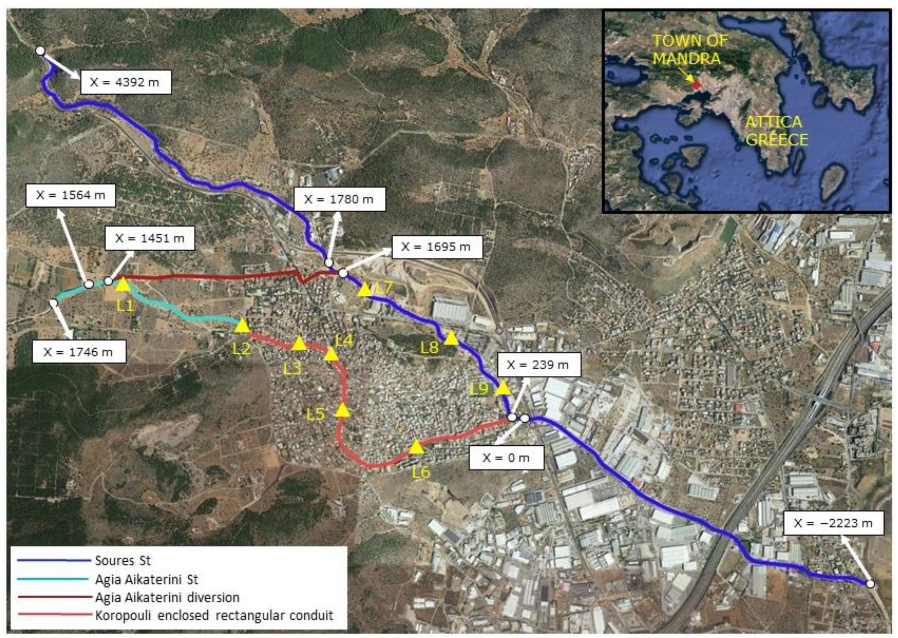
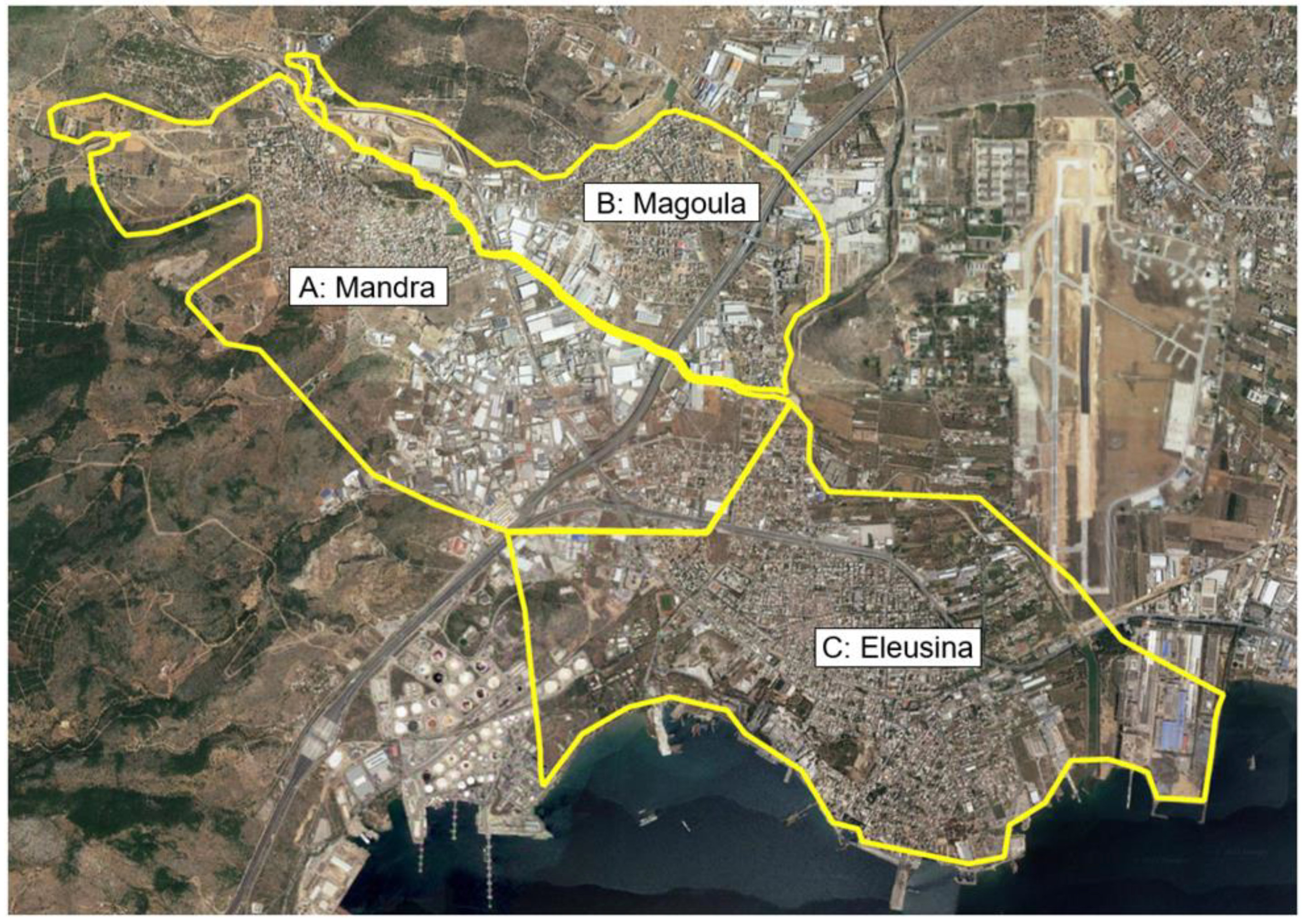
2.1. The Area of Study

The town of Mandra is located 22 km northwest of Athens city center, capital of Greece, has a population of around 13,000, and is situated in the western margin of the Thriasio plain. Mandra consists of continuous urban fabric and a neighboring industrial zone which home to large industrial units and a dense road network. The two main streams (St) in Mandra are shown in Figure 1; these are Soures St and Agia Aikaterini St, which drain areas with catchment sizes equal to 23.0 km² and 22.0 km², respectively. In 2017, these streams that pass through the town of Mandra were characterized by significant reductions in their available cross-sectional areas and the occurrence of floods even at low flow rates due to the intensive construction activities in the greater area; these characteristics were one of the main reasons for the disaster that occurred in November 2017 [13]. Immediately after this catastrophic event, flood protection works in Mandra were constructed according to their Final Study performed in 2014 for a design flood having a return period equal to 50 years. The flood protection works include mainly (1) the regulation of Soures St for a length of 1780 m (x = 239–1695 m) for a design flow equal to 91 m³/s and 125 m³/s (x = 0–239 m), and (2) the diversion of Agia Aikaterini St to Soures St via a 1451 m long channel for a design flow equal to 47 m³/s.

2.2. The HEC-RAS 1D/2D Hydrodynamic Model

In the present work, the unsteady HEC-RAS 1D/2D model is used [14]; in the cross-sections of the Soures St and the Agia Aikaterini St the model solves the 1D hydrodynamic equations, while in the 2D potentially flooded areas the model solves the 2D hydrodynamic equations.

The hydrodynamic equations of the 1D and 2D unsteady HEC-RAS model are the shallow water equations (SWE) that can be written as follows:

Continuity

$$\frac{\partial \mathrm{A}}{\partial \mathrm{t}}+\frac{\partial \mathrm{Q}}{\partial \mathrm{x}}=\mathrm{q}$$

(1)

Momentum

$$\frac{\partial \mathrm{Q}}{\partial \mathrm{t}}+\frac{\partial \left(\mathrm{VQ}\right)}{\partial \mathrm{x}}+\mathrm{gA}\left(\frac{\partial {\mathrm{Z}}_{\mathrm{s}}}{\partial \mathrm{x}}+{\mathrm{S}}_{\mathrm{f}}\right)=0$$

(2)

where A = total cross-sectional area (L²),

Q = total discharge (L³/T),

t = time (T),

x = distance in the direction of the flow (L),

q = inflow per unit length (L²/T),

V = cross-sectional average flow velocity (L/T),

Z_s = water surface elevation (L),

g = gravitational acceleration (L/T²), and

S_f = friction slope (-).

Continuity

$$\frac{\partial \mathrm{h}}{\partial \mathrm{t}}+\frac{\partial \left(\mathrm{hU}\right)}{\partial \mathrm{x}}+\frac{\partial \left(\mathrm{hV}\right)}{\partial \mathrm{y}}=\mathrm{q}$$

(3)

Momentum

$$\frac{\partial \mathrm{U}}{\partial \mathrm{t}}+\mathrm{U}\frac{\partial \mathrm{U}}{\partial \mathrm{x}}+\mathrm{V}\frac{\partial \mathrm{U}}{\partial \mathrm{y}}=-\mathrm{g}\frac{\partial {\mathrm{Z}}_{\mathrm{s}}}{\partial \mathrm{x}}+\frac{1}{\mathrm{h}}\frac{\partial }{\partial \mathrm{x}}\left({\mathrm{v}}_{\mathrm{t},\mathrm{xx}}\mathrm{h}\frac{\partial \mathrm{U}}{\partial \mathrm{x}}\right)+\frac{1}{\mathrm{h}}\frac{\partial }{\partial \mathrm{x}}\left({\mathrm{v}}_{\mathrm{t},\mathrm{yy}}\mathrm{h}\frac{\partial \mathrm{U}}{\partial \mathrm{y}}\right)-\frac{{\mathsf{\tau }}_{\mathrm{b},\mathrm{x}}}{\mathsf{\rho }\mathrm{R}}$$

(4)

$$\frac{\partial {\mathrm{Z}}_{\mathrm{s}}}{\partial \mathrm{y}}+\frac{1}{\mathrm{h}}\frac{\partial }{\partial \mathrm{x}}\left({\mathrm{v}}_{\mathrm{t},\mathrm{xx}}\mathrm{h}\frac{\partial \mathrm{V}}{\partial \mathrm{x}}\right)+\frac{1}{\mathrm{h}}\frac{\partial }{\partial \mathrm{x}}\left({\mathrm{v}}_{\mathrm{t},\mathrm{yy}}\mathrm{h}\frac{\partial \mathrm{V}}{\partial \mathrm{y}}\right)-\frac{{\mathsf{\tau }}_{\mathrm{b},\mathrm{y}}}{\mathsf{\rho }\mathrm{R}}$$

(5)

where h = water depth (L),

q = source/sink flux term (L/T),

u and v = velocities in the Cartesian directions x and y, respectively (L/T),

g = gravitational acceleration (L/T²),

ν_t,xx and v_t,yy = horizontal eddy viscosity in the x and y directions, respectively (L²/T),

τ_b,x and τ_b,y = bottom shear stresses on the x and y directions, respectively (M/L/T²),

ρ = water density (M/L³), and

R = hydraulic radius (L).

In Equations (4) and (5), the acceleration (or inertia) terms are ignored, i.e., when the flood wave propagating over the floodplain is dominated by the forces of gravity, pressure, and friction, then the diffusion wave equations (DWE) are derived. The application of the DWE ensures a sufficiently accurate solution when the assumptions used for their derivation are fulfilled [15]. Generally, the SWE are recommended for highly dynamic flood waves, such as dam breaches and flash floods, abrupt contractions and expansions, flat sloping river systems (slope less than 0.0002), wave propagation due to rapidly opening or closing of gated structures, or wave run-up on a wall or around bridge piers and buildings, super elevation around bends, etc. [14]. However, even in these cases, it is possible to achieve proper accuracy using the DWE [16].

In Equations (4) and (5), the eddy viscosities can be calculated via the Smagorinsky–Lilly model [17,18] that assumes that the turbulent energy production and dissipation at small scales are in equilibrium:

$${\mathrm{v}}_{\mathrm{t}}={\mathrm{Du}}^{*}\mathrm{h}+{({\mathrm{C}}_{\mathrm{s}}\mathsf{\Delta })}^2\left|\overline{\mathrm{S}}\right|$$

(6)

where v_t = eddy viscosity tensor (L²/T) and

D = diffusion coefficient tensor (-)

$$\mathrm{D}=\left[\begin{array}{cc}{\mathrm{D}}_{\mathrm{xx}}& 0\\ 0& {\mathrm{D}}_{\mathrm{yy}}\end{array}\right]$$

(7)

$${\mathrm{D}}_{\mathrm{yy}}={\mathrm{D}}_{\mathrm{L}}{\sin }^2\mathsf{\phi }+{\mathrm{D}}_{\mathsf{{\rm T}}}{\cos }^2\mathsf{\phi }{\mathrm{D}}_{\mathrm{xx}}={\mathrm{D}}_{\mathrm{L}}{\cos }^2\mathsf{\phi }+{\mathrm{D}}_{\mathsf{{\rm T}}}{\sin }^2\mathsf{\phi }$$

(8)

$${\mathrm{D}}_{\mathrm{yy}}={\mathrm{D}}_{\mathrm{L}}{\sin }^2\mathsf{\phi }+{\mathrm{D}}_{\mathsf{{\rm T}}}{\cos }^2\mathsf{\phi }$$

(9)

D_L = user-defined mixing coefficient in the longitudinal direction (-)

D_T = user-defined mixing coefficient in the transverse direction (-)

Φ = direction of velocity (-)

u* = shear velocity (L/T)

C_s = Smagorinsky coefficient that ranges from 0.05 to 0.2

Δ = (Cell Volume)1/3 (L)

(10)

$\left|\overline{\mathrm{S}}\right|$ = strain rate that is calculated by equation

$$\left|\overline{\mathrm{S}}\right|=\sqrt{2{\left(\frac{\partial \mathrm{U}}{\partial \mathrm{x}}\right)}^2+2{\left(\frac{\partial \mathrm{V}}{\partial \mathrm{y}}\right)}^2+2{\left(\frac{\partial \mathrm{U}}{\partial \mathrm{y}}+\frac{\partial \mathrm{V}}{\partial \mathrm{x}}\right)}^2}$$

(11)

The Smagorinsky–Lilly model is somewhat expensive to compute because it requires significant computation times to calculate the velocity gradients. However, it is physically more accurate, especially in the regions of high shear, for example, close to solid/dry boundaries. In the present work, the default values of HEC-RAS 1D/2D that are C_s = 0.05 and D_L = 0.3 and D_T = 0.1 are adopted.

It is important to note that prior to its application in the present work, the hydrodynamic model was calibrated for the case of the disastrous flood of November 2017 using data derived from post-flood field surveys in the area, including water depth and flood extent (presented by Diakakis et al. [19]). Calibration was performed to determine the values of the Manning roughness coefficient in the 2D areas; see Section 2.3, using a time step equal to approximately 1.0 s to satisfy Courant–Friedrichs–Levy (CFL) condition for stability. The following values of the Manning roughness coefficients were determined: discontinuous urban fabric n = 0.100, industrial or commercial units and public facilities n = 0.100, road and rail networks and associated land n = 0.020, olive groves n = 0.045, complex cultivation patterns/non-irrigated arable land n = 0.035, mixed forest n = 0.120, and sclerophyllous vegetation n = 0.100. A detailed description of the calibration procedure is provided by Mitsopoulos et al. [20].

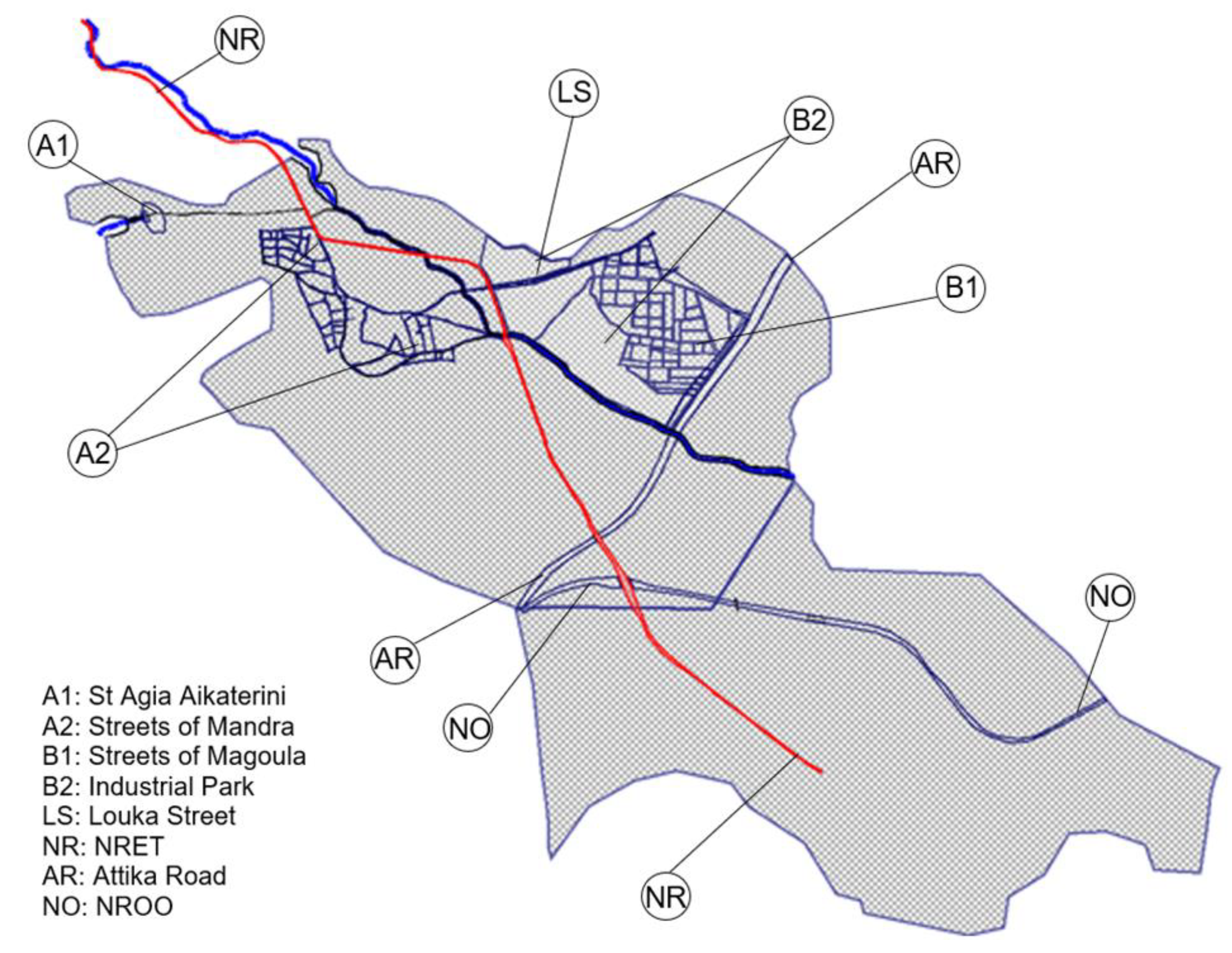
2.3. The Computational Domain and Grid

In Figure 2 the 3 main areas, A, B, and C of the computational domain, are shown with their boundaries; A covers the area at the left (northern) side of Soures St and includes the northern part of the town of Mandra, a part of the town of Magoula, and the industrial park; B covers the area at the right side of Soures St and includes the Agia Aikaterini St and the main part of the town of Mandra; and C extends south to the coast of the Saronic Gulf and includes part of the town of Eleusina and its industrial zone.

The computation domain covers an area of approximately 18.36 km² that includes the total flood inundation areas that is around 3.0 km² [20]. In this domain, the 1D and the 2D numerical grids were constructed using a digital surface model (DSM) of a very high resolution equal to 0.80 m × 0.80 m to capture all hydraulically important features of the area’s surface, including streets, trees, and buildings, that are required for detailed hydrodynamic calculations and were “corrected” via an accurate topographic survey performed during the construction of the flood protection works.

The numerical grid of the computational domain shown in Figure 3 was built as follows. Firstly, the 1D grid in Soures St and Agia Aikaterini St was constructed using cross-sections every approximately 20–50 m with the required refinements where needed. Secondly, the “main mesh” of the 2D computational domain was built with typical dimensions that ranged from 50 m × 50 m to 20 m × 20 m. Thirdly, grid refinement was performed in the areas of interest which are mainly the residential and industrial regions of the towns of Mandra and Magoula, and the streets/roads along which the flood wave that occurred in November 2017 passed; the refinement areas are the following:

• A1: Along Agia Aikaterini St.
• A2: Along the main streets of the residential area of the town of Mandra.
• B1: Along the main streets of the residential area of the town of Magoula.
• B2: Along the industrial park of the town of Mandra.
• NR: Along the National Road Eleusina-Thebes (NRET).
• NO: Along the National Road Olympia (NRO).
• AR: Along the Attica Road.
• LS: Along the Louka Street.

In the refinement areas, A1, B2, LS, AR, and NO, a numerical mesh was employed with dimensions 10 m × 10 m, while in areas A2, B1, and NR we used a finer grid that ranged from 5 m × 5 m to 2 m × 2 m.

2.4. Scenarios of Calculations

Calculations were performed for 8 scenarios, whose characteristics are shown in

Table 1. Characteristics the eight scenarios.

Scenario	Dimensions of Main Mesh (m × m)	Dimensions of Mesh in A2, B1, and NR (m × m)	Dimensions of Mesh in A1, B2, NO, AR, and LS (m × m)	Number of Control Volumes Area A	Number of Control Volumes Area B	Number of Control Volumes Area C	Total Number of Control Volumes	Computational Time (min)
DWE-1	50 × 50	5 × 5	10 × 10	18,423	19,564	5982	43,969	42.05
DWE-2	40 × 40	5 × 5	10 × 10	19,630	20,358	7617	47,605	44.97
DWE-3	20 × 20	5 × 5	10 × 10	30,778	26,314	21,859	78,951	67.40
DWE-4	20 × 20	2 × 2	10 × 10	46,890	26,314	21,859	95,063	74.47
SWE-1	50 × 50	5 × 5	10 × 10	18,423	19,564	5982	43,969	66.87
SWE-2	40 × 40	5 × 5	10 × 10	19,630	20,358	7617	47,605	77.83
SWE-3	20 × 20	5 × 5	10 × 10	30,778	26,314	21,859	78,951	107.33
SWE-4	20 × 20	2 × 2	10 × 10	46,890	26,314	21,859	95,063	126.72

; for the 4 scenarios denoted as SWE-1 to SWE-4 the SWE were solved, while for the 4 scenarios denoted as DWE-1 to DWE-4 the DWE were solved.

In Mitsopoulos et al. [20], the scenario SWE-4 was chosen to successfully calibrate/validate the HEC-RAS 1D/2D model for the flash flood in November 2017, without the flood protection works and after having performed a grid sensitivity analysis. Thus, in the present work, the scenario SWE-4 is considered as the “best” scenario and calculations are performed for the remaining 7 scenarios attempting to reduce the computational time via (i) the use of the approximated DWE and (ii) the refinement of the meshes, as shown in Table 1.

3. Results and Discussion

3.1. Calculated Maximum Water Depths and Velocities

In Figure 4 and Figure 5, the calculated maximum water elevations are shown for the scenarios using SWE and DWE, respectively, along Koropouli Street which is the main street of Mandra that suffered severe flooding during the flood of November 2017. In Figure 6, the calculations of the “best” scenario SWE-4 are compared with its corresponding DWE-4 using DWE. Moreover, in Figure 7, the calculated hydrographs for the water depth and flow rate are shown indicatively in the cross-section that passes through the monitoring location L5.

From Figure 4, Figure 5, Figure 6 and Figure 7 and the calculations, the following conclusions are derived:

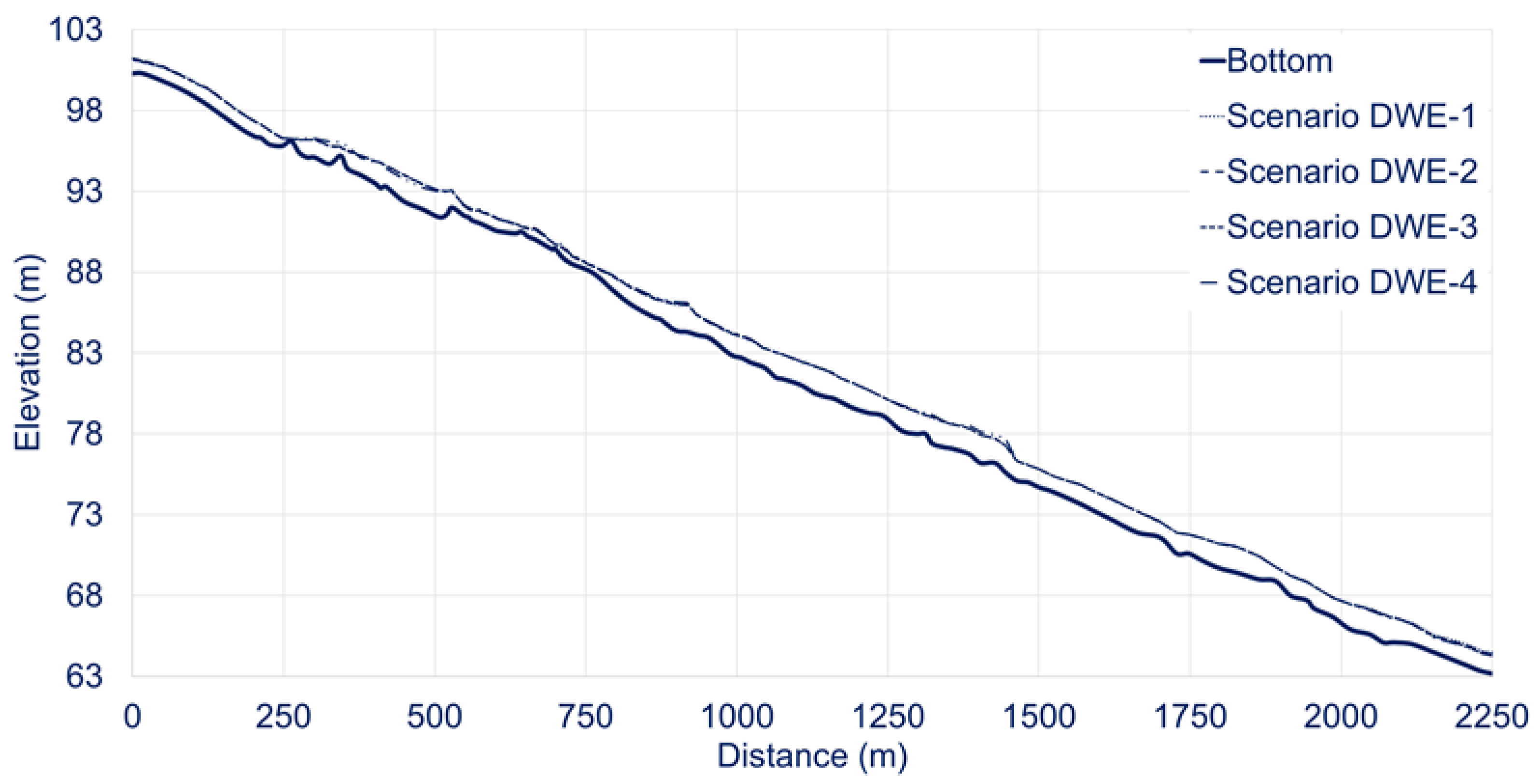
• Calculated water depths for the scenarios DWE-1, DWE-2, and DWE-3 do not show significant differences from the DWE-4; the calculated RMSE was around 9%. Thus, practically, a relatively coarse grid DWE-1 can be used for the calculations using DWE.
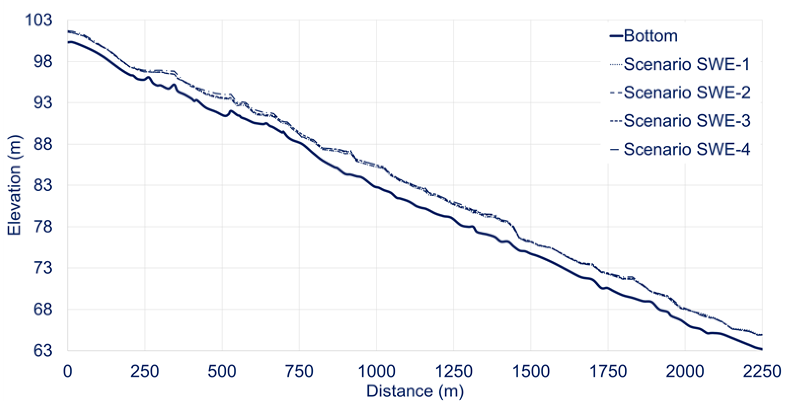
• Calculated water depths for the scenarios SWE-1, SWE-2, and SWE-3 show greater differences from the SWE-4 than the corresponding DWE scenarios; the calculated RMSE ranges from 9% to 16%. Thus, calculations with SWE require much finer grids that should be determined after performing grid independence calculations for the specific case under examination.
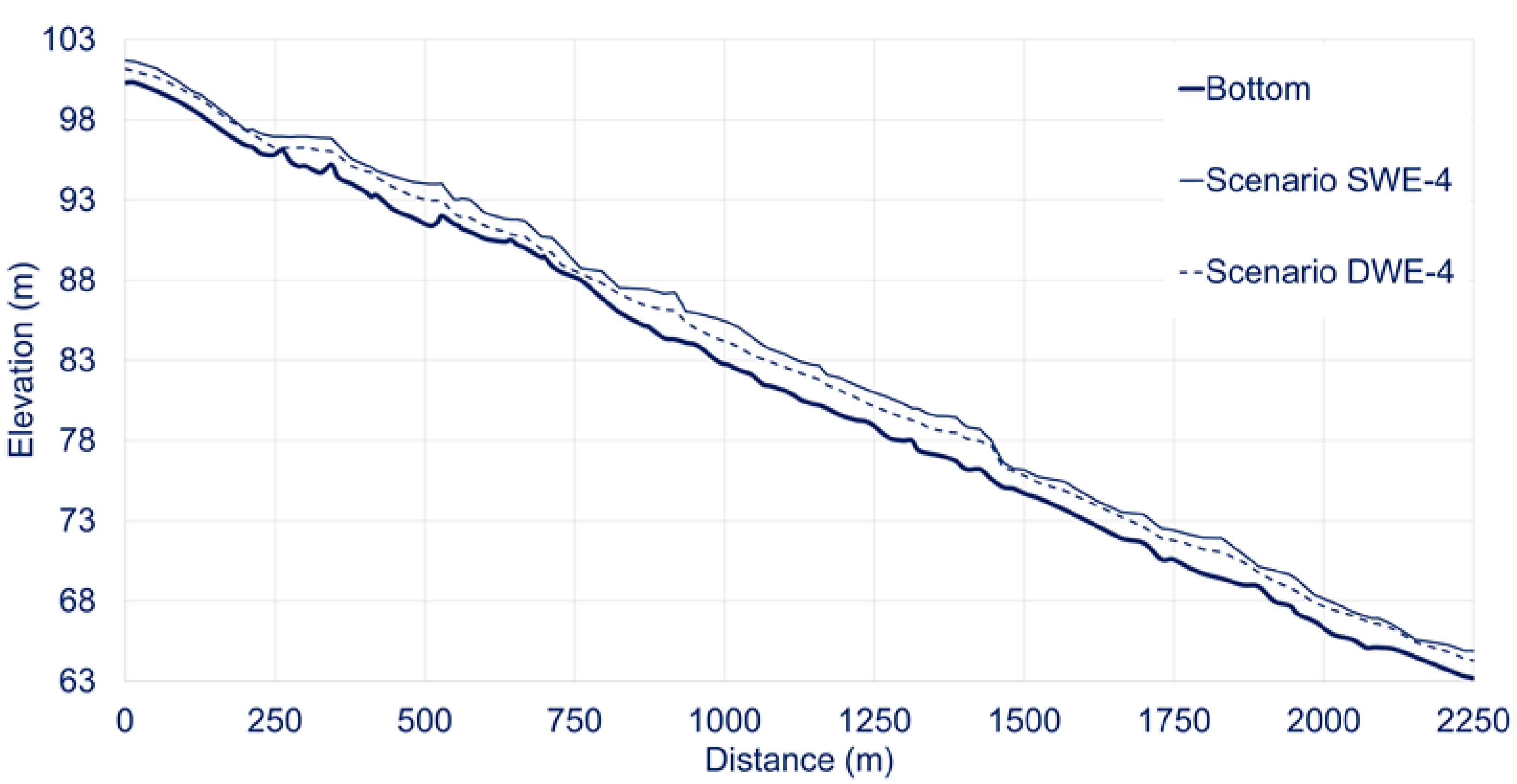
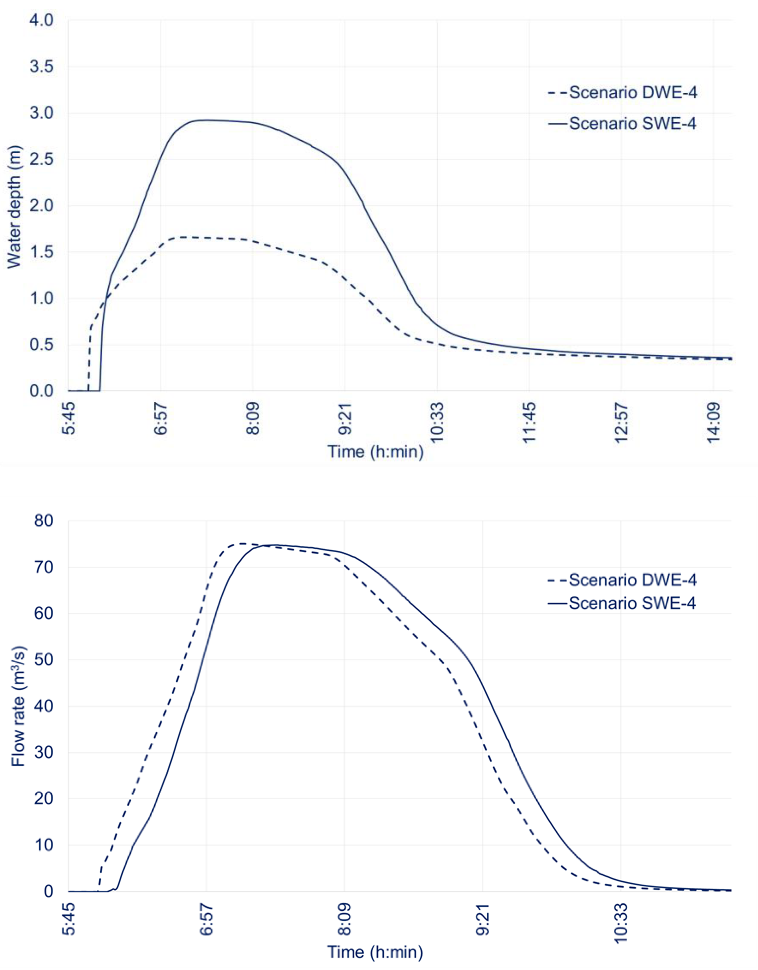
• Calculated maximum water depths using DWE are equal to 60% to 65% of the corresponding values using SWE, i.e., the DWE significantly underestimated water depths.

3.2. Calculated Inundation Areas

Figure 8 and

Table 2. Extent of the total inundation area (km²) and differences between various scenarios (%).

Scenario	Inundation Area	Difference between Corresponding Scenarios (DWE-SWE/SWE)	Difference from Scenario DWE-4	Difference from Scenario SWE-4
DWE-1	2.63	−5.9%	−3.1	-
DWE-2	2.64	−3.0%	−2.8	-
DWE-3	2.72	−7.6%	0.2	-
DWE-4	2.72	−7.9%	0.0	-
SWE-1	2.80	5.9%	-	−5.2
SWE-2	2.72	3.0%	-	−4.5
SWE-3	2.95	7.6%	-	−0.1
SWE-4	2.95	7.9%	-	0.0

show the main characteristics of the calculated inundation areas from which the following conclusions are derived:

• Calculated total inundation areas for the scenarios DWE-1, DWE-2, and DWE-3 show small differences (less than 3.1%) from the DWE-4.
• Calculated total inundation areas for the scenarios SWE-1, SWE-2, and SWE-3 that use SWE also show small differences (less than 5.2%) from the SWE-4, which however, are higher than the corresponding DWE scenarios.
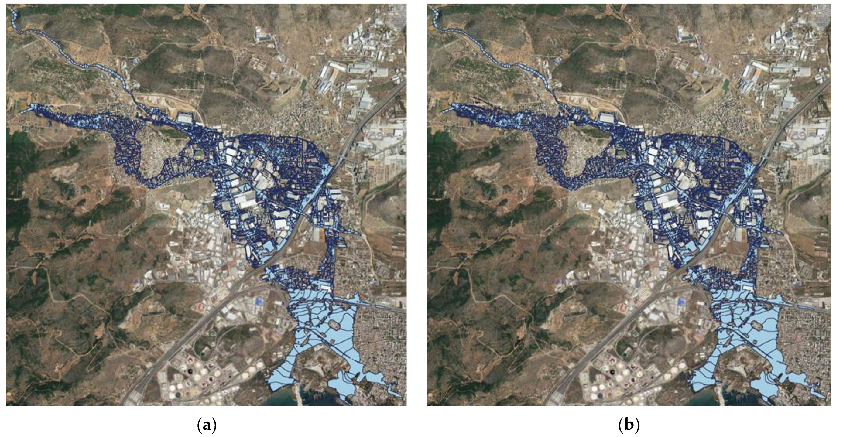
• Calculated total inundation areas using the SWE are larger than those calculated using the DWE by approximately 4.9–7.9%; the higher values were observed for the finer grids.

3.3. Calculated Flood Arrival Times

The calculated flood arrival times at the nine monitoring locations (shown in Figure 1) are shown in

Table 3. Flood arrival times at the eight monitoring locations.

SCENARIO	L1	L2	L3	L4	L5	L6	L7	L8	L9
	Agia Aikaterini St						Soures St
DWE-1	5:22	5:40	5:52	6:05	6:02	6:14	7:23	7:06	7:40
DWE-2	5:22	5:42	5:51	6:04	6:00	6:13	7:19	6:57	7:35
DWE-3	5:22	5:40	5:52	6:01	6:02	6:14	7:15	6:55	7:28
DWE-4	5:22	5:40	5:50	6:01	6:02	6:14	7:15	6:55	7:27
SWE-1	5:10	5:34	5:44	6:00	6:01	6:16	7:21	7:02	7:40
SWE-2	5:22	5:41	5:48	6:02	6:06	6:19	7:20	7:03	7:33
SWE-3	5:22	5:40	5:52	6:05	6:10	6:22	7:18	7:02	7:35
SWE-4	5:22	5:40	5:52	6:05	6:10	6:22	7:18	7:02	7:35

. In the present work, the flood arrival time at a specific location is defined as the required time for the water depth to reach 0.30 m; this value is used in the Flood Risk Management Plans in Greece. Moreover, this depth is generally considered as safe for vehicles, people, and buildings [21]. Table 3 shows the following:

• For the DWE scenarios, the flood arrives faster than in the SWE scenarios due to the generally lower water velocities and higher water depths predicted by the SEW scenarios. The delays of the SWE scenarios range from 0 to 4 min in Agia Aikaterini St and from 3 to 8 min for Soures St.
• Calculated flood arrival times generally show an independence of the grid size for the scenarios with the two finer grids, except these of the very coarse grids, DWE-1 and SWE-1, that show significant differences from the finest grids that range from −9 min (earlier arrival) to +5 min (later arrival-delay) for the SWE and up to 13 min (delay) for the DWE.

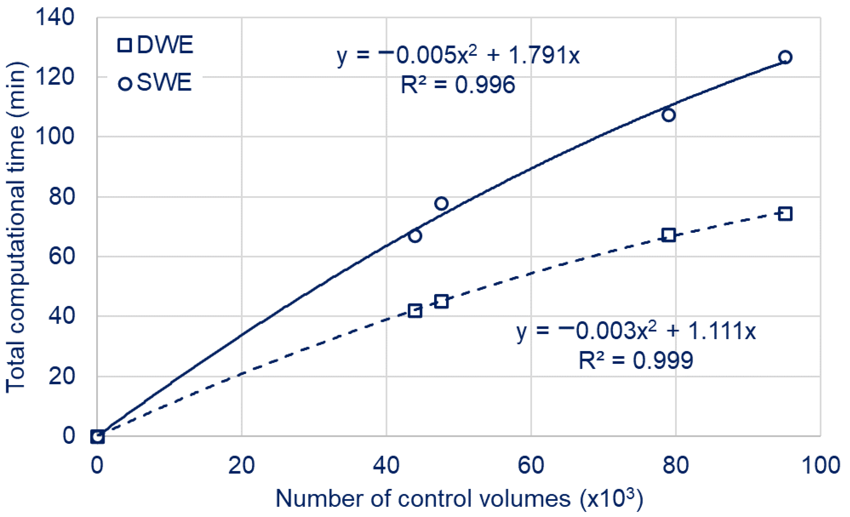
3.4. Computational Times

In Figure 9, the variation in the computation time is shown with the total number of control volumes (noted as y and x, respectively, in the equation shown in Figure 9) and the corresponding regression equations (where R is the regression coefficient) that practically depicts an excellent agreement with the calculations. Generally, for the computational grids examined, the total computation times with SWE was longer by 60–70% than the calculations with DWE.

3.5. Discussion

Overall, this study explored the impact of different computation grid resolutions and of the use of shallow water equations (SWE) versus diffusion wave equations (DWE) in computational time in 2D hydraulic modeling. Through testing of different calculation scenarios, the present study quantifies the effects of the above factors to determine the optimum combination of the minimum grid size and the most appropriate type of equations, i.e., SWE or DWE. The first difference that is immediately observed is that the calculated maximum water depths using DWE in the main streets of Mandra are equal to 60% to 65% of the corresponding values using SWE. This underestimation of water depths by the DWE that is due to the inertial effects was also noticed by other researchers; for example, Hunter et al. [22] applied various models to a 1.0 km × 0.4 km urban catchment within the city of Glasgow, Scotland, UK, to simulate a flood event that occurred at this site on 30 July 2002 and observed that the DWE predict values of water depths up to 5 cm lower than the SWE.

Subsequently, the calculated maximum water velocities in the main streets of Mandra using DWE are significantly higher, being about two-times (maximum = 5 times) higher than the corresponding velocities using SWE. This behavior is ultimately due to neglecting the local acceleration (changes in velocity with respect to time) and convective acceleration (changes in velocity with respect to distance) terms; these two terms are extremely important in order to accurately model rapidly rising flood waves [14]. It is noted that these large differences between the two methods are observed in the main streets of Mandra, where a relatively small number of Manning roughness coefficients is used (n = 0.02) or, in other words, the friction effects are not particularly pronounced. When the flood wave passes through residential areas with relatively high roughness coefficients (n = 0.10–0.20) such as gardens, then these differences become less pronounced due the strong effect of the friction terms; calculated maximum water depths and flow velocities show differences that are less than 3–8%. Thus, if the scope of the calculations is to accurately predict the water depths and flow velocities in regions of relatively low friction, then the solution of the DWE is not recommended; this was also noted by Liang et al. [9], who stated that accurate prediction of hydrodynamics is beyond the scope of DWE.

Due the higher water velocities of the DWE calculations, the flood wave arrives at the monitoring locations faster, by 0–4 min in Agia Aikaterini St and by 3–8 min in Soures St, than the SWE calculations. Moreover, the calculated total inundation areas solving the DWE are smaller by up to 7.9% than these solving the SWE, i.e., the DWE underestimates the inundation area; this is due to the more extensive spreading of the flood wave when the SEW are solved and the acceleration terms are taken into account. This higher spreading was also observed by Hunter et al. [22] who noted that, due to the inertial effects of the SWE, the water has sufficient momentum to overtop bounding topography and continue further, thus, extending the inundation area further than the DWE model. Thus, from the early warning point of view and taking into account that the total computational times of the DWE scenarios are 58.8–62.5% lower than the corresponding SWE, the use of DWE to provide a T4 (flood inundation forecasting) service can be considered as adequate to predict the extend of inundation areas, in spite of their expected underestimation. Moreover, calculations using DWE can be considered as conservative in the calculation of the flood arrival times, although insufficient to accurately model water depths and velocities. Regardless, if the approximation of DWE is adopted in an EWS, the grid independence of the calculations should be ensured. Undoubtedly, if the expected leading times permit the use of SWE, they should definitely be used.

4. Conclusions

In this work, we attempt to answer the following research question, “what are (i) the minimum required computation grid and (ii) the form of hydrodynamic equations (SWE or DWE) in 2D modeling to minimize the computational time while maintaining an acceptable level of error in the prediction of water depths, the flood arrival times, and the extent of flood inundated areas?”. We applied the HEC-RAS 1D/2D model to simulate the disastrous flash flood in Mandra, Attica, Greece, in November 2017 for eight scenarios that involved (i) various grid sizes and (ii) the use of the SWE or the DWE. From these simulations we derived the following conclusions: (i) calculated water depths using the DWE were equal to 60–65% of the corresponding water depths using SWE, i.e., the DWE significantly underestimated water depths; (ii) calculated total inundation areas using the SWE were larger than the corresponding inundation areas using the DWE by approximately 4.9–7.9%; these differences can be considered as acceptable; and (iii) the total computation times using the SWE that ranged from 67 to 127 min were 60–70% longer than the computation times using the DWE. The use of DWE can be considered as adequate to predict the extend of inundation areas when the scope of modeling is to provide a T4 (flood inundation forecasting) despite the expected deficiencies (i.e., underestimated water depths, overestimated flow velocities, and earlier arrival of flood wave). However, for the accurate prediction of water depths and flow velocities in regions of relatively low friction, the SWE are recommended, especially when leading times permit their use. Nevertheless, it is always useful to follow the practical sequence: “(1) solve with the SWE, (2) repeat with the DWE, (3) compare the results of (1) and (2), and (4) decide”.

References

1. Ma, M.; He, B.; Wan, J.; Jia, P.; Guo, X.; Gao, L.; Maguire, L.W.; Hong, Y. Characterizing the Flash Flooding Risks from 2011 to 2016 over China. Water 2018, 10, 704. [Google Scholar] [CrossRef] [Green Version]
2. Ohtsuki, K.; Itsukushima, R.; Sato, T. Feasibility of Traditional Open Levee System for River Flood Mitigation in Japan. Water 2022, 14, 1343. [Google Scholar] [CrossRef]
3. Kurki-Fox, J.J.; Doll, B.A.; Line, D.E.; Baldwin, M.E.; Klondike, T.M.; Fox, A.A. Estimating Changes in Peak Flow and Associated Reductions in Flooding Resulting from Implementing Natural Infrastructure in the Neuse River Basin, North Carolina, USA. Water 2022, 14, 1479. [Google Scholar] [CrossRef]
4. Jubach, R.; Tokar, A.S. International Severe Weather and Flash Flood Hazard Early Warning Systems—Leveraging Coordination, Cooperation, and Partnerships through a Hydrometeorological Project in Southern Africa. Water 2016, 8, 258. [Google Scholar] [CrossRef] [Green Version]
5. UNISDR. Terminology: Basic Terms of Disaster Risk Reduction. 2004. Available online: https://www.unisdr.org/2004/wcdr-dialogue/terminology.htm (accessed on 12 February 2022).
6. Mitsopoulos, G.; Diakakis, M.; Panagiotatou, E.; Sant, V.; Bloutsos, A.; Lekkas, E.; Baltas, E.; Stamou, A.I. Do flood protection works always reduce risk? The case of the 2017 flash flood in Mandra, Attica, Greece. Water, 2022; submitted. [Google Scholar]
7. World Meteorological Organization. WMO Manual on Flood Forecasting and Warning WMO-No. 1072; WMO: Geneva, Switzerland, 2011; ISBN 978-92-63-11072-5. [Google Scholar]
8. Brunner, G. HEC-RAS River Analysis System, 2D Modeling User’s Manual, Version 6.0; USACE CEC: Davis, CA, USA, 2021. [Google Scholar]
9. Liang, Q.; Du, G.; Hall, J.W.; Borthwick, A.G. Flood inundation modeling with an adaptive quadtree grid shallow water equation solver. J. Hydraul. Eng. 2008, 134, 1603–1610. [Google Scholar] [CrossRef]
10. Hardy, R.J.; Bates, P.D.; Anderson, M.G. The importance of spatial resolution in hydraulic models for floodplain environments. J. Hydrol. 1999, 216, 124–136. [Google Scholar] [CrossRef]
11. Bomers, A.; Schielen, R.M.J.; Hulscher, S.J. The influence of grid shape and grid size on hydraulic river modelling performance. Environ. Fluid Mech. 2019, 19, 1273–1294. [Google Scholar] [CrossRef] [Green Version]
12. Horritt, M.S.; Bates, P.D. Effects of spatial resolution on a raster-based model of flood flow. J. Hydrol. 2001, 253, 239–249. [Google Scholar] [CrossRef]
13. Stamou, A. The Disastrous Flash Flood of Mandra in Attica-Greece and Now What? Civ. Eng. Res. J. 2018, 6, 555677. [Google Scholar] [CrossRef] [Green Version]
14. Brunner, G. HEC-RAS River Analysis System, Hydraulic Reference Manual, Version 6.0; USACE CEC: Davis, CA, USA, 2021. [Google Scholar]
15. Cimorelli, L.; Cozzolino, L.; D’Aniello, A.; Pianese, D. Exact solution of the Linear Parabolic Approximation for flow-depth based diffusive flow routing. J. Hydrol. 2018, 563, 620–632. [Google Scholar] [CrossRef]
16. Moussa, R.; Bocquillon, C. On the use of the diffusive wave for modeling extreme flood events with overbank flow in the floodplain. J. Hydrol. 2009, 374, 116–135. [Google Scholar] [CrossRef]
17. Smagorinsky, J. General Circulation Experiments with the Primitive Equations. Mon. Weather Rev. 1963, 91, 99–164. [Google Scholar] [CrossRef]
18. Deardorff, J. A numerical study of three-dimensional turbulent channel flow at large Reynolds numbers. J. Fluid Mech. 1970, 41, 2–453. [Google Scholar] [CrossRef]
19. Diakakis, M.; Andreadakis, E.; Nikolopoulos, E.I.; Spyrou, N.I.; Gogou, M.E.; Deligiannakis, G.; Katsetsiadou, N.K.; Antoniadis, Z.; Melaki, M.; Georgakopoulos, A.; et al. An integrated approach of ground and aerial observations in flash flood disaster investigations. The case of the 2017 Mandra flash flood in Greece. Int. J. Disaster Risk Reduct. 2019, 33, 290–309. [Google Scholar] [CrossRef]
20. Mitsopoulos, G.; Diakakis, M.; Panagiotatou, E.; Sant, V.; Bloutsos, A.; Lekkas, E.; Baltas, E.; Stamou, A.I. How would an extreme flood have behaved if flood protection works were built?” the case of the disastrous flash flood of November 2017 in Mandra, Attica, Greece. Urban Water J. 2022; in production. [Google Scholar] [CrossRef]
21. Smith, G.P.; Davey, E.K.; Cox, R.J. Flood Hazard. Water Research Laboratory; Technical Report University of New South Wales: Manly Vale, NSW, Australia, 2014. [Google Scholar]
22. Hunter, N.M.; Bates, P.D.; Neelz, S.; Pender, G.; Villanueva, I.; Wright, N.G.; Liang, D.; Falconer, R.A.; Lin, B.; Waller, S.; et al. Benchmarking 2D hydraulic models for urban flooding. In Proceedings of the Institution of Civil Engineers—Water Management; Thomas Telford Ltd.: London, UK, 2008; Volume 161, pp. 13–30. [Google Scholar] [CrossRef] [Green Version]
Figure 1. The area of study with the main streams and the flood protection works; the numbered small triangles denoted as L1 to L9 indicate the monitoring locations where flood arrival times are calculated.
Water 14 02356 g001
Figure 2. The boundaries of the computational domain and the three main areas (Google Maps).
Water 14 02356 g002
Figure 3. The numerical grid in the computational domain.
Water 14 02356 g003
Figure 4. Comparison of water elevations along Koropouli Street for the SWE scenarios.
Water 14 02356 g004
Figure 5. Comparison of water elevations along Koropouli Street for the DWE scenarios.
Water 14 02356 g005
Figure 6. Comparison of water elevations along Koropouli Street for the scenarios SWE-4 and DWE-4.
Water 14 02356 g006
Figure 7. Comparison of hydrographs for the water depth and flow rate in the cross-section that passes through the monitoring location L5.
Water 14 02356 g007
Figure 8. Comparison of inundation areas for scenarios (a) DWE-4 and (b) SWE-4.
Water 14 02356 g008
Figure 9. Comparison of total computational time to number of control volumes for scenarios DWE-4 and SWE-4.
Water 14 02356 g009