
Simulation of Chlorophyll a Concentration in Donghu Lake Assisted by Environmental Factors Based on Optimized SVM and Data Assimilation

1
School of Civil and Hydraulic Engineering, Huazhong University of Science and Technology, Wuhan 430074, China
2
School of Electrical and Electronic Engineering, Huazhong University of Science and Technology, Wuhan 430074, China
*
Author to whom correspondence should be addressed.
Water 2022, 14(15), 2353; https://doi.org/10.3390/w14152353
Submission received: 20 June 2022
/
Revised: 22 July 2022
/
Accepted: 26 July 2022
/
Published: 29 July 2022
(This article belongs to the Section Water Quality and Contamination)
Abstract
:Lake eutrophication is a global water environmental problem and has become a research focus nowadays. Chlorophyll a concentration is an important index in terms of evaluating lake eutrophication. The aim of this study was to build an effective and universal empirical model for simulation of chlorophyll a concentration in Donghu Lake. On the basis of the relationship between chlorophyll a concentration and dissolved oxygen (DO), water temperature (T), total nitrogen (TN), and total phosphorus (TP), models for simulating chlorophyll a concentration were built by using simulated annealing (SA), genetic algorithm (GA), artificial bee colony (ABC), and particle swarm optimization (PSO) to optimize parameters of support vector machine (SVM). Moreover, a collaborative mode (Col-SVM model) was built by introducing data assimilation, and meanwhile, accuracy and universality of the model were studied. Modeling results showed that the application of optimization algorithms and data assimilation improved the performance of modeling based on SVM. Model simulation results demonstrated that the Col-SVM model has high accuracy, decent stability, and good simulation effect; the root mean square error (RMSE), mean absolute percentage error (MAPE), Nash–Sutcliffe efficiency coefficient (NSE), bias, and mean relative error (MRE) between simulated values and observed values were 10.07 μg/L, 0.31, 0.96, −0.050, and 0.15, respectively. In addition, model universality analysis results revealed that the Col-SVM model has good universality and can be used to simulate the chlorophyll a concentration of Donghu Lake at different times. Overall, we have built an effective and universal simulation model of chlorophyll a concentration that provides a new idea and method for chlorophyll a concentration modeling.
1. Introduction
Lake eutrophication is a global water environmental problem [1,2]. Chlorophyll a concentration, as an important index of phytoplankton biomass as well as eutrophication, is of great significance for the study of primary productivity, eutrophication, and algal bloom [3,4]. Therefore, it is necessary to explore rapid and accurate methods to monitor chlorophyll a concentration [5].
The traditional in situ monitoring method is usually used as a method to acquire data as it is time-consuming, cumbersome, and of great space-time limitation [6]. Another category of chlorophyll a monitoring is modeling and simulation, which includes remote sensing inversion based on the special optical properties of chlorophyll a and water quality numerical modeling based on the formation mechanism of eutrophication. With the rapid development and wide application of remote sensing technology, remote sensing inversion has gradually developed into an indispensable method for chlorophyll a monitoring because it is timely, widely covered, and costs relatively little [7,8]. Using in situ chlorophyll a concentration data and various satellite images such as Landsat 8 [9], MODIS [10], and Sentinel-2A [11], remote sensing inversion models have been built that are based on back propagation neural network (BPNN) [12], support vector machine (SVM) [13], extreme learning machine (ELM) [14], and artificial neural network (ANN) [15], and these models have good performance and high accuracy in simulating chlorophyll a concentration of inland water. However, remote sensing inversion has some limitations in monitoring chlorophyll a in lakes. Bad weather and a longer revisit cycle limit the images acquisition and application in time series analysis [16,17]. In addition, remote sensing of medium to small lakes requires moderate (≈300 m) to high (10–30 m) spatial resolution sensors, and the resolution of commonly used and easily available satellite images usually cannot meet the requirements for water quality inversion of a small lake [18,19]. In addition, the inversion model has poor universality and it is only applicable to a specific area as the inland water body has different characteristics of regionality and seasonality [20,21]. Consequently, although there are many studies on the inversion of chlorophyll a concentration in Donghu Lake, there is no universally applicable model so far. Eutrophication is a water pollution phenomenon wherein large quantities of nutrition material such as nitrogen and phosphorus enter the water body, causing the rapid reproduction of algae and other phytoplankton, the decline of dissolved oxygen, the deterioration of water quality, and the destruction of the water ecosystem [22,23,24]. Water quality numerical modeling takes into consideration the complex physical, chemical, and ecological changes of water quality components during the formation of eutrophication, and therefore it can comprehensively and dynamically simulate the migration and transformation of water quality components as well as predict the change rule and development trend [25,26,27]. At present, the worldwide used water quality numerical models include WASP [28,29], EFDC [30,31], Delft3D [32,33], FVCOM [34,35], and MIKE [36,37]. However, adequate data and essential information needs to be collected to realize water quality numerical modeling and simulation of chlorophyll a concentration in lakes. In addition, the modeling process needs to input adequate files and appropriate parameters; the calibration of model parameters is cumbersome, and the operation of model system is complex. When lacking high-resolution satellite images and adequate data, we need to explore a new and effective method to monitor the concentration of chlorophyll a in lakes.
The factors leading to eutrophication differ from one lake to another as a variable environment [38]. However, lake eutrophication is mainly caused by excessive nutrient runoff to the lake [39]. There are many factors affecting the growth and reproduction of algae, such as light, temperature, pH, transparency, and nutrients [40,41]. At the same time, the rapid growth of algae will lead to some changes in lake water quality, such as the increase in chlorophyll a concentration and the decrease in transparency and dissolved oxygen (DO) [42]. Therefore, chlorophyll a concentration in water has a specific biochemical relationship with light, water temperature (T), total nitrogen (TN), total phosphorus (TP), and other physical or chemical environmental factors [43]. Nevertheless, the relationship has rarely been used to establish empirical models to simulate chlorophyll a concentration in lakes. Different from water quality numerical models, empirical models do not need to consider the complex formation mechanism of eutrophication, while it constructs the numerical relationship to realize simulation and prediction based on observed data and the machine learning algorithm.
SVM is a widely used machine learning algorithm that has advantages in solving nonlinear fitting and small sample learning problems [44,45]. Thus, it can be chosen as the method to explore the modeling of chlorophyll a concentration in Donghu Lake. Zhang et al. developed an SVM model for the chlorophyll a estimation of Donghu Lake using in situ chlorophyll a concentration data and synchronous Landsat 8 Operational Land Imager (OLI) images [46]. However, kernel function, kernel function parameters, and penalty factor have a great impact on the fitting effect of a SVM model [47]. Therefore, it is necessary to select the appropriate kernel function and to use the optimization algorithm to optimize the parameters in a SVM model. Furthermore, due to the observation error of observed data and the systematic error of an empirical model, there are uncertainties in the modeling process and error between simulated values of the model and the actual value [48]. Data assimilation is an effective method for dynamic modeling that fuses different observation data into a model to modify the initial conditions, model parameters, and state variables, so as to improve the model prediction value, make it closer to the objective truth value, and reduce the uncertainty of model [49,50]. The introduction of data assimilation can integrate the advantages of different models and data, avoid the uncertainty of single model, and improve model accuracy.
The main objective in this study is to build an effective and universal empirical model based on the relationship between chlorophyll a concentration and environmental factors and use it to simulate the chlorophyll a concentration in Donghu Lake. To improve the accuracy of the model, a variety of optimization algorithms and data assimilation are introduced into the modeling process. The contributions of this work are presented as follows: (a) multiple optimization algorithms are used to optimize parameters of the SVM, and empirical models for chlorophyll a concentration simulation are built on the basis of the relationship between chlorophyll a concentration and environmental factors (DO, T, TN, TP); (b) a collaborative model (Col-SVM model) is constructed to simulate chlorophyll a concentration that is based on SVM models and data assimilation; (c) the accuracy and universality of the Col-SVM model are analyzed and verified, proving that the Col-SVM model has high accuracy as well as good stability and can be used to simulate the chlorophyll a concentration of Donghu Lake at different times.
2. Materials and Methods
2.1. Study Area
Donghu Lake (30°22′–30°40′ N, 114°09′–114°39′ E) is located in the northeast of Wuhan, Hubei Province. It is a typical shallow lake in the middle reaches of the Yangtze River, covering an area of 32 km2 and having a mean depth of 2.16 m with a maximum depth of 4.66 m [51]. Donghu Lake is one of the largest urban lakes in China, being mainly composed of Guozheng Lake, Tangling Lake, Miaohu Lake, Tuanhu Lake, Houhu Lake, and Shuiguo Lake. The average annual water temperature is 16.7 °C, the annual potential evaporation is 1269.6 mm, and the average annual precipitation is 1180 mm. The precipitation is concentrated from April to July, accounting for about 60% of the annual precipitation [52].
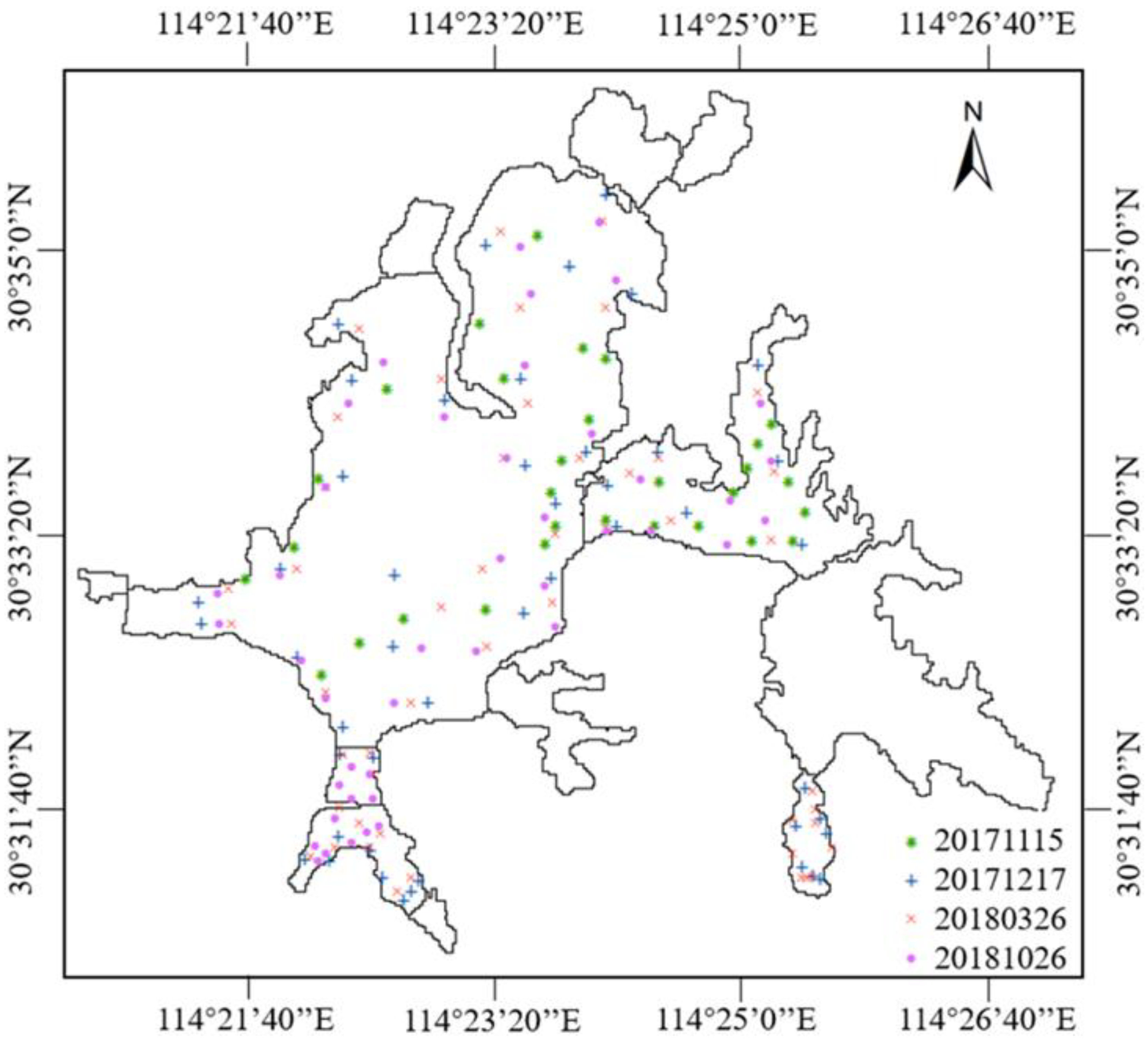
Sampling points were set up in Donghu Lake on 15 November 2017 (20171115), 17 December 2017 (20171217), 26 March 2018 (20180326), and 26 October 2018 (20181026). The sampling points were presented in Figure 1, and the water samples were taken from 0.5 m underwater at every sampling point. DO and T of each water sample were measured on site by a portable water quality detector, and TN and TP were detected by spectrophotometry with water samples sent to a laboratory.
2.2. Support Vector Machine and Optimization Algorithms
2.2.1. Support Vector Machine (SVM)
SVM was proposed by Cortes and Vapnik in 1995 [53]. It can be used for classification [54,55], as well as regression [56,57]. When used for regression modeling, it has advantages in establishing models to solve small-sample, nonlinear, and multidimensional problems [58,59]. In addition, the selection of kernel function, the optimization of penalty parameter, and the kernel parameter determine the applicability and accuracy of the algorithm. The principle of SVM is discussed as follows [60,61]:
Suppose there is a training sample , the regression model can meet the condition that the maximum deviation between and y is below for any , where and are the model parameters to be determined, and is the tolerable deviation. Then, the optimization target of SVM can be formalized as
where refers to the measurement of function flatness, is the regularization constant, is ϵ-insensitive loss function, and can be expessed as
By introducing relaxation variables and , Formula (1) is transformed into
By introducing Lagrange multiplier , Lagrange function is obtained:
At the same time, satisfying the Karush–Kuhn–Tucker (KKT) conditions, the regression model of SVM can be obtained as
where is the kernel function. The sample that can meet the formula is the support vector of SVM. The selection of kernel function and related parameters in the support vector machine has a great influence on the accuracy of the model.
2.2.2. Simulated Annealing (SA)
SA is a random optimization algorithm based on Monte Carlo iterative solution strategy. It was first proposed by N. Metropolis in 1953 [62], and it was successfully introduced into the field of combinatorial optimization by S. Kirkpatrick in 1983 [63]. It has few dependences on problem information, strong universality, and flexibility, and can effectively solve the problem of local optimal solution [64].
2.2.3. Genetic Algorithm (GA)
GA is an algorithm for searching the optimal solution by simulating the genetic mechanism and biological evolution. It was first proposed by John Holland in the 1970s [65]. R. H. Hollstien first used the genetic algorithm for function optimization [66]. It encodes the individuals of practical problems and obtains the optimal solution through a series of operations such as selection, crossover, and mutation. GA has high optimization efficiency, being able to prevent the optimization result from falling into the local optimal solution; at the same time, it has good stability.
2.2.4. Artificial Bee Colony (ABC)
ABC is a swarm intelligence optimization algorithm that was proposed by Karaboga in 2005 [67], being a global optimization algorithm based on swarm intelligence inspired by bees’ behavior of searching for food sources [68]. It has the ability to get out of a local minimum and can be efficiently used for multivariable, multimodal function optimization [69]. In addition, it has fewer control parameters compared to other algorithms and has been successfully implemented for solving complex nonlinear optimization problems and engineering problems with high dimensionality [70].
2.2.5. Particle Swarm Optimization (PSO)
2.3. Modeling and Simulation
2.3.1. Data Pre-Processing
The observed data obtained from four batches of water samples were processed to construct datasets named 20171115, 20171217, 20180326, and 20181026. The data of 43 sampling points on 26 March 2018 were randomly divided into two parts: the data of 28 sampling points were used to build the training dataset, and the data of 15 sampling points were used to build the testing dataset. Chlorophyll a was determined as the output layer and other water quality indexes as the input layer of the model. Mapminmax function was used in MATLAB software to normalize the training dataset and testing dataset.
2.3.2. Modeling
Radial basis function (RBF) was selected as the kernel function, and the chlorophyll a concentration simulation model was built on the basis of the training dataset and SVM. In addition, the model for which the penalty coefficient and kernel parameter were not optimized in the modeling process was named as the SVM model, and it was used as the control group. At the same time, SA, GA, ABC, and PSO were used to optimize the SVM parameters (the penalty coefficient and kernel parameter ). The optimal parameters of the SVM model were obtained through multiple training, and then the SA-SVM model, GA-SVM model, ABC-SVM model, and PSO-SVM model were built. In addition, the error between the simulated and observed values of chlorophyll a concentration in the training process was calculated and analyzed. According to the environmental factor data of the testing dataset, the SVM model, SA-SVM model, GA-SVM model, ABC-SVM model, and PSO-SVM model were used to simulate chlorophyll a concentration. Simulated values were compared with observed values to analyze the accuracy of each model.
The idea of classical data assimilation was to generate an optimal analysis value through the optimization algorithm under the condition of considering the background error and observation error, so that it can more accurately express and describe the real state variable. Model operator, observation operator, error estimation operator, and optimal algorithm are the constituent elements of data assimilation. The goal of data assimilation is to produce the optimal analysis value by optimizing the objective function. The objective function can be expressed as
where J is the objective function; is analysis value; H is observation operator, its function is to transform state variables into observation variables; is the observed value; R is the observed error covariance matrix; B is the background error covariance matrix; and is the background value. On the basis of the idea of data assimilation, the objective function of multi model collaborative simulation can be transformed into
where is the objective function, is analysis values, n is the number of models, is simulated values of different models, and is the simulated error of different models. By calculating the gradient of Equation (7) and making it equal to 0, the optimal analysis value can be obtained. The expression is
where is the weight of simulated values of different models, and is the simulated error of different models. In this study, the root mean square error (RMSE) was used to describe the simulated error of different models.
According to simulated values and error of each model, the data assimilation method was introduced to construct the collaborative model and it was named the Col-SVM model.
2.3.3. Simulation and Model Analysis
Relative error (RE), absolute relative error (ARE), mean relative error (MRE), root mean square error (RMSE), mean absolute percentage error (MAPE), determination coefficient (R), Nash–Sutcliffe efficiency coefficient (NSE), and bias between simulated values and the true values were chosen as evaluation criteria to analyze the performance of the model. Generally, the observed value is used to represent the real value.
RE and ARE measure the error between simulated value and observed value from single group data, while MRE, RMSE, and MAPE measure the overall error between simulated values and observed values from the whole dataset. The smaller the values of RE, ARE, MRE, RMSE, and MAPE, the higher the model accuracy. R measures the linear relationship between the two variables; the absolute value of R is less than or equal to 1, where R < 0 represents negative correlation and R > 0 represents positive correlation. The larger the absolute value of R, the greater the correlation. NSE evaluates the accuracy of the model by comparing simulated values with the mean value of observed values. The closer the NSE value is to 0, the closer simulated value is to the mean value of observed values, and the model accuracy is poor. The closer the NSE value is to 1, the better the accuracy of the model. Bias reflects the error between the output of the model on the sample and the real value, that is, the smaller the bias, the smaller the deviation between the predicted value and the real value, and the higher the fitting degree of the model.
To analyze and evaluate the accuracy of the Col-SVM model, environmental factor data in the dataset 20180326 was used for the Col-SVM model to simulate the chlorophyll a concentration in Donghu Lake, and the error between simulated values and observed values was calculated. Furthermore, simulated values and observed values of chlorophyll a concentration were interpolated by Kriging interpolation method in ArcMap 10.2 software to obtain the chlorophyll a concentration distribution map of the whole Donghu Lake, and the differences between two distribution maps were compared to analyze the accuracy of the Col-SVM model.
The Col-SVM model was used to simulate the chlorophyll a concentration in Donghu Lake at four different times; the simulation results were analyzed, and the error between simulated values and observed values were compared to study the universality at different times.
3. Results and Discussion
3.1. Data and Datasets
Due to the vast water area of Donghu Lake and the limited sampling conditions, the amount of effective water sample data for the four times was different after excluding invalid data. In addition, the valid data constructed four datasets. Each dataset included five indexes: DO, T, TN, TP, and chlorophyll a concentration. The comparison of chlorophyll a concentration in the four datasets is shown in Table 1.
Although the sampling time and sampling point location of the four sampling were different, the chlorophyll a concentration in Donghu Lake had an increasing trend only from the analysis of the chlorophyll a concentration average value.
The dataset of 20180326 was selected for modeling, being randomly divided into the training dataset and testing dataset. The comparison of chlorophyll a concentration in the two datasets is shown in Table 2.
3.2. Parameter Optimization and Modeling
Using the 20180326 dataset, empirical models for chlorophyll a concentration simulation assisted by environmental factors was built on the basis of SVM. When modeling, RBF was selected as the kernel function, and RMSE between simulated values and observed values was selected as the fitness function. To improve the performance of empirical models, the penalty coefficient and kernel parameter of SVM were optimized by SA, GA, ABC, and PSO. The optimized and were obtained by optimization; then, the SA-SVM model, GA-SVM model, ABC-SVM model, and PSO-SVM model were built. At the same time, an empirical model named SVM model was built as the control group. The and of each model are shown in Table 3.
As we can see from Table 3, the optimization of these optimization algorithms changed the parameters of SVM greatly in comparison with the control group. After optimization, the parameters of the SA-SVM model, GA-SVM model, and ABC-SVM model were close, while the parameters of the PSO-SVM model varied greatly compared with the SVM model; at the same time, they also had a large difference from the parameters of the other three optimized models.
The SA-SVM model, GA-SVM model, ABC-SVM model, and PSO-SVM model were used to simulate the chlorophyll a concentration. The RMSE, MAPE, NSE, and bias between simulated values and observed values of chlorophyll a concentration were calculated to compare and analyze the modeling performance of each model both in the training process and testing process. The error comparison of each model in the modeling process is shown in Table 4.
Through the modeling error comparison in Table 4, we see that RMSE and MAPE of four optimized models were all smaller than the SVM model, both in the training and testing process; in other words, the accuracy of empirical models is improved after the SVM parameters have been optimized. Among these models, the RMSE and MAPE of the GA-SVM model both in the training and testing processes were the smallest, which indicates that the GA-SVM model had the highest accuracy and the most stable performance. Furthermore, RMSE and MAPE of four optimized models were reduced in both training and testing processes compared with the SVM model, but those of the PSO-SVM model were not reduced by much. Combined with the result in that the parameters of the PSO-SVM model had a large difference from those of the other three optimized models, it illustrates that optimization of SVM parameters by PSO fell into local optimal value and that the optimized C and γ of the PSO-SVM model were not optimal.
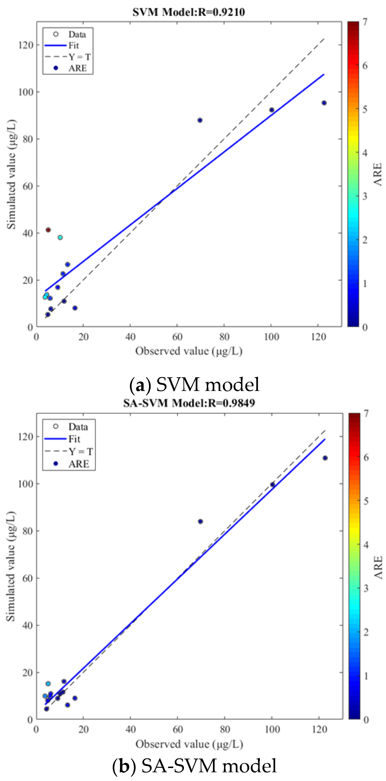
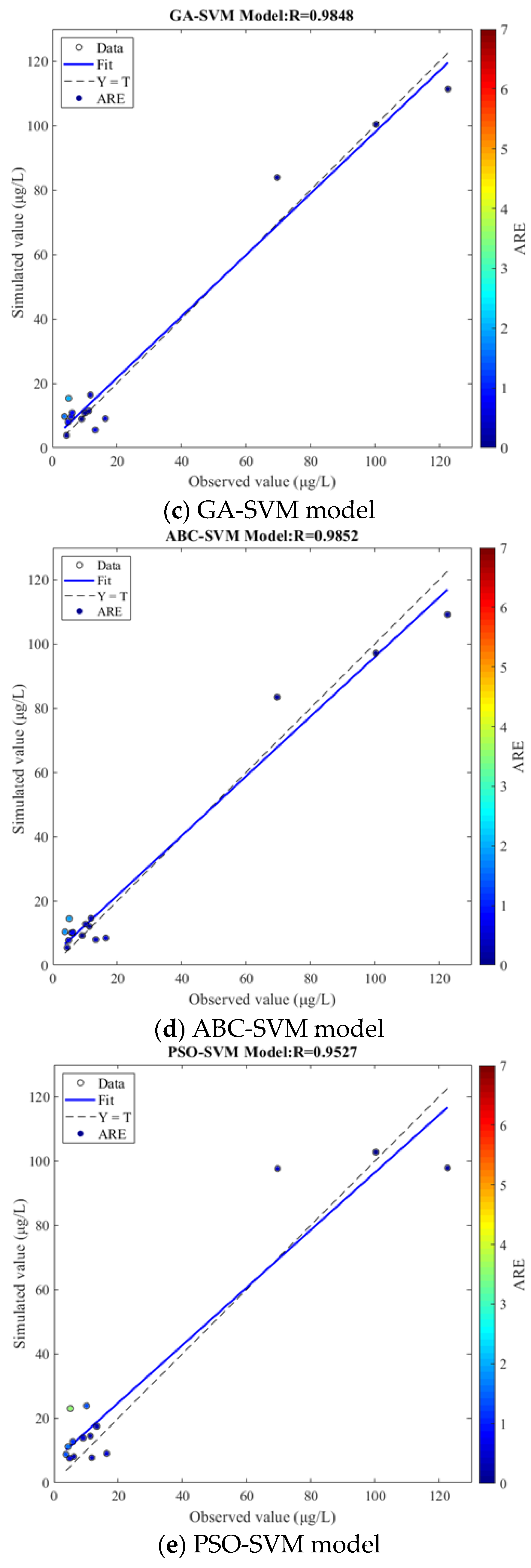
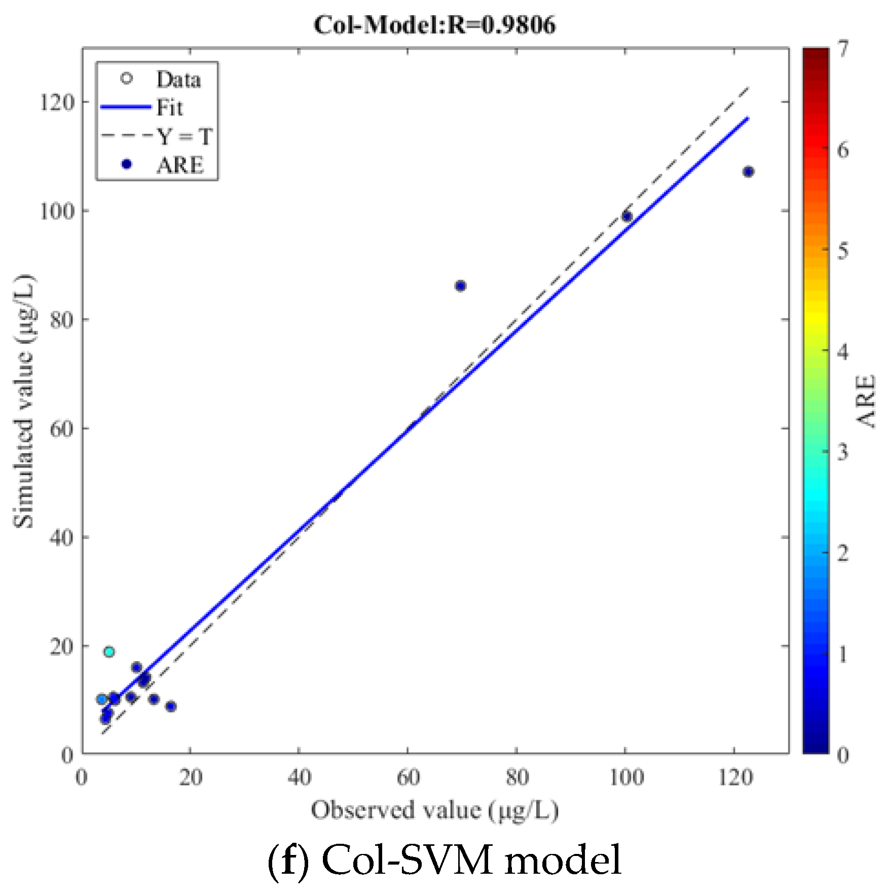
The RMSE in the training process was selected to describe the simulated error of each model. Chlorophyll a concentration simulated values can be obtained by the simulation of the SVM model, SA-SVM model, GA-SVM model, ABC-SVM model, and PSO-SVM model on the basis of the environmental factor data in the testing dataset. According to the simulated error and simulated values of each model, the Col-SVM model can be built by introducing the data assimilation method. Six models were used to simulate the chlorophyll a concentration on the basis of the data of environmental factors in the testing dataset. The testing result comparison of each model is shown in Figure 2.
The results of linear regression analysis between simulated and observed values of chlorophyll a concentration in Figure 2 show that the Rs of each model were 0.9210, 0.9849, 0.9848, 0.9852, 0.9527, and 0.9806. All the Rs were larger than 0.92 in the analysis results of the five models, proving that it is feasible and effective to establish an empirical model based on SVM assisted by environmental factors for chlorophyll a concentration simulation. With the use of optimization algorithms, R of linear regression analysis was improved, and the coincidence degree between regression fitting line (Fit) and reference line (Y = T) was enhanced. At the same time, ARE of sampling points was reduced, and sampling points were relatively closer to the regression fitting line compared with the control group. Furthermore, the analysis results of the Col-SVM model showed that the coincidence degree between Fit and Y = T was high, and the R can reach 0.9806, which was increased by 0.0596 compared with the SVM model. In addition, only a few sampling points deviated from the regression fitting line, and the ARE of all points did not exceed 1.8, except one point with a small observed value. Given all of this, the application of optimization algorithms and data assimilation improved the performance of empirical modeling, and the Col-SVM model showed a good effect on the simulation of chlorophyll a concentration in the testing process.
3.3. Simulation and Accuracy Comparison
On the basis of the environmental factors data in the 20180326 dataset, the SVM model, SA-SVM model, GA-SVM model, ABC-SVM model, PSO-SVM model, and Col-SVM model were used to simulate the chlorophyll a concentration, and the error between simulated values of each model and observed values was analyzed to compare the simulation performance of each model. RMSE, MAPE, NSE, and bias between simulated values and observed values were chosen as evaluation criteria to analyze the simulation effect and accuracy of each model. The simulation error comparison of each model is shown in Table 5.
Table 5 shows that when the SVM model was directly used to simulate chlorophyll a concentration, there was an obvious error between simulated values and observed values, and the RMSE of SVM model reached 19.09 μg/L. Due to the application of optimization algorithms and data assimilation in the SVM model, the RMSE between observed and simulated values of the empirical models was all reduced, showing that the simulation effect of the model on chlorophyll a concentration was improved with the application of optimization algorithms and data assimilation. Among all the optimized models, the RMSE reduction of GA-SVM model was the most, which was decreased by 9.48 μg/L, and that of PSO-SVM model was the least, which was decreased by 0.98 μg/L compared with the SVM model. For the Col-SVM model, its RMSE, MAPE, NSE, and bias were 10.07 μg/L, 0.3132, 0.9577, and −0.0502, respectively, and its RMSE decreased by 9.02 μg/L and MAPE decreased by 0.5345 compared with the SVM model. What is more, the Col-SVM model had the smallest MAPE and the largest NSE, and its NSE was closest to 1 among all the models. In other words, the error between simulated values and observed values was small, the Col-SVM model simulation accuracy was high, and the stability was good. This was because the Col-SVM model integrates the advantages of each SVM model through data assimilation, which ensures the stability of the model output. Taken together, the simulation error analysis result indicates that the application of optimization algorithms is useful in improving the performance of modeling based on SVM and environmental factors; in addition, GA has the best improvement effect. Moreover, data assimilation can not only improve the simulation effect, but also enhance the stability of the model.
3.4. The Performance Analysis of the Col-SVM Model
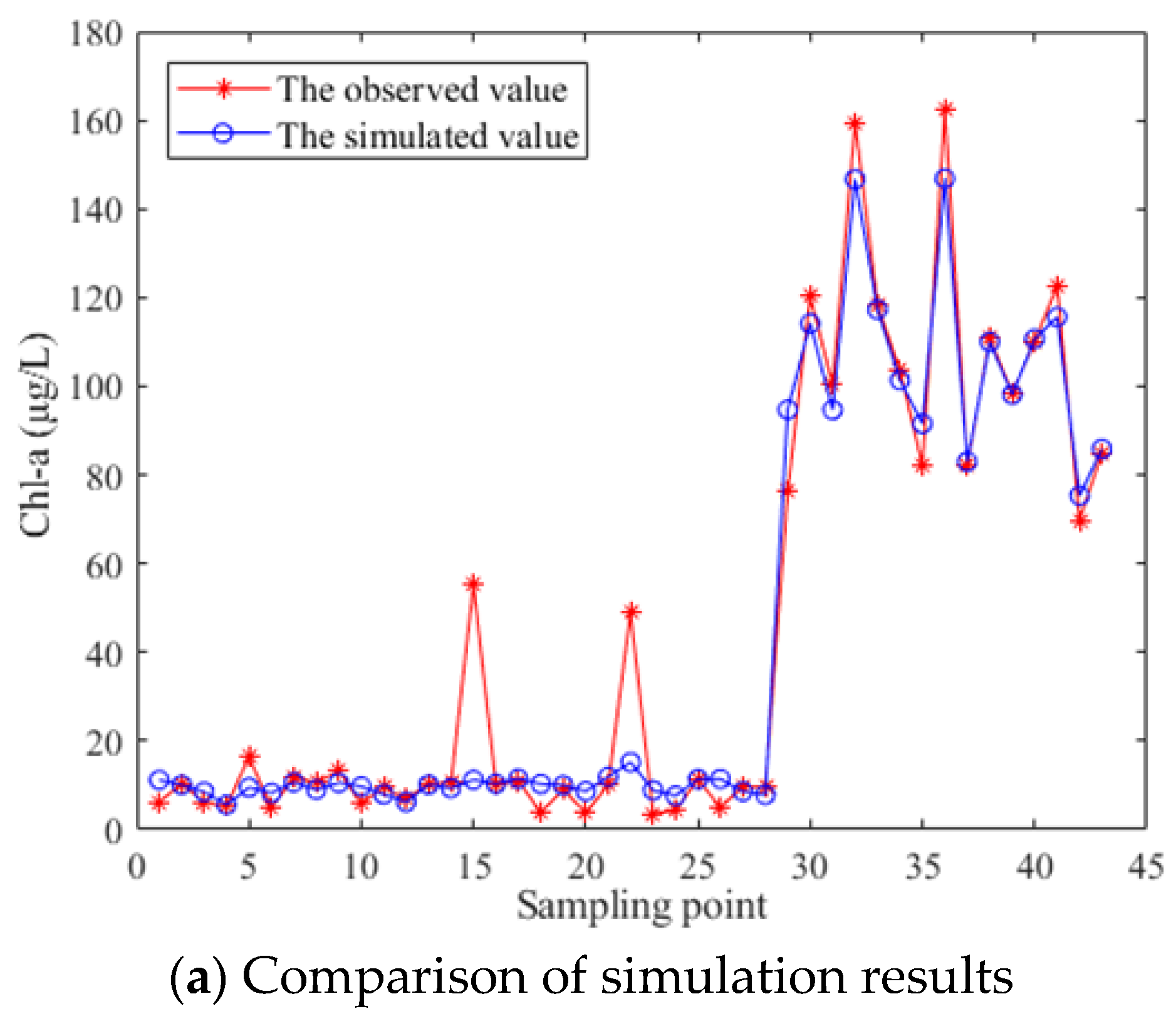
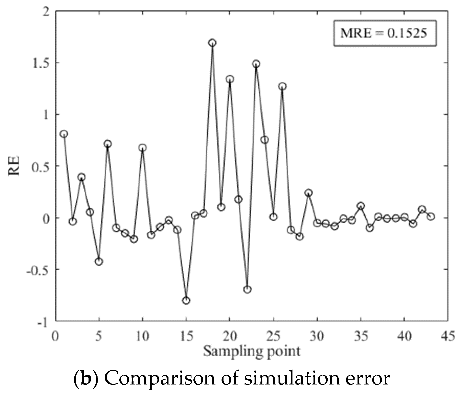
To intuitively show the simulation accuracy of the Col-SVM model, comparison between the chlorophyll a concentration simulated values of the Col-SVM model and observed values at each sampling point was made; moreover, the error at each sampling point was analyzed by means of a chart. The comparison and analysis between simulated values of the Col-SVM model and observed values at each sampling point is shown in Figure 3.
As shown in Figure 3a, simulated values of the Col-SVM model generally coincided with observed values, and simulated values of very few sampling points had obvious deviation from observed values. Figure 3b shows that relative error between simulated values and observed values at sampling points was mainly between −1 and 1, and most of them were between −0.5 and 0.5. In addition, MRE of simulation results was 0.1525. Briefly, the error between simulated values and observed values was not large, and the Col-SVM model had high accuracy and a good simulation effect for chlorophyll a concentration.
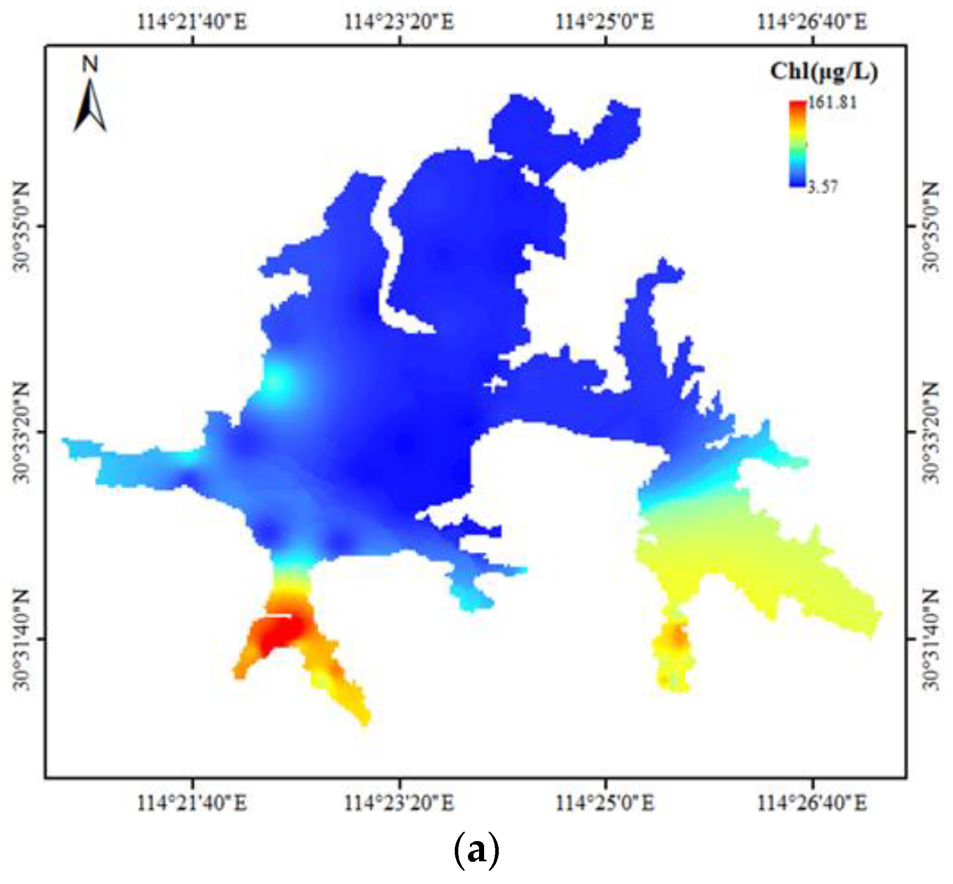
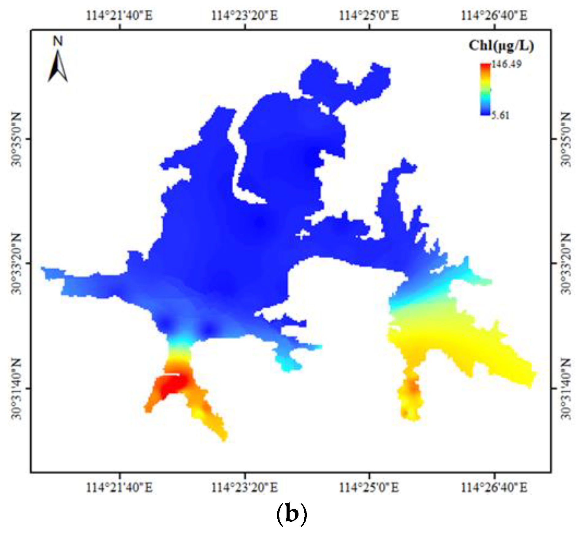
To monitor the overall chlorophyll a concentration of Donghu Lake, it is necessary to convert the known chlorophyll a concentration at sampling points into the chlorophyll a concentration distribution map of the whole lake. The chlorophyll a concentration distribution maps of the whole Donghu Lake were obtained by the spatial interpolation method according to the Col-SVM model simulated values and observed values of chlorophyll a concentration, and they are shown in Figure 4. The simulation effect of the Col-SVM model can be comprehensively analyzed by comparing the differences between the two distribution maps.
It is shown in Figure 4 that the chlorophyll a concentration distribution map based on observed values (a) and simulated values (b) were basically the same. Specifically, distribution of chlorophyll a concentration in the whole Donghu Lake varied greatly, and the areas with high chlorophyll a concentration were distributed in the south and southeast of Donghu Lake on 26 March 2018. Donghu Lake, as one of the largest urban lakes in China, has a vast area of water, but it has been divided into many sub lakes due to human intervention, the water fluidity is poor, and the material transfer and exchange between the sub lakes is slow. Guozheng Lake and Tangling Lake, which are located at the north of Donghu Lake, are the two largest sub lakes of Donghu Lake. They have a large water area and are connected with the Yangtze River and Shahu Lake. Therefore, the water body is flowing, and the pollutants in the water body are easy to diffuse, transfer, transform, and degrade. In addition, the two sub lakes are mainly surrounded by urban communities and natural scenic spots with strict pollution control and good ecological environment protection. As a result, the water quality is good, the eutrophication is not serious, and chlorophyll a concentration is not high. On the contrary, the area of other sub lakes is relatively small, and they have less connection with the external waters; the water flow is slow, and so is the material transfer and transformation. At the same time, most of these sub lakes are long and narrow in shape and have long shorelines around which are many residents, universities, markets, and farmland; as a result, a large amount of domestic sewage and irrigation wastewater containing nutrients are produced around it and are discharged into the water body of these lakes. From this, the concentration of nutrients such as nitrogen and phosphorus in local water bodies becomes extraordinarily high, resulting in water eutrophication and high chlorophyll a concentration. Generally, the simulation result of the Col-SVM model is basically consistent with the actual situation of Donghu Lake. However, there are some differences between Figure 4a,b. First, the concentration ranges of chlorophyll a in the two distribution maps were different. The maximum value in Figure 4a was greater than that in Figure 4b, and the minimum value in Figure 4a is smaller than that in Figure 4b. In addition, there were some differences in the distribution of chlorophyll a concentration in local waters in the two maps. For example, it is shown in Figure 4a that chlorophyll a concentration in Shuiguo Lake and the northwest of Guozheng Lake was higher than that in other waters of Guozheng lake. In the southeast sub lake of Donghu Lake, the chlorophyll a concentration of Miaohu Lake, Houhu Lake, and Yujia Lake increased successively as a whole. However, these differences were not reflected in Figure 4b. The difference between the two distribution maps shows that there were some small errors in the simulation results of chlorophyll a concentration in Donghu Lake. In conclusion, the Col-SVM model shows a good effect on the simulation of chlorophyll a concentration in Donghu Lake, reflecting the real overall distribution of chlorophyll a concentration in Donghu Lake, but the local simulation effect was poor.
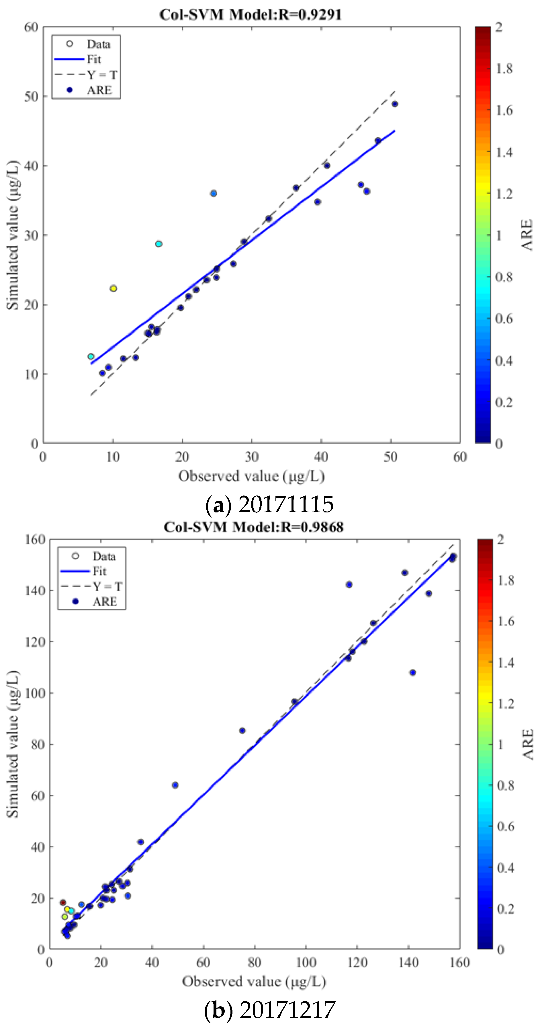
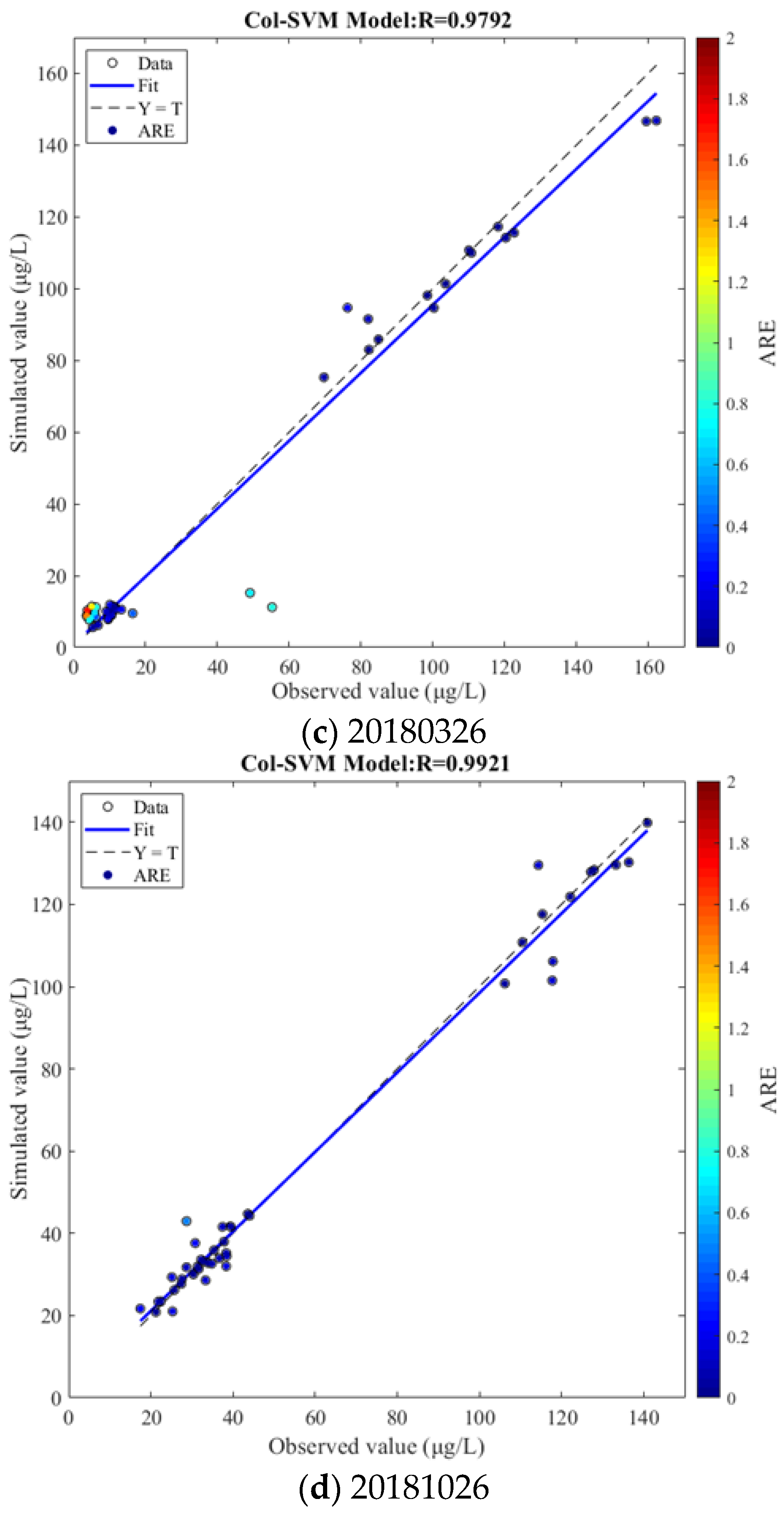
The universality of the Col-SVM model to simulate chlorophyll a concentration of Donghu Lake in the time dimension was verified by using the Col-SVM model and different datasets to simulate chlorophyll a concentration and comparing the error between simulated values and observed values at different times. The comparison between simulated values of the Col-SVM model and observed values of chlorophyll a concentration at different times is shown in Figure 5.
Figure 5 shows the comparison between simulated values and observed values of chlorophyll a concentration at different times, and the results demonstrated that R between simulated values and observed values of chlorophyll a concentration in four different time can reach 0.9291, 0.9868, 0.9792, and 0.9921, and that the determination coefficient between simulated values and observed values of chlorophyll a concentration at four different times all exceeded 0.92, indicating that the ABC-SVM model has good universality. At the same time, it can be found that when the chlorophyll a concentration was low, the simulated values were closer to the observed values, and the simulation effect of the ABC-SVM model was better. When the chlorophyll a concentration was too high, there was a large deviation between the simulation result and the observed values in some sampling points. In general, the difference was not large between simulated values and observed values of chlorophyll a concentration in four time periods, and only a few sampling points had obvious errors. In sum, the Col-SVM model has a good universality in the time dimension and can be used to simulate the chlorophyll a concentration in Donghu Lake at different times.
4. Conclusions
In this study, we used SA, GA, ABC, and PSO to optimize the penalty coefficient and kernel parameter of SVM and built SVM models for chlorophyll a concentration simulation assisted by environmental factors. SVM models (SVM model, SA-SVM model, GA-SVM model, ABC-SVM model, PSO-SVM model) were used to construct the Col-SVM model collaboratively by the introduced data assimilation method. These empirical models were used to simulate the chlorophyll a concentration in Donghu Lake, and the simulation effect of the models was compared and analyzed. The modeling results show that the application of optimization algorithms improved the performance of modeling based on SVM and GA had the best improvement effect. In addition, data assimilation can not only improve the simulation effect, but it can also enhance the stability of the model. The Col-SVM model had good performance in simulating the concentration of chlorophyll a in Donghu Lake, and RMSE, MAPE, NSE, bias, and MRE between simulated values and observed values were 10.07 μg/L, 0.3132, 0.9577, −0.0502, and 0.1525, respectively. Furthermore, R between simulated values and observed values of chlorophyll a concentration at four different times all exceeded 0.92, and Col-SVM model had a good universality in the time dimension and was able to be used to simulate the chlorophyll a concentration in Donghu Lake at different times. In conclusion, the Col-SVM model is a simple and effective empirical model for simulation of chlorophyll a concentration in Donghu Lake.
Author Contributions
X.T.: fieldwork, laboratory work, data analysis, writing and editing; M.H.: simulation suggestion, reviewing, and funding acquisition. All authors have read and agreed to the published version of the manuscript.
Funding
This research was funded by the Science and Technology Project of Central China Branch of State Grid, grant number 5214DK220008, the Science and Technology Project of State Grid Corporation Headquarters, grant number 52170221N00D, the National Key R&D Program of China, grant number No. 2017YFC0405900, and the National Natural Science Foundation of China, grant number No. 51579108.
Institutional Review Board Statement
Not applicable.
Informed Consent Statement
Not applicable.
Data Availability Statement
The data presented in this study are original and available on request from the corresponding author on reasonable request.
Acknowledgments
The authors would like to thank Li Li for her invaluable suggestions and contributions.
Conflicts of Interest
The authors declare no conflict of interest.
References
- Lin, S.; Shen, S.; Zhou, A.; Lyu, H.M. Assessment and management of lake eutrophication: A case study in Lake Erhai, China. Sci. Total Environ. 2020, 751, 141618. [Google Scholar] [CrossRef] [PubMed]
- Zhang, Y.; Liang, J.; Zeng, G.; Tang, W.; Lu, Y.; Luo, Y.; Xing, W.; Tang, N.; Ye, S.; Li, X.; et al. How climate change and eutrophication interact with microplastic pollution and sediment resuspension in shallow lakes: A review. Sci. Total Environ. 2019, 705, 135979. [Google Scholar] [CrossRef] [PubMed]
- Ma, M.; Jia, J.; Hu, Y.; Yang, J.; Lu, Y.; Shi, K.; Gao, Y. Changes in chlorophyll a and its response to nitrogen and phosphorus characteristics over the past three decades in Poyang Lake, China. Ecohydrology 2020, 14, e2270. [Google Scholar] [CrossRef]
- Papenfus, M.; Schaeffer, B.; Pollard, A.I.; Loftin, K. Exploring the potential value of satellite remote sensing to monitor chlorophyll-a for US lakes and reservoirs. Environ. Monit. Assess. 2020, 192, 808. [Google Scholar] [CrossRef] [PubMed]
- Chen, Q.; Guan, T.; Yun, L.; Li, R.; Recknagel, F. Online forecasting chlorophyll-a concentrations by an auto-regressive integrated moving average model: Feasibilities and potentials. Harmful Algae 2015, 43, 58–65. [Google Scholar] [CrossRef]
- Xiang, X.; Lu, W.; Cui, X.; Li, Z.; Tao, J. Simulation of Remote-Sensed Chlorophyll Concentration with a Coupling Model Based on Numerical Method and CA-SVM in Bohai Bay, China. J. Coast. Res. 2018, 84, 1–9. [Google Scholar] [CrossRef]
- Kuhn, C.; Valerio, A.D.; Ward, N.; Loken, L.; Sawakuchi, H.O.; Karnpel, M.; Richey, J.; Stadler, P.; Crawford, J.; Striegl, R.; et al. Performance of landsat-8 and sentinel-2 surface reflectance products for river remote sensing retrievals of chlorophyll-a and turbidity. Remote Sens. Environ. 2019, 224, 104–118. [Google Scholar] [CrossRef] [Green Version]
- Rodriguez-Lopez, L.; Duran-Llacer, I.; Gonzalez-Rodriguez, L.; Abarca-del-Rio, R.; Cardenas, R.; Parra, O.; Martinez-Retureta, R.; Urrutia, R. Spectral analysis using LANDSAT images to monitor the chlorophyll-a concentration in Lake Laja in Chile. Ecol. Inform. 2020, 60, 01183. [Google Scholar] [CrossRef]
- Elangovan, A.; Murali, V. Mapping the chlorophyll-a concentrations in hypereutrophic Krishnagiri Reservoir (India) using Landsat 8 Operational Land Imager. Lakes Reserv. Res. Manag. 2020, 25, 377–387. [Google Scholar] [CrossRef]
- He, J.; Chen, Y.; Wu, J.; Stow, D.A.; Christakos, G. Space-time chlorophyll-a retrieval in optically complex waters that accounts for remote sensing and modeling uncertainties and improves remote estimation accuracy. Water Res. 2020, 171, 115403. [Google Scholar] [CrossRef] [PubMed]
- Saberioon, M.; Brom, J.; Nedbal, V.; Soucek, P.; Cisar, P. Chlorophyll-a and total suspended solids retrieval and mapping using Sentinel-2A and machine learning for inland waters. Ecol. Indic. 2020, 113, 106236. [Google Scholar] [CrossRef]
- He, Y.; Gong, Z.; Zheng, Y.; Zhang, Y. Inland Reservoir Water Quality Inversion and Eutrophication Evaluation Using BP Neural Network and Remote Sensing Imagery: A Case Study of Dashahe Reservoir. Water 2021, 13, 2844. [Google Scholar] [CrossRef]
- Xia, J.; Zeng, J. Environmental factor assisted chlorophyll-a prediction and water quality eutrophication grade classification: A comparative analysis of multiple hybrid models based on a SVM. Environ. Sci. Water Res. Technol. 2021, 7, 1040–1049. [Google Scholar] [CrossRef]
- Peterson, K.T.; Sagan, V.; Sidike, P.; Hasenmueller, E.A.; Sloan, J.J.; Knouft, J.H. Machine learning-based ensemble prediction of water-quality variables using feature-level and decision-level fusion with proximal remote sensing. Photogramm. Eng. Remote Sens. 2019, 85, 269–280. [Google Scholar] [CrossRef]
- Wang, T.; Tan, C.; Chen, L.; Tsai, Y.C. Applying Artificial Neural Networks and Remote Sensing to Estimate Chlorophyll-a Concentration in Water Body. In Proceedings of the 2008 Second International Symposium on Intelligent Information Technology Application, Shanghai, China, 20–22 December 2008; Volume 1, pp. 540–544. [Google Scholar]
- Liu, X.; Xing, Y.; Luo, P. Wetland Plant Extraction Based on the Time Series Landsat NDVI in Dongting Lake Area. For. Resour. Manag. 2017, 4, 103–109. [Google Scholar]
- Wu, M.; Niu, Z.; Wang, C.; Wu, C.; Wang, L. Use of MODIS and Landsat time series data to generate high-resolution temporal synthetic Landsat data using a spatial and temporal reflectance fusion model. J. Appl. Remote Sens. 2012, 6, 063507. [Google Scholar]
- Cao, Z.; Ma, R.; Duan, H.; Pahlevan, N.; Melack, J.; Shen, M.; Xue, K. A machine learning approach to estimate chlorophyll-a from Landsat-8 measurements in inland lakes. Remote Sens. Environ. 2020, 248, 111974. [Google Scholar] [CrossRef]
- Avdan, Z.Y.; Kaplan, G.; Goncu, S.; Avdan, U. Monitoring the Water Quality of Small Water Bodies Using High-Resolution Remote Sensing Data. ISPRS Int. J. Geo-Inf. 2019, 8, 553. [Google Scholar] [CrossRef] [Green Version]
- Keller, P.A. Comparison of two inversion techniques of a semi-analytical model for the determination of lake water constituents using imaging spectrometry data. Sci. Total Environ. 2001, 268, 189–196. [Google Scholar] [CrossRef]
- Palmer, S.C.J.; Kutser, T.; Hunter, P.D. Remote sensing of inland waters: Challenges, progress and future directions. Remote Sens. Environ. 2014, 157, 1–8. [Google Scholar] [CrossRef] [Green Version]
- May, L.; Olszewska, J.; Gunn, I.D.M.; Meis, S.; Spears, B.M. Eutrophication and restoration in temperate lakes. IOP Conf. Ser. Earth Environ. Sci. 2020, 535, 012001. [Google Scholar] [CrossRef]
- Le Moal, M.; Gascuel-Odoux, C.; Menesguen, A.; Souchon, Y.; Etrillard, C.; Levain, A.; Moatar, F.; Pannard, A.; Souchu, P.; Lefebvre, A.; et al. Eutrophication: A new wine in an old bottle? Sci. Total Environ. 2019, 651, 1–11. [Google Scholar] [CrossRef] [PubMed] [Green Version]
- Jiao, J.; Li, P.; Feng, D. Dynamics of water eutrophication model with control. Adv. Differ. Equ. 2018, 2018, 383. [Google Scholar] [CrossRef]
- Vincon-Leite, B.; Casenave, C. Modelling eutrophication in lake ecosystems: A review. Sci. Total Environ. 2019, 651, 2985–3001. [Google Scholar] [CrossRef]
- Gal, G.; Hipsey, M.; Rinke, K.; Robson, B. Novel approaches to address challenges in modelling aquatic ecosystems Preface. Environ. Model. Softw. 2014, 61, 246–248. [Google Scholar] [CrossRef]
- Anagnostou, E.; Gianni, A.; Zacharias, I. Ecological modeling and eutrophication—A review. Nat. Resour. Model. 2017, 30, e12130. [Google Scholar] [CrossRef]
- Wang, X.; Jia, J.; Su, T.; Zhao, Z.; Xu, J.; Wang, L. A Fusion Water Quality Soft-Sensing Method Based on WASP Model and Its Application in Water Eutrophication Evaluation. J. Chem. 2018, 2018, 9616841. [Google Scholar] [CrossRef] [Green Version]
- Seo, D.; Kim, M.; Ahn, J.H. Prediction of Chlorophyll-a Changes due to Weir Constructions in the Nakdong River Using EFDC-WASP Modelling. Environ. Eng. Res. 2012, 17, 95–102. [Google Scholar] [CrossRef] [Green Version]
- Zheng, L.; Wang, H.; Liu, C.; Zhang, S.; Ding, A.; Xie, E.; Li, J.; Wang, S. Prediction of harmful algal blooms in large water bodies using the combined EFDC and LSTM models. J. Environ. Manag. 2021, 295, 113060. [Google Scholar] [CrossRef] [PubMed]
- Tang, T.; Yang, S.; Yin, K.; Zou, R. Simulation of eutrophication in Shenzhen Reservoir based on EFDC model. Hupo Kexue 2014, 26, 393–400. [Google Scholar]
- Liu, Z.; Li, Z.; Hu, L.; Lin, Y.; Chen, Q. Ensemble Kalman filter based data assimilation in the Delft3D-BLOOM lake eutrophication model. Hupo Kexue 2017, 29, 1070–1083. [Google Scholar]
- Liu, S.; Ye, Q.; Wu, S.; Stive, M.J.F. Wind Effects on the Water Age in a Large Shallow Lake. Water 2020, 12, 1246. [Google Scholar] [CrossRef]
- Luo, F.; Gou, H.; Li, R.; Wang, H.; Chen, Z.; Lin, W.; Li, K. Numerical simulation on marine environmental capacity in the open sea area of Northern Jiangsu Province using a three-dimensional water quality model based on FVCOM. Reg. Stud. Mar. Sci. 2021, 45, 101856. [Google Scholar] [CrossRef]
- Yang, Z.; Shao, W.; Ding, Y.; Shi, J.; Ji, Q. Wave Simulation by the SWAN Model and FVCOM Considering the Sea-Water Level around the Zhoushan Islands. J. Mar. Sci. Eng. 2020, 8, 783. [Google Scholar] [CrossRef]
- Kanda, E.K.; Kipkorir, E.C.; Kosgei, J.R. Modelling of nitrates in River Nzoia using MIKE 11. Water Pract. Technol. 2017, 12, 217–223. [Google Scholar] [CrossRef] [Green Version]
- Li, X.; Huang, M.; Wang, R. Numerical Simulation of Donghu Lake Hydrodynamics and Water Quality Based on Remote Sensing and MIKE 21. ISPRS Int. J. Geo-Inf. 2020, 9, 94. [Google Scholar] [CrossRef] [Green Version]
- Karydis, M. Eutrophication Assessment of Coastal Waters based on Indicators: A Literature Review. Glob. Nest J. 2009, 11, 373–390. [Google Scholar]
- Ayele, H.S.; Atlabachew, M. Review of characterization, factors, impacts, and solutions of Lake eutrophication: Lesson for lake Tana, Ethiopia. Environ. Sci. Pollut. Res. 2021, 28, 14233–14252. [Google Scholar] [CrossRef]
- Zhao, X.; Xu, D.; Liu, T.; Long, H.; Zhang, L.; Zhan, C.; Zhang, J.; Liu, X.; Xiao, W. Spatial distribution of chlorophyll-a and its correlation with and water quality indicators in Qingshan Lake. Environ. Chem. 2018, 37, 1482–1490. [Google Scholar]
- Daggett, C.T.; Saros, J.E.; Lafrancois, B.M.; Simon, K.S.; Amirbahman, A. Effects of increased concentrations of inorganic nitrogen and dissolved organic matter on phytoplankton in boreal lakes with differing nutrient limitation patterns. Aquat. Sci. 2015, 77, 511–521. [Google Scholar] [CrossRef]
- Coffin, M.R.S.; Courtenay, S.C.; Pater, C.C.; van den Heuvel, M.R. An empirical model using dissolved oxygen as an indicator for eutrophication at a regional scale. Mar. Pollut. Bull. 2018, 133, 261–270. [Google Scholar] [CrossRef]
- Li, Y.; Yan, X.; Wu, Z.; Liu, Y.; Guo, H.; Zhao, L.; He, B. Quantitative relationship between chlorophyll a and key controlling factors in Four Plateau Lakes in Yunnan Province, China. Acta Sci. Circumstantiae 2015, 35, 402–410. [Google Scholar]
- Cherkassky, V. The Nature of Statistical Learning Theory. IEEE Trans. Neural Netw. 1997, 8, 1564. [Google Scholar] [CrossRef] [Green Version]
- Tang, X.; Huang, M. Inversion of Chlorophyll-a Concentration in Donghu Lake Based on Machine Learning Algorithm. Water 2021, 13, 1179. [Google Scholar] [CrossRef]
- Zhang, T.; Huang, M.; Wang, Z. Estimation of chlorophyll-a Concentration of lakes based on SVM algorithm and Landsat 8 OLI images. Environ. Sci. Pollut. Res. 2020, 27, 14977–14990. [Google Scholar] [CrossRef] [PubMed]
- Xu, Y.; Ma, C.; Liu, Q.; Xi, B.; Qian, G.; Zhang, D.; Huo, S. Method to predict key factors affecting lake eutrophication—A new approach based on support vector regression model. Int. Biodeterior. Biodegrad. 2015, 102, 308–315. [Google Scholar] [CrossRef]
- Vrugt, J.A.; Diks, C.G.H.; Gupta, H.V.; Bouten, W.; Verstraten, J.M. Improved treatment of uncertainty in hydrologic modeling: Combining the strengths of global optimization and data assimilation. Water Resour. Res. 2005, 41, W01017. [Google Scholar] [CrossRef]
- Li, Y.; Li, Y.; Lu, H.; Zhu, L.; Wu, C.; Du, C.; Wang, S. Muti-model Collaborative Retrieval of Chlorophyll a in Taihu Lake Based on Data Assimilation. Huanjing Kexue 2014, 35, 3389–3396. [Google Scholar]
- Cho, K.H.; Pachepsky, Y.; Ligaray, M.; Kwon, Y.; Kim, K.H. Data assimilation in surface water quality modeling: A review. Water Res. 2020, 186, 116307. [Google Scholar] [CrossRef] [PubMed]
- Wang, T.; Wang, Q.; Xia, S.; Yan, C.; Pei, G. Response of benthic algae to environmental conditions in an urban lake recovered from eutrophication. China J. Oceanol. Limnol. 2020, 38, 93–101. [Google Scholar] [CrossRef]
- Peng, Q.; Li, Z.; Deng, X.; Su, M. Nitrogen and phosphorus deposition in urban lakes and its impact factors: A case study of East Lake in Wuhan. Acta Sci. Circumstantiae 2019, 39, 2635–2643. [Google Scholar]
- Cortes, C.; Vapnik, V. Support-Vector Networks. Mach. Learn. 1995, 20, 273–297. [Google Scholar] [CrossRef]
- Bangira, T.; Alfieri, S.M.; Menenti, M.; van Niekerk, A. Comparing Thresholding with Machine Learning Classifiers for Mapping Complex Water. Remote Sens. 2019, 11, 1351. [Google Scholar] [CrossRef] [Green Version]
- Liu, Y.; Wang, H.; Zhang, H.; Liber, K. A comprehensive support vector machine-based classification model for soil quality assessment. Soil Tillage Res. 2016, 155, 19–26. [Google Scholar] [CrossRef]
- Tang, W.; Li, Y.; Yu, Y.; Wang, Z.; Xu, T.; Chen, J.; Lin, J.; Li, X. Development of models predicting biodegradation rate rating with multiple linear regression and support vector machine algorithms. Chemosphere 2020, 253, 126666. [Google Scholar] [CrossRef]
- Park, Y.; Cho, K.H.; Park, J.; Cha, S.M.; Kim, J.H. Development of early-warning protocol for predicting chlorophyll-a concentration using machine learning models in freshwater and estuarine reservoirs, Korea. Sci. Total Environ. 2015, 502, 31–41. [Google Scholar] [CrossRef]
- Kong, X.; Che, X.; Su, R.; Zhang, C.; Yao, Q.; Shi, X. A new technique for rapid assessment of eutrophication status of coastal waters using a support vector machine. J. Oceanol. Limnol. 2018, 36, 249–262. [Google Scholar] [CrossRef]
- Abburu, S.; Golla, S.B. Satellite Image Classification Methods and Techniques: A Review. Int. J. Comput. Appl. 2015, 119, 20–25. [Google Scholar] [CrossRef]
- Noori, R.; Karbassi, A.R.; Ashrafi, K.; Ardestani, M.; Mehrdadi, N.; Bidhendi, G.R.N. Active and online prediction of BOD5 in river systems using reduced-order support vector machine. Environ. Earth Sci. 2012, 67, 141–149. [Google Scholar] [CrossRef]
- Noori, R.; Deng, Z.Q.; Kiaghadi, A.; Kachoosangi, F.T. How Reliable Are ANN, ANFIS, and SVM Techniques for Predicting Longitudinal Dispersion Coefficient in Natural Rivers? J. Hydraul. Eng. 2016, 142, 04015039. [Google Scholar] [CrossRef]
- Steinbrunn, M.; Moerkotte, G.; Kemper, A. Heuristic and Randomized Optimization for the Join Ordering Problem. VLDB J. 1997, 6, 8–17. [Google Scholar] [CrossRef]
- Kirkpatrick, S.; Gelatt, C.D.; Vecchi, M.P. Optimization by Simulated Annealing. Science 1983, 220, 671–680. [Google Scholar] [CrossRef]
- Li, J.; Xia, J.; Zeng, X.; Zeng, J.; Liu, X.; Leng, M.; Sun, L. Survey of multi-objective simulated annealing algorithm and its applications. Comput. Eng. Sci. 2013, 35, 77–88. [Google Scholar]
- Schmitt, L.M. Theory of genetic algorithms. Theor. Comput. Sci. 2001, 259, 1–61. [Google Scholar] [CrossRef] [Green Version]
- Hollstien, R.B. Aritifical Genetic Adaptation in Computer Control Systems. Ph.D. Thesis, University of Michigan, Ann Arbor, MI, USA, 1971. [Google Scholar]
- Karaboga, D.; Basturk, B. A powerful and efficient algorithm for numerical function optimization: Artificial bee colony (ABC) algorithm. J. Glob. Optim. 2007, 39, 459–471. [Google Scholar] [CrossRef]
- Karaboga, D.; Basturk, B. On the performance of artificial bee colony (ABC) algorithm. Appl. Soft Comput. 2008, 8, 687–697. [Google Scholar] [CrossRef]
- Karaboga, D.; Akay, B. A comparative study of Artificial Bee Colony algorithm. Appl. Math. Comput. 2009, 214, 108–132. [Google Scholar] [CrossRef]
- Chen, S.; Fang, G.; Huang, X.; Zhang, Y. Water Quality Prediction Model of a Water Diversion Project Based on the Improved Artificial Bee Colony–Backpropagation Neural Network. Water 2018, 10, 806. [Google Scholar] [CrossRef] [Green Version]
- Kennedy, J.; Eberhart, R. Particle swarm optimization. In Proceedings of the ICNN’95—International Conference on Neural Networks, Perth, Australia, 27 November–1 December 1995; Volume 4, pp. 1942–1948. [Google Scholar]
- Shi, L.; Qin, C. Application of hybrid PSO-RBF neural network in water quality evaluation. J. Saf. Environ. 2018, 8, 353–356. [Google Scholar]
Figure 1.
Distribution of sampling points in Donghu Lake.

Figure 2.
The testing results comparison of each model.


Figure 3.
The performance comparison and analysis of the Col-SVM model at each sampling point.


Figure 4.
The comparison of chlorophyll a concentration distribution map in Donghu Lake. (a) Chlorophyll a concentration distribution map based on observed values. (b) Chlorophyll a concentration distribution map based on simulated values.
Figure 4.
The comparison of chlorophyll a concentration distribution map in Donghu Lake. (a) Chlorophyll a concentration distribution map based on observed values. (b) Chlorophyll a concentration distribution map based on simulated values.


Figure 5.
The simulation results at four different times.


Table 1.
The comparation of chlorophyll a concentration in four datasets.
| Dataset | Number of Sampling Points | Minimum (μg/L) | Maximum (μg/L) | Average Value (μg/L) |
|---|---|---|---|---|
| 20171115 | 29 | 6.91 | 50.65 | 23.00 |
| 20171217 | 42 | 5.25 | 157.72 | 49.00 |
| 20180326 | 43 | 3.57 | 162.29 | 44.77 |
| 20181026 | 43 | 17.46 | 140.93 | 57.25 |
Table 2.
The comparation of chlorophyll a concentration in datasets for modeling.
| Dataset | Number of Sampling Points | Minimum (μg/L) | Maximum (μg/L) | Average Value (μg/L) |
|---|---|---|---|---|
| Training dataset | 28 | 3.71 | 159.49 | 48.37 |
| Testing dataset | 15 | 3.57 | 162.29 | 38.06 |
Table 3.
The comparison of model parameters.
| Model | ||
|---|---|---|
| SVM model | 55.82 | 0.02047 |
| SA-SVM model | 15.27 | 0.5561 |
| GA-SVM model | 14.67 | 0.5959 |
| ABC-SVM model | 11.29 | 0.5316 |
| PSO-SVM model | 0.84 | 0.1890 |
Table 4.
The modeling error comparison of each model.
| Model | RMSE (μg/L) | MAPE | NSE | Bias |
|---|---|---|---|---|
| SVM model | 20.64 | 0.5180 | 0.8397 | −0.06823 |
| SA-SVM model | 11.11 | 0.1702 | 0.9536 | −0.02846 |
| GA-SVM model | 10.88 | 0.1673 | 0.9555 | −0.02978 |
| ABC-SVM model | 11.93 | 0.1714 | 0.9465 | −0.02605 |
| PSO-SVM model | 20.52 | 0.4727 | 0.8413 | −0.06613 |
Table 5.
The simulation error comparison of each model.
| Model | RMSE (μg/L) | MAPE | NSE | Bias |
|---|---|---|---|---|
| SVM model | 19.09 | 0.8477 | 0.7725 | −0.02226 |
| SA-SVM model | 9.78 | 0.9600 | 0.2878 | −0.01188 |
| GA-SVM model | 9.61 | 0.9614 | 0.2885 | −0.01275 |
| ABC-SVM model | 10.40 | 0.9548 | 0.2913 | −0.01101 |
| PSO-SVM model | 18.11 | 0.8630 | 0.6271 | −0.00221 |
Publisher’s Note: MDPI stays neutral with regard to jurisdictional claims in published maps and institutional affiliations. |
© 2022 by the authors. Licensee MDPI, Basel, Switzerland. This article is an open access article distributed under the terms and conditions of the Creative Commons Attribution (CC BY) license (https://creativecommons.org/licenses/by/4.0/).
Share and Cite
MDPI and ACS Style
Tang, X.; Huang, M. Simulation of Chlorophyll a Concentration in Donghu Lake Assisted by Environmental Factors Based on Optimized SVM and Data Assimilation. Water 2022, 14, 2353. https://doi.org/10.3390/w14152353
AMA Style
Tang X, Huang M. Simulation of Chlorophyll a Concentration in Donghu Lake Assisted by Environmental Factors Based on Optimized SVM and Data Assimilation. Water. 2022; 14(15):2353. https://doi.org/10.3390/w14152353
Chicago/Turabian StyleTang, Xiaodong, and Mutao Huang. 2022. "Simulation of Chlorophyll a Concentration in Donghu Lake Assisted by Environmental Factors Based on Optimized SVM and Data Assimilation" Water 14, no. 15: 2353. https://doi.org/10.3390/w14152353
Note that from the first issue of 2016, this journal uses article numbers instead of page numbers. See further details here.