
Evaluating Impacts of Detailed Land Use and Management Inputs on the Accuracy and Resolution of SWAT Predictions in an Experimental Watershed

1
Earth System Science Interdisciplinary Center, University of Maryland, 5825 University Research Ct, College Park, MD 20740, USA
2
Faculty of Forestry and Environmental Management, University of New Brunswick, P.O. Box 4400, 28 Dineen Drive, Fredericton, NB E3B 5A3, Canada
3
Fredericton Research and Development Centre, Agriculture and Agri-Food Canada, P.O. Box 20280, 95 Innovation Road, Fredericton, NB E3B 4Z7, Canada
*
Author to whom correspondence should be addressed.
Water 2022, 14(15), 2352; https://doi.org/10.3390/w14152352
Submission received: 6 June 2022
/
Revised: 12 July 2022
/
Accepted: 26 July 2022
/
Published: 29 July 2022
(This article belongs to the Special Issue Effects of Land Use and Climate Changes on Water Resources)
Abstract
:Land use and management practice inputs to the Soil and Water Assessment Tool (SWAT) are critical for evaluating the impact of land use change and best management practices on soil erosion and water quality in watersheds. We developed an algorithm in this study to maximize the usage of land use and management records during the setup of SWAT for a small experimental watershed in New Brunswick, Canada. In the algorithm, hydrologic response units (HRUs) were delineated based on field boundaries and associated with long-term field records. The SWAT model was further calibrated and validated with respect to water flow and sediment and nutrient (nitrate and soluble phosphorus) loadings at the watershed outlet. As a comparison, a baseline version of SWAT was also set up using the conventional way of HRU delineation with limited information on land use and management practices. These two versions of SWAT were compared with respect to input and output resolution and prediction accuracy of monthly and annual water flow and sediment and nutrient loadings. Results show that the SWAT set up with the new method had much higher accuracies in generating annual areas of crops, fertilizer application, tillage operation, flow diversion terraces (FDT), and grassed waterways in the watershed. Compared with the SWAT set up with the conventional method, the SWAT set up with the new method improved the accuracy of predicting monthly sediment loading due to a better representation of FDT in the watershed, and it also successfully estimated the spatial impact of FDT on soil erosion across the watershed. However, there was no definite increase in simulation accuracy in monthly water flow and nutrient loadings with high spatial and temporal management inputs, though monthly nutrient loading simulations were sensitive to management configuration. The annual examination also showed comparable simulation accuracy on water flow and nutrient loadings between the two models. These results indicate that SWAT, although set up with limited land use and management information, is able to provide comparable simulations of water quantity and quality at the watershed outlet, as long as the estimated land use and management practice data can reasonably represent the average land use and management condition of the watershed over the target simulation period.
1. Introduction
Aside from field experiments, distributed hydrological models are important tools for assessing the impact of climate change and human interventions on hydrological processes, water resources, and non-point-source pollution [1,2]. These types of models have been used to assess the impact of land use change and best management practices (BMPs) on soil erosion and agrochemical loadings for agricultural watersheds [3,4,5,6,7]. How to spatially parameterize land use and BMPs across a study watershed is addressed differently among these models [8,9]. Many distributed models discretize a watershed into hydrologic response units (HRUs) based on digital elevation models (DEMs) to account for spatial variations in watershed parameters [10,11]. Although these models are run at the HRU scale, lumped algorithms are often used to summarize input and output data at the subbasin scale [12,13]. As a result, the parameterizations of land use and BMPs are always considered at subbasins rather than individual HRUs. The advantage of this configuration is that it facilitates input data preparation and reduces computational efforts, especially for large watersheds [14]. However, it reduces the spatial resolutions of the model inputs and outputs and underuses land use and management records.
As a process-based semi-distributed hydrological model, the Soil and Water Assessment Tool (SWAT) is designed to simulate how BMPs, land use, and climate change affect water quantity and quality [15]. In particular, it is a flexible framework allowing for the assessment of the impact of a broad range of BMPs, such as fertilizer and manure applications, cover crops, filter strips, conservation tillage, irrigation management, and terraces [16,17], to solve complex watershed management problems in many regions around the world [18,19,20,21,22,23,24,25]. After discretizing a watershed into subbasins and HRUs, hydrological processes (i.e., surface and subsurface runoff, percolation and base flow, and evapotranspiration and transmission losses), crop growth, nutrient cycling, and pesticide movement are simulated. Management practices such as crop planting and harvesting, tillage operations, irrigation, fertilizer usage, and pesticide applications are associated with HRUs. The water, sediment, and nutrient generated from HRUs are summarized at the subbasin level, and the resulting loadings are routed through channels and other water bodies to the watershed outlet.
In SWAT, a reference period with negligible land use change and BMP implementation is preferred to estimate basic hydrological parameters. However, there are always changes in operational farmland, so it is difficult to find a period without the intervention of agricultural activities. SWAT is thus conventionally set up with typical crop rotation scenarios in subbasins, and BMPs are also assigned to subbasins where management practices actually take place. More specifically, since most studies have limited land use maps (sometimes only one map is available), areas of different crops during rotations are weighted and randomly assigned to different HRUs in subbasins. Areas of BMPs are also averaged over a long period and allocated proportionally across the watershed [26]. The assumption behind this conventional method is that SWAT can estimate basic hydrological parameters based on limited land use and management information during calibration. The parameters estimated can reasonably describe the general characteristics of subbasins. This conventional way of setting up SWAT has been used in most studies and proven effective, especially for large watersheds [16,27].
However, when SWAT is applied to small watersheds, the model setup is more challenging. Spatial variations in topographical features, soil characteristics, and land use for small watersheds are not as distinct as those in large watersheds. As a result, dividing a small watershed into several subbasins may not be sufficient for parameter estimation. SWAT is also not able to explicitly associate HRUs with agricultural fields where long-term land use and BMPs records are maintained because SWAT implicitly partitions a subbasin into HRUs based on combinations of land use, soils, and slopes. This configuration poses difficulties in specifying exact sources of pollutants and vulnerable areas within subbasins [12]. Long-term land use and management data are also underused [28]. Improvement in HRU delineation is thus required. The objectives of this study are to (1) develop an algorithm for field-based land use map generation and HRU delineation; (2) set up a SWAT model with long-term, detailed land use and management records for a small experimental watershed in New Brunswick, Canada; and (3) compare two versions of SWAT (one set up with the new method and another set up with the conventional method) with respect to input and output resolution and prediction accuracy.
2. Materials and Methods
2.1. Study Site and Data Collection
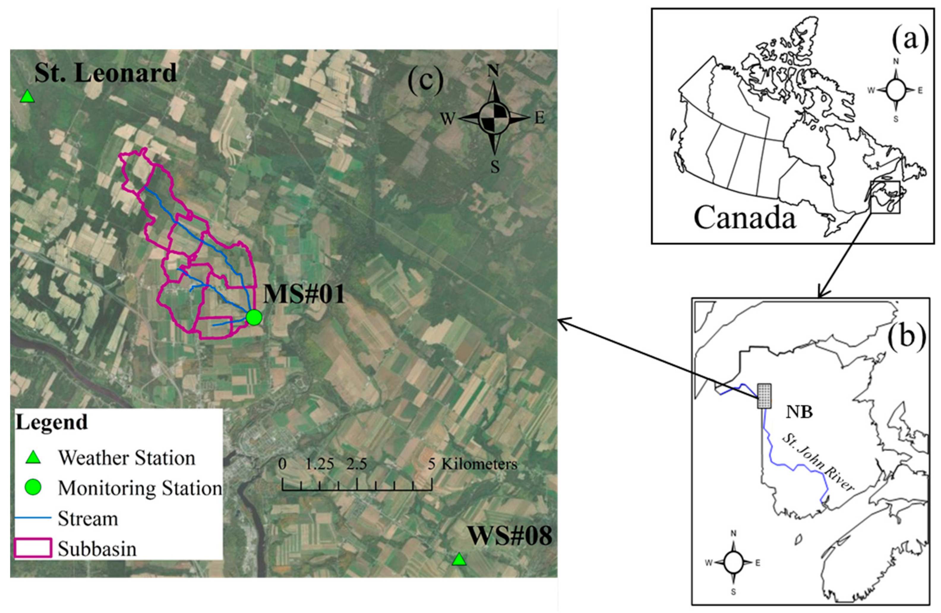
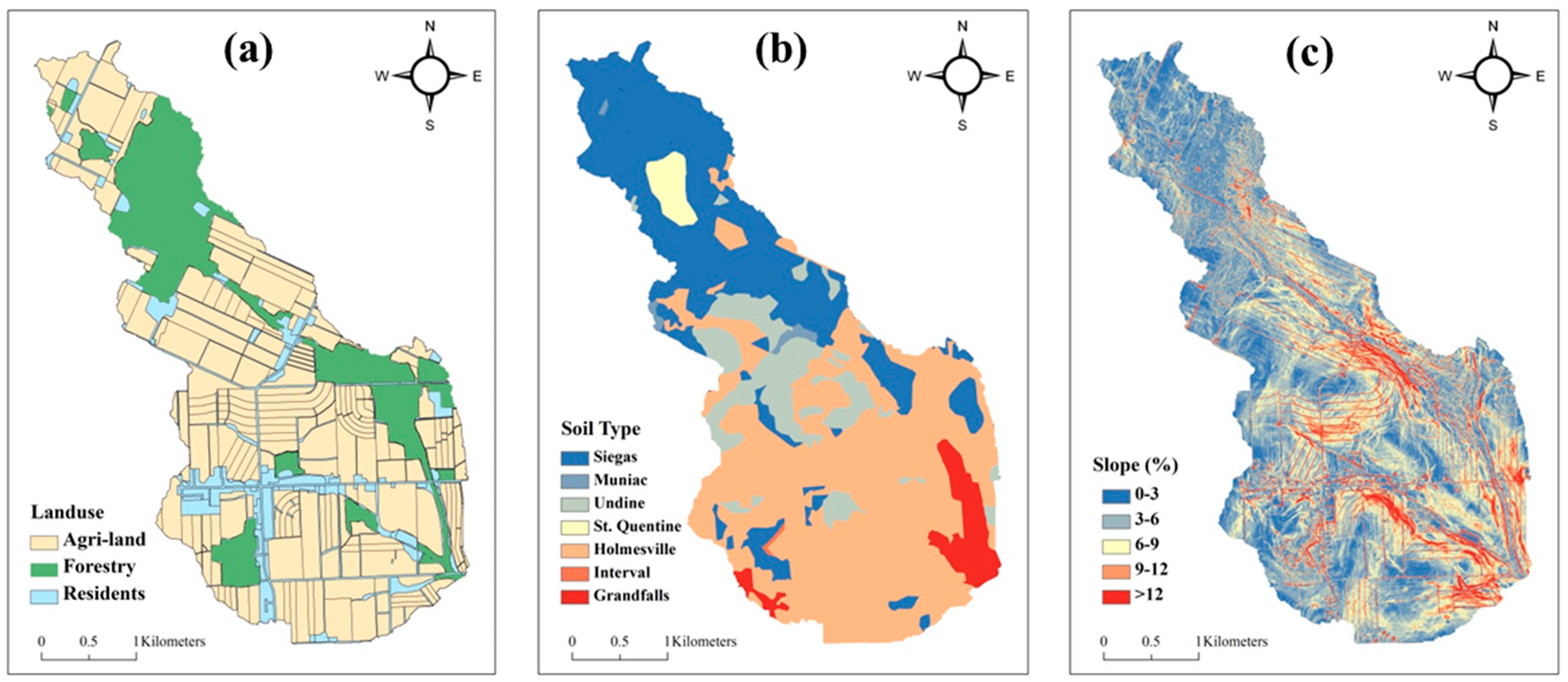
The Black Brook Watershed (BBW), sitting in northwest New Brunswick, Canada, is located in the Upper Saint John River Valley ecoregion in the Atlantic Maritime ecozone (Figure 1). This experimental watershed has been studied extensively for more than 20 years, evaluating the impact of agriculture on soil erosion and water quality [25,29]. The watershed covers an area of 14.5 km2, with agricultural land use constituting 65% of the land base of the watershed, with the remainder either forested or used for urban and residential purposes (Figure 2a). Elevations range from 170 to 260 m above mean sea level. Slopes vary from 1% to 6% in the upper basin to 4–9% in the central area. In the lower portion, the slopes are more strongly rolling at 5–16% (Figure 2c). The climate associated with the region is moderately cool boreal with a humid to perhumid moisture regime and with ~120 frost-free days per year, an average daily temperature of 3.7 °C [26], and an annual precipitation amount of 1038 mm [30]. About one-third of the precipitation is snow, and snowmelt leads to major surface runoff and groundwater recharge events from March to May [29]. Although monthly precipitation from April to September is relatively uniformly distributed, frequent summer storm events relocate large amounts of soil within the watersheds. Six mineral soil types, i.e., Grandfalls, Holmesville, Interval, Muniac, Siegas, and Undine, and one organic soil type, St. Quentin, were identified in the BBW by soil surveys (1:10,000 scale; Figure 2b) [31].
At the outlet of the watershed (MS#01; Figure 1), a V-notch weir was installed in 1992, recording the stage height of water with a Campbell Scientific CR10X datalogger. Stage height values were converted to flow rates using a calibration curve function [32]. An ISCO automatic sampler was used to collect water samples (Teledyne ISCO, Lincoln, NE, USA). The sampling frequency was set at one sample every 72 h during the base flow period. During runoff events, the sampling frequency increased to one sample every 5-cm change in stage height. The samples were analyzed for concentrations of suspended solids, nitrate-nitrogen (NO3-N), and soluble-phosphorus (Sol-P). All of the sample analyses were conducted in the Soil and Hydrology Laboratory in the Fredericton Research and Development Centre. In brief, after measuring the volume, each sample was first filtered through a 0.45 μm (0.000018 in) semipermeable membrane (Millipore Corp., Billerica, MA, USA) to determine the suspended solids concentration. The remaining filtrate was measured for pH and conductivity and then was analyzed for pollutant concentrations using a Flow Injection Analyzer [32]. The monthly loadings were determined by integrating discrete loadings, which were calculated by suspended solid/nutrient concentration × stream discharge for each sampling period.
The climate data, including daily precipitation, air temperature, relative humidity, and wind speed, were obtained from the St. Leonard Environment Canada weather station, located approximately 5 km from the BBW (Figure 1). The daily average relative humidity and wind speed were calculated based on hourly values. Since this weather station did not monitor daily solar radiation, this study used solar radiation collected from a weather station located approximately 10 km from the BBW (WS#08; Figure 1).
Since the early 1990s, a land use survey has been conducted every year in the BBW to record land use and management practices, including crop types, tillage operations, and fertilizer and pesticide applications on each farmland. During the past few decades, potato-barley crop rotation has been the dominant agricultural practice. Major BMPs are flow diversion terraces (FDT) and associated grassed waterways, protecting more than half of the agricultural area in 2011. In particular, a land use map was generated annually from 1992 to 2011 based on land use surveys, recording detailed information about field IDs, land transactions, crop rotation, and detailed management practices (e.g., names of fertilizers, composition, and application amounts and dates).
2.2. SWAT Setup
The basic input data included the DEM, land use, and soil maps for the BBW. A high-resolution light detection and ranging (LiDAR) based DEM (1-m resolution) was used to delineate the watershed and derive topographical characteristics [33,34]. The land use types in BBW are surveyed each year by Agriculture and Agri-Food Canada (AAFC) and summarized in Table 1. The soil data were obtained from an AAFC detailed soil survey map [31]. ArcSWAT 2012 was used to delineate the boundaries of the entire study area and its subbasins, along with their drainage channels. The BBW was divided into eight subbasins corresponding to surveys by AAFC. The areas of the individual subbasins ranged from 68 to 278 ha in size. Table 2 lists the characteristics of generated subbasins and stream attributes of subbasins. Slopes in the BBW were classified into five groups (Figure 2).
2.2.1. New Land Use Map
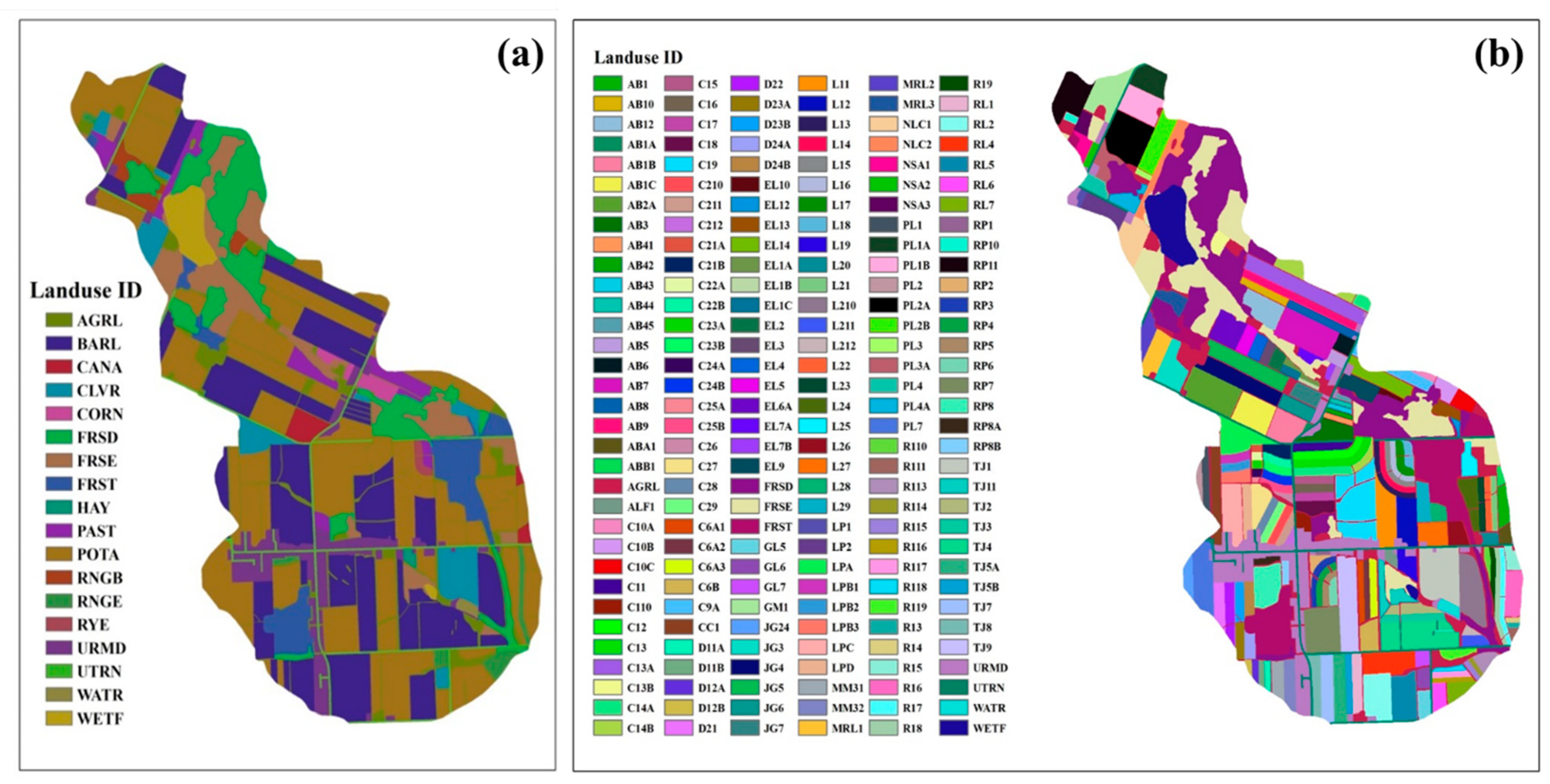
Two versions of the enhanced SWAT model were set up for the BBW, using detailed and coarse inputs of land use and management practices, referred to as SWAT1 and SWAT2, respectively, hereafter. The conventional way of setting up SWAT uses one land use map with the crop name as the land use ID. When HRUs are created with specified combinations of land use type, soil type, and slopes in a subbasin, one HRU can represent multiple fields. This study assigned a unique land use ID (based on farmers’ names and field numbers) to each field identified in the land use map. If two fields had the same crop present, e.g., potatoes, they were assigned different land use IDs. The land use map of 2001 was chosen as the baseline map to delineate HRUs for SWAT1 and SWAT2. Figure 3a shows the land use map used for SWAT2 with 18 land use IDs. By contrast, 198 land use IDs were identified in the new land use map used for SWAT1 (Figure 3b). After combining the land use, soil, and slope maps (with area thresholds of 0, 10, and 20%, respectively) through the ArcSWAT interface, 887 and 310 HRUs were created for SWAT1 and SWAT2, respectively (Table 2).
2.2.2. Management Data Configuration
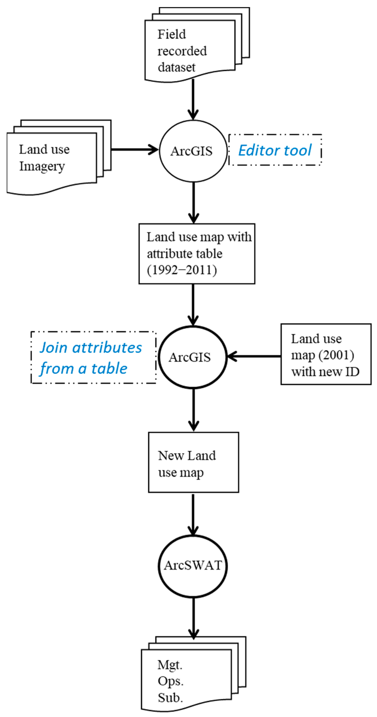
To incorporate the recorded data into the SWAT1 management files, land use maps from 1992 to 2011 (except for 2001) were spatially joined with the new land use map based on field IDs (Figure 3b) through ArcGIS (join attributes from a table; Figure 4). As a result, the new land use map had an attribute table with 20 years of land use and management information associated with each field. The parameters of the SWAT1 management files (based on HRUs) were further modified according to field records. For example, a moldboard plow with a 150-mm mixing depth and 0.95 mixing efficiency was set for conventional tillage, and a chisel plow with a 150-mm mixing depth and 0.30 mixing efficiency was set for conservation tillage. Existing terracing and grassed waterways modules were modified corresponding to records, including the year of implementation, slope lengths of FDT, and widths of grassed waterways. The parameters of these BMPs were initially modified according to published values [35,36,37,38,39].
We assumed that only one land use map (2001) was available for SWAT2, and limited land use and management information was used to adjust SWAT2 management files (Table 1). As a result, the following assumptions based on the information available were made:
- (1)
- Potato–barley was assigned to land use ID POTA. For other land use IDs, it was assumed that no crop rotation took place;
- (2)
- Fertilizers were applied only to potato and barley, and fertilizer amounts and N/P ratios were averaged over the entire watershed based on 2001 survey data from the BBW;
- (3)
- Contour tillage was applied only to potato and barley fields, and tillage areas were proportionally assigned to potato and barley fields over the entire watershed based on 2001 survey data from the BBW; and
- (4)
- FDT and grassed waterways were applied only to potato and barley fields, and their areas were proportionally assigned to potato and barley fields in individual subbasins based on 2001 survey data from the BBW.
2.3. SWAT Calibration and Validation
The SWAT calibration uncertainty program (SWAT-CUP) was used to calibrate both models [40]. Water quantity and quality in the SWAT model were calibrated sequentially. SWAT1 was first calibrated using monthly baseflows, then the total stream discharges from 1992 to 2001. The baseflow discharge was based on previously reported values calculated using the recursive digital filter (RDF) method [41,42]. Further calibration was conducted first to monthly sediment, second to NO3-N, and last to Sol-P loadings from 1992 to 2001. During calibration, we tried to avoid the equifinality problem and the best-fit of parameter sets by using thousands of simulations aided with SWAT-CUP for each water quantity and quality variable. The validation period was from 2002 to 2011. Parameters TERR_P and TERR_CN of the terracing module and USLE_P for the impact of contour tillage on sediment loading were also calibrated (Table 3). As for SWAT2, calibration parameters were set equal to those for SWAT1 with respect to water flow and sediment and nutrient loadings, as well as management practices (i.e., contour tillage, FDT, and grassed waterways). The model’s performance in simulating water quantity and quality at the watershed outlet was compared between SWAT1 and SWAT2 based on two periods, i.e., period Ι (1992–2001) and period ΙΙ (2002–2011).
2.4. Statistical Evaluation
Statistical metrics used to evaluate model performance include the relative error (Re), the coefficient of determination (R2), and the Nash–Sutcliffe (NS) coefficient [43], expressed as follows:
where Oi and Pi are the observed and predicted values, respectively, and Oavg and Pavg are the averages of the observed and predicted values, respectively.
3. Results and Discussion
3.1. Input Resolutions of Land Use and Management Practices
3.1.1. Crop Rotation, Fertilizer Application, and Contour Tillage
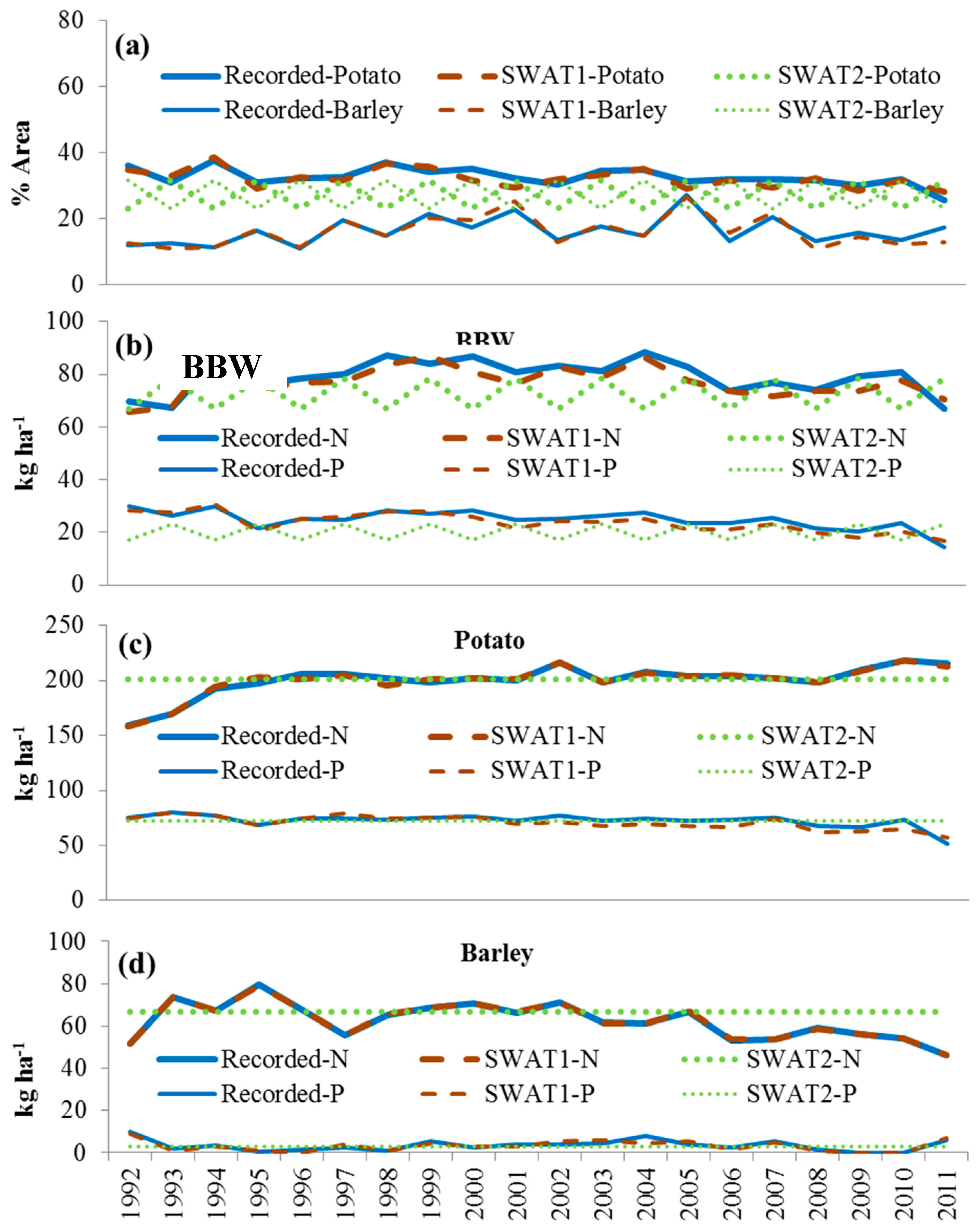
Percentage areas of potato and barley and annual application rates of N and P for BBW, represented with both models, were compared with records from 1992 to 2011 (Figure 5). For SWAT1, input areas for the two crops were consistent with records, with potatoes occupying 30 to 40% of the total watershed area and barley areas varying from 10 to 25%, with high percentages in the early 2000s (Figure 5a). Application rates of N for potato fields were almost constant after 1995 at ~200 kg ha−1, but decreased from ~60 kg ha−1 in the 1990s to less than 50 kg ha−1 in the late 2000s for barley fields (Figure 5c,d). The application rates of P for potato and barley fields were relatively constant at ~70 kg ha−1 and 5 kg ha−1, respectively (Figure 5c,d). Overall, the input N and P application rates of SWAT1 agreed well with field records for both potato and barley fields. For SWAT2, input areas of potato and barley and N and P application rates did not agree well with the field records (Figure 5). The input areas of potato and barley in 2001 were consistent with records, while in other years, they varied up and down due to potato-barley rotations. Input fertilizer application rates in potato and barley fields in 2001 were consistent with records, remaining constant for other years. For the entire watershed, N and P application rates varied with potato–barley rotations (Figure 5).
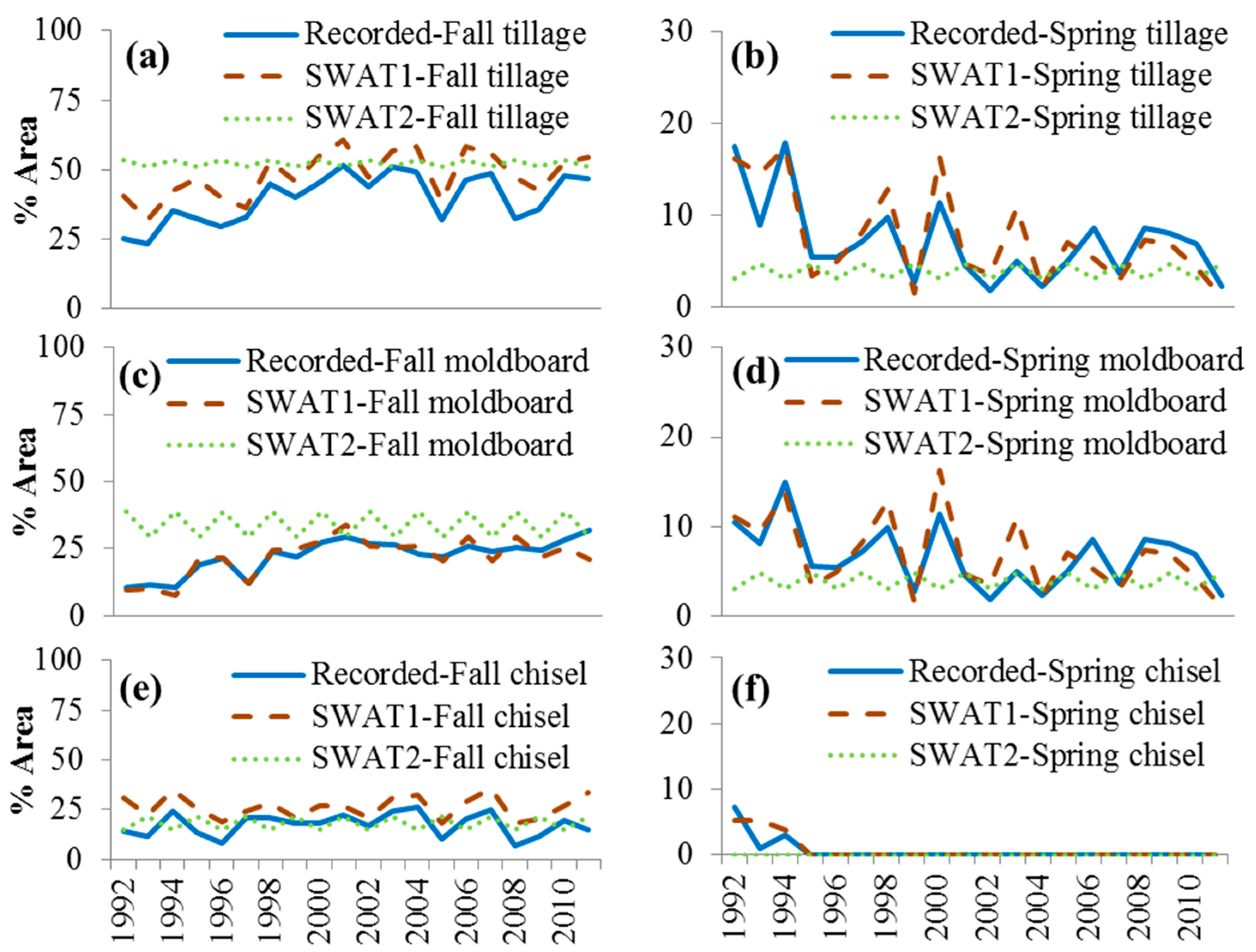
Figure 6 shows the input percentage areas of various tillage operations in the BBW compared with records from 1992 to 2011. For SWAT1, input areas of moldboard and chisel plow, as well as total tillage areas, were consistent with records in both spring and fall (Figure 6c–f). The chisel plow areas were slightly higher than records (about 5% higher), leading to an overestimation of the total tillage area in fall (Figure 6a,e). This was caused by the modifications we made to the contour tillage operation for several crops. Although spring tillage areas decreased and fall tillage increased from 1992 to 2011, fall tillage areas were always much greater than spring tillage areas (Figure 6a,b). In addition, fall moldboard plow areas increased in the 1990s and remained constant in the 2000s, occupying ~25% of the total watershed area (Figure 6c). Fall chisel plow areas remained under 25% of the total watershed area, with several peaks in the early 2000s (Figure 6e). Spring moldboard plow areas have decreased since the early 1990s, and spring chisel plow areas decreased to 0% after 1995 (Figure 6d,f). For SWAT2, input areas for moldboard and chisel plowing were not consistent with records (Figure 6). The percentage areas for contour tillage were equal to the records only in 2001, while in other years, they varied with potato–barley rotations.
3.1.2. Terraces and Grassed Waterways
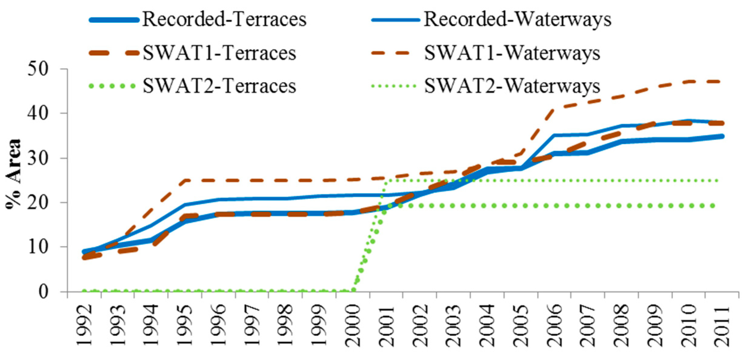
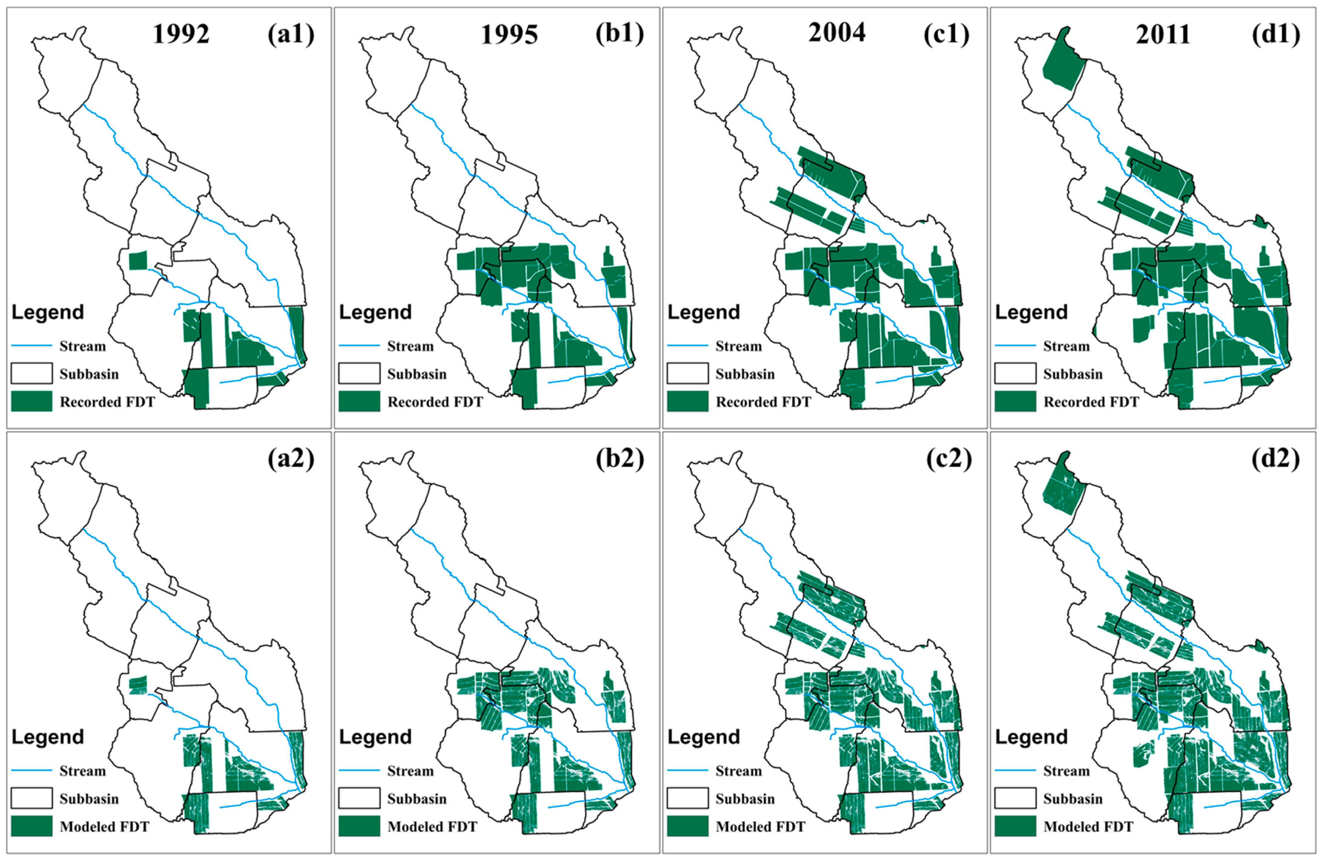
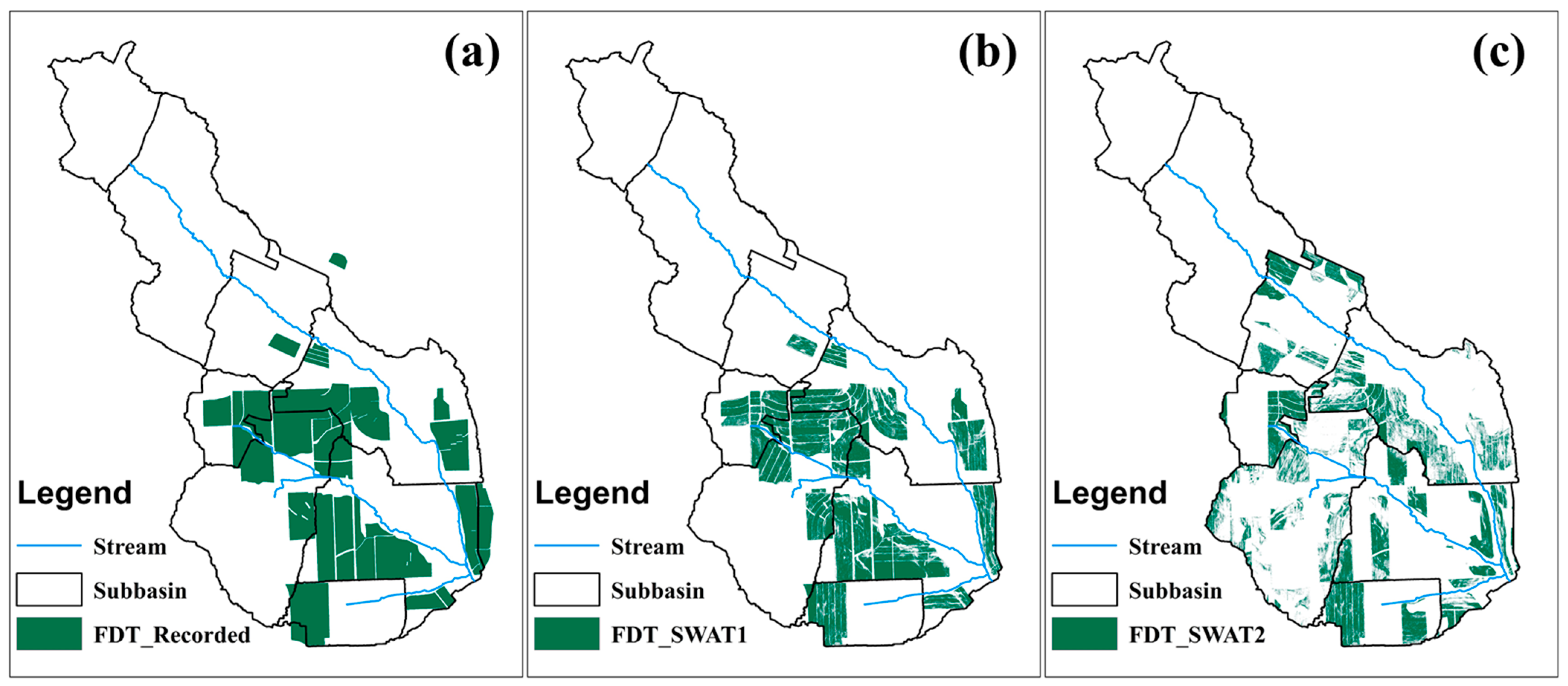
The input percentage areas of FDT and grassed waterways were compared with records from 1992 to 2011 (Figure 7). Since most grassed waterways were constructed along with FDT, input terraces and waterways varied similarly over time. The total areas protected by FDT and grassed waterways increased from less than 10% to almost 40% from 1992 to 2011. For SWAT1, input FDT protected areas were consistent with records, and input grassed waterway protected areas were slightly greater than records, caused by missing data in several fields. Comparisons between input FDT protected areas and records in 1992, 1995, 2004, and 2011 for SWAT1 (Figure 8) show that SWAT1 successfully represented changes in FDT protected areas from 1992 to 2011. Input FDT and grassed waterway protected areas for SWAT2 were close to records only in 2001, remaining constant after 2001 (Figure 7). Although SWAT2 could generate equal areas with records for most subbasins, it could not generate the same FDT distribution pattern as SWAT1 (Figure 9).
3.2. SWAT Calibration
Table 4 lists the calibrated parameters for SWAT1, where 20 parameters were adjusted. Parameter CNOP (i.e., CN2) was initially adjusted to reflect the influences of management practices based on land use groups and hydrological properties of soils. Alpha_Bf was adjusted to 0.04 day−1, indicating that the baseflow discharge had a slow response to recharge. The parameter Surlag was set to 0.075, indicating that surface runoff tended to converge quickly to the outlet. We also adjusted the relevant parameters to reflect that lateral flow increased due to unfrozen soils in winter [44]. Additionally, parameter Anion_Excl was reduced to improve the nitrate retention capacity of soils. Table 3 lists parameters calibrated for management practices. Support practice factor (parameter ULSE_P) values for contour tillage and FDT were within the range of recommended values [35,37,38]. The value of parameter TERR_CN (i.e., 72) was less than the mean CN2 of croplands without FDT. Note that TERR_SL for SWAT2 was set to 50 m, while for SWAT1, the value varied in different HRUs, ranging from 25 to 100 m.
3.3. Impacts on Monthly Water Flow and Sediment and Nutrient Loadings
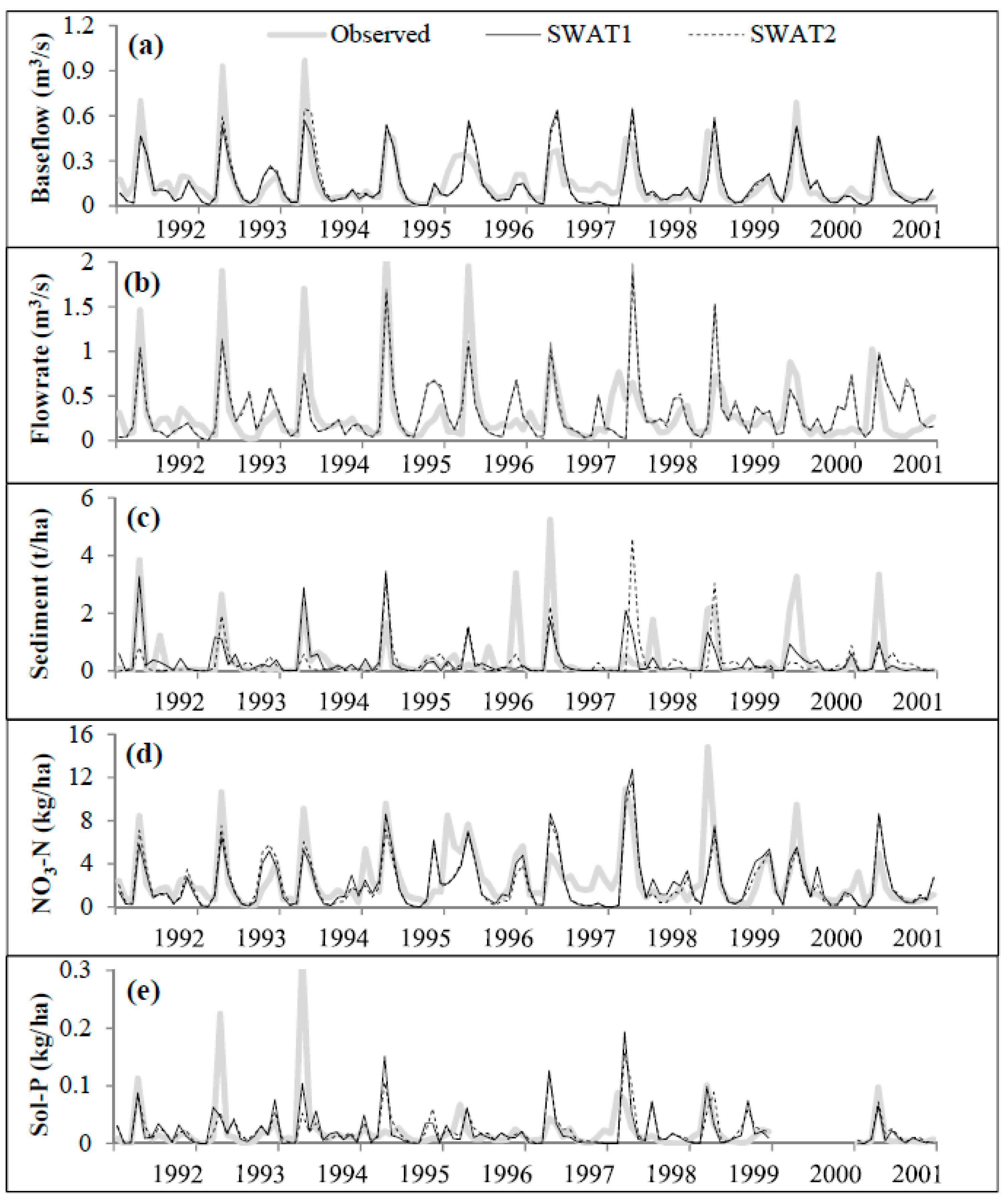
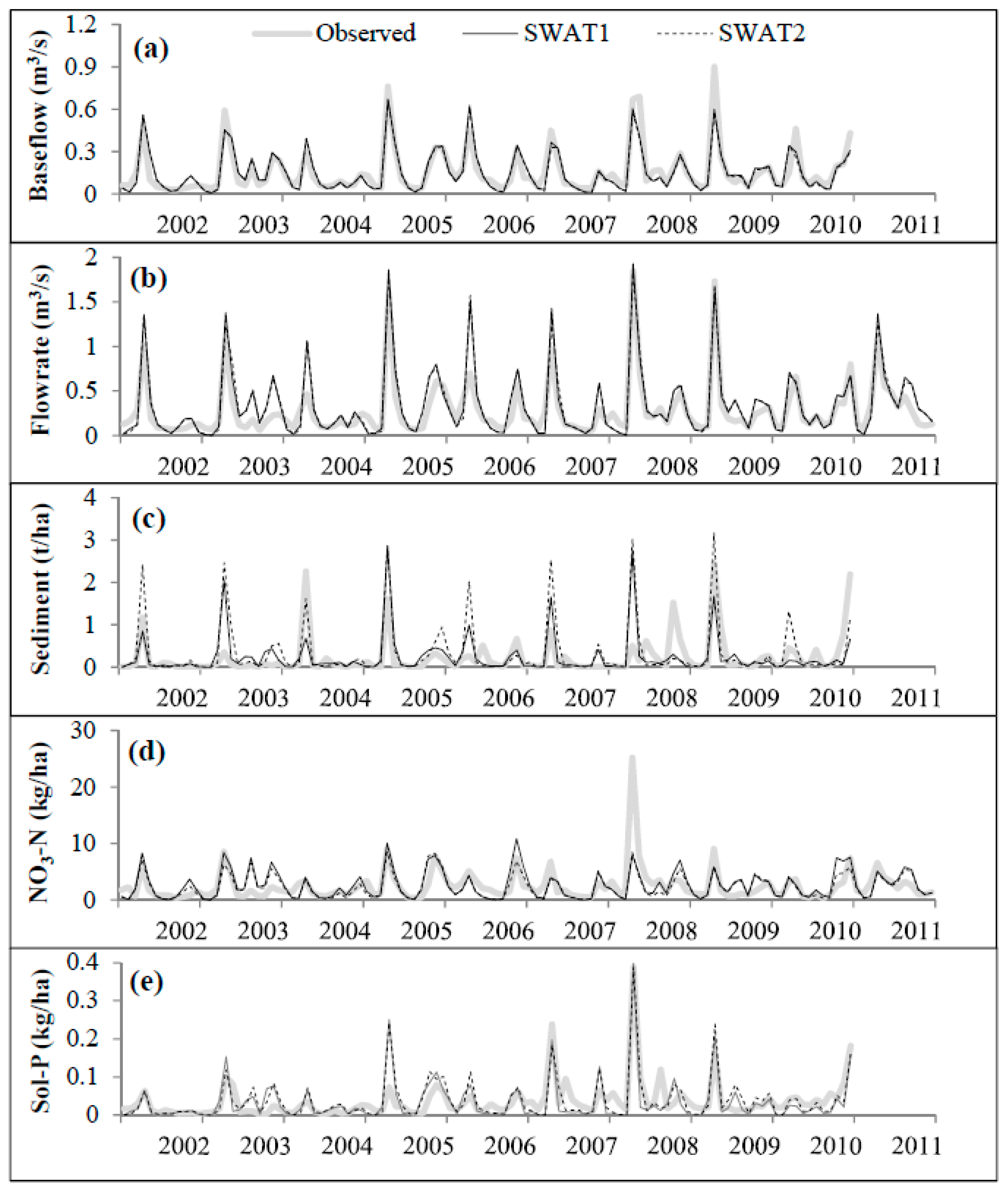
Figure 10 and Figure 11 show simulated and observed monthly water flows and sediment and nutrient loadings for periods Ι and ΙΙ, respectively. Table 5 lists statistical indexes for model performances.
The monthly baseflow and total stream discharge simulated by both models were consistent with observations (or estimates of baseflow) in both periods (Figure 10a,b and Figure 11a,b, respectively). Both models performed satisfactorily according to guidelines established by Moriasi et al. [45]. Compared with SWAT2, SWAT1 performed slightly better in simulating monthly variations of total stream discharge for both periods and the baseflow for period ΙΙ (i.e., greater R2 and NS), while in period Ι, SWAT2 performed slightly better (Table 5). In both periods, the Re of SWAT1 was close to that of SWAT2 for baseflow and total stream discharge (Table 5). The results indicate that discrepancies in the management practice input between these two models had little impact on the general water balance in the BBW.
The two models performed almost equivalently in simulating the monthly variations of sediment loading in period Ι based on R2 and NS (Table 5). However, visual inspection indicates that SWAT1 accurately identified several major peaks of sediment loading during the snowmelt season (e.g., 1992 and 1994), whereas SWAT2 severely underestimated them (Figure 10c). In general, both models underestimated sediment loadings in period Ι (Re = −20.3 and −16.1 for SWAT1 and SWAT2, respectively) due to a failure to capture major erosion events caused by snowmelt in humid-warm winters (e.g., 1996 to 2000; Figure 10c). In period ΙΙ, SWAT1 performed better than SWAT2 (i.e., greater NS; Table 5), with the latter consistently overestimating peak sediment loadings during the snowmelt season (Re = 35.9; Figure 11). This is because SWAT1 was able to better account for gradually increasing areas of FDT after 2001 (Figure 7 and Figure 8). However, the low NS values of both models in period ΙΙ were partly due to the inability of the SWAT model’s modified universal soil loss equation to address soil erosion caused by freeze–thaw cycles. The FDT module could not be calibrated to compensate for incorrect estimates of sediment loadings. An accurate soil erosion module is required for a better assessment of FDT during winter and the snowmelt season in Atlantic Canada.
SWAT2 performed slightly better than SWAT1 in simulating monthly variations of NO3-N loading for both periods (i.e., higher R2 and NS; Table 5). Both models tended to underestimate monthly NO3-N loading in period I (negative Re values), while SWAT1 overestimated NO3-N loading in period II. Since SWAT1 can model gradually increased FDT protected areas (Figure 7), it was expected that more nitrates would be leached due to increased infiltration, which is reflected by the change of sign of Re for SWAT1 from period I to II.
For Sol-P loading, SWAT1 performed better in simulating monthly variations than SWAT2 in period Ι (i.e., higher R2 and NS) while not as well in period ΙΙ (i.e., lower R2 and NS; Table 5). Note that for both models, NS and R2 values for Sol-P in period I were lower than those in period II, mainly due to several snowmelt peaks in the early 1990s (e.g., 1993 and 1994), which both models failed to simulate, consistent with the issue simulating stream discharge for the same periods (Figure 10b versus e). This illustrates that even though statistical indices indicate that stream discharge was reasonably simulated, the discrepancy between simulations and observations can be amplified in associated nutrients, particularly for extreme high-flow events. This is one of the SWAT limitations in simulations at daily or event scales [46]. Furthermore, changing the sign of Re from positive (overestimation) to negative (underestimation) from period I to II with SWAT1 indicates less Sol-P loadings as a response to the gradually increased area protected by FDT, leading to increased infiltration and decreased surface runoff (Table 5).
Overall, there is no definite increase in simulation accuracy in monthly variations of nutrient loadings with high spatial and temporal resolution management input data in our study, though monthly nutrient loading simulations were sensitive to management configuration.
3.4. Impacts on Annual Stream Flow and Sediment and Nutrient Loadings
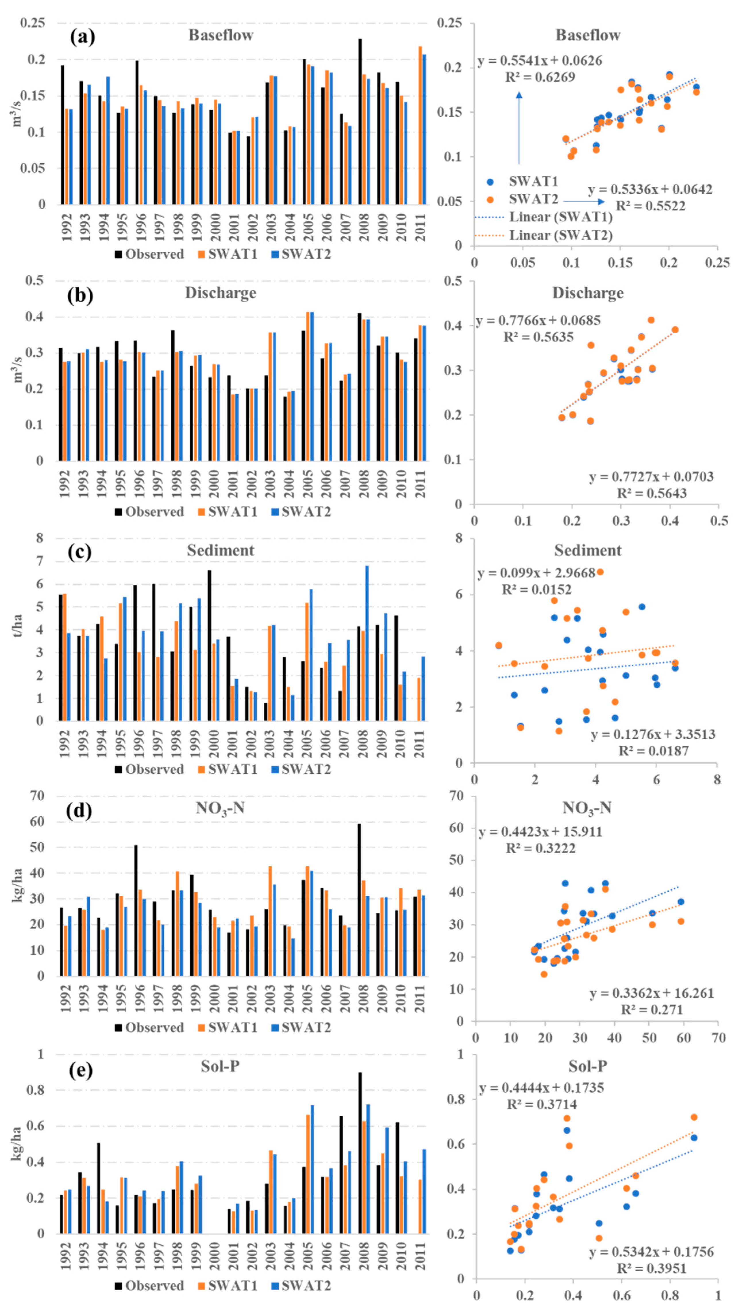
Figure 12 shows observed and simulated annual baseflow and total discharge and sediment, NO3-N and Sol-P loadings by SWAT1 and SWAT2 from 1992 to 2011. SWAT1 simulated baseflow better than SWAT2 (i.e., R2 = 0.63 > R2 = 0.55), and both models performed similarly with total discharge (R2 = 0.56; Figure 12a,b), indicating again that there are discrepancies in the land use and management practice input between these two models had minimum impact on the general water balance in the BBW. Both models simulated annual sediment loadings poorly (i.e., R2 ≤ 0.02; Figure 12c) due to the inability of the SWAT model to address soil erosion caused by freeze–thaw cycles, which rendered difficulties in the assessment of FDT input accuracy effects on simulation. Compared with monthly evaluation (Figure 10 and Figure 11), the annual variations in sediment loading were poorly simulated (based on R2), demonstrating that monthly calibration would not guarantee good annual results. This is particularly evident for sediment loading, whose one or two peaks control the majority of monthly variations over a year. SWAT1 performed better than SWAT2 on simulating variations of annual loading for NO3-N (i.e., R2 = 0.32 > R2 = 0.27) while SWAT2 was better for Sol-P based on R2 (i.e., R2 = 0.40 > R2 = 0.37; Figure 12d,e). Similar to the monthly evaluation, there is no definite increase in simulation accuracy in annual variations of stream flow and nutrient loadings with high spatial and temporal management inputs in our study.
3.5. Spatial Impact of FDT on Soil Erosion
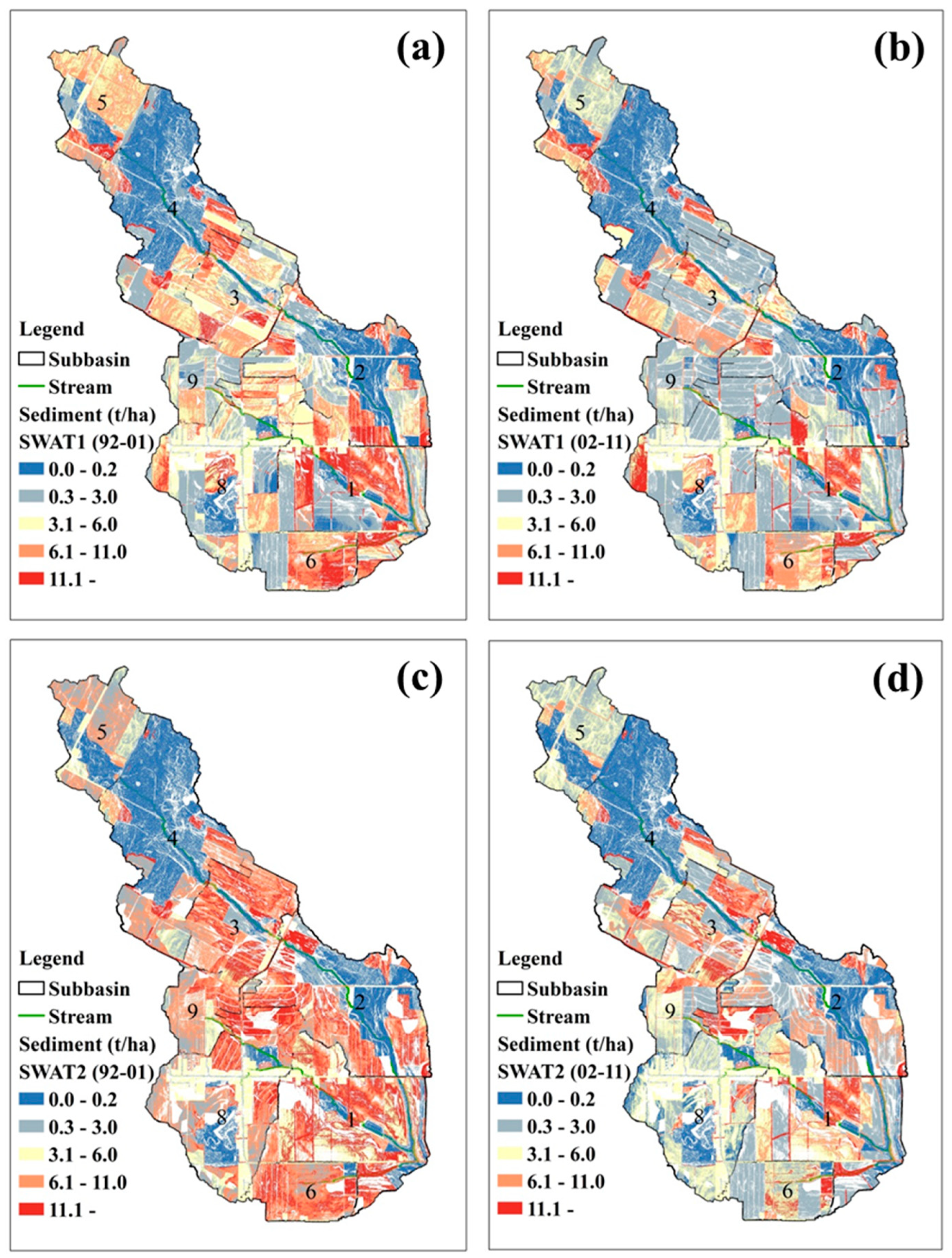
SWAT1- and SWAT2-simulated annual sediment loadings from HRUs were averaged over periods Ι and ΙΙ, and erosion intensity maps were derived (Figure 13). The sediment loadings were classified into five groups according to Lobb et al. [47]. Soil loss rates greater than 11 t ha−1 were considered a moderate to high erosion intensity, and soil loss rates less than 11 t ha−1 were considered a low erosion intensity. Simulated moderate to high-intensity erosion areas decreased from period Ι to ΙΙ for both models (Figure 13), corresponding to the increased usage of FDT in period ΙΙ (Figure 7). For SWAT1, most low erosion intensity areas were associated with FDT in both periods (Figure 8 and Figure 13), except for forested land (Figure 2). By contrast, low erosion intensity areas modeled with SWAT2 were not consistent with the actual FDT distribution in the BBW for both periods (Figure 8 and Figure 13). SWAT2 failed to spatially represent the impact of FDT on soil erosion across the watershed. These results indicate that SWAT can provide high-resolution output, such as soil-erosion-vulnerable areas, using high-resolution management inputs through field-based HRU delineation. SWAT can thus better facilitate decision-making not only at the subbasin scale but also at the field scale.
4. Comparing with Other Studies
To our knowledge, there is no study for dynamic land use impacts having land use and management information for every year of the simulation period. Particularly, no study has such detailed management practice records for each simulation year as in our study. Furthermore, previous studies investigating the difference between static and dynamic land use and management practice inputs used the earliest land use map available as the static condition and baseline scenario. As a result, they found obvious effects of land use changes on the simulation of flow, and sediment, nitrogen, and phosphorus loadings [48,49,50,51] and argued that differences in the land use input conditions could affect the long-term water quantity and quality simulation so that dynamic land use input was recommended. On the contrary, we used the land use map of 2001 (in the middle of the simulation period from 1992 to 2011) and limited management information as the static land use and management practice input for SWAT2. As a result, we obtained a different conclusion that there is no definite increase in simulation accuracy in monthly and annual water flow and nutrient loadings with high spatial and temporal resolution management input data in our study. This is because land use and management information from 2001 (though we have tried to simplify inputs such as N and P application and crop rotation) could be seen as an average management condition of BBW from 1992 to 2011. In addition, the area of agricultural lands and management practices used in the BBW (except for the area of FDT) did not change too much over the simulation period. Our results indicate that SWAT, although set up with limited land use and management information, is able to provide comparable simulations of water quantity and quality at the watershed outlet, as long as the estimated land use and management practice data can reasonably represent the average land use and management condition of the watershed over the target simulation period. However, the conclusion may not be applicable to watersheds with great changes in the area of agricultural lands and management practices during the simulation period.
5. Conclusions
This study presents an algorithm that incorporates detailed land use and management inputs into the SWAT model. The method delineates HRUs based on field boundaries and associates each HRU with an individual field to facilitate incorporating detailed annual records into the SWAT management files. After model setup, the SWAT model was calibrated and validated using monthly water flow and sediment and nutrient loadings in a small experimental watershed in New Brunswick, Canada. Meanwhile, another SWAT model was set up with the original HRU-delineation method and limited information on land use and management. These two versions of SWAT were compared with respect to input and output resolution and prediction accuracy of monthly and annual water flow and sediment and nutrient (NO3-N and Sol-P) loadings. Compared with the SWAT set up with the conventional method, the SWAT set up with the new method generated accurate annual areas of crops, fertilizer application, tillage operation, flow diversion terraces (FDT), and grassed waterways in the BBW. The simulation results indicate that the SWAT set up with the new method did not evidently perform better than the SWAT set up with the conventional method in simulating monthly variations of stream discharge and NO3-N and Sol-P loadings, though monthly nutrient loading simulations were sensitive to management configuration.; however, it did improve the simulation of monthly sediment loading due to an improved representation of FDT in the watershed, and it was able to estimate the spatial impact of FDT on soil erosion across the entire watershed. Setting up SWAT with detailed land use and management information using the field-based HRU-delineation method could specify sources of pollutants and vulnerable areas in subbasins, facilitating watershed management decision-making. Furthermore, the annual examination also showed comparable simulation accuracy on water flow and nutrient loadings between the two models. We concluded that there was no definite increase in simulation accuracy in water flow and nutrient loadings with high spatial and temporal management inputs, indicating that SWAT, although set up with limited land use and management information, is able to provide comparable simulations of water quantity and quality at the watershed outlet, as long as the estimated land use and management practice data can reasonably represent the average land use and management condition of the watershed over the target simulation period.
Author Contributions
Conceptualization, J.Q.; methodology, J.Q.; software, J.Q.; validation, F.M. and S.L.; formal analysis, J.Q.; investigation, J.Q.; resources, S.L.; data curation, X.K. and S.L.; writing—original draft preparation, J.Q.; writing—review and editing, J.Q. and X.K.; visualization, X.K.; supervision, F.M. and S.L.; project administration, F.M. and S.L.; funding acquisition, F.M. and S.L. All authors have read and agreed to the published version of the manuscript.
Funding
The funding support for this project was provided by Agriculture and Agri-Food Canada (AAFC) through project #1145, entitled “Integrating selected BMPs to maximize environmental and economic benefits at the field and watershed scales for sustainable potato production in New Brunswick” and the Natural Science and Engineering Research Council (NSERC) through Discovery Grants to FRM. The authors are thankful to S. Lavoie, J. Monteith, and L. Stevens for their technical support in data collection and sample analyses.
Institutional Review Board Statement
Not applicable.
Informed Consent Statement
Not applicable.
Data Availability Statement
The data presented in this study are available on request from the corresponding author.
Conflicts of Interest
The authors declare no conflict of interest.
References
- Singh, V.P.; Frevert, D.K. Watershed Models; CRC Press: Boca Raton, FL, USA, 2005. [Google Scholar]
- Junyu, Q.; Liying, S.; Qiangguo, C. Zonal differences of runoff and sediment reduction effects for typical management small watersheds in China. Int. Soil Water Conserv. Res. 2013, 1, 39–48. [Google Scholar] [CrossRef] [Green Version]
- Sharpley, A.N.; Williams, J.R. EPIC-Erosion/Productivity Impact Calculator: 1. Model Documentation; Technical Bulletin-United States Department of Agriculture: Washington, DC, USA, 1990. [Google Scholar]
- Laflen, J.M.; Lane, L.J.; Foster, G.R. WEPP: A new generation of erosion prediction technology. J. Soil Water Conserv. 1991, 46, 34–38. [Google Scholar]
- Graham, D.N.; Butts, M.B. Flexible, integrated watershed modelling with MIKE SHE. Watershed Models 2005, 849336090, 245–272. [Google Scholar]
- Beasley, D.; Huggins, L.; Monke, A. ANSWERS: A model for watershed planning. Trans. ASAE 1980, 23, 938–944. [Google Scholar] [CrossRef]
- Young, R.A.; Onstad, C.; Bosch, D.; Anderson, W. AGNPS: A nonpoint-source pollution model for evaluating agricultural watersheds. J. Soil Water Conser. 1989, 44, 168–173. [Google Scholar]
- Hundecha, Y.; Bárdossy, A. Modeling of the effect of land use changes on the runoff generation of a river basin through parameter regionalization of a watershed model. J. Hydrol. 2004, 292, 281–295. [Google Scholar] [CrossRef]
- Manguerra, H.; Engel, B. Hydrological Parameterization of Watersheds for Runoff Prediction Using SWAT. JAWRA J. Am. Water Resour. Assoc. 1998, 34, 1149–1162. [Google Scholar] [CrossRef]
- Beven, K. Changing ideas in hydrology—The case of physically-based models. J. Hydrol. 1989, 105, 157–172. [Google Scholar] [CrossRef]
- Goulden, T.; Jamieson, R.; Hopkinson, C.; Sterling, S.; Sinclair, A.; Hebb, D. Sensitivity of hydrological outputs from SWAT to DEM spatial resolution. Photogramm. Eng. Remote Sens. 2014, 80, 639–652. [Google Scholar] [CrossRef]
- Kalcic, M.M.; Chaubey, I.; Frankenberger, J. Defining Soil and Water Assessment Tool (SWAT) hydrologic response units (HRUs) by field boundaries. Int. J. Agric. Biol. Eng. 2015, 8, 69–80. [Google Scholar]
- Ahiablame, L.; Sinha, T.; Paul, M.; Ji, J.-H.; Rajib, A. Streamflow response to potential land use and climate changes in the James River watershed, Upper Midwest United States. J. Hydrol. Reg. Stud. 2017, 14, 150–166. [Google Scholar] [CrossRef]
- Jha, M.; Gassman, P.W.; Secchi, S.; Gu, R.; Arnold, J. Effect of Watershed Subdivision on Swat Flow, Sediment, and Nutrient Predictions. JAWRA J. Am. Water Resour. Assoc. 2004, 40, 811–825. [Google Scholar] [CrossRef] [Green Version]
- Arnold, J.G.; Srinivasan, R.; Muttiah, R.S.; Williams, J.R. Large area hydrologic modeling and assessment part I: Model development. JAWRA J. Am. Water Resour. Assoc. 1998, 34, 73–89. [Google Scholar] [CrossRef]
- Gassman, P.W.; Reyes, M.R.; Green, C.H.; Arnold, J.G. SWAT peer-reviewed literature: A review. In Proceedings of the 3rd International SWAT Conference, Zurich, Switzerland, 11–15 July 2005. [Google Scholar]
- Ullrich, A.; Volk, M. Application of the Soil and Water Assessment Tool (SWAT) to predict the impact of alternative management practices on water quality and quantity. Agric. Water Manag. 2009, 96, 1207–1217. [Google Scholar] [CrossRef]
- Qi, J.; Li, S.; Bourque, C.P.; Xing, Z.; Meng, F.R. Developing a decision support tool for assessing land use change and BMPs in ungauged watersheds based on decision rules provided by SWAT simulation. Hydrol. Earth Syst. Sci. 2018, 22, 3789–3806. [Google Scholar] [CrossRef] [Green Version]
- Qi, J.; Li, S.; Jamieson, R.; Hebb, D.; Xing, Z.; Meng, F.-R. Modifying SWAT with an energy balance module to simulate snowmelt for maritime regions. Environ. Model. Softw. 2017, 93, 146–160. [Google Scholar] [CrossRef]
- Qi, J.; Li, S.; Li, Q.; Xing, Z.; Bourque, C.P.-A.; Meng, F.-R. A new soil-temperature module for SWAT application in regions with seasonal snow cover. J. Hydrol. 2016, 538, 863–877. [Google Scholar] [CrossRef]
- Wang, Q.; Qi, J.; Li, J.; Cole, J.; Waldhoff, S.T.; Zhang, X. Nitrate loading projection is sensitive to freeze-thaw cycle representation. Water Res. 2020, 186, 116355. [Google Scholar] [CrossRef]
- Wang, Q.; Qi, J.; Wu, H.; Zeng, Y.; Shui, W.; Zeng, J.; Zhang, X. Freeze-Thaw cycle representation alters response of watershed hydrology to future climate change. Catena 2020, 195, 104767. [Google Scholar] [CrossRef]
- Abbaspour, K.C.; Rouholahnejad, E.; Vaghefi, S.; Srinivasan, R.; Yang, H.; Kløve, B. A continental-scale hydrology and water quality model for Europe: Calibration and uncertainty of a high-resolution large-scale SWAT model. J. Hydrol. 2015, 524, 733–752. [Google Scholar] [CrossRef] [Green Version]
- Akoko, G.; Le, T.H.; Gomi, T.; Kato, T. A review of SWAT model application in Africa. Water 2021, 13, 1313. [Google Scholar] [CrossRef]
- Li, Q.; Qi, J.; Xing, Z.; Li, S.; Jiang, Y.; Danielescu, S.; Zhu, H.; Wei, X.; Meng, F.-R. An approach for assessing impact of land use and biophysical conditions across landscape on recharge rate and nitrogen loading of groundwater. Agric. Ecosyst. Environ. 2014, 196, 114–124. [Google Scholar] [CrossRef]
- Yang, Q.; Meng, F.-R.; Zhao, Z.; Chow, T.L.; Benoy, G.; Rees, H.W.; Bourque, C.P.-A. Assessing the impacts of flow diversion terraces on stream water and sediment yields at a watershed level using SWAT model. Agric. Ecosyst. Environ. 2009, 132, 23–31. [Google Scholar] [CrossRef]
- Gassman, P.W.; Reyes, M.R.; Green, C.H.; Arnold, J.G. The soil and water assessment tool: Historical development, applications, and future research directions. Trans. ASABE 2007, 50, 1211–1250. [Google Scholar] [CrossRef] [Green Version]
- Ning, J.; Gao, Z.; Lu, Q. Runoff simulation using a modified SWAT model with spatially continuous HRUs. Environ. Earth Sci. 2015, 74, 5895–5905. [Google Scholar] [CrossRef]
- Chow, T.; Rees, H. Impacts of Intensive Potato Production on Water Yield and Sediment Load (Black Brook Experimental Watershed: 1992–2002 Summary); Potato Research Centre, AAFC: Fredericton, NB, Canada, 2006; p. 26. [Google Scholar]
- Zhao, Z.; Chow, T.L.; Yang, Q.; Rees, H.W.; Benoy, G.; Xing, Z.; Meng, F.-R. Model prediction of soil drainage classes based on digital elevation model parameters and soil attributes from coarse resolution soil maps. Can. J. Soil Sci. 2008, 88, 787–799. [Google Scholar] [CrossRef]
- Mellerowicz, K.T. Soils of the Black Brook Watershed St. Andre Parish, Madawaska County; New Brunswick Department of Agriculture: Fredericton, NB, Canada, 1993. [Google Scholar]
- Chow, L.; Xing, Z.; Benoy, G.; Rees, H.; Meng, F.; Jiang, Y.; Daigle, J. Hydrology and water quality across gradients of agricultural intensity in the Little River watershed area, New Brunswick, Canada. J. Soil Water Conserv. 2011, 66, 71–84. [Google Scholar] [CrossRef] [Green Version]
- Zhao, Z.; Benoy, G.; Chow, T.L.; Rees, H.W.; Daigle, J.-L.; Meng, F.-R. Impacts of accuracy and resolution of conventional and LiDAR based DEMs on parameters used in hydrologic modeling. Water Resour. Manag. 2010, 24, 1363–1380. [Google Scholar] [CrossRef]
- Qi, J.; Liang, K.; Li, S.; Wang, L.; Meng, F.-R. Hydrological evaluation of flow diversion terraces using downhill-slope calculation method for high resolution and accuracy DEMs. Sustainability 2018, 10, 2414. [Google Scholar] [CrossRef] [Green Version]
- Yang, Q.; Zhao, Z.; Chow, T.L.; Rees, H.W.; Bourque, C.P.A.; Meng, F.R. Using GIS and a digital elevation model to assess the effectiveness of variable grade flow diversion terraces in reducing soil erosion in northwestern New Brunswick, Canada. Hydrol. Process. 2009, 23, 3271–3280. [Google Scholar] [CrossRef]
- Yang, Q.; Zhao, Z.; Benoy, G.; Chow, T.L.; Rees, H.W.; Bourque, C.P.-A.; Meng, F.-R. A watershed-scale assessment of cost-effectiveness of sediment abatement with flow diversion terraces. J. Environ. Qual. 2010, 39, 220–227. [Google Scholar] [CrossRef] [PubMed]
- Haan, C.T.; Barfield, B.J.; Hayes, J.C. Design Hydrology and Sedimentology for Small Catchments; Academic Press: San Diego, CA, USA, 1994. [Google Scholar]
- Wischmeier, W.H.; Smith, D.D. Predicting Rainfall Erosion Losses-A Guide to Conservation Planning. In Agriculture Handbook; Department of Agriculture: Washington, DC, USA, 1978. [Google Scholar]
- Cronshey, R.; McCuen, R.H.; Miller, N.; Rawls, W.; Robbins, S.; Woodward, D. Urban Hydrology for Small Watersheds; National Resources Conservation Service, USDA: Washington, DC, USA, 1986. [Google Scholar]
- Abbaspour, K.; Vejdani, M.; Haghighat, S. SWAT-CUP Calibration and Uncertainty Programs for SWAT; MODSIM 2007 International Congress on Modelling and Simulation, Modelling and Simulation Society of Australia and New Zealand, Australian National University: Canberra, Australia, 2007. [Google Scholar]
- Zhang, R.; Li, Q.; Chow, T.L.; Li, S.; Danielescu, S. Baseflow separation in a small watershed in New Brunswick, Canada, using a recursive digital filter calibrated with the conductivity mass balance method. Hydrol. Process. 2013, 27, 2659–2665. [Google Scholar] [CrossRef]
- Li, Q.; Xing, Z.; Danielescu, S.; Li, S.; Jiang, Y.; Meng, F.-R. Data requirements for using combined conductivity mass balance and recursive digital filter method to estimate groundwater recharge in a small watershed, New Brunswick, Canada. J. Hydrol. 2014, 511, 658–664. [Google Scholar] [CrossRef]
- Nash, J.; Sutcliffe, J. River flow forecasting through conceptual models part I—A discussion of principles. J. Hydrol. 1970, 10, 282–290. [Google Scholar] [CrossRef]
- Qi, J.; Li, S.; Li, Q.; Xing, Z.; Bourque, C.P.-A.; Meng, F.-R. Assessing an Enhanced Version of SWAT on Water Quantity and Quality Simulation in Regions with Seasonal Snow Cover. Water Resour. Manag. 2016, 1–17. [Google Scholar] [CrossRef]
- Moriasi, D.N.; Arnold, J.G.; Van Liew, M.W.; Bingner, R.L.; Harmel, R.D.; Veith, T.L. Model evaluation guidelines for systematic quantification of accuracy in watershed simulations. Trans. ASABE 2007, 50, 885–900. [Google Scholar] [CrossRef]
- Qiu, H.; Qi, J.; Lee, S.; Moglen, G.E.; McCarty, G.W.; Chen, M.; Zhang, X. Effects of temporal resolution of river routing on hydrologic modeling and aquatic ecosystem health assessment with the SWAT model. Environ. Model. Softw. 2021, 146, 105232. [Google Scholar] [CrossRef]
- Lobb, D.A.; Li, S.; McConkey, B.G. Agriculture and Agri-Food Canada; Soil Erosion: Ottawa, ON, Canada, 2016. [Google Scholar]
- Wang, Q.; Liu, R.; Men, C.; Guo, L.; Miao, Y. Effects of dynamic land use inputs on improvement of SWAT model performance and uncertainty analysis of outputs. J. Hydrol. 2018, 563, 874–886. [Google Scholar] [CrossRef]
- Wagner, P.D.; Bhallamudi, S.M.; Narasimhan, B.; Kumar, S.; Fohrer, N.; Fiener, P. Comparing the effects of dynamic versus static representations of land use change in hydrologic impact assessments. Environ. Model. Softw. 2019, 122, 103987. [Google Scholar] [CrossRef]
- Aghsaei, H.; Dinan, N.M.; Moridi, A.; Asadolahi, Z.; Delavar, M.; Fohrer, N.; Wagner, P.D. Effects of dynamic land use/land cover change on water resources and sediment yield in the Anzali wetland catchment, Gilan, Iran. Sci. Total. Environ. 2020, 712, 136449. [Google Scholar] [CrossRef]
- Tram, V.N.Q.; Somura, H.; Moroizumi, T. The Impacts of Land-Use Input Conditions on Flow and Sediment Discharge in the Dakbla Watershed, Central Highlands of Vietnam. Water 2021, 13, 627. [Google Scholar] [CrossRef]
Figure 1.
(a) Canada boundary, (b) New Brunswick boundary, and (c) locations of the BBW (including subbasins) and water-monitoring station #01, as well as weather station #08 and the weather station at St. Leonard.
Figure 1.
(a) Canada boundary, (b) New Brunswick boundary, and (c) locations of the BBW (including subbasins) and water-monitoring station #01, as well as weather station #08 and the weather station at St. Leonard.

Figure 2.
(a) Land use map, (b) soil map, and (c) slope classes created using a 1-m LiDAR DEM for the BBW.
Figure 2.
(a) Land use map, (b) soil map, and (c) slope classes created using a 1-m LiDAR DEM for the BBW.

Figure 3.
Land use IDs of (a) a land use map generated in 2001 and (b) in a new version of the land use map.
Figure 3.
Land use IDs of (a) a land use map generated in 2001 and (b) in a new version of the land use map.

Figure 4.
Flowchart of the new land use map generation and detailed land use and management information incorporated into SWAT1. “Mgt”, “Ops”, and “Sub” stand for management and operation and subbasin input files.
Figure 4.
Flowchart of the new land use map generation and detailed land use and management information incorporated into SWAT1. “Mgt”, “Ops”, and “Sub” stand for management and operation and subbasin input files.

Figure 5.
(a) Input percentage areas of potato and barley and annual application rates of N and P for (b) the entire watershed, and (c) potato and (d) barley fields compared with records from 1992 to 2011 in the BBW.
Figure 5.
(a) Input percentage areas of potato and barley and annual application rates of N and P for (b) the entire watershed, and (c) potato and (d) barley fields compared with records from 1992 to 2011 in the BBW.

Figure 6.
Input percentage areas of moldboard and chisel plowing in spring and fall and spring and fall tillage (moldboard + chisel) compared with records from 1992 to 2011 in the BBW. (a) Fall tillage, (b) spring tillage, (c) fall moldboard, (d)spring moldboard, (e) fall chisel, and (f) spring chisel.

Figure 7.
Input percentage areas of FDT and grassed waterways compared with records from 1992 to 2011 in the BBW.
Figure 7.
Input percentage areas of FDT and grassed waterways compared with records from 1992 to 2011 in the BBW.

Figure 8.
Recorded (top panels) and input (bottom panels) FDT protected areas in the BBW for (a1 versus a2) 1992, (b1 versus b2) 1995, (c1 versus c2) 2004, and (d1 versus d2) 2011. Results are from the SWAT1 model.
Figure 8.
Recorded (top panels) and input (bottom panels) FDT protected areas in the BBW for (a1 versus a2) 1992, (b1 versus b2) 1995, (c1 versus c2) 2004, and (d1 versus d2) 2011. Results are from the SWAT1 model.

Figure 9.
(a) Recorded and (b) SWAT1- and (c) SWAT2- FDT protected areas for the year 2001.

Figure 10.
Comparisons of SWAT1- and SWAT2-simulated and observed monthly (a) baseflow, (b) flowrate, (c) sediment loading, (d) NO3-N loading, and (e) Sol-P loading for period Ι. The “observed” values of baseflow were calculated using the RDF method.
Figure 10.
Comparisons of SWAT1- and SWAT2-simulated and observed monthly (a) baseflow, (b) flowrate, (c) sediment loading, (d) NO3-N loading, and (e) Sol-P loading for period Ι. The “observed” values of baseflow were calculated using the RDF method.

Figure 11.
Comparisons of SWAT1- and SWAT2-simulated and observed monthly (a) baseflow, (b) flowrate, (c) sediment loading, (d) NO3-N loading, and (e) Sol-P loading for period ΙΙ. The “observed” values of baseflow were calculated using the RDF method.
Figure 11.
Comparisons of SWAT1- and SWAT2-simulated and observed monthly (a) baseflow, (b) flowrate, (c) sediment loading, (d) NO3-N loading, and (e) Sol-P loading for period ΙΙ. The “observed” values of baseflow were calculated using the RDF method.

Figure 12.
Observed vs. simulated annual (a) baseflow and (b) flowrate and (c) sediment, (d) NO3-N and (e) Sol-P loadings by SWAT1 and SWAT2 from 1992 to 2011.
Figure 12.
Observed vs. simulated annual (a) baseflow and (b) flowrate and (c) sediment, (d) NO3-N and (e) Sol-P loadings by SWAT1 and SWAT2 from 1992 to 2011.

Figure 13.
Comparisons of mean annual sediment loadings from HRUs in the BBW between the periods 1992–2001 (left panels) and 2002–2011 (right panels) simulated with SWAT1 [(a) versus (b)] and SWAT2 [(c) versus (d)].
Figure 13.
Comparisons of mean annual sediment loadings from HRUs in the BBW between the periods 1992–2001 (left panels) and 2002–2011 (right panels) simulated with SWAT1 [(a) versus (b)] and SWAT2 [(c) versus (d)].


Table 1.
Datasets used in model setup, calibration, and validation of SWAT1 and SWAT2.
| Dataset | SWAT1 | SWAT2 | Location | Purposes |
|---|---|---|---|---|
| 1-m resolution LiDAR DEM | 2010 | — | BBW | SWAT setup |
| Soil map | 1993 | — | BBW | SWAT setup |
| Land use maps | 1992–2011 | 2001 | BBW | SWAT setup |
| Precipitation, temperature, relative humidity, and wind speed | 1992–2011 | — | St. Leonard | SWAT setup |
| Solar radiation | 1992–2011 | — | WS#08 | SWAT setup |
| Tillage operation (spring and fall) | 1992–2011 | 2001 | BBW | SWAT setup |
| Fertilizer application | 1992–2011 | 2001 | BBW | SWAT setup |
| Crop rotation | 1992–2011 | 2001 | BBW | SWAT setup |
| Terraces and grassed waterways | 1992–2011 | 2001 | BBW | SWAT setup |
| Discharge, sediment, NO3-N, and Sol-P | 1992–2011 | — | MS#01 | SWAT calibration & validation |
Table 2.
Physical characteristics of subbasins and stream attributes of the BBW.
| Subbasin Number | Area (ha) | Fraction of Total Area (%) | HRUs SWAT1 | HRUs SWAT2 | Main Channel Width (m) | Avg. Channel Slope (m m−1) | Main Channel Length (km) | Main Channel Depth (m) |
|---|---|---|---|---|---|---|---|---|
| 1 | 227 | 17.31 | 154 | 49 | 6.1 | 0.018 | 1.53 | 0.4 |
| 2 | 226 | 17.22 | 180 | 57 | 4.2 | 0.009 | 2.80 | 0.3 |
| 3 | 131 | 9.95 | 108 | 50 | 3.3 | 0.008 | 1.32 | 0.2 |
| 4 | 245 | 18.69 | 95 | 45 | 2.8 | 0.007 | 2.21 | 0.2 |
| 5 | 108 | 8.21 | 46 | 25 | 1.4 | 0.005 | 0.02 | 0.1 |
| 6 | 78 | 5.93 | 37 | 17 | 1.1 | 0.018 | 0.68 | 0.1 |
| 8 | 234 | 17.82 | 189 | 41 | 2.5 | 0.017 | 0.96 | 0.2 |
| 9 | 64 | 4.87 | 78 | 26 | 1.0 | 0.029 | 0.46 | 0.1 |
Table 3.
Parameters of contour tillage, FDT, and grassed waterways adjusted for SWAT1 and SWAT2.
| BMPs | Parameter | Meaning | Initial Value | Calibrated |
|---|---|---|---|---|
| FDT | TERR_P | USLE practice factor | 0.12, slope < 3 | ×(1−0.2) |
| 0.10, 3 < slope < 9 | ||||
| 0.15, 9 < slope | ||||
| TERR_CN | Initial SCS curve number II | 50 | 72 | |
| TERR_SL | Average slope length (m) | 25–100 | 50 for SWAT2 | |
| Grassed waterways | GWATN | Manning’s N value | 0.35 | 0.35 |
| GWATSPCON | Sediment linear parameter | 0.005 | 0.005 | |
| GWATD | Depth of grassed waterway (m) | 3/64 × GWATW | 3/64 × GWATW | |
| GWATW | Mean width of grassed waterway (m) | 5 | 5 | |
| GWATL | Length of grassed waterway (km) | HRU length | HRU length | |
| GWATS | Mean slope of grassed waterways (m) | 0.75 × HRU slope | 0.75 × HRU slope | |
| Contour Tillage | USLE_P | USLE practice factor | 0.5 | 0.6 |
Note: “Slope” refers to the slope of HRUs (unit: %).
Table 4.
Parameters adjusted during calibration of SWAT1.
| Relevant Process | Parameter | Unit | Default | Used |
|---|---|---|---|---|
| Snowmelt | Smtmp | °C | 0 | 0.375 |
| Sftmp | °C | 0 | 0.175 | |
| Smfmx | mm °C−1 day−1 | 4.5 | 9.725 | |
| Smfmn | mm °C−1 day−1 | 4.5 | 3.525 | |
| Timp | — | 1 | 0.15 | |
| Baseflow | Alpha_Bf | day−1 | 0.048 | 0.04 |
| Gw_Delay | day | 31 | 1 | |
| Revapmn | mm | 1 | 500 | |
| Rchrg_Dp | — | 0.05 | 0 | |
| Surface and lateral flow | Surlag | — | 4 | 0.075 |
| Esco | — | 0.95 | 0.17 | |
| Epco | — | 1 | 0.93 | |
| Slsoil | m | default | × (1 − 0.5) | |
| NO3-N | Anion_Excl | — | default | × (1 − 0.7) |
| CDN | — | 1.4 | 0.15 | |
| SDNCO | — | 1.1 | 1 | |
| N_Updis | — | 20 | 100 | |
| Sol-P | Phoskd | — | 175 | 110 |
| P_Updis | — | 20 | 25 | |
| PSP | — | 0.7 | 0.7 |
Table 5.
Model assessments for SWAT1 and SWAT2 during two periods.
| Period | Model | Index | Base Flow | Discharge | Sediment | NO3-N | Sol-P |
|---|---|---|---|---|---|---|---|
| Ι | SWAT1 | Re (%) | −5.0 | −6.4 | −20.3 | −11.8 | 2.8 |
| R2 | 0.65 | 0.62 | 0.40 | 0.50 | 0.23 | ||
| NS | 0.63 | 0.61 | 0.39 | 0.43 | 0.14 | ||
| SWAT2 | Re (%) | −4.8 | −5.9 | −16.1 | −16.4 | 6.4 | |
| R2 | 0.67 | 0.58 | 0.39 | 0.51 | 0.16 | ||
| NS | 0.65 | 0.58 | 0.39 | 0.46 | 0.09 | ||
| ΙΙ | SWAT1 | Re (%) | −2.5 | 9.2 | 5.6 | 6.1 | −8.7 |
| R2 | 0.82 | 0.89 | 0.30 | 0.40 | 0.65 | ||
| NS | 0.82 | 0.86 | 0.04 | 0.34 | 0.53 | ||
| SWAT2 | Re (%) | −4.8 | 9.2 | 35.9 | −8.2 | 4.3 | |
| R2 | 0.80 | 0.88 | 0.29 | 0.45 | 0.67 | ||
| NS | 0.80 | 0.85 | −0.62 | 0.44 | 0.56 |
Publisher’s Note: MDPI stays neutral with regard to jurisdictional claims in published maps and institutional affiliations. |
© 2022 by the authors. Licensee MDPI, Basel, Switzerland. This article is an open access article distributed under the terms and conditions of the Creative Commons Attribution (CC BY) license (https://creativecommons.org/licenses/by/4.0/).
Share and Cite
MDPI and ACS Style
Qi, J.; Kang, X.; Li, S.; Meng, F. Evaluating Impacts of Detailed Land Use and Management Inputs on the Accuracy and Resolution of SWAT Predictions in an Experimental Watershed. Water 2022, 14, 2352. https://doi.org/10.3390/w14152352
AMA Style
Qi J, Kang X, Li S, Meng F. Evaluating Impacts of Detailed Land Use and Management Inputs on the Accuracy and Resolution of SWAT Predictions in an Experimental Watershed. Water. 2022; 14(15):2352. https://doi.org/10.3390/w14152352
Chicago/Turabian StyleQi, Junyu, Xiaoyu Kang, Sheng Li, and Fanrui Meng. 2022. "Evaluating Impacts of Detailed Land Use and Management Inputs on the Accuracy and Resolution of SWAT Predictions in an Experimental Watershed" Water 14, no. 15: 2352. https://doi.org/10.3390/w14152352
Note that from the first issue of 2016, this journal uses article numbers instead of page numbers. See further details here.